Proxy Denoising for Source-Free Domain Adaptation

Abstract

Source-free Domain Adaptation (SFDA) aims to adapt a pre-trained source model to an unlabeled target domain with no access to the source data. Inspired by the success of pre-trained large vision-language (ViL) models in many other applications, the latest SFDA methods have also validated the benefit of ViL models by leveraging their predictions as pseudo supervision. However, we observe that ViL’s predictions could be noisy and inaccurate at an unknown rate, potentially introducing additional negative effects during adaption. To address this thus-far ignored challenge, in this paper, we introduce a novel Proxy Denoising (ProDe) approach. Specifically, we leverage the ViL model as a proxy to facilitate the adaptation process towards the latent domain-invariant space. Critically, we design a proxy denoising mechanism for correcting ViL’s predictions. This is grounded on a novel proxy confidence theory by modeling elegantly the domain adaption effect of the proxy’s divergence against the domain-invariant space. To capitalize the corrected proxy, we further derive a mutual knowledge distilling regularization. Extensive experiments show that our ProDe significantly outperforms the current state-of-the-art alternatives under both conventional closed-set setting and the more challenging open-set, partial-set and generalized SFDA settings. The code will release soon.

1 Introduction

Conventional Unsupervised Domain Adaptation (UDA) [21] uses well-annotated source data and unannotated target data to achieve cross-domain transfer. This data requirement however raises the increasing concerns around information safety and privacy. There is thus a strong call for eliminating the provision of source domain training data, leading to a more practical but challenging transfer learning setting – Source-Free Domain Adaptation (SFDA) [23, 52, 34].

At the absence of source samples, applying traditional cross-domain distribution matching approaches is no longer feasible [9, 15]. Instead, self-supervised learning comes as the domain adaptation approach by aiming to generate/mine auxiliary information to regulate unsupervised adaptation. There are typically two main routes. The first makes SFDA as a special case of UDA by explicitly creating a pseudo-source domain, making previous UDA methods such as adversarial learning [52, 17] or minimizing domain shift minimization [6, 45, 16] applicable. The second further refines extra supervision from the source modal [19, 48, 12] or target data [56, 40, 54], considering the constructed pseudo source domain may be noisy. All of these self-supervised learning-based methods perform a free alignment without external guidance from the target feature space to the unknown domain invariant feature space. In summary, all these methods aim to leverage the target domain data for effective adaptation in varying ways.

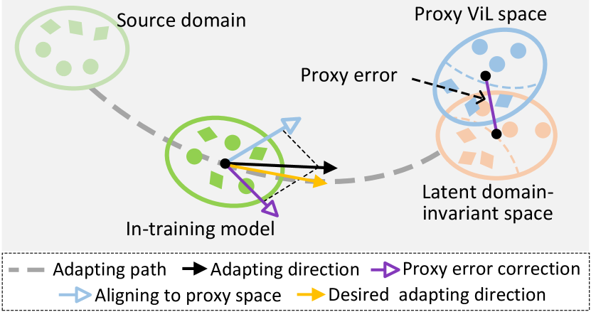
Figure 1: Conceptual illustration of ProDe.

Recently, there has been growing interest in leveraging pretrained large Vision-Language (ViL) models, e.g., CLIP [33], to help tackle transfer learning challenges. This is because ViL models have been trained with a massive amount of vision-language data, encompassing rich knowledge potentially useful for many downstream tasks. For instance, a few works [10, 18, 37] disentangle domain and category information within ViL model’s visual features by learning domain-specific using textual or visual prompts. More recently, ViL models have also been used to tackle the SFDA problem [43] for added efficacy. However, their method simply treats the ViL model’s predictions as the ground truth, which would be not valid in many unknown cases and thus making this knowledge source less effective.

To address the limitation mentioned above, in this paper, we propose a new Proxy Denoising (ProDe) approach for SFDA. In contrast to [43], we consider the ViL model/space as a noisy proxy of the latent domain-invariant space, with a need to be denoised. At the absence of any good reference models for measuring the noisy degree with the already strong ViL model’s predictions, we exploit the dynamics of domain adaptation, starting at the source model space and terminating presumably in the latent domain-invariant space, characterized by taking into account the proxy’s divergence against the domain-invariant space (Fig. 1). Specifically, we model approximately the effect of ViL model’s prediction error on domain adaption by formulating a proxy confidence theory, in relation to the discrepancy between the source domain and the current in-training model engaging in the adaptation. This results in a novel proxy denoising mechanism for ViL prediction correction. To capitalize the corrected ViL predictions more effectively, a mutual knowledge distilling regularization is further designed.

Our contributions are summarized as follows: (1) We for the first time investigate the inaccurate predictions of ViL models in the context of SFDA. (2) We formulate a novel ProDe method that reliably corrects the ViL model’s predictions under the guidance of a prediction confidence theory. A mutual knowledge distilling regularization is also introduced for capitalizing the refined proxy predictions more effectively. (3) Extensive evaluation on four standard benchmarks demonstrates that ProDe significantly outperforms previous art alternatives under the conventional closed-set settings, as well as the more challenging partial-set and open-set and generalized SFDA settings.

2 Related Work

Source-Free Domain Adaptation

The main issue with the SFDA is the lack of supervision during the model adaptation. To overcome this challenge, current methods are broadly divided into three categories. The first category involves converting SFDA to conventional UDA by introducing a pseudo-source domain. This can be achieved by building the pseudo-source domain through generative models [46, 24] or by splitting a source-distribution-like subset from the target domain [7]. The second category involves mining auxiliary information from the pre-trined source model to assist in aligning the feature distribution from the target domain to the source domain. Some of the commonly used auxiliary factors include multi-hypothesis [19], prototypes [44, 60], source distribution estimation [6], or hard samples [21]. The third category focuses on the target domain and creates additional constraints to correct the semantic noise in model transferring. In practice, domain-aware gradient control [55], data geometry such as the intrinsic neighborhood structure [39] and target data manifold [40, 41], are exploited to generate high-quality pseudo-labels [26, 5] or inject assistance in an unsupervised fashion [54]. The existing solutions refine auxiliary information from domain-specific knowledge, such as the source model and unlabeled target data, while neglecting the extensive general knowledge encoded in off-the-shelf pre-trained multimodal models.

Vision-Language Models

ViL models, such as CLIP [33] and GLIP [22], have shown promise in various tasks [25, 51] due to their ability to capture modality invariant features. There are two main lines of research related to these models. The first line aims to improve their performance. For instance, text-prompt learning [59, 10] and visual-prompt learning [50, 14] were adopted to optimize the text encoder and image encoder, respectively, using learnable prompts related to application scenarios. Some researchers have also improved the data efficiency of these models by re-purposing [1] or removing noisy data [49]. The second line of research focuses on using ViL models as external knowledge to boost downstream tasks. Related work in this area mainly follows three frameworks: Plain fusion [28], knowledge distillation [30] and information entropy regulating [3]. Taking a step further from DIFO [43] that pioneers in exploring the potential of ViL models for SFDA, we additionally consider the challenge of mitigating the noise ViL’s prediction challenge.

3 Methodology

3.1 Problem Formulation

Given two different but related domains, the labeled source and the unlabeled target domains, sharing the same $C$ categories. Let $\mathcal{X}_{s}$ and $\mathcal{Y}_{s}$ be the source samples and the corresponding labels. Similarly, the target samples and the truth target labels are denoted as $\mathcal{X}_{t}\!=\!\{{\boldsymbol{x}_{i}\}_{i=1}^{n}}$ and $\mathcal{Y}_{t}\!=\!\{{y}_{i}\}_{i=1}^{n}$, respectively, where $n$ is the sample number. With assistance of a ViL model, the SFDA task is to learn a target model $\theta_{t}\!:\!\mathcal{X}_{t}\!\to\!\mathcal{Y}_{t}$ given (1) the pre-trained source model $\theta_{s}\!:\!\mathcal{X}_{s}\!\to\!\mathcal{Y}_{s}$, (2) the unlabeled target data and (3) a ViL model providing noisy guidance. The key lies in acquiring reliable ViL predictions that we take as pseudo supervisions. This is challenging as the ViL model used is already the best in terms of knowledge comprehensiveness and domain diversity.

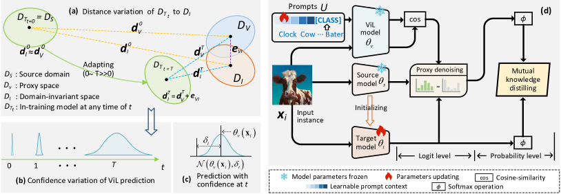
Figure 2: Left: Dynamics of effect of ViL model’s prediction error (proxy error) during proxy alignment. (a) In the initial adaptation phase, it is possible to overlook the proxy errors. However, as the in-training model approaches the proxy space, these errors become more noticeable, leading to a continuous decline in the reliability of ViL predictions as shown in (b) and (c). Right: Our ProDe capitalizes the corrected proxy, involving a mutual knowledge distilling regularization and a proxy denoising mechanism imposing adjustment on the ViL logits for more reliable ViL prediction.

To overcome this issue, we exploit the dynamics of the domain adaptation process. As shown in Fig. 2 (a), given three known spaces: Source domain $D_{S}$, far-away located latent domain-invariant space $D_{I}$, and proxy ViL space $D_{V}$ approximating $D_{I}$. The discrepancy between $D_{I}$ and $D_{V}$, leading to the ViL model’s prediction error, is referred to as proxy error $\boldsymbol{e}_{VI}$. Thus, the goal of SFDA is aligning the in-training model $D_{T_{t}}$ from $D_{S}$ to $D_{I}$ as ${\small t=0\sim T\gg 0}$. Considering $D_{I}$ is unknown, we can perform a proxy alignment to achieve this goal: Alternatively aligning to proxy $D_{V}$ whilst imposing an alignment adjusting to correct the proxy error. From this perspective, it is clear that the proxy error is the pivotal factor causing prediction noise for the proxy model. Thus, obtaining reliable ViL predictions becomes an issue of controlling the proxy error. To gain control, we establish the proxy confidence theory, whose details are elaborated in the next section.

3.2 Proxy Confidence Theory

This theory is grounded on understanding the impact of the proxy error on the domain adaptation. This can be achieved by examining the time-based motion within the proxy alignment context, which is outlined in Section 3.1.

To account for the continuity of movement, as demonstrated in Fig. 2, we consider two typical situations in the proxy alignment process, in which the distance of $D_{T_{t}}$ to $D_{V}$ and $D_{I}$ are denoted as $\boldsymbol{d}_{V}^{t}$ and $\boldsymbol{d}_{I}^{t}$, respectively.

• Case1: When $D_{T_{t}}$ is significantly far from $D_{V}$, e.g., the beginning of adaptation ($t=0$), it is hold that $\boldsymbol{d}_{I}^{0}\approx{\boldsymbol{d}}_{V}^{0}\gg\boldsymbol{e}_{VI}$. Consequently, the proxy errors can be ignored, and the ViL prediction can be deemed trustworthy.

• Case2: When $D_{T_{t}}$ approaches $D_{V}$, e.g., the later phase in the adaptation ($t\gg 0$), it becomes crucial to consider the proxy error ($\boldsymbol{d}_{I}^{t}=\boldsymbol{d}_{V}^{t}+\boldsymbol{e}_{VI}$). This is when the ViL prediction becomes less reliable.

It is seen that the proxy errors dynamically impact on this proxy alignment process, reflected in the relative relationship between $\boldsymbol{d}_{V}^{t}$ and $\boldsymbol{d}_{I}^{t}$ as:

$$\eta_{t}=\frac{\boldsymbol{d}_{I}^{t}}{\boldsymbol{d}_{V}^{t}}=\frac{\boldsymbol{d}_{V}^{t}+\boldsymbol{e}_{VI}}{\boldsymbol{d}_{V}^{t}}=\left({1+\frac{\boldsymbol{e}_{VI}}{\boldsymbol{d}_{V}^{t}}}\right),$$ (1)

where $\eta_{t}$ means the impact degree. During the proxy alignment, the ratio of ${{{\boldsymbol{e}}_{VI}}/{{\bf{d}}_{V}^{t}}}$ in Eq. (1) gradually increases from 0 (e.g., Case 1) to a non-zero value (e.g., Case 2), leading to a gradual increase in $\eta_{t}$ from 1. In other words, the impact of errors gradually increases.

Corresponding to this dynamics, as shown in Fig. 2 (b), the ViL prediction variance gradually increases, which implies a progressive decrease in the reliability of the ViL prediction. At any time $t$, we consider the ViL prediction as a Gaussian distribution $\mathcal{N}\left(\theta_{v}\left(x_{i}\right),\delta_{t}\right)$ with the mean of ViL model’s prediction $\theta_{v}\left(x_{i}\right)$ and prediction variance $\delta_{t}\propto\eta_{t}$ (Fig. 2 (c)).

Since the $\boldsymbol{e}_{VI}$ is unknown, we cannot formulate these dynamics explicitly. We consider this problem approximately: Quantifying the prediction variance with the varying confidence of the ViL model predictions. This conversion can be expressed in the form of a probability distribution with proxy confidence as:

$$\mathcal{N}\left(\theta_{v}\left(x_{i}\right),\delta_{t}\right)\Longrightarrow P\left(G_{P\left(V\right)}=True,t\right)P\left(V\right),$$ (2)

where $P(V)$ is the probability distribution of the proxy space $D_{V}$; $G_{P\left(V\right)}$ stands for a random event that the sampling results (i.e., ViL model’s prediction) from $P(V)$ is confident; $P\left(G_{P\left(V\right)}=True,t\right)$ is proxy confidence that means the probability when the event $G_{P\left(V\right)}$ is true at the time point of $t$. Within this probability context, we can formulate the proxy confidence theory for $P\left(G_{P\left(V\right)}=True,t\right)$ as detailed in Theorem 1 with proof in Appendix-A.

Theorem 1

Given a proxy alignment formulated in Section 3.1. The source domain ($D_{S}$), the domain-invariant space ($D_{I}$), the proxy space ($D_{V}$) and the in-training model ($D_{T_{t}}$) satisfy the probability distributions $P(S)$, $P(I)$, $P(V)$ and $P(T_{t})$, respectively, where $S$, $I$, $V$ and $T_{t}$ are corresponding random variables. The factor describing the credibility of $P(V)$ has a p below.

$$P\left(G_{P\left(V\right)}=True,t\right)\propto\frac{P(T_{t})}{P(S)}.$$ (3)

Given that the effect of proxy error causes the varying of the confidence factor $P\left(G_{P\left(V\right)}=True,t\right)$, as mentioned earlier, Theorem 1 provides us an insight: The effect of ViL model’s prediction error on domain adaption is approximately reflected by the discrepancy between the source domain and the current in-training model.

3.3 Capitalizing the Corrected Proxy

Overview

To capitalize the corrected proxy, we propose a novel ProDe method involving two designs: A proxy denoising mechanism and a mutual knowledge distilling regularization, as shown in Fig. 2. In this method, the proxy denoising converts the original ViL predictions to reliable ones by imposing correction on the logit level. The mutual distilling regularization encourages knowledge synchronization between the ViL model $\theta_{v}$ (teacher) and the adapting target model $\theta_{t}$ (student), coupled with a refinement for useful ingredients. In practice, this knowledge synchronization is jointly encouraged by learning target-specific prompt context (for the teacher model) and encoding the reliable proxy knowledge (for the student model). Additionally, different from previous SFDA frameworks, the source model $\theta_{s}$ in ProDe not only initiates the target model at the beginning of adapting but also supports the proxy denoising operation. ProDe’s details are presented below.

Proxy denoising

This module aims to filter out the noisy ViL prediction in an individual correction fashion, serving the target domain-specific task. Based on the results from Theorem 1 (Eq. (3)), we further convert the ViL space’s probability distribution with proxy confidence (Eq. (2)) into

$$\small\begin{split}&\log\left[P\left(G_{P\left(V\right)}=True,t\right)P\left(V\right)\right]\propto\log\left(\frac{P(T_{t})}{P(S)}P(V)\right)\\ &=\log P(V)-\left[\log P(S)-\log P(T_{t})\right].\end{split}$$ (4)

In Eq. (4), the latter two items form an adjustment to correct for the first item, essentially providing a strategy to obtain reliable ViL prediction. Inspired by Eq. (4), we design denoising mechanism as:

$$\left\{\begin{aligned} &\boldsymbol{p}^{\prime}_{i}=\phi\left(\boldsymbol{l}^{\prime}_{i}\right),~{}\boldsymbol{l}^{\prime}_{i}=\theta_{v}\left({\boldsymbol{x}}_{i},{\boldsymbol{v}}\right)-\omega\Delta_{t},\\ &\Delta_{t}=\theta_{s}\left({\boldsymbol{x}}_{i}\right)-\theta_{t}\left({\boldsymbol{x}}_{i}\right),\end{aligned}\right.$$ (5)

where $\boldsymbol{l}^{\prime}_{i}$ and $\boldsymbol{p}^{\prime}_{i}$ are the denoised ViL logit and prediction of input instance $\boldsymbol{x}_{i}$, respectively, $\boldsymbol{v}$ is the learnable prompt context and $\phi$ means softmax operation; $\Delta_{t}$ refers to the adaptive adjustment for correction, and the hyper-parameter $\omega$ specifies the correction strength.

Mutual knowledge distilling

The regularization consists of two components. First of all, given that both the ViL and target models cannot provide credible predictions, we synchronize knowledge from both sides by maximizing the unbiased mutual information between the denoised ViL prediction $\boldsymbol{p}^{\prime}_{i}$ and the target prediction $\boldsymbol{p}_{i}=\phi(\theta_{t}(\boldsymbol{x}_{i}))$. Besides, to avoid the solution collapse [11], we introduce a widely used category balance constraint [54]. Importantly, although this unsupervised design can mitigate blindly trusting either model, the synchronized knowledge is not fully useful, being misled by the noisy interaction. Therefore, we additionally refine the useful parts by introducing a classification sub-task with the supervision of pseudo hard labels.

Formally, we can summarize the designs mentioned above to the following objective.

$${L}_{ProDe}= \min_{\theta_{t},\boldsymbol{v}}\alpha\overbrace{\left(-\mathbb{E}_{{\boldsymbol{x}}_{i}\in{\mathcal{X}_{t}}}{\boldsymbol{\rm{MI}}}\left(\boldsymbol{p}^{\prime}_{i},\boldsymbol{p}_{i}\right)+\gamma{\sum_{c=1}^{C}{\bar{q}}_{c}\log{\bar{q}}_{c}}\right)}^{{L}_{Syn}}$$ (6)

$$-\beta\overbrace{\mathbb{E}_{{\boldsymbol{x}}_{i}\in{\mathcal{X}_{t}}}\sum_{c=1}^{C}\mathbbm{{1}}{\left[c=y^{\prime}_{i}\right]}\log{p}_{i,c}}^{L_{Ref}},$$

where ${\boldsymbol{\rm{MI}}}(\cdot,\cdot)$ computes the mutual information [13]; the second item is the balance loss, $C$ is the category number, $\bar{q}_{c}=\frac{1}{n}\sum_{i=1}^{n}{q}_{i,c}$ is $c$-th element of $\bar{\boldsymbol{q}}$, in which $\bar{\boldsymbol{q}}$ is are empirical label distribution over the $C$ categories, ${q}_{i,c}$ is the probability value of target prediction $\theta_{t}\left({\boldsymbol{x}}_{i}\right)$ in the $c$-th category; ${p}_{i,c}$ is the $c$-th element of $\boldsymbol{p}_{i}$, $\mathbbm{{1}}{\left[c=y^{\prime}_{i}\right]}$ is a one-hot encoding of hard category label $y^{\prime}_{i}$ predicted by $\boldsymbol{p}^{\prime}_{i}$. With regulating of Eq. (6), we perform the model training iteration-wise. The concrete procedure is summarized in the algorithm provided in Alg. 1.

Algorithm 1 Training of ProDe

Input: Source model $\theta_{s}$, ViL model $\theta_{v}$, target dataset $\mathcal{X}_{t}$, $C$ prompts with context $\boldsymbol{v}$, #iteration $M$.
Procedure:

1:  Initialisation: Set target model $\theta_{t}=\theta_{s}$, prompt context $\boldsymbol{v}=$”a photo of a”.

2:  for $m$ = 1:$M$ do

3:     Sample a batch $\mathcal{X}_{t}^{b}$ from $\mathcal{X}_{t}$.

4:     Forward updated prompts and $\mathcal{X}_{t}^{b}$ through $\theta_{v}$.

5:     Forward $\mathcal{X}_{t}^{b}$ through $\theta_{t}$.

6:     Conduct proxy denoising for the ViL predictions of $\mathcal{X}_{t}^{b}$ (Eq. (5)).

7:     Update model $\theta_{t}$ and prompt context $\boldsymbol{v}$ by optimizing objective ${L}_{{ProDe}}$ (Eq. (6)).

8:  end for

9:  return Adapted target model $\theta_{t}$.

4 Experiments

Datasets

In this paper, the ProDe method is evaluated on four widely used benchmarks for domain adaptation problems as follows. Office-31 [35] is a small-scaled dataset including three domains, i.e., Amazon (A), Webcam (W), and Dslr (D), all of which are taken of real-world objects in various office environments. The dataset has 4,652 images of 31 categories in total. Office-Home [47] is a medium-scale dataset that is mainly used for domain adaptation, all of which contains 15k images belonging to 65 categories from working or family environments. The dataset has four distinct domains, i.e., Artistic images (Ar), Clip Art (Cl), Product images (Pr), and Real-word images (Rw). VisDA [31] is a large-scale dataset with 12 types of synthetic to real transfer recognition tasks. The source domain contains 152k synthetic images (Sy), whilst the target domain has 55k real object images (Re) from the famous Microsoft COCO dataset. DomainNet-126 [36] is another challenging large-scale dataset. It has been created by removing severe noisy labels from the original DomainNet dataset [32] containing 600k images of 345 classes from 6 domains of varying image styles. The dataset is further divided into four domains: Clipart (C), Painting (P), Real (R), and Sketch (S), and contains 145k images from 126 classes.

SFDA settings We consider three distinct SFDA settings: conventional closed-set, partial-set, open-set (the details are initialized in SHOT [26]) and generalized SFDA settings (the details are initialized in GDA [55]). The experiment implementation details are provided in Appendix B.

4.1 Competitors

To evaluate ProDe, we select 22 related comparisons divided into three groups. (1) The first one includes the source model results (termed Source) and CLIP zero-shot (termed CLIP) [33]. (2) The second one includes five state-of-the-art UDA methods based on multimodality: DAPL-R [10], PADCLIP-R [18], ADCLIP-R [37] PDA-R [2], DAMP-R [8]. All of them introduce CLIP to solve the UDA problem. The suffix of “-R” means that the image-encoder in CLIP uses the backbone of ResNet. (3) The third one comprises 13 current state-of-the-art SFDA models: SHOT [26], NRC [54], GKD [38], HCL [12], AaD [56], AdaCon [4], CoWA [20], ELR [57], PLUE [27], CRS [58], CPD [60], TPDS [41], and DIFO [43]. Among them, DIFO is the multimodal SFDA method. (4) The fourth one are two state-of-the-art generalized SFDA methods GDA [55] and PSAT-ViT [42].

To provide a comprehensive comparison, we have initiated ProDe into a strong version ProDe-V and a weak version ProDe-R. The main difference between these two versions is the use of different backbones for the CLIP image-encoder. Specifically, ProDe-V employs the backbone of ViT-B/32 across all datasets, whilst ProDe-R uses ResNet101 on the VisDA dataset and ResNet50 on the other three datasets. As for the previous best multimodal method, DIFO [43], we also give the same version, termed DIFO-R and DIFO-V, for a fair comparison.

Table 1: Closed-set SFDA results (%) on the Office-31 dataset.

Method	Venue	SF	M	A$\to$D	A$\to$W	D$\to$A	D$\to$W	W$\to$A	W$\to$D	Avg.
Source	–	✗	✗	79.1	76.6	59.9	95.5	61.4	98.8	78.6
SHOT [26]	ICML20	✗	✗	93.7	91.1	74.2	98.2	74.6	100.	88.6
NRC [54]	NIPS21	✗	✗	96.0	90.8	75.3	99.0	75.0	100.	89.4
GKD [38]	IROS21	✗	✗	94.6	91.6	75.1	98.7	75.1	100.	89.2
HCL [12]	NIPS21	✗	✗	94.7	92.5	75.9	98.2	77.7	100.	89.8
AaD [56]	NIPS22	✗	✗	96.4	92.1	75.0	99.1	76.5	100.	89.9
AdaCon [4]	CVPR22	✗	✗	87.7	83.1	73.7	91.3	77.6	72.8	81.0
CoWA [20]	ICML22	✗	✗	94.4	95.2	76.2	98.5	77.6	99.8	90.3
ELR [57]	ICLR23	✗	✗	93.8	93.3	76.2	98.0	76.9	100.	89.6
PLUE [27]	CVPR23	✗	✗	89.2	88.4	72.8	97.1	69.6	97.9	85.8
CPD [60]	PR24	✗	✗	96.6	94.2	77.3	98.2	78.3	100.	90.8
TPDS [41]	IJCV24	✗	✗	97.1	94.5	75.7	98.7	75.5	99.8	90.2
DIFO-R [43]	CVPR24	✓	✓	93.6	92.1	78.5	95.7	78.8	97.0	89.3
DIFO-V [43]	CVPR24	✓	✓	97.2	95.5	83.0	97.2	83.2	98.8	92.5
ProDe-R	–	✓	✓	92.6	93.2	80.9	94.6	81.0	98.0	90.0
ProDe-V	–	✓	✓	96.6	96.4	83.1	96.9	82.9	99.8	92.6

Table 2: Closed-set SFDA results (%) on the Office-Home and VisDA dataset. SF and M means source-free and multimodal, respectively. The full results on VisDA are provided in Appendix C.1.

Method	Venue	SF	M	Office-Home													VisDA
				Ar$\to$Cl	Ar$\to$Pr	Ar$\to$Rw	Cl$\to$Ar	Cl$\to$Pr	Cl$\to$Rw	Pr$\to$Ar	Pr$\to$Cl	Pr$\to$Rw	Rw$\to$Ar	Rw$\to$Cl	Rw$\to$Pr	Avg.	Sy$\to$Re
Source	–	–	-	43.7	67.0	73.9	49.9	60.1	62.5	51.7	40.9	72.6	64.2	46.3	78.1	59.2	49.2
DAPL-R [10]	TNNLS23	✗	✓	54.1	84.3	84.8	74.4	83.7	85.0	74.5	54.6	84.8	75.2	54.7	83.8	74.5	86.9
PADCLIP-R [18]	ICCV23	✗	✓	57.5	84.0	83.8	77.8	85.5	84.7	76.3	59.2	85.4	78.1	60.2	86.7	76.6	88.5
ADCLIP-R [37]	ICCVW23	✗	✓	55.4	85.2	85.6	76.1	85.8	86.2	76.7	56.1	85.4	76.8	56.1	85.5	75.9	87.7
PDA-R [2]	AAAI24	✗	✓	55.4	85.1	85.8	75.2	85.2	85.2	74.2	55.2	85.8	74.7	55.8	86.3	75.3	86.4
DAMP-R [8]	CVPR24	✗	✓	59.7	88.5	86.8	76.6	88.9	87.0	76.3	59.6	87.1	77.0	61.0	89.9	78.2	88.4
SHOT [26]	ICML20	✓	✗	56.7	77.9	80.6	68.0	78.0	79.4	67.9	54.5	82.3	74.2	58.6	84.5	71.9	82.7
NRC [54]	NIPS21	✓	✗	57.7	80.3	82.0	68.1	79.8	78.6	65.3	56.4	83.0	71.0	58.6	85.6	72.2	85.9
GKD [38]	IROS21	✓	✗	56.5	78.2	81.8	68.7	78.9	79.1	67.6	54.8	82.6	74.4	58.5	84.8	72.2	83.0
AaD [56]	NIPS22	✓	✗	59.3	79.3	82.1	68.9	79.8	79.5	67.2	57.4	83.1	72.1	58.5	85.4	72.7	88.0
AdaCon [4]	CVPR22	✓	✗	47.2	75.1	75.5	60.7	73.3	73.2	60.2	45.2	76.6	65.6	48.3	79.1	65.0	86.8
CoWA [20]	ICML22	✓	✗	56.9	78.4	81.0	69.1	80.0	79.9	67.7	57.2	82.4	72.8	60.5	84.5	72.5	86.9
ELR [57]	ICLR23	✓	✗	58.4	78.7	81.5	69.2	79.5	79.3	66.3	58.0	82.6	73.4	59.8	85.1	72.6	85.8
PLUE [27]	CVPR23	✓	✗	49.1	73.5	78.2	62.9	73.5	74.5	62.2	48.3	78.6	68.6	51.8	81.5	66.9	88.3
CPD [60]	PR24	✓	✗	59.1	79.0	82.4	68.5	79.7	79.5	67.9	57.9	82.8	73.8	61.2	84.6	73.0	85.8
TPDS [41]	IJCV24	✓	✗	59.3	80.3	82.1	70.6	79.4	80.9	69.8	56.8	82.1	74.5	61.2	85.3	73.5	87.6
DIFO-R [43]	CVPR24	✓	✓	62.6	87.5	87.1	79.5	87.9	87.4	78.3	63.4	88.1	80.0	63.3	87.7	79.4	88.8
DIFO-V [43]	CVPR24	✓	✓	70.6	90.6	88.8	82.5	90.6	88.8	80.9	70.1	88.9	83.4	70.5	91.2	83.1	90.3
ProDe-R	–	✓	✓	66.0	91.2	90.8	81.4	91.4	90.5	82.2	67.3	90.8	83.6	67.7	91.6	82.9	89.9
ProDe-V	–	✓	✓	74.6	92.9	92.4	84.4	93.0	92.2	83.8	74.8	92.4	84.9	75.2	93.7	86.2	91.6

Table 3: Closed-set SFDA results (%) on the DomainNet-126 dataset. SF and M means source-free and multimodal, respectively.

Method	Venue	SF	M	C$\to$P	C$\to$R	C$\to$S	P$\to$C	P$\to$R	P$\to$S	R$\to$C	R$\to$P	R$\to$S	S$\to$C	S$\to$P	S$\to$R	Avg.
Source	–	–	–	44.6	59.8	47.5	53.3	75.3	46.2	55.3	62.7	46.4	55.1	50.7	59.5	54.7
DAPL-R [10]	TNNLS23	✗	✓	72.4	87.6	65.9	72.7	87.6	65.6	73.2	72.4	66.2	73.8	72.9	87.8	74.8
ADCLIP-R [37]	ICCVW23	✗	✓	71.7	88.1	66.0	73.2	86.9	65.2	73.6	73.0	68.4	72.3	74.2	89.3	75.2
DAMP-R [8]	CVPR24	✗	✓	76.7	88.5	71.7	74.2	88.7	70.8	74.4	75.7	70.5	74.9	76.1	88.2	77.5
SHOT [26]	ICML20	✓	✗	63.5	78.2	59.5	67.9	81.3	61.7	67.7	67.6	57.8	70.2	64.0	78.0	68.1
GKD [38]	IROS21	✓	✗	61.4	77.4	60.3	69.6	81.4	63.2	68.3	68.4	59.5	71.5	65.2	77.6	68.7
NRC [54]	NIPS21	✓	✗	62.6	77.1	58.3	62.9	81.3	60.7	64.7	69.4	58.7	69.4	65.8	78.7	67.5
AdaCon [4]	CVPR22	✓	✗	60.8	74.8	55.9	62.2	78.3	58.2	63.1	68.1	55.6	67.1	66.0	75.4	65.4
CoWA [20]	ICML22	✓	✗	64.6	80.6	60.6	66.2	79.8	60.8	69.0	67.2	60.0	69.0	65.8	79.9	68.6
PLUE [27]	CVPR23	✓	✗	59.8	74.0	56.0	61.6	78.5	57.9	61.6	65.9	53.8	67.5	64.3	76.0	64.7
TPDS [41]	IJCV24	✓	✗	62.9	77.1	59.8	65.6	79.0	61.5	66.4	67.0	58.2	68.6	64.3	75.3	67.1
DIFO-R [43]	CVPR24	✓	✓	73.8	89.0	69.4	74.0	88.7	70.1	74.8	74.6	69.6	74.7	74.3	88.0	76.7
DIFO-V [43]	CVPR24	✓	✓	76.6	87.2	74.9	80.0	87.4	75.6	80.8	77.3	75.5	80.5	76.7	87.3	80.0
ProDe-R	–	✓	✓	79.3	91.0	75.3	80.0	90.9	75.6	80.4	78.9	75.4	80.4	79.2	91.0	81.5
ProDe-V	–	✓	✓	83.2	92.4	79.0	85.0	92.3	79.3	85.5	83.1	79.1	85.5	83.4	92.4	85.0

4.2 Comparison Results

Comparisons on closed-set SFDA setting. Tab. 1$\sim$3 lists the quantitative comparisons on the four evaluation datasets. Both ProDe-R and ProDe-V beat all non-multimodal SFDA methods with a large margin. Compared with the second-best method CPD (on Office-31), TPDS (on Office-Home), PLUE (on VisDA) and GKD (on DomainNet-126), ProDe-V improves by 1.8%, 12.7% 3.3% and 16.3% in average accuracy respectively. As for those multimodal methods, including both UDA and SFDA, ProDe also beat them in the same backbone setting. Specifically, as using ResNet, ProDe-R surpasses the second-best UDA method DAMP-R (on Office-Home), PADCLIP-R (on VisDA) and DAMP-R (on DomainNet-126) by 4.7%, 1.4% and 4.0% in average accuracy respectively. In particular, compared with the multimodal SFDA method DIFO, ProDe improves by 4.8% and 5.0% (on DomainNet-126) at most using ResNet and ViT-B/32, respectively. Actually, the weak version of our method, ProDe-R, is competitive with the strong version of DIFO, DIFO-V. All of these results indicate that ProDe can significantly boost the cross-domain adaptation under the closed-set SFDA setting.

Comparison to CLIP prediction results. It only makes sense for ProDe to outperform CLIP. To assess this, we conducted a quantitative comparison between our model’s adaptation performance and CLIP’s zero-shot performance. The results of our model are reported with average accuracy. As reported in Tab. 4, ProDe-R and ProDe-V improve at least by 6.2 % (on VisDA) and 8.7% (on VisDA and DomainNet-126), respectively, compared with CLIP’s results on the four datasets. This result shows that the multimodal CLIP space only approximates the domain invariant space, highlighting the necessity of pursuing reliable ViL prediction, which this paper focuses on.

Comparison on partial-set and open-set settings. For a complete evaluation, we also evaluate ProDe on two variation scenarios: partial-set and open-set settings. As reported in Tab. 5, ProDe-V achieves a gain of 0.6% (partial-set) and 6.7% (open-set) compared with the best competitor DIFO-V.

Comparison on generalized SFDA settings. The generalized SFDA is an extended problem of closed-set SFDA, highlighting the anti-forgetting ability on the seen source domain. The same as [55], we adopt the harmonic mean accuracy as evaluation protocol, which is computed by ${H}=({2*Acc_{s}*Acc_{t}})/({Acc_{s}+Acc_{t}})$ where $Acc_{s}$ and $Acc_{t}$ are the accuracies of the adapted target model on the source domain and the target domain, respectively. Note that the $Acc_{s}$ is computed based on the source-testing set. The same to [55, 42], on the source domain, the ratio of training and testing sets is 9:1. To evaluate effectiveness, two generalized SFDA methods, GDA and PSAT-ViT, are chosen as additional comparisons. Based on Tab. 6, it is seen that ProDe-V outperforms all comparisons in terms of H-accuracy, even those designed to imitate forgetting. Meanwhile, both ProDe-R and ProDe-V deliver balanced results across the source and target domains. This is due to the correction in the proxy denoising, which incorporates information from the source model, thereby mitigating forgetting of the source domain.

4.3 Model Analysis

Feature distribution visualization. Based on the task Cl$\to$Ar in Office-Home, we conducted a toy experiment to visualize the feature distribution of ProDe using the t-SNE tool. Meanwhile, five comparisons are considered, including CLIP-V, SHOT, TPDS, DIFO-V and Oracle. Among them, CLIP-V is the zero-shot result, and Oracle is trained on domain Cl with the real labels. For a clear view, all results are presented in 3D density charts. As shown in Fig. 3, from CLIP-V to Oracle, category clustering becomes increasingly apparent. The distribution shape of DIFO-V and ProDe-V is closer to the expert model than that of non-multimodal methods, SHOT and TPDS. Furthermore, although DIFO-V and ProDe-V have a similar pattern, ProDe-V’s shape is more detailed with Oracle.

Table 4: Comparison to CLIP in average accuracy (%). The full results are provided in Appendix C.1.

Method	Office-31	Office-Home	VisDA	DomainNet-126
CLIP-R [33]	71.4	72.1	83.7	72.7
ProDe-R	90.0	82.9	89.9	81.5
CLIP-V [33]	79.8	76.1	82.9	76.3
ProDe-V	92.6	86.2	91.6	85.0

Table 5: Partial-set and open-set results (%) on Office-Home. The full results are provided in Appendix C.1.

Partial-set SFDA	Venue	Avg.	Open-set SFDA	Venue	Avg.
Source	–	62.8	Source	–	46.6
SHOT [26]	ICML20	79.3	SHOT [26]	ICML20	72.8
HCL [12]	NIPS21	79.6	HCL [12]	NIPS21	72.6
CoWA [20]	ICML22	83.2	CoWA [20]	ICML22	73.2
AaD [56]	NIPS22	79.7	AaD [56]	NIPS22	71.8
CRS [58]	CVPR23	80.6	CRS [58]	CVPR23	73.2
DIFO-V [43]	CVPR24	85.6	DIFO-V [43]	CVPR24	75.9
ProDe-V	–	86.2	ProDe-V	–	82.6

Table 6: Generalized SFDA results (%) on Office-Home. S, T are the results of the adapted target model on the source and target domains, i.e., $Acc_{s}$, $Acc_{t}$, respectively; WAD means With Anti-forgetting Design. Appendix C.1 gives the full results.

Method	Venue	WAD	Avg.
			S (98.1-S)	T	H
Source	–	✗	98.1	59.2	73.1
SHOT [26]	ICML20	✗	84.2 (13.9)	71.8	77.5
GKD [38]	IROS21	✗	86.8 (11.3)	72.5	79.0
NRC [54]	NIPS21	✗	91.3 (6.8)	72.3	80.7
AdaCon [4]	CVPR22	✗	88.2 (9.9)	65.0	74.8
CoWA [20]	ICML22	✗	91.8 (6.3)	72.4	81.0
PLUE [27]	CVPR23	✗	96.3 (1.8)	66.9	79.0
TPDS [41]	IJCV24	✗	83.8 (14.3)	73.5	78.3
GDA [55]	ICCV21	✓	80.0 (18.1)	70.2	74.4
PSAT-ViT [42]	TMM24	✓	86.4 (11.7)	83.6	85.0
DIFO-R [43]	CVPR24	✗	78.3 (19.8)	79.4	78.8
DIFO-V [43]	CVPR24	✗	78.0 (20.1)	83.1	80.5
ProDe-R	–	✗	83.3 (14.8)	82.9	83.1
ProDe-V	–	✗	84.1 (14.0)	86.2	85.1

Ablation studies. This part of the experiment isolates the effect of the objective components in Eq. (6) and proxy denoising. Tab. 7 presents the ablation study results, with the baseline being the results of the source model (1 row). When $\mathcal{L}_{Syn}$ or $\mathcal{L}_{Ref}$ is used alone (2, 3 row), their performances show similar average accuracy. However, when they work together, the best results are achieved (4 row). This comparison indicates that the proposed two losses jointly contribute to the final performance.

Furthermore, removing proxy denoising (5 row) from the model leads to a decrease in average accuracy by 2.0%, which confirms its effectiveness. To evaluate the effect of components in the proxy denoising design, we respectively remove the source and target models’ logits (see Eq. (5)) to obtain two ProDe variation methods, ProDe-V w/o source and ProDe-V w/o target. As listed in Tab. 7 (6, 7 row), using either adjustment alone led to a significant decrease in performance, confirming the effectiveness of our difference-based correction strategy. Also, we perform the correction at the probability level, instead of the logit level, in another comparison ProDe-V w prob. The 3.0% decrease (compared with ProDe) confirms the rationality of correction on logits.

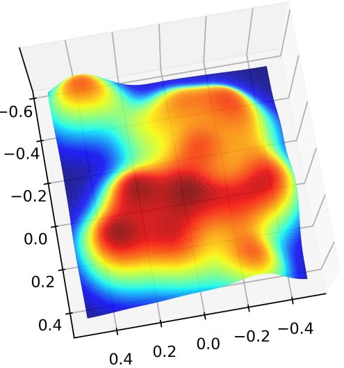
(a)

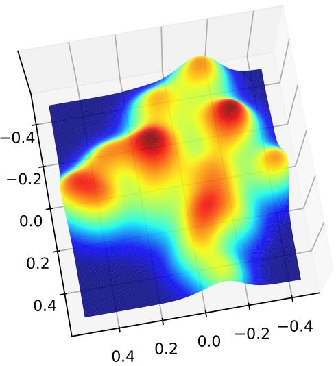
(b)

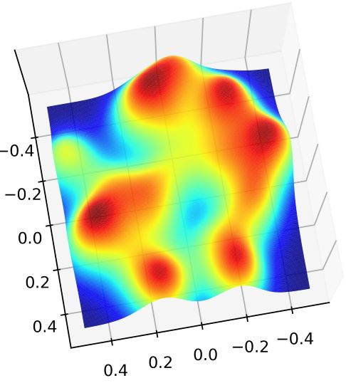
(c)

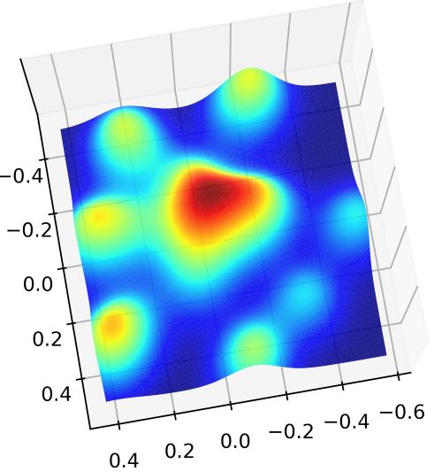
(d)

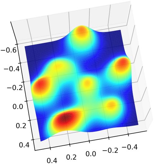
(e)

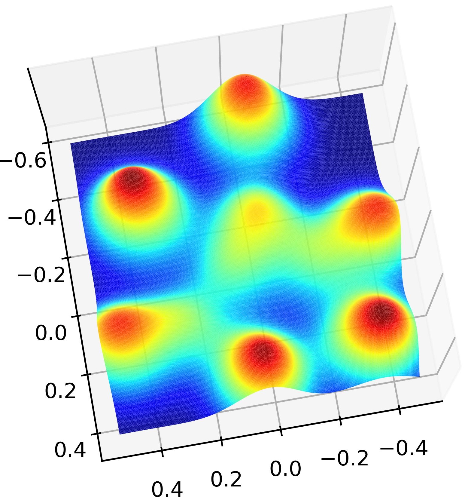
(f)

Figure 3: Feature visualization comparison in 3D density charts.

Table 7: Ablation study results (%).

#	$L_{\rm{Syn}}$	$L_{\rm{Ref}}$	Office-31	Office-Home	VisDA	Avg.
1	✗	✗	78.6	59.2	49.2	62.3
2	✓	✗	91.8	78.8	90.2	86.9
3	✗	✓	86.5	83.2	90.7	86.8
4	✓	✓	92.6	86.2	91.6	90.1
5	ProDe-V w/o pd		90.5	83.9	89.9	88.1
6	ProDe-V w/o source		91.2	84.6	90.2	88.7
7	ProDe-V w/o target		80.1	83.5	90.8	84.8
8	ProDe-V w proba		86.8	83.3	91.3	87.1

4.4 Quantitative Analysis of Proxy Denoising in Proxy Alignment View

In this part, we make a feature space shift analysis using the measure of MMD (maximum mean discrepancy) distance to verify whether our ProDe method ensures the proxy alignment. In this experiment, we initially train a domain-invariant Oracle model over all Office-Home data with real labels, and use the logits to express the domain-invariant space $O$. Sequentially, we perform a transfer experiment of Ar$\to$Cl. During this adaptation, there are $K$ (epoch number) intermediate adapting target models. We feedforward the target data through each intermediate model and take the logits as a space. Thus, we obtain $K$ intermediate target feature spaces $\{U_{k}\}_{k=1}^{K}$. These intermediate spaces can lead to three different kinds of distances corresponding to these frozen spaces, termed $\boldsymbol{d}_{S}^{t}$ (to the source domain), $\boldsymbol{d}_{O}^{t}$ (to the Oracle space) and $\boldsymbol{d}_{V}^{t}$ (to the proxy CLIP space). In practice, the CLIP image encoder’s backbone is set to ViT-B/32.

Fig. 4 (a) displays the varying curves (epoch view) of $\boldsymbol{d}_{S}^{t}$, $\boldsymbol{d}_{O}^{t}$ and $\boldsymbol{d}_{V}^{t}$. As expected, $\boldsymbol{d}_{S}^{t}$ increases, along with a decreasing on $\boldsymbol{d}_{O}^{t}$. Meanwhile, $\boldsymbol{d}_{V}^{t}$ exhibits a V-shaped trend. For a clear view, we zoom into the first epoch and observe its variation details, as shown in Figure 4 (b). In particular, there is a smooth transition from decrease to increase on the curve of $\boldsymbol{d}_{V}^{t}$. This phenomenon indicates that the in-training model indeed approaches the proxy space and then moves away from it to close the domain-invariant space as our proxy error control gradually comes into play.

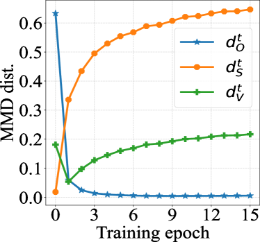
(a)

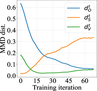
(b)

(c)

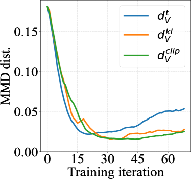
(d)

Figure 4: Analysis for proxy denoising on the Al$\to$Cl task in Office-Home. (a) The MMD-distance varying curves (epoch view) between the intermediate spaces to the source, oracle and proxy CLIP spaces, respectively, i.e., $\boldsymbol{d}_{S}^{t}$, $\boldsymbol{d}_{O}^{t}$ and $\boldsymbol{d}_{V}^{t}$. (b) The details of $\boldsymbol{d}_{V}^{t}$ (iteration view) during the first epoch. (c) The accuracy curves of typical signals during the adaptation. (d) The MMD-distance varying curves of ProDe ($\boldsymbol{d}_{V}^{t}$), ProDe-KL ($\boldsymbol{d}_{V}^{kl}$), ProDe-CLIP ($\boldsymbol{d}_{V}^{clip}$) during the first epoch (iteration view).

Correspondingly, we also provide the accuracy varying curves of two typical signals in Fig. 4 (c), including the target prediction (termed ProDe) and the denoised CLIP prediction (termed PRO). In this experiment, CLIP zero-shot result (termed CLIP) is the baseline. It is seen that PRO is better than ProDe in the early phase (0$\sim$7 epoch) and surpassed by ProDe in the rest epochs. The results indicate that the guidance of reliable ViL predictions can boost the adaptation performance. Meanwhile, the PRO and ProDe curves closely resemble each other. It is understandable that the current prediction of the adapting target model, $\theta_{t}(\boldsymbol{x}_{i})$, is utilized to adjust the raw ViL prediction (see Eq. (5)).

To better understand the impact of proxy denoising, we also conduct a comparison experiment using two variations of ProDe. In ProDe-KL, the loss $L_{Syn}$ is changed to conventional KL-Divergence, whilst in ProDe-CLIP, the training is based on the raw ViL prediction with proxy denoising. Employing the same MMD-distance quantification method mentioned above, we can plot two distance curves to the proxy space, termed $\boldsymbol{d}_{V}^{kl}$, $\boldsymbol{d}_{V}^{clip}$. In Fig. 4 (d), it is evident that ProDe moves away from the proxy space more quickly than the other two comparisons. This result suggests that ProDe is more responsive to proxy errors, resulting in agile error correction to match desired adapting direction.

5 Conclusion

The success of multimodal foundation models has sparked interest in transferring general multimodal knowledge to assist with domain-specific tasks, particularly in the field of transfer learning. However, for label-free scene scenarios such as SFDA discussed in this paper, the issue of filtering out noise from multimodal foundation models has been largely overlooked. To address this fundamental issue, this paper introduces a new ProDe approach. We fist introduce a new approach called proxy denoising, which corrects the raw ViL predictions and provides reliable ViL guidance. This approach is based on a novel proxy confidence theory that we developed by modeling the impact of the proxy error between the proxy ViL space and the latent domain-invariant space, using the adaptation dynamics in the proxy alignment. Additionally, we propose a mutual distilling method to make use of the reliable proxy. Extensive experiment results indicate that our ProDe can achieve state-of-the-art results with significant improvements on four challenging datasets, confirming its effectiveness.

Appendix A Proof of Theorem 1

Restatement of Theorem 1

Given a proxy alignment formulated in section 3.1. The source domain ($D_{S}$), the domain-invariant space ($D_{I}$), the proxy space ($D_{V}$) and the in-training model ($D_{T_{t}}$) satisfy the probability distributions $P(S)$, $P(I)$, $P(V)$ and $P(T_{t})$, respectively, where $S$, $I$, $V$ and $T_{t}$ are corresponding random variables. The factor describing the credibility of $P(V)$ has a relation below.

$$P\left(G_{P\left(V\right)}=True,t\right)\propto\frac{P(T_{t})}{P(S)}.$$

Proof 1

We use the spatial distance relation to represent the variation in confidence of ViL prediction, which is causally linked to the variation in distance to $D_{I}$, as demonstrated in Fig. 2 (a). At any given time $t$, the correction factor can be expressed as

$$\begin{split}P\left(G_{P\left(V\right)}=True,t\right)\propto\frac{Distance(D_{T_{t}},D_{I})}{Distance(D_{S},D_{I})}=\frac{\boldsymbol{d}_{I}^{t}}{\boldsymbol{d}_{S}},\end{split}$$ (7)

where $\boldsymbol{d}_{I}^{t}$ and $\boldsymbol{d}_{S}$ refers to the distance from $D_{T_{t}}$ and $D_{S}$ to $D_{I}$, respectively. Easily finding, Eq. (7) satisfies the reliability feature of gradually decreasing from 1 to 0 as $D_{T_{t}}$ evolves from $D_{S}$ to $D_{I}$.

To account for the fact that spaces are defined by probability distributions, we instantiate the space distance using the widely used measurement of KL-divergence. This gives us:

$$\small\begin{split}\frac{\boldsymbol{d}_{I}^{t}}{\boldsymbol{d}_{S}}&=\frac{KL\left(P(T_{t})||P(I)\right)}{KL\left(P(S)||P(I)\right)}=\frac{\int_{T_{t}}P(T_{t})\log\frac{P(T_{t})}{P(I)}dT_{t}}{\int_{S}P(S)\log\frac{P(S)}{P(I)}dS}\\ &=\frac{-\int_{T_{t}}P(T_{t})\log P(T_{t})dT_{t}+\int_{T_{t}}P(T_{t})\log P(I)dT_{t}}{-\int_{S}P(S)\log P(S)dS+\int_{S}P(S)\log P(I)dS}\\ &=\frac{H(T_{t})+\log P(I)}{H(S)+\log P(I)}\\ &=\frac{H(T_{t})}{H(S)},\end{split}$$ (8)

where $H(\cdot)$ stands for the information entropy. Since $D_{I}$ is an domain-invariant space, $P(I)$ always outputs 1 for the category of interesting, such that $\log P(I)=0$. Eq. (7) can be further converted to

$$\small\begin{split}\frac{H(T_{t})+\log P(I)}{H(S)+\log P(I)}=\frac{H(T_{t})}{H(S)}\propto\frac{P(T_{t})}{P(S)}\end{split}$$ (9)

Appendix B Implementation Details

Souce model pre-training. For all transfer tasks on the three datasets, we train the source model $\theta_{s}$ on the source domain in a supervised manner using the following objective of the classic cross-entropy loss with smooth label, totally the same as other methods [26, 54, 40].

$$\begin{split}L_{\rm{s}}\left(\mathcal{X}_{s},\mathcal{Y}_{s};\theta_{s}\right)=-\mathbb{E}_{{\boldsymbol{x}}_{i}^{s}\in{\mathcal{X}_{s}}}\sum_{c=1}^{C}\tilde{\mathbbm{1}}\left[c=y_{i}^{s}\right]\log{p}_{i,c}^{s},\end{split}$$

where ${p}_{i,c}^{s}$ is the $c$-th element of $\boldsymbol{p}_{i}^{s}=\phi(\theta_{s}({\boldsymbol{x}}_{i}^{s}))$ that is the category probability vector of input instance ${\boldsymbol{x}}_{i}^{s}$ after $\theta_{s}$ conversion with ending softmax operation $\phi$; $\tilde{\mathbbm{1}}\left[c=y_{i}^{s}\right]=(1-\sigma){\kern 2.0pt}{\mathbbm{1}}\left[c=y_{i}^{s}\right]+\sigma/C$ is the smooth label [29], in which ${\mathbbm{1}}\left[c=y_{i}^{s}\right]$ is a one-hot encoding of hard label $y_{i}^{s}$ and $\sigma=0.1$. The source dataset is divided into the training set and testing set in a 0.9:0.1 ratio.

Network setting. The ProDe framework involves two networks, namely the target model and the ViL model. In practice, the target model comprises a deep architecture-based feature extractor and a classifier that consists of a fully connected layer and a weight normalization layer. As seen in previous work [53, 26, 34], the deep architecture is transferred from the deep models pre-trained on ImageNet. Specifically, ResNet-50 is used on Office-31 and Office-Home, whilst ResNet-101 is employed on VisDA and Domain-Net. As for the ViL model, we choose CLIP to instantiate it where the text encoder adopts Transformer structure and the image encoder takes ResNet or ViT-B/32 according to the specific implementation of ProDe, including ProDe-R and ProDe-V. To be specific, ProDe-V uses the ViT-B/32 architecture suggested in CLIP as the image encoder, while ProDe-RES uses ResNet as the backbone. More specifically, the same ResNet-101 is used for VisDA, and ResNet-50 is used for the remaining datasets, just like the target model mentioned earlier.

In this paper, we use two versions of the image encoder for the implementation of ProDe. These are ProDe-R and ProDe-V. To be specific, ProDe-V uses the ViT-B/32 architecture suggested in CLIP as the image encoder, while ProDe-R uses ResNet as the backbone. The same ResNet-101 is used for VisDA, and ResNet-50 is used for the remaining datasets, just like the target model mentioned earlier.

Hyper-parameter setting. Our ProDe model contains the correction strength factor $\omega$ in Eq. (5) and two trade-off parameters $\alpha$, $\beta$ and $\gamma$ in objective $L_{\rm{ProDe}}$ (Eq. (6)). On all four datasets, we set $(\omega,\alpha,\beta)=(1,1,0.4)$. The setting of $\gamma=1.0/1.0/0.1/0.5$ is employed on Office-31, Office-Home, VisDA, DomainNet-126, respectively.

Table 8: Full results (%) of closed-set SFDA on the VisDA dataset. SF and M mean source-free and multimodal, respectively.

Method	Venue	SF	M	plane	bcycl	bus	car	horse	knife	mcycl	person	plant	sktbrd	train	truck	Perclass
Source	-	-	-	60.7	21.7	50.8	68.5	71.8	5.4	86.4	20.2	67.1	43.3	83.3	10.6	49.2
DAPL-R [10]	TNNLS23	✗	✓	97.8	83.1	88.8	77.9	97.4	91.5	94.2	79.7	88.6	89.3	92.5	62.0	86.9
PADCLIP-R [18]	ICCV23	✗	✓	96.7	88.8	87.0	82.8	97.1	93.0	91.3	83.0	95.5	91.8	91.5	63.0	88.5
ADCLIP-R [37]	ICCVW23	✗	✓	98.1	83.6	91.2	76.6	98.1	93.4	96.0	81.4	86.4	91.5	92.1	64.2	87.7
PDA-R [2]	AAAI24	✗	✓	97.2	82.3	89.4	76.0	97.4	87.5	95.8	79.6	87.2	89.0	93.3	62.1	86.4
DAMP-R [8]	CVPR24	✗	✓	97.3	91.6	89.1	76.4	97.5	94.0	92.3	84.5	91.2	88.1	91.2	67.0	88.4
SHOT [26]	ICML20	✓	✗	95.0	87.4	80.9	57.6	93.9	94.1	79.4	80.4	90.9	89.8	85.8	57.5	82.7
NRC [54]	NIPS21	✓	✗	96.8	91.3	82.4	62.4	96.2	95.9	86.1	90.7	94.8	94.1	90.4	59.7	85.9
GKD [38]	IROS21	✓	✗	95.3	87.6	81.7	58.1	93.9	94.0	80.0	80.0	91.2	91.0	86.9	56.1	83.0
AaD [56]	NIPS22	✓	✗	97.4	90.5	80.8	76.2	97.3	96.1	89.8	82.9	95.5	93.0	92.0	64.7	88.0
AdaCon [4]	CVPR22	✓	✗	97.0	84.7	84.0	77.3	96.7	93.8	91.9	84.8	94.3	93.1	94.1	49.7	86.8
CoWA [20]	ICML22	✓	✗	96.2	89.7	83.9	73.8	96.4	97.4	89.3	86.8	94.6	92.1	88.7	53.8	86.9
ELR [57]	ICLR23	✓	✗	97.1	89.7	82.7	62.0	96.2	97.0	87.6	81.2	93.7	94.1	90.2	58.6	85.8
PLUE [27]	CVPR23	✓	✗	94.4	91.7	89.0	70.5	96.6	94.9	92.2	88.8	92.9	95.3	91.4	61.6	88.3
CPD [60]	PR24	✓	✗	96.7	88.5	79.6	69.0	95.9	96.3	87.3	83.3	94.4	92.9	87.0	58.7	85.5
TPDS [41]	IJCV24	✓	✗	97.6	91.5	89.7	83.4	97.5	96.3	92.2	82.4	96.0	94.1	90.9	40.4	87.6
DIFO-R [43]	CVPR24	✓	✓	97.7	87.6	90.5	83.6	96.7	95.8	94.8	74.1	92.4	93.8	92.9	65.5	88.8
DIFO-V [43]	CVPR24	✓	✓	97.5	89.0	90.8	83.5	97.8	97.3	93.2	83.5	95.2	96.8	93.7	65.9	90.3
ProDe-R	–	✓	✓	97.3	89.6	84.5	86.1	96.4	95.9	92.1	88.6	94.1	93.8	93.9	66.6	89.9
ProDe-V	–	✓	✓	98.3	92.0	87.3	84.4	98.5	97.5	94.0	86.4	95.0	96.1	94.2	75.6	91.6

Table 9: Full results (%) of partial-set SFDA and open-set SFDA on the Office-Home dataset.

Partial-set SFDA	Venue	Ar$\to$Cl	Ar$\to$Pr	Ar$\to$Rw	Cl$\to$Ar	Cl$\to$Pr	Cl$\to$Rw	Pr$\to$Ar	Pr$\to$Cl	Pr$\to$Rw	Rw$\to$Ar	Rw$\to$Cl	Rw$\to$Pr	Avg.
Source	–	45.2	70.4	81.0	56.2	60.8	66.2	60.9	40.1	76.2	70.8	48.5	77.3	62.8
SHOT [26]	ICML20	64.8	85.2	92.7	76.3	77.6	88.8	79.7	64.3	89.5	80.6	66.4	85.8	79.3
HCL [12]	NIPS21	65.6	85.2	92.7	77.3	76.2	87.2	78.2	66.0	89.1	81.5	68.4	87.3	79.6
CoWA [20]	ICML22	69.6	93.2	92.3	78.9	81.3	92.1	79.8	71.7	90.0	83.8	72.2	93.7	83.2
AaD [56]	NIPS22	67.0	83.5	93.1	80.5	76.0	87.6	78.1	65.6	90.2	83.5	64.3	87.3	79.7
CRS [58]	CVPR23	68.6	85.1	90.9	80.1	79.4	86.3	79.2	66.1	90.5	82.2	69.5	89.3	80.6
DIFO-V [43]	CVPR24	70.2	91.7	91.5	87.8	92.6	92.9	87.3	70.7	92.9	88.5	69.6	91.5	85.6
ProDe-V	–	71.4	90.4	94.5	86.9	89.3	92.8	89.4	74.2	93.7	89.5	71.8	90.8	86.2
Open-set SFDA	Venue	Ar$\to$Cl	Ar$\to$Pr	Ar$\to$Rw	Cl$\to$Ar	Cl$\to$Pr	Cl$\to$Rw	Pr$\to$Ar	Pr$\to$Cl	Pr$\to$Rw	Rw$\to$Ar	Rw$\to$Cl	Rw$\to$Pr	Avg.
Source	–	36.3	54.8	69.1	33.8	44.4	49.2	36.8	29.2	56.8	51.4	35.1	62.3	46.6
SHOT [26]	ICML20	64.5	80.4	84.7	63.1	75.4	81.2	65.3	59.3	83.3	69.6	64.6	82.3	72.8
HCL [12]	NIPS21	64.0	78.6	82.4	64.5	73.1	80.1	64.8	59.8	75.3	78.1	69.3	81.5	72.6
CoWA [20]	ICML22	63.3	79.2	85.4	67.6	83.6	82.0	66.9	56.9	81.1	68.5	57.9	85.9	73.2
AaD [56]	NIPS22	63.7	77.3	80.4	66.0	72.6	77.6	69.1	62.5	79.8	71.8	62.3	78.6	71.8
CRS [58]	CVPR23	65.2	76.6	80.2	66.2	75.3	77.8	70.4	61.8	79.3	71.1	61.1	78.3	73.2
DIFO-V [43]	CVPR24	64.5	86.2	87.9	68.2	79.3	86.1	67.2	62.1	88.3	71.9	65.3	84.4	75.9
ProDe-V	–	75.4	85.8	86.5	83.2	86.3	86.1	83.6	74.5	86.8	81.9	74.6	86.5	82.6

Table 10: Full results (%) of comparison to CLIP’s zero-shot. The backbone of CLIP image-encoder in CLP-R and CLP-V are the same as ProDe-R and ProDe-V, respectively.

Method	Venue	Office-31				Office-Home					VisDA	DomainNet-126
		$\to$A	$\to$D	$\to$W	$\to$Avg.	$\to$Ar	$\to$Cl	$\to$Pr	$\to$Rw	$\to$Avg.	Sy$\to$Re	$\to$C	$\to$P	$\to$R	$\to$S	$\to$Avg.
CLIP-R [33]	ICML21	73.1	73.9	67.0	71.4	72.5	51.9	81.5	82.5	72.1	83.7	67.9	70.2	87.1	65.4	72.7
ProDe-R	–	80.9	95.3	93.9	90.0	82.4	67.0	91.4	90.7	82.9	89.9	80.3	79.2	91.0	75.4	81.5
CLIP-V [33]	ICML21	76.0	82.7	80.6	79.8	74.6	59.8	84.3	85.5	76.1	82.9	74.7	73.5	85.7	71.2	76.3
ProDe-V	–	83.0	98.2	96.6	92.6	84.3	74.9	93.2	92.3	86.2	91.6	85.3	83.2	92.4	79.1	85.0

Table 11: Generalized SFDA results (%) on Office-Home. S, T are the results of the adapted target domain on the source and target domains, respectively; H means the harmonic mean accuracy; WAD is short for With Anti-forgetting Design.

Method	Venue	WAD	Ar$\to$Cl			Ar$\to$Pr			Ar$\to$Rw			Cl$\to$Ar			Cl$\to$Pr			Cl$\to$Rw
			S	T	H	S	T	H	S	T	H	S	T	H	S	T	H	S	T	H
Source	–	✗	97.9	43.7	60.4	97.9	67.0	79.5	97.9	73.9	84.2	97.1	49.9	65.9	97.1	60.1	74.2	97.1	62.5	76.0
SHOT [26]	ICML20	✗	78.6	55.0	64.7	83.8	78.7	81.2	88.6	81.3	84.8	78.0	69.1	73.2	76.6	78.9	77.7	77.1	79.1	78.1
GKD [38]	IROS21	✗	81.9	56.5	66.9	87.0	78.3	82.4	91.4	82.2	86.6	80.3	69.2	74.3	80.9	80.4	80.6	81.4	78.7	80.1
NRC [54]	NIPS21	✗	86.9	57.2	69.0	92.9	79.3	85.6	95.3	81.3	87.7	81.7	68.9	74.8	89.1	80.6	84.6	88.8	80.2	84.3
AdaCon [4]	CVPR22	✗	75.2	47.2	57.9	91.0	75.1	82.3	93.9	75.5	83.7	79.4	60.7	68.8	88.2	73.3	80.0	83.4	73.2	78.0
CoWA [20]	ICML22	✗	89.0	57.3	69.7	93.0	79.3	85.6	94.6	81.0	87.3	86.6	69.3	77.0	86.3	77.9	81.9	83.4	79.6	81.5
PLUE [27]	CVPR23	✗	91.8	49.1	63.9	96.3	73.5	83.4	97.2	78.2	86.6	93.9	63.0	75.3	95.6	73.5	83.1	94.3	74.5	83.2
TPDS [41]	IJCV24	✗	78.0	59.3	67.4	83.6	80.3	81.9	88.1	82.1	85.0	75.4	70.6	72.9	77.3	79.4	78.3	76.2	80.9	78.5
GDA [55]	ICCV21	✓	68.8	54.7	60.9	72.0	75.6	73.8	74.5	78.5	76.4	77.2	66.6	71.5	79.7	74.0	76.7	78.5	78.4	78.4
PSAT-ViT [42]	TMM24	✓	81.6	73.1	77.1	87.0	88.1	87.6	88.1	89.2	88.7	82.7	82.1	82.6	82.7	88.8	85.7	83.5	88.9	86.1
DIFO-R [43]	CVPR24	✓	73.8	62.6	67.8	76.3	87.5	81.5	79.7	87.1	83.2	73.1	79.5	76.2	64.8	87.9	74.6	66.3	87.4	75.4
DIFO-V [43]	CVPR24	✗	73.8	70.6	72.2	75.0	90.6	82.1	80.7	88.8	84.6	70.4	82.5	75.9	64.3	90.6	75.2	65.9	88.8	75.7
ProDe-R	–	✗	77.5	66.0	71.3	82.9	91.2	86.9	86.8	90.8	88.8	76.0	81.4	78.6	73.5	91.4	81.4	72.5	90.5	80.5
ProDe-V	–	✗	79.7	74.6	77.1	84.9	92.9	88.7	89.0	92.4	90.7	76.1	84.4	80.0	74.3	93.0	82.6	73.5	92.2	81.8

Method	Venue	WAD	Pr$\to$Ar			Pr$\to$Cl			Pr$\to$Rw			Rw$\to$Ar			Rw$\to$Cl			Rw$\to$Pr			Avg.
			S	T	H	S	T	H	S	T	H	S	T	H	S	T	H	S	T	H	S	T	H
Source	–	✗	99.2	51.7	68.0	99.2	40.9	57.9	99.2	72.6	83.8	98.1	64.2	77.6	98.1	46.3	62.9	98.1	78.1	87.0	98.1	59.2	73.1
SHOT [26]	ICML20	✗	88.2	68.2	76.9	80.7	53.6	64.4	90.1	81.6	85.6	91.7	73.5	81.6	84.8	59.4	69.8	92.2	83.5	87.6	84.2	71.8	77.5
GKD [38]	IROS21	✗	89.4	67.4	76.8	84.1	55.4	66.8	92.0	82.6	87.0	93.7	74.3	82.9	86.2	60.3	70.9	93.5	84.2	88.6	86.8	72.5	79.0
NRC [54]	NIPS21	✗	89.1	66.6	76.2	90.1	57.3	70.1	96.6	82.0	88.7	97.8	71.0	82.3	90.7	57.9	70.7	97.1	84.9	90.6	91.3	72.3	80.7
AdaCon [4]	CVPR22	✗	93.4	60.2	73.2	88.4	45.2	59.8	94.3	76.6	84.5	93.3	65.6	77.0	84.1	48.3	61.3	94.5	79.1	86.1	88.2	65.0	74.8
CoWA [20]	ICML22	✗	94.6	68.1	79.2	93.2	56.4	70.3	95.0	82.6	88.3	96.3	72.9	83.0	93.7	61.3	74.1	95.6	83.7	89.3	91.8	72.4	81.0
PLUE [27]	CVPR23	✗	98.7	62.2	76.3	98.5	48.3	64.8	98.9	78.6	87.6	98.1	68.6	80.7	95.1	51.8	67.1	97.8	81.5	88.9	96.3	66.9	79.0
TPDS [41]	IJCV24	✗	87.7	69.8	77.7	81.4	56.8	66.9	90.4	82.1	86.0	92.3	74.5	82.5	83.2	61.2	70.5	92.0	85.3	88.5	83.8	73.5	78.3
GDA [55]	ICCV21	✓	87.8	65.1	74.8	86.3	53.2	66.1	90.3	81.6	85.7	83.2	72.0	77.2	78.3	60.2	68.1	83.4	82.8	83.1	80.0	70.2	74.4
PSAT-ViT [42]	TMM24	✓	89.6	83.0	86.2	87.4	72.0	79.0	92.5	89.6	91.0	87.4	83.3	85.3	84.2	73.7	78.6	89.6	91.3	90.5	86.4	83.6	85.0
DIFO-R [43]	CVPR24	✓	85.6	78.3	81.8	76.6	63.4	69.4	86.0	88.1	87.0	89.4	80.0	84.4	80.7	63.3	70.9	87.2	87.7	87.4	78.3	79.4	78.8
DIFO-V [43]	CVPR24	✓	84.3	80.9	82.5	77.4	70.1	73.6	87.2	88.9	88.0	88.5	83.4	85.9	80.9	70.5	75.3	87.4	91.2	89.3	78.0	83.1	80.5
ProDe-R	–	✗	90.0	82.2	85.9	82.3	67.3	74.1	91.1	90.8	90.9	92.4	83.6	87.7	82.7	67.7	74.4	91.4	91.6	91.5	83.3	82.9	83.1
ProDe-V	–	✗	88.7	83.8	86.2	81.8	74.8	78.1	91.6	92.4	92.0	92.6	84.9	88.6	84.4	75.2	79.5	92.4	93.7	93.0	84.1	86.2	85.1

Training setting. We chose a batch size of 64 and utilized the SGD optimizer with a momentum of 0.9 and 15 training epochs on all datasets. The learnable prompt context is initiated by the template of ’a photo of a [CLASS].’, as suggested by [33], where the [CLASS] term is replaced with the name of the class being trained. All experiments are conducted with PyTorch on a single GPU of NVIDIA RTX. Each transfer task is repeated five times, and the final result is calculated as the average of the five attempts.

Appendix C Supplemental Experiments

C.1 Supplementation of Full Experiment Results

Full results on VisDA. Tab. 8 is the supplement of average results on the VisDA dataet (reported in Tab. 2), displaying the full classification results over the 12 categories. Specifically, the ProDe-R and ProDe-V totally obtain best results on 7/12 categories, leading to the advantage on average accuracy. On some cases, such as bcycl, car and truck, ProDe has presents significant advantages over the previous methods.

Full results of partial-set and open-set SFDA. Tab. 9 is the supplementation of these average accuracy in Tab. 5, reporting the full classification accuracy over 12 transfer tasks in the Office-Home dataset. In the partial-set setting (the top in the table), ProDe-V beats other methods on half of the tasks, whilst DIFO-V and CoWA dominate the rest of the tasks. As taking the open-set setting (the bottom in the table), ProDe-V gets the top results on 8/12 tasks. Moreover, besides the Rw$\to$Pr task, the rest of the best eight tasks have 8.0% increase at least, compared with the best-second methods. So, the ProDe gains substantial improvement in average performance.

Full results of the comparison to CLIP’s zero-shot. As the supplement of average results in the comparison to CLIP (reported in Tab. 4), Tab. 10 presents the full quantitative results categorized by the target domain name. For instance, for domain A in Office-31, we averaged the adapting accuracy of other domains to A, such as D$\to$A, W$\to$A, notated by $\to$A. As reported in Tab. 10, both ProDe-R and ProDe-V obtain the best results across all groups, compared to the respective CLIP version.

Full results of generalized SFDA. As a supplement to the average results of the generalized SFDA results (reported in Tab. 6), Tab. 11 presents the full results on 12 transfer tasks, including S-, T- and H-accuracy. In terms of H-accuracy, ProDe-V achieves the best results on 8 out of 12 tasks. These results are not only due to significant improvements in the target domain (see T-accuracy), but also derive from a balanced drop in the source domain (see S-accuracy).

Table 12: Effect of image encoder backbone in CLIP (%). SF and M mean source-free and multimodal, respectively.

Method	Venue	SF	M	Office-31	Office-Home	VisDA
CLIP-V16 [33]	ICML	✗	✓	77.6	80.1	85.6
DAPL-V16 [10]	TNNLS23	✗	✓	-	85.8	89.8
ADCLIP-V16 [37]	ICCVW23	✗	✓	-	86.1	90.7
PAD-V16 [2]	AAAI24	✗	✓	91.2	85.7	89.7
DAMP-V16 [8]	CVPR24	✗	✓	-	87.1	90.9
ProDe-V16	–	✓	✓	92.5	88.0	92.0
ProDe-V32	–	✓	✓	92.6	86.2	91.6
ProDe-R	–	✓	✓	90.0	82.9	89.9

Table 13: Effect of prompt learning (%).

#	Method	Office-31	Office-Home	VisDA	Avg.
1	ProDe-V w/o prompt	92.3	84.4	90.9	89.2
2	ProDe-V	92.6	86.2	91.6	90.1

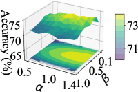
(a)

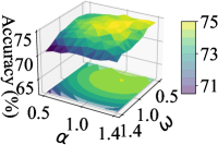
(b)

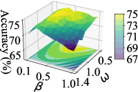
(c)

Figure 5: Sensitivity analysis of hyper-parameters.

C.2 Expanded Model Analysis

Effect of image encoder backbone in CLIP. In this section of the experiment, we examine the impact of the image-encoder backbone in CLIP on the final performance. In addition to the ResNet and ViT-B/32 architectures mentioned in the Experiment Section 4, we also implement ProDe using another well-known architecture, ViT-B/16, which we refer to as ProDe-V16 (the ViT-B/32 version is renamed ProDe-V32). Furthermore, we compare the performance of DAPL-V16, ADCLIP-V16, PAD-V16 and DAMP-V16, which also use ViT-B/16 as their image encoder. As listed in Tab. 12, compared with its variation versions using other backbones, ProDe’s performance is proportional to the representing ability of backbones, as our expectation. Also, ProDe-V16 still surpasses all UDA comparisons. Combining with the ResNet and ViT-B/32 results reported in Tab. 1$\sim$Tab. 2, it is concluded that the advantage of ProDe is robust to the selection of the image-encoder backbone.

Effect of prompt learning. In ProDe, prompt learning contributes to knowledge synchronization. To isolate its effectiveness, we propose a variation method ProDe-V w/o prompt that removes prompt learning. As shown in Tab. 13, absence of prompt learning results in 0.9% decrease in average accuracy.

Parameter sensitivity. In this part, we discuss the parameter sensitivity of parameters $\alpha$, $\beta$ in $L_{ProDe}$ (see Eq. (6)) and correction strength parameter $\omega$ in proxy denoising (see Eq. (5)). All experiments are conducted based on the transfer tasks Cl$\to$Ar in the Office-Home dataset. The varying range are set to $0.5\leq\alpha\leq 1.4$, $0.1\leq\beta\leq 1.0$ and $0.5\leq\omega\leq 1.4$ in 0.1 step size. Fig. 5 (a) depicts the results as $\alpha$–$\beta$ vary. When the two parameters changes, there are no evident drops in the accuracy variation curves, except for two boundary situations: (1) $\alpha=0.5$ and (2) $\beta=1.0$. The results indicate that ProDe is insensitive to parameters $\alpha$ and $\beta$. Meanwhile, when we select parameters, $\alpha$’s value should be lager than $\beta$. Besides, in Fig. 5 (b) and (c), we display the results when $\alpha$–$\omega$ and $\alpha$–$\omega$ vary, respectively. Thus, we present the relation between the correction strength and regularization elements in $L_{ProDe}$. From the two sub-figures, it is seen that the performance has a significant drop as $\omega=1.4$. This show that the correction strength in the proxy denoising block should not be too strong.

Appendix D Limitations

Our method has shown impressive performance in multi-SFDA settings, highlighting its efficacy. However, it is important to note that it is specifically designed for a white-box and offline scenario, which may not be applicable in certain real-world contexts. For the kind of black-box application, such as models in the cloud, our proxy denoising may not work well since all details of the model, including the required logits features, are transparent to us. Additionally, the training supervised by mutual knowledge distilling regularization relies on the dataset prepared in advance, which limits the data flow over time. In the future, finding ways to extend our method to these new scenarios will be an interesting direction.

References

- Andonian et al. [2022] Alex Andonian, Shixing Chen, and Raffay Hamid. Robust cross-modal representation learning with progressive self-distillation. In Proceedings of the IEEE/CVF Conference on Computer Vision and Pattern Recognition, pages 16430–16441, 2022.
- Bai et al. [2024] Shuanghao Bai, Min Zhang, Wanqi Zhou, Siteng Huang, Zhirong Luan, Donglin Wang, and Badong Chen. Prompt-based distribution alignment for unsupervised domain adaptation. In Proceedings of the AAAI Conference on Artificial Intelligence, pages 729–737, 2024.
- Cha et al. [2022] Junbum Cha, Kyungjae Lee, Sungrae Park, and Sanghyuk Chun. Domain generalization by mutual-information regularization with pre-trained models. In European Conference on Computer Vision, pages 440–457. Springer, 2022.
- Chen et al. [2022a] Dian Chen, Dequan Wang, Trevor Darrell, and Sayna Ebrahimi. Contrastive test-time adaptation. In Proceedings of the IEEE/CVF Conference on Computer Vision and Pattern Recognition, pages 295–305, 2022a.
- Chen et al. [2022b] Weijie Chen, Luojun Lin, Shicai Yang, Di Xie, Shiliang Pu, and Yueting Zhuang. Self-supervised noisy label learning for source-free unsupervised domain adaptation. In Proceedings of the IEEE/RSJ International Conference on Intelligent Robots and Systems, pages 10185–10192. IEEE, 2022b.
- Ding et al. [2022] Ning Ding, Yixing Xu, Yehui Tang, Chao Xu, Yunhe Wang, and Dacheng Tao. Source-free domain adaptation via distribution estimation. In Proceedings of the IEEE/CVF Conference on Computer Vision and Pattern Recognition, pages 7212–7222, 2022.
- Du et al. [2023] Yuntao Du, Haiyang Yang, Mingcai Chen, Hongtao Luo, Juan Jiang, Yi Xin, and Chongjun Wang. Generation, augmentation, and alignment: A pseudo-source domain based method for source-free domain adaptation. Machine Learning, pages 1–21, 2023.
- Du et al. [2024] Zhekai Du, Xinyao Li, Fengling Li, Ke Lu, Lei Zhu, and Jingjing Li. Domain-agnostic mutual prompting for unsupervised domain adaptation. Proceedings of the IEEE/CVF International Conference on Computer Vision, 2024.
- Ganin and Lempitsky [2015] Yaroslav Ganin and Victor S. Lempitsky. Unsupervised domain adaptation by backpropagation. In International conference on machine learning, pages 1180–1189, 2015.
- Ge et al. [2022] Chunjiang Ge, Rui Huang, Mixue Xie, Zihang Lai, Shiji Song, Shuang Li, and Gao Huang. Domain adaptation via prompt learning. arXiv:2202.06687, 2022.
- Ghasedi Dizaji et al. [2017] Kamran Ghasedi Dizaji, Amirhossein Herandi, Cheng Deng, Weidong Cai, and Heng Huang. Deep clustering via joint convolutional autoencoder embedding and relative entropy minimization. In Proceedings of the IEEE/CVF International Conference on Computer Vision, pages 5736–5745, 2017.
- Huang et al. [2021] Jiaxing Huang, Dayan Guan, Aoran Xiao, and Shijian Lu. Model adaptation: Historical contrastive learning for unsupervised domain adaptation without source data. Advances in Neural Information Processing Systems, 34:3635–3649, 2021.
- Ji et al. [2019] Xu Ji, Joao F Henriques, and Andrea Vedaldi. Invariant information clustering for unsupervised image classification and segmentation. In Proceedings of the IEEE/CVF International Conference on Computer Vision, pages 9865–9874, 2019.
- Jia et al. [2022] Menglin Jia, Luming Tang, Bor-Chun Chen, Claire Cardie, Serge Belongie, Bharath Hariharan, and Ser-Nam Lim. Visual prompt tuning. In Proceedings of the European Conference on Computer Vision, pages 709–727. Springer, 2022.
- Kang et al. [2019] Guoliang Kang, Lu Jiang, Yi Yang, and Alexander G Hauptmann. Contrastive adaptation network for unsupervised domain adaptation. In Proceedings of the IEEE/CVF Conference on Computer Vision and Pattern Recognition, pages 4893–4902, 2019.
- Kundu et al. [2022] Jogendra Nath Kundu, Akshay R Kulkarni, Suvaansh Bhambri, Deepesh Mehta, Shreyas Anand Kulkarni, Varun Jampani, and Venkatesh Babu Radhakrishnan. Balancing discriminability and transferability for source-free domain adaptation. In International Conference on Machine Learning, pages 11710–11728. PMLR, 2022.
- Kurmi et al. [2021] Vinod K Kurmi, Venkatesh K Subramanian, and Vinay P Namboodiri. Domain impression: A source data free domain adaptation method. In Proceedings of the IEEE/CVF Winter Conference on Applications of Computer Vision, pages 615–625, 2021.
- Lai et al. [2023] Zhengfeng Lai, Noranart Vesdapunt, Ning Zhou, Jun Wu, Cong Phuoc Huynh, Xuelu Li, Kah Kuen Fu, and Chen-Nee Chuah. Padclip: Pseudo-labeling with adaptive debiasing in clip for unsupervised domain adaptation. In Proceedings of the IEEE/CVF International Conference on Computer Vision, pages 16155–16165, 2023.
- Lao et al. [2021] Qicheng Lao, Xiang Jiang, and Mohammad Havaei. Hypothesis disparity regularized mutual information maximization. In Proceedings of the AAAI Conference on Artificial Intelligence, pages 8243–8251, 2021.
- Lee et al. [2022] Jonghyun Lee, Dahuin Jung, Junho Yim, and Sungroh Yoon. Confidence score for source-free unsupervised domain adaptation. In International conference on machine learning, pages 12365–12377. PMLR, 2022.
- Li et al. [2021] Jingjing Li, Zhekai Du, Lei Zhu, Zhengming Ding, Ke Lu, and Heng Tao Shen. Divergence-agnostic unsupervised domain adaptation by adversarial attacks. IEEE Transactions on Pattern Analysis and Machine Intelligence, 44(11):8196–8211, 2021.
- Li et al. [2022] Liunian Harold Li, Pengchuan Zhang, Haotian Zhang, Jianwei Yang, Chunyuan Li, Yiwu Zhong, Lijuan Wang, Lu Yuan, Lei Zhang, Jenq-Neng Hwang, et al. Grounded language-image pre-training. In Proceedings of the IEEE/CVF Conference on Computer Vision and Pattern Recognition, pages 10965–10975, 2022.
- Li et al. [2020a] Rui Li, Qianfen Jiao, Wenming Cao, Hau-San Wong, and Si Wu. Model adaptation: Unsupervised domain adaptation without ource data. In Proceedings of the IEEE/CVF Conference on Computer Vision and Pattern Recognition, pages 9638–9647, 2020a.
- Li et al. [2020b] Rui Li, Qianfen Jiao, Wenming Cao, Hau-San Wong, and Si Wu. Model adaptation: Unsupervised domain adaptation without source data. In Proceedings of the IEEE/CVF conference on computer vision and pattern recognition, pages 9641–9650, 2020b.
- Liang et al. [2023] Feng Liang, Bichen Wu, Xiaoliang Dai, Kunpeng Li, Yinan Zhao, Hang Zhang, Peizhao Zhang, Peter Vajda, and Diana Marculescu. Open-vocabulary semantic segmentation with mask-adapted clip. In Proceedings of the IEEE/CVF Conference on Computer Vision and Pattern Recognition, pages 7061–7070, 2023.
- Liang et al. [2020] Jian Liang, Dapeng Hu, and Jiashi Feng. Do we really need to access the source data? source hypothesis transfer for unsupervised domain adaptation. In Proceedings of the International Conference on Machine Learning, pages 6028–6039, 2020.
- Litrico et al. [2023] Mattia Litrico, Alessio Del Bue, and Pietro Morerio. Guiding pseudo-labels with uncertainty estimation for source-free unsupervised domain adaptation. In Proceedings of the IEEE/CVF Conference on Computer Vision and Pattern Recognition, pages 7640–7650, 2023.
- Liu et al. [2024] Jie Liu, Jinzong Cui, Mao Ye, Xiatian Zhu, and Song Tang. Shooting condition insensitive unmanned aerial vehicle object detection. Expert Systems with Applications, 246:123221, 2024.
- Müller et al. [2019] R. Müller, S. Kornblith, and G. E Hinton. When does label smoothing help? In Advances in Neural Information Processing Systems, pages 4696–4705, 2019.
- Pei et al. [2023] Renjing Pei, Jianzhuang Liu, Weimian Li, Bin Shao, Songcen Xu, Peng Dai, Juwei Lu, and Youliang Yan. Clipping: Distilling clip-based models with a student base for video-language retrieval. In Proceedings of the IEEE/CVF Conference on Computer Vision and Pattern Recognition, pages 18983–18992, 2023.
- Peng et al. [2017] Xingchao Peng, Ben Usman, Neela Kaushik, Judy Hoffman, Dequan Wang, and Kate Saenko. Visda: The visual domain adaptation challenge. arXiv:1710.06924, 2017.
- Peng et al. [2019] Xingchao Peng, Qinxun Bai, Xide Xia, Zijun Huang, Kate Saenko, and Bo Wang. Moment matching for multi-source domain adaptation. In Proceedings of the IEEE/CVF International Conference on Computer Vision, pages 1406–1415, 2019.
- Radford et al. [2021] Alec Radford, Jong Wook Kim, Chris Hallacy, Aditya Ramesh, Gabriel Goh, Sandhini Agarwal, Girish Sastry, Amanda Askell, Pamela Mishkin, Jack Clark, et al. Learning transferable visual models from natural language supervision. In Proceedings of the International Conference on Machine Learning, pages 8748–8763. PMLR, 2021.
- Roy et al. [2022] Subhankar Roy, Martin Trapp, Andrea Pilzer, Juho Kannala, Nicu Sebe, Elisa Ricci, and Arno Solin. Uncertainty-guided source-free domain adaptation. In Proceedings of the European Conference on Computer Vision, pages 537–555. Springer, 2022.
- Saenko et al. [2010] Kate Saenko, Brian Kulis, Mario Fritz, and Trevor Darrell. Adapting visual category models to new domains. In Proceedings of the European Conference on Computer Vision, pages 213–226. Springer, 2010.
- Saito et al. [2019] Kuniaki Saito, Donghyun Kim, Stan Sclaroff, Trevor Darrell, and Kate Saenko. Semi-supervised domain adaptation via minimax entropy. In Proceedings of the IEEE/CVF International Conference on Computer Vision, pages 8050–8058, 2019.
- Singha et al. [2023] Mainak Singha, Harsh Pal, Ankit Jha, and Biplab Banerjee. AD-CLIP: Adapting domains in prompt space using CLIP. In Proceedings of the IEEE/CVF International Conference on Computer Vision Workshop, pages 4355–4364, 2023.
- Tang et al. [2021] S Tang, Yuji Shi, Zhiyuan Ma, Jian Li, Jianzhi Lyu, Qingdu Li, and Jianwei Zhang. Model adaptation through hypothesis transfer with gradual knowledge distillation. In Proceedings of the IEEE/RSJ International Conference on Intelligent Robots and Systems, pages 5679–5685. IEEE, 2021.
- Tang et al. [2021] Song Tang, Yan Yang, Zhiyuan Ma, Norman Hendrich, Fanyu Zeng, Shuzhi Sam Ge, Changshui Zhang, and Jianwei Zhang. Nearest neighborhood-based deep clustering for source data-absent unsupervised domain adaptation. arXiv:2107.12585, 2021.
- Tang et al. [2022] Song Tang, Yan Zou, Zihao Song, Jianzhi Lyu, Lijuan Chen, Mao Ye, Shouming Zhong, and Jianwei Zhang. Semantic consistency learning on manifold for source data-free unsupervised domain adaptation. Neural Networks, 152:467–478, 2022.
- Tang et al. [2024a] Song Tang, An Chang, Fabian Zhang, Xiatian Zhu, Mao Ye, and Changshui Zhang. Source-free domain adaptation via target prediction distribution searching. International journal of computer vision, 132(3):654–672, 2024a.
- Tang et al. [2024b] Song Tang, Yuji Shi, Zihao Song, Mao Ye, Changshui Zhang, and Jianwei Zhang. Progressive source-aware transformer for generalized source-free domain adaptation. IEEE Transactions on Multimedia, 26:4138–4152, 2024b.
- Tang et al. [2024c] Song Tang, Wenxin Su, Mao Ye, and Xiatian Zhu. Source-free domain adaptation with frozen multimodal foundation model. Proceedings of the IEEE/CVF Conference on Computer Vision and Pattern Recognition, 2024c.
- Tanwisuth et al. [2021] Korawat Tanwisuth, Xinjie Fan, Huangjie Zheng, Shujian Zhang, Hao Zhang, Bo Chen, and Mingyuan Zhou. A prototype-oriented framework for unsupervised domain adaptation. pages 17194–17208, 2021.
- Tian et al. [2021] Jiayi Tian, Jing Zhang, Wen Li, and Dong Xu. Vdm-da: Virtual domain modeling for source data-free domain adaptation. IEEE Transactions on Circuits and Systems for Video Technology, 32(6):3749–3760, 2021.
- Tian et al. [2022] Jiayi Tian, Jing Zhang, Wen Li, and Dong Xu. Vdm-da: virtual domain modeling for source data-free domain adaptation. IEEE Trans. Circuits Syst. Video Technol., 32(6):3749–3760, 2022.
- Venkateswara et al. [2017] Hemanth Venkateswara, Jose Eusebio, Shayok Chakraborty, and Sethuraman Panchanathan. Deep hashing network for unsupervised domain adaptation. In Proceedings of the IEEE/CVF Conference on Computer Vision and Pattern Recognition, pages 5385–5394, 2017.
- Wang et al. [2022a] Fan Wang, Zhongyi Han, Yongshun Gong, and Yilong Yin. Exploring domain-invariant parameters for source free domain adaptation. In Proceedings of the IEEE Conference on Computer Vision and Pattern Recognition, pages 7151–7160, 2022a.
- Wang et al. [2021] Jue Wang, Haofan Wang, Jincan Deng, Weijia Wu, and Debing Zhang. Efficientclip: Efficient cross-modal pre-training by ensemble confident learning and language modeling. arXiv preprint arXiv:2109.04699, 2021.
- Wang et al. [2023] Yan Wang, Jian Cheng, Yixin Chen, Shuai Shao, Lanyun Zhu, Zhenzhou Wu, Tao Liu, and Haogang Zhu. Fvp: Fourier visual prompting for source-free unsupervised domain adaptation of medical image segmentation. IEEE Transactions on Medical Imaging, 2023.
- Wang et al. [2022b] Zhaoqing Wang, Yu Lu, Qiang Li, Xunqiang Tao, Yandong Guo, Mingming Gong, and Tongliang Liu. CRIS: Clip-driven referring image segmentation. In Proceedings of the IEEE/CVF conference on computer vision and pattern recognition, pages 11686–11695, 2022b.
- Xia et al. [2021] Haifeng Xia, Handong Zhao, and Zhengming Ding. Adaptive adversarial network for source-free domain adaptation. In Proceedings of the IEEE/CVF International Conference on Computer Vision, pages 9010–9019, 2021.
- Xu et al. [2019] Ruijia Xu, Guanbin Li, Jihan Yang, and Liang Lin. Larger norm more transferable: An adaptive feature norm approach for unsupervised domain adaptation. In Proceedings of the IEEE/CVF International Conference on Computer Vision, pages 1426–1435, 2019.
- Yang et al. [2021a] Shiqi Yang, Joost van de Weijer, Luis Herranz, Shangling Jui, et al. Exploiting the intrinsic neighborhood structure for source-free domain adaptation. pages 29393–29405, 2021a.
- Yang et al. [2021b] Shiqi Yang, Yaxing Wang, Joost Van De Weijer, Luis Herranz, and Shangling Jui. Generalized source-free domain adaptation. In Proc. IEEE Int. Conf. Comput. Vis. (ICCV), pages 8978–8987, 2021b.
- Yang et al. [2022] Shiqi Yang, Yaxing Wang, Kai Wang, Shangling Jui, et al. Attracting and dispersing: A simple approach for source-free domain adaptation. In Advances in Neural Information Processing Systems, 2022.
- Yi et al. [2023] Li Yi, Gezheng Xu, Pengcheng Xu, Jiaqi Li, Ruizhi Pu, Charles Ling, A Ian McLeod, and Boyu Wang. When source-free domain adaptation meets learning with noisy labels. nternational Conference on Learning Representations, 2023.
- Zhang et al. [2023] Yixin Zhang, Zilei Wang, and Weinan He. Class relationship embedded learning for source-free unsupervised domain adaptation. In Proceedings of the IEEE/CVF Conference on Computer Vision and Pattern Recognition, pages 7619–7629, 2023.
- Zhou et al. [2022] Kaiyang Zhou, Jingkang Yang, Chen Change Loy, and Ziwei Liu. Learning to prompt for vision-language models. International Journal of Computer Vision, 130(9):2337–2348, 2022.
- Zhou et al. [2024] Lihua Zhou, Nianxin Li, Mao Ye, Xiatian Zhu, and Song Tang. Source-free domain adaptation with class prototype discovery. Pattern recognition, 145:109974, 2024.