Generalized phase estimation in noisy quantum gates
Abstract
We examine metrological scenarios where the parameter of interest is encoded onto a quantum state through the action of a noisy quantum gate and investigate the ultimate bound to precision by analyzing the behaviour of the Quantum Fisher Information (QFI). We focus on qubit gates and consider the possibility of employing successive applications of the gate. We go beyond the trivial case of unitary gates and characterize the robustness of the metrological procedure introducing noise in the performed quantum operation, looking at how this affects the QFI at different steps (gate applications). We model the dephasing and tilting noise affecting qubit rotations as classical fluctuations governed by a Von Mises-Fisher distribution. Compared to the noiseless case, in which the QFI grows quadratically with the number of steps, we observe a non monotonic behavior, and the appearance of a maximum in the QFI, which defines the ideal number of steps that should be performed in order to precisely characterize the action of the gate.
I Introduction
Quantum Estimation Theory [1] is the mathematical framework providing the optimal methodologies to asses the precision in the estimation of one or more parameters encoded in the state of a quantum system. Phase Estimation [2], in particular, is attracting great attention because of its importance not only in metrology [3, 4, 5] but also in quantum information processing in general [6, 7, 8, 9]. Here we consider the case in which the parameter to be estimated is encoded in the transformation associated to a quantum gate acting on a qubit [10, 11]. The typical metrological procedure is to prepare an initial state independent from the parameter, apply the quantum gate (one or many times) and then perform a measurement to extract information about the unknown value of the parameter(s).
In the ideal case of unitary gate operation, the metrological procedure may be easily optimized [12], whereas in the presence of noise the problem is not trivial and has not been fully addressed so far. In turn, the current generation of noisy intermediate-scale quantum devices (NISQ), and likely those in the near future, [13, 14] are unavoidably affected by noise. The noise affecting NISQ may be classified in different categories [15], including gate infidelities [16], state preparation and measurement (SPAM) errors [17], decoherence resulting from the interaction with the environment,[18] and dephasing of the physical qubits. Gate imperfections may be modeled as generalized depolarizing channels [19, 20], i.e., assigning probabilities to the operations described by the Pauli X,Y and Z gates. Another approach is to forget any information about the gate and set an estimation procedure in which this is not required[21]. In this case, doubling the dimension of the probe system and using an an entangled initial state, it is possible to retrieve a relevant amount of information about the parameter [22, 23, 24].
In this paper, we address realistic noise affecting the transformation performed by the gate, regardless of the causes. In particular, the actual transformation could be different from the one we wanted to apply, and we model the noisy transformation as a weighted sum over all the possible transformations [25, 24, 26]. Since every unitary transformation on a qubit can be seen as a rotation of its Bloch vector, we consider two types of noise: one affecting the angle of rotation, referred to as dephasing noise [27, 28], and the other one affecting the rotation axis, referred to as tilting noise. The transformations obtained through this procedure cease to be unitary, and we analyze how this affects the estimation of the gate phase parameter compared to the ideal case. In order to quantify the precision attainable in the estimation of a single parameter , a lower bound is provided by the quantum Crameŕ-Rao theorem, stating
| (1) |
where is the number of measurements available and is a quantity called Quantum Fisher Information (QFI). This tells us that the precision can be arbitrarily increased by increasing the number of measuremets. However, this comes with a cost, and in order to exploit each measurement as much as possible we should look at the conditions maximizing . In the following, we analyze in details how the dephasing and tilting noise affect the QFI of the phase parameter encoded on the qubit by the gate.
The paper is structured as follow. In Sec.II, we review the mathematical tools needed for the characterization of the noisy quantum gates. In Sec.III, we evaluate the temporal evolution of the quantum state undergoing successive gate applications. In Sec.IV, we illustrate the results obtained for the two types of noise, and seek for the optimal number of gate applications that enhances the metrological performance of our system. Finally, Sec.V closes the paper with some concluding remarks. Additional material can be found in Appendices A-B.
II Metrology on the Bloch sphere
The most general qubit state may be written as
| (2) |
and may be associated to a vector on the unit sphere, usually referred to as Bloch vector: . For mixed states , the Bloch vector is obtained by
| (3) |
where is the vector of Pauli matrices:
| (4) |
A quantum gate encodes a transformation performed on a quantum state. To map pure states to pure states (as the evolution of a quantum isolated state should do) the corresponding matrix must be unitary: since we are acting on a qubit. However, we will consider only special unitary matrices: , because every unitary matrix can be written as a special unitary times a phase, whose action is trivial on a quantum state. A unitary transformation acting on a qubit corresponds to a rotation of its Bloch vector. To see this we write by exponentiation of the generators: with being the generalized angles [29]. It transforms a state as . Taking first order of an infinitesimal rotation
| (5) |
the corresponding Bloch vector is transformed as
| (6) |
so that the (special) unitary transformation corresponds to the rotation , around the axis .
In parameter estimation, the goal is to estimate the value of a parameter by sampling a stochastic variable , whose conditional distribution is the probability to obtain outcome provided that the the parameter has value . A fundamental result is the Cramér-Rao inequality [30, 31], providing a lower bound on the variance of when it is by measuring the variable :
| (7) |
The difference with Eq.(1) is that in the right hand side we have , termed Fisher Information (FI), defined as
| (8) |
In a quantum mechanical framework would be a parameter of a quantum state. Measurements are performed through positive operators (POVM) with , and can be seen as tools to generate the probability distributions . In this way, some measurements will generate probability distributions with a high FI while others will be less efficient. By maximizing the FI with respect of all the possible measurements one obtains the the quantum Cramér-Rao bound [32] of Eq.(1), having then
| (9) |
In this way, the QFI depends only on the quantum state and is defined as
| (10) |
where is an hermitian operator, referred to as the Symmetric Logarithmic Derivative (SLD). It is related to the rate at which the state changes when varies and is implicitly defined as
| (11) |
Evaluating the QFI for a quantum state gives an upper bound on the precision, which may be achieved by measuring the projectors on the eigenstates of the SLD operator.
The evaluation of usually involves the diagonalization of the state density matrix. For qubits this leads to [33, 34]
| (12) |
where is the Bloch vector associated to the state .
The Cramér-Rao theorem is valid for those values of the parameter where the QFI is continuous, otherwise the bound does not hold [35, 36]. In the quantum case, discountinuities usually occur at values of the parameter for which the rank of the density matrix changes. In our case, this happens for , and therefore we consider the domain . This happens because for the rotation around any axis is the identity and is left invariant by any form of noise, while for fluctuations of turn any unitary rotation into a purity decreasing quantum operation.
Since we want to characterize a noisy system where the parameter is the rotation amplitude around a given rotation axis, the fluctuations of those parameters happen on a circular or spherical domain. A convenient distribution is thus given by the von Mises-Fisher probability density function [37], defined as
| (13) |
where are vectors belonging to the sphere and is a normalization factor that depends on the dimension
| (14) |
with denoting the modified Bessel function of the first kind of order evaluated at . The quantity identifies the predominant direction on the hypersphere while represents a concentration parameter, and controls how fast the probability decreases when deviates from .
For we are considering a stochastic variable living on a circle and the corresponding density function, known as von Mises distribution, reduces to
| (15) |
An alternative expression in series of cosines is given by
| (16) |
The case was introduced [38] to provide the correct distribution for elementary errors over the surface of the unit sphere, pointing out that the most used Gaussian distribution loses validity when the entity of the errors forces to consider the actual topology. The probability density reads
| (17) |
III The statistical model
We address a parameter estimation problem in which the dependence on the parameter is encoded onto a quantum state by the application of a -dependent quantum gate. In particular, we consider the scenario in which the quantum gate, due to imperfections leading to fluctuations, instead of performing the desired transformation may perform a different one. Let us denote by the intended transformation and the possible transformations that are actually performed. Here denotes a -dimensional parameter () so that runs over a certain subset of the matrices. The gate performs the transformation with probability , with . If is the the initial state of the qubit, after gate iterations, we are left with the state
| (18) |
The quantity is discrete and denotes the number of gate iterations. We nevertheless refer to as the ’time’. The Bloch vector at time is given by
| (19) |
where is the Bloch rotation corresponding to . If we assume that the probability distribution is the same at each gate iteration and is independent on the state on which the gate acts, linearity allows us to write
| (20) | ||||
| (21) |
This tells us that once we compute the ‘noisy rotation’
| (22) |
we can simply apply it to the initial Bloch vector to obtain the evolved one at each gate iteration. Alternatively, we may also use the following expressions [39]
| (23) | ||||
| (24) |
where
| (25) |
Once we know and we can compute the QFI at time .
IV Results
In this Section, we illustrate results. We start by considering systems affected by pure dephasing, i.e., noise affecting only the angle of rotation, and then examine the case of pure tilting, where noise is affecting only the axis of rotation. Finally, we consider the general case where both kind of noise are present. Notice that this is the most general kind of noise that may occur for a qubit rotation, which is characterized by the degrees of freedom of a 3-dimensional rotation (one for dephasing, and two for tilting). As we will see in details, the presence of noise dramatically alters the behavior of the QFI compared to the noiseless case. The most striking difference being that the QFI does no longer increase indefinitely with the number of gate applications, but instead reaches a maximum and then goes to zero.
IV.1 Noiseless evolution
Let us start with the noiseless case, in which the gate performs exactly the desired operation [40]. Starting from a generic state, we have
| (26) |
We apply times a rotation of an angle , that is the parameter to be estimated. We choose a rotation without loss of generality (see Appendix A)
| (27) |
and after iterations the state is
| (31) |
Using Eq.(12) it is easy to obtain
| (32) |
The QFI increases with the purity of the initial state, which is not spoiled by the simple rotation applied. Indeed, as observed in [34], the QFI always increases with the purity of the measured qubit state. In addition, we see that the QFI grows quadratically with the number of gate iterations, and depends on the polar angle of the initial state through a factor . This is in accordance with a well known result [41], stating that when the dependence on a parameter is given to a quantum state through the action of a unitary transformation , the QFI is maximized by taking the initial state in the form , where and are the eigenstates of the generator of the transformation associated to the highest and lowest eigenvalues. Here the generator would be proportional to the Pauli matrix , whose eigenstates are the elements of the trivial basis and . An equal superposition of them would lie on the equator of the Bloch sphere, having then . Interestingly, the QFI does not depend from the actual rotation angle that we want to estimate.
IV.2 Pure Dephasing
After the analysis of the noiseless evolution we move to the study of the effect of the different noise models. In this Section, we assume that the noise is affecting only the rotation, while the axis of rotation is preserved. In other words, we assume that the gate instead of performing the rotation , may perform the rotation with probability
where denotes the modified Bessel function of the first kind of order . We consider the axis of rotation to be the direction to simplify the computation, but the results hold general by simply rotating the initial vector (see Appendix A). The probability of obtaining a certain rotation is governed by a Von Mises distribution centered in (i.e., we assume an unbiased gate where the most likely rotation is the nominal one) with concentration parameter . This quantity determines the quality of the quantum gate: for we recover the noiseless result, while for the angle of rotation becomes completely random.
The resulting dephased rotation is (see Appendix B)
| (33) |
where . The operation is still rotating the qubit, but also shrinking the Bloch vector in the plane. Indeed, the main difference between a pure and a noisy rotation affected by dephasing stays in the coefficient , which assesses the precision of the operation, according to the limit
| (34) |
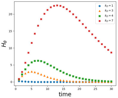
The QFI after gate applications (see Appendix B) is given by
| (35) |
The behaviour of as a function of the number of gate applications is shown in Fig. 1 for different values of the concentration parameter . We see that noise introduces a non-monotonic behavior depending on the ratio , physically motivated by the fact that the gate gives to the state dependence from , but also decreases its purity. Knowing this, it is interesting to find the ideal time , namely the one maximizing Eq.(35).
The optimal value of is given by
| (36) |
Of course, since it represents a number of gate applications, we have to select the closest integer to . Concerning the initial state, the QFI is still maximized taking the starting vector lying on the equator. We see also that, as in the noiseless case, the QFI does not depend on the rotation angle .
IV.3 Pure Tilting
After the analytical characterization of the dephasing case, in this Section we address the case where the noise is affecting only the axis of rotation, preserving the rotation angle . In other words, we assume that the gate, instead of performing the target rotation , is applying the rotation with a probability density given by the Von Mises-Fisher distribution on the 2-Sphere, i.e.,
where . The probability density has concentration parameter and is centered in the direction of the axis (again without loss of generality, see Appendix A). We refer to it as the ”central axis”, because ”rotation axis” would be misleading since we are rotating around all the possible ones. Following the computation in Appendix B, one obtains the tilted rotation , shown in Eq. (68). As expected, we recover a pure rotation in the limit . On the other hand, for vanishing one obtains a transformation proportional to the identity
| (37) |
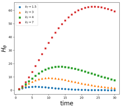
This case, termed uniform tilting, will be treated later. Except for this case, the general expression of becomes cumbersome, as that of the QFI, and will not be reported here. Rather, in Fig. 2 we show the behaviour of the QFI as a function of the number of applications of a tilted rotation for different values of the concentration parameter . As it is apparent from the plot, the behavior is qualitatively similar to the one obtained for dephasing noise: increasing the concentration parameter increases the highest value that is reached by the QFI.
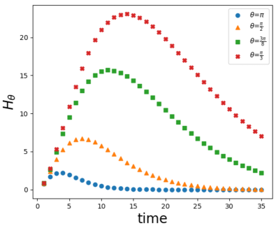
However, despite the similarities with the dephasing noise case, tilting noise introduces a dependence in the QFI from the rotation angle . In particular, as we can see in Fig. 3, the QFI achieves higher values for small rotation angles, where the effect of tilting noise is apparently reduced. The case in which we have no control at all on the axis of rotation can be treated analytically. Indeed, in this case the noisy transformation is that of Eq. (37) which can be obtained computing
| (38) |
Correspondingly, one has
| (39) | ||||
| (40) |
and using Eq.(12),
| (41) |
where
It is interesting to analyze the case in which the initial state is pure (=1). In this case, if , we obtain a linear dependence on time:
| (42) |
We should note that in this case our model falls into the one addressed in [21], where they considered one single gate application. Using two entangled qubits they recovered the maximum value of QFI (), while using an entangle-free couple of qubits they set up a measurement procedure resulting in a FI of regardless of the rotation angle. In our case instead, using a single qubit probe, the QFI in Eq.(41) depends on the rotation angle , and for reads
| (43) |
which assumes its maximum for .
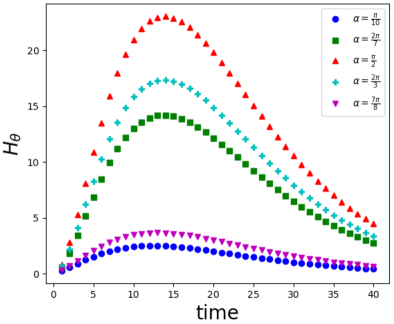
Concerning the dependence from the initial state (in particular from its polar angle ), the highest value of the the QFI is still reached selecting an initial vector lying on the equator of the Bloch sphere (having ) as we can see in Fig. 4. However, the dependence from is not anymore a simple factor.
IV.4 General Noise
As already mentioned, the most general effect of the noise is a combination of both a tilting and dephasing. The gate performs the rotation instead of the desired , where dephasing noise is responsible for fluctuations in the rotation angle uncertainty and the tilting one for the axis instability. The probability governing the fluctuations of the rotation angle is a Von Mises distribution centered in with concentration parameter . The tilting noise is described by a Von Mises-Fisher distribution centered in the central axis , with concentration parameter . The noisy rotation is obtained in B and shown in 73.
As intuitively expected, in the noiseless limit () we recover a pure rotation. Removing the dephasing noise () leaves us with a tilted rotation and thus for we recover a dephased rotation . Contrariwise , in the limit , we no longer have a dependence on , resulting in a vanishing QFI. For while keeping , the QFI assumes the form
| (44) |
where here the quantity in Eq. (41) becomes
This is analogous to the uniform tilting studied in the previous section, but with additional factors which cause
| (45) |
unless we perform the limit in advance. In the general case, the characterization of is more challenging, since it depends on several parameters: and the angle between the central axis and the initial state. For this reason we assume to start with a pure state and focus on two interesting cases.
As a first example, we consider an equatorial initial state with , which is optimal for pure dephasing and pure tilting. We observe again a maximum at a certain time and then a slow decrease. The lower are the noises effect (i.e.m the higher their concentration parameters) the higher is the maximum and also the time at which it is achieved. Still, we see that lowering the actual angle of rotation makes the QFI to increase, approaching the curve we would obtain with pure dephasing (we recall that sending to zero is a way to annihilate the effect of the tilting noise). A remarkable phenomenon also appears for below a certain threshold: there is a crossing between the tails of the pure dephasing noise and the general noise curves. Despite the highest value is always reached by the pure dephasing curve, having a little tilting noise makes the QFI to decrease slower for an increasing number of applications of the gate (see Fig. 5).
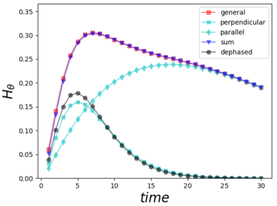
As a second example, we consider a polar initial state, a qubit with . In this case, we first notice that the QFI is much smaller than the one obtained for , but this regime is still interesting for the appearance of a peculiar metrological behavior: if we split in the two components and along the central axis and perpendicular to it, the total QFI is well approximated by the sum of the two QFIs obtained starting with the initial states and , resepctively. The first contribution follows the same behavior of the case. In particular, it is nearly equal to the pure dephasing curve when the tilting noise is very low. The other contribution, instead, can stay much above the pure dephasing curve. For this reason we can find configurations (typically for ) where the QFI for general noise is way higher than the pure dephasing one. This means that in this situations is better to have also a small tilting noise than just the dephasing (see Fig. 5).
V Summary and conclusions
In this paper, we have analyzed the time evolution of a qubit undergoing different noisy quantum gates with the aim of maximizing the Quantum Fisher Information (QFI) associated to the angle of rotation, i.e. to optimize the characterization of the gates themselves. We have employed Bloch notation for the state at step , and described the gate as a non unitary quantum operation depending only on the gate parameter . Since every qubit gate can be seen as a rotation, the noise can be seen as composed of two different sources of fluctuations: deviations from the desired rotation axis (tilting), and fluctuations around the desired value of the rotation angle (dephasing).
Both type of noise have been described as classical fluctuations governed by a Von Mises-Fisher distribution that quantifies the deviation(s) from the desired rotation. We have initially studied the effect of the two noise contribution separately and found that pure dephasing does not introduce dramatic differences compared to the ideal case. In particular, the QFI of does not depend on itself, and is still maximized selecting a pure initial state that is orthogonal to the rotation axis. For pure tilting, instead, the QFI depends on the parameter, favouring small rotation angles. We have then considered the occurrence of both noises at the same time to describe the most general scenario. In this case, we have found situations in which the presence of tilting is beneficial, as it makes the dephasing noise less detrimental.
Overall, compared to the noiseless case, in which the QFI grows quadratically with the number of steps, we have found that the presence of noise leads to a non monotonic behavior, and to the appearance of a maximum in the QFI. In other words, there exists an optimal number of steps (i.e., number of gate applications) to be used in order to precisely characterize the action of the gate.
Acknowledgements.
This work has been done under the auspices of GNFM-INdAM and has been partially supported by MUR and EU through the projects PRIN22-2022T25TR3-RISQUE and PRIN22-PNRR-P202222WBL-QWEST. The authors thank Andrea Secchi for fruitful discussions about the impact of noise on the QFI.Appendix A Proof that one can consider rotations only without loss of generality
Throughout the paper, we often choose to work with rotations. We show here that the case concerning a general axis can be then obtained in a straightforward way. For standard rotations, a simple change of basis gives this relation
| (46) |
where is the rotation bringing the axis into the axis :
| (47) |
Of course it acts in the other way around on rotations, transforming a rotation in a rotation.
It is trivial to show that this is true also when considering a noisy rotation affected by dephasing:
| (48) |
For the tilting case we have that
| (49) |
then
| (50) |
We can choose to integrate in () such that and so . We have then
| (51) |
and so
| (52) |
Given this, it is trivial to show that it is still valid when both tilting and dephasing are considered. This tells us that the noisy rotations related to a general axis are obtained by simply rotating the ones obtained for the axis. So, the initial vector will evolve as
| (53) |
We can also show that, thanks to rotational symmetry, it suffices to compute the QFI for the case. Indeed, the QFI after applications of the noisy gate on the initial vector is
| (54) |
where we used the fact that a rotation such does nothing when acting inside a modulus square or on both factors of a scalar product. We can clearly see that it’s the same QFI we would have obtained for the case, but acting on a different initial vector .
Appendix B Noisy rotation matrices
Here we show the computation required to obtain the noisy rotation matrices and, just for the dephasing noise, the expression of the QFI.
B.1 Dephasing noise
We want to compute the ”noisy rotation” in the case in which the noise affects just the angle of rotation, preserving the axis. Following the prescription of eq.(22) we write
| (55) |
recalling that with we denote the modified Bessel function of order . Expanding the Von Mises distribution as in eq.(16) we get
| (56) |
By expanding also the sines and cosines we will have only integrals of these types
resulting in the pure dephasing noisy matrix
| (57) |
So, starting with the initial vector , after applications of the noisy gate we are left with
| (58) |
Similarly to the noiseless case, , and using eq.(12) we find
| (59) |
B.2 Tilting noise
Here we show how to obtain the ”noisy rotation” matrix in the case of pure tilting noise. According to eq.(22), we need to integrate a rotation around a random axis with a Von Mises Fisher probability density centered on . If we write the rotation axis in polar coordinates we have
| (60) |
Here is the concentration parameter related to the Von Mises Fisher probability distribution and the 3D rotation can be written as
| (61) |
By means of the integrals
| (62) | |||
| (63) | |||
| (64) |
we can get the noisy rotation for pure tilting
| (68) |
where , , .
B.3 General noise
Here instead we assume that noise affects both the axis and the angle of rotation. Similarly to what we did above, we compute the noisy rotation matrix, this time integrating over all the three degrees of freedom of a 3-dimensional rotation.
| (69) |
where and are the concentration parameters of the probability distributions relating the dephasing and tilting noise respectively. Performing the integrals one obtains
| (73) |
where .
References
- Helstrom [1969] C. W. Helstrom, Journal of Statistical Physics 1, 231 (1969).
- Pezzè and Smerzi [2021] L. Pezzè and A. Smerzi, PRX Quantum 2, 040301 (2021).
- Giovannetti et al. [2006] V. Giovannetti, S. Lloyd, and L. Maccone, Physical review letters 96, 010401 (2006).
- Cronin et al. [2009] A. D. Cronin, J. Schmiedmayer, and D. E. Pritchard, Reviews of Modern Physics 81, 1051 (2009).
- Pitkin et al. [2011] M. Pitkin, S. Reid, S. Rowan, and J. Hough, Living Reviews in Relativity 14, 1 (2011).
- Shor [1994] P. W. Shor, in Proceedings 35th annual symposium on foundations of computer science (Ieee, 1994) pp. 124–134.
- Russo et al. [2021] A. E. Russo, K. M. Rudinger, B. C. Morrison, and A. D. Baczewski, Physical review letters 126, 210501 (2021).
- O’Brien et al. [2021] T. E. O’Brien, S. Polla, N. C. Rubin, W. J. Huggins, S. McArdle, S. Boixo, J. R. McClean, and R. Babbush, PRX Quantum 2, 020317 (2021).
- O’Brien et al. [2019] T. E. O’Brien, B. Tarasinski, and B. M. Terhal, New Journal of Physics 21, 023022 (2019).
- Rudinger et al. [2017] K. Rudinger, S. Kimmel, D. Lobser, and P. Maunz, Phys. Rev. Lett. 118, 190502 (2017).
- Lu et al. [2020] H.-H. Lu, Z. Hu, M. S. Alshaykh, A. J. Moore, Y. Wang, P. Imany, A. M. Weiner, and S. Kais, Advanced Quantum Technologies 3, 1900074 (2020).
- Dorner et al. [2009] U. Dorner, R. Demkowicz-Dobrzanski, B. J. Smith, J. S. Lundeen, W. Wasilewski, K. Banaszek, and I. A. Walmsley, Physical review letters 102, 040403 (2009).
- Cheng et al. [2023] B. Cheng, X.-H. Deng, X. Gu, Y. He, G. Hu, P. Huang, J. Li, B.-C. Lin, D. Lu, Y. Lu, et al., Frontiers of Physics 18, 21308 (2023).
- Preskill [2018] J. Preskill, Quantum 2, 79 (2018).
- Georgopoulos et al. [2021] K. Georgopoulos, C. Emary, and P. Zuliani, Physical Review A 104, 062432 (2021).
- Sutherland et al. [2022] R. T. Sutherland, Q. Yu, K. M. Beck, and H. Häffner, Physical Review A 105, 022437 (2022).
- Yu and Wei [2023] H. Yu and T.-C. Wei, arXiv preprint arXiv:2310.18881 (2023).
- Shnirman et al. [2002] A. Shnirman, Y. Makhlin, and G. Schön, Physica Scripta 2002, 147 (2002).
- Chapeau-Blondeau [2016] F. Chapeau-Blondeau, Phys. Rev. A 94, 022334 (2016).
- Chapeau-Blondeau [2024] F. Chapeau-Blondeau, Electronics 13, 439 (2024).
- Song et al. [2024] X. Song, F. Salvati, C. Gaikwad, N. Y. Halpern, D. R. Arvidsson-Shukur, and K. Murch, arXiv preprint arXiv:2403.00054 (2024).
- D’Ariano et al. [2001] G. M. D’Ariano, P. L. Presti, and M. G. A. Paris, Physical review letters 87, 270404 (2001).
- Gillard et al. [2017] N. Gillard, E. Belin, and F. Chapeau-Blondeau, in Actes du GRETSI sur le Traitement du Signal et des Images (2017).
- Rossi and Paris [2015] M. A. Rossi and M. G. A. Paris, Physical Review A 92, 010302 (2015).
- Benedetti and Paris [2014] C. Benedetti and M. G. A. Paris, Physics Letters A 378, 2495 (2014).
- Ferraro et al. [2022] E. Ferraro, D. Rei, M. G. A. Paris, and M. De Michielis, EPJ Quantum Technology 9, 1 (2022).
- Brivio et al. [2010] D. Brivio, S. Cialdi, S. Vezzoli, B. T. Gebrehiwot, M. G. Genoni, S. Olivares, and M. G. A. Paris, Phys. Rev. A 81, 012305 (2010).
- Teklu et al. [2009] B. Teklu, S. Olivares, and M. G. A. Paris, Journal of Physics B: Atomic, Molecular and Optical Physics 42, 035502 (2009).
- Cacciatori and Scotti [2022] S. L. Cacciatori and A. Scotti, Universe 8, 492 (2022).
- Cramér [1999] H. Cramér, Mathematical methods of statistics, Vol. 26 (Princeton university press, 1999).
- Rao [1947] C. R. Rao, in Mathematical Proceedings of the Cambridge Philosophical Society, Vol. 43 (Cambridge University Press, 1947) pp. 280–283.
- Paris [2009] M. G. A. Paris, International Journal of Quantum Information 7, 125 (2009).
- Zhong et al. [2013] W. Zhong, Z. Sun, J. Ma, X. Wang, and F. Nori, Physical Review A 87, 022337 (2013).
- Chapeau-Blondeau [2015] F. Chapeau-Blondeau, Physical Review A 91, 052310 (2015).
- Šafránek [2017] D. Šafránek, Physical Review A 95, 052320 (2017).
- Seveso et al. [2019] L. Seveso, F. Albarelli, M. G. Genoni, and M. G. A. Paris, Journal of Physics A: Mathematical and Theoretical 53, 02LT01 (2019).
- Kurz et al. [2016] G. Kurz, F. Pfaff, and U. D. Hanebeck, in 2016 19th International Conference on Information Fusion (FUSION) (IEEE, 2016) pp. 2087–2094.
- Fisher [1953] R. A. Fisher, Proceedings of the Royal Society of London. Series A. Mathematical and Physical Sciences 217, 295 (1953).
- Cavazzoni et al. [2024] S. Cavazzoni, L. Razzoli, G. Ragazzi, P. Bordone, and M. G. A. Paris, Physical Review A 109, 022432 (2024).
- Liu et al. [2015] J. Liu, X.-X. Jing, and X. Wang, Scientific reports 5, 8565 (2015).
- Tóth and Vértesi [2018] G. Tóth and T. Vértesi, Physical review letters 120, 020506 (2018).