Variational time reversal for free energy estimation in nonequilibrium steady states

Abstract

Studying the structure of systems in nonequilibrium steady states necessitates tools that quantify population shifts and associated deformations of equilibrium free energy landscapes under persistent currents. Within the framework of stochastic thermodynamics, we establish a variant of the Kawasaki–Crooks equality that relates nonequilibrium free energy corrections in driven systems to heat dissipation statistics along time-reversed relaxation trajectories computable with molecular simulation. Using stochastic control theory, we arrive at a variational approach to evaluate the Kawasaki–Crooks equality and use it to estimate distribution functions of order parameters in overdamped Langevin models of active matter, attaining substantial improvement in accuracy over simple perturbative methods.

I Introduction

The free energy surface is a core concept in statistical physics that shapes our understanding of chemistry, materials science, and biology. An assortment of computer-aided drug discovery [1, 2, 3], materials design [4, 5, 6], and basic science efforts are buttressed by well-worn free energy surface estimation methods [7, 8, 9] based on the assumption that the systems targeted operate at or near thermodynamic equilibrium. However, this assumption is incompatible with modern perspectives that seek to understand how nonequilibrium operating conditions govern the function of driven or living systems and active matter.

This emerging nonequilibrium paradigm calls for new molecular simulation methods that can substantially extend the toolbox available in equilibrium to relevant classes of systems driven far from equilibrium. Efforts to bridge this gap have lead to the development of stratification-based techniques for estimating conformation likelihood profiles along relevant order parameters such as Nonequilibrium Umbrella Sampling [10], Forward Flux Sampling [11], and Weighted Ensemble Simulation [12]. These nonequilibrium methods broadly rely on kinetic details of molecular simulation data to determine steady-state populations from global flux balances, and require a statistically expedient spatial stratification for application to complex systems [13]. Such methods operate independently and often distinctly from existing equilibrium methods. Especially in cases where one is interested in understanding how a free energy surface evolves as a system is driven progressively further from equilibrium, it would be advantageous to have a means to leverage existing equilibrium frameworks to aid in their evaluation.

In this work, we develop nonequilibrium free energy surface estimators from results in stochastic thermodynamics, a rapidly developing theoretical framework that extends familiar thermodynamic notions away from equilibrium [14]. At the heart of this formalism lies the Kawasaki–Crooks equality [15], which we revisit in the current work from an optimal control viewpoint. Our analysis yields a method for asymptotically unbiased, variationally exact free-energy estimation in nonequilibrium steady states, by evaluating their change relative to a reference equilibrium surface. Our implementation draws from state-of-the-art approaches to compute dynamical large deviations [16], reaction rates [17], and local entropy flows in active systems [18].

The text is organized as follows. Section II develops the theory and outlines the computational approach of our proposed method for nonequilibrium FES estimation scheme. Section III illustrates its application to simple driven systems. Finally, Section IV provides concluding remarks.

II Theory and Method

In this section, we employ notions from stochastic thermodynamics, path reweighing, and optimal control theory to arrive at estimators for how the free energy surface along collective coordinates deforms under nonequilibrium driving. The estimators are amenable to evaluation via straightforward molecular simulation and standard post-processing analysis, as seen in later sections.

II.1 Nonequilibrium free energy surfaces

Consider a $n$-dimensional system in thermodynamic equilibrium with a heat bath at temperature $\beta^{-1}$, its configuration $X=(x_{1},\ldots,x_{n})^{\top}$ distributed per the Boltzmann–Gibbs probability measure with density

$$\rho^{\mathrm{eq}}(X)\,=\,\exp\,\bm{[}\beta F^{\mathrm{eq}}-\beta U(X)\bm{]}$$ (1)

induced by the potential energy $U$ on the configuration space $\Omega$. The Helmholtz free energy

$$F^{\mathrm{eq}}\,=\,\textstyle\int_{\Omega}\mathrm{d}X\,\rho^{\mathrm{eq}}(X)\,\bm{[}U(X)+\beta^{-1}\ln\rho^{\mathrm{eq}}(X)\bm{]}$$ (2)

is the minimum energy necessary to prepare the equilibrium system from a collection of independent degrees of freedom [19]. Simultaneously, $F^{\mathrm{eq}}$ is the global minimum of the free energy functional $\mathcal{F}_{U}$, which acts on an arbitrary nonequilibrium probability density $\rho^{\mathrm{neq}}$ supported on $\Omega$ to give

$$\mathcal{F}_{U}(\rho^{\mathrm{neq}}) =\,\textstyle\int_{\Omega}\mathrm{d}X\,\rho^{\mathrm{neq}}(X)\,\bm{[}U(X)+\beta^{-1}\ln\rho^{\mathrm{neq}}(X)\bm{]}$$ (3)

$$=\,\mathcal{F}_{U}(\rho^{\mathrm{eq}})+\beta^{-1}\mathcal{D}_{\mathrm{KL}}(\rho^{\mathrm{neq}}\,\|\,\rho^{\mathrm{eq}})$$

where

$$\mathcal{D}_{\mathrm{KL}}(\rho^{\mathrm{neq}}\,\|\,\rho^{\mathrm{eq}})\,\equiv\,\textstyle\int_{\Omega}\mathrm{d}X\,\rho^{\mathrm{neq}}(X)\ln\dfrac{\rho^{\mathrm{neq}}(X)}{\rho^{\mathrm{eq}}(X)}\,\geq\,0$$ (4)

is the Kullback–Leibler divergence from equilibrium of the state specified by $\rho^{\mathrm{neq}}$. If the latter is a physically realizable nonequilibrium state of the system with potential energy $U$, then $\beta^{-1}\mathcal{D}_{\mathrm{KL}}(\rho^{\mathrm{neq}}\,\|\,\rho^{\mathrm{eq}})$ is the nonequilibrium free energy extractable from the system as it autonomously regresses to thermal equilibrium with the enclosing heat bath [20, 21].

Although insightful as a scalar measure of deviation from equilibrium, the nonequilibrium free energy in Eq. (4) informs little about the structure and conformational stability of a driven system. On the other hand, the free energy surface (FES) has long been useful to assess high-dimensional phenomena in terms of low-dimensional structural features that capture the governing physics [22, 23]. While away from equilibrium such a surface does not encode the same response properties as in equilibrium, it still relays the stability of conformations, or groups of configurations, relative to one another along prescribed order parameters [24]. For an order parameter $R:\Omega\to\mathbb{R}$ mapping onto scalar conformations of a system with configuration density $\rho(X)$, equilibrium or otherwise, the FES at conformation $r$ is simply

$$\beta F(r)\,\equiv\,-\ln P(r)\,=\,-\ln\textstyle\int_{\Omega}\mathrm{d}X\,\delta\bm{(}R(X)-r\bm{)}\,\rho(X)$$ (5)

where $P(r)$ is the likelihood of observing the system in conformation $r$. Numerical methods to accurately estimate the equilibrium FES $F^{\mathrm{eq}}(r)$ up to an additive constant are widespread and readily applicable to complex systems [25, 26, 27, 28, 29]. The extension to nonequilibrium applications entails identifying effective estimators of the FES shift

$$\beta F^{\mathrm{neq}}(r)-\beta F^{\mathrm{eq}}(r)\,=\,-\ln\dfrac{P^{\mathrm{neq}}(r)}{P^{\mathrm{eq}}(r)}$$ (6)

where $P^{\mathrm{neq}}(r)$ is the likelihood of conformation $r$ for a system in its nonequilibrium steady state (NESS), and $P^{\mathrm{eq}}(r)$ is the likelihood of the same conformation absent a driving force. Methods to estimate this shift efficiently are lacking.

II.2 Kawasaki–Crooks equality for $\beta F^{\mathrm{neq}}(r)$

The nonequilibrium FES shift in Eq. (6) can be challenging to estimate in driven systems, because unlike in equilibrium, there is no known closed-form configurational reweighing to unbias importance-sampled configurations along arbitrary order parameters in a NESS. Working within the framework of stochastic thermodynamics, in this section we derive an alternative expression for the nonequilibrium free energy surface shift that transfers the burden of nonequilibrium importance sampling away from configuration space and onto path space, where path sampling methods can be leveraged to great effect as we show in later sections.

We develop the theoretical foundation of our results assuming an overdamped diffusive dynamics with additive noise, but surmise generality to other classical Markovian dynamics in common use throughout the stochastic thermodynamics literature. In our context, the system’s equilibrium measure with configuration density $\rho^{\mathrm{eq}}$ is preserved by the stochastic differential equation (SDE) with unit mobility

$$\mathrm{d}X_{t}=\,-\nabla U(X_{t})\,\mathrm{d}t\,+\,\sqrt{2\smash[t]{\beta^{-1}}}\,\mathrm{d}W_{t}$$ (7)

where the standard $n$-dimensional Wiener process $(W_{t})_{t\geq 0}$ encodes the system’s coupling to its enclosing heat bath and satisfies $\langle W_{t}\rangle=0$ and $\langle W_{t}\cdot W_{s}\rangle=n\min(t,s)$ for $t,s\geq 0$. Likewise, the nonequilibrium steady state density $\rho^{\mathrm{neq}}$ corresponds to the invariant measure of the SDE

$$\mathrm{d}X_{t}=\,\bm{[}f(X_{t})-\nabla U(X_{t})\bm{]}\,\mathrm{d}t\,+\,\sqrt{2\smash[t]{\beta^{-1}}}\,\mathrm{d}W_{t}$$ (8)

where the vector field $f$ is assumed to satisfy $\nabla\cdot f=0$ throughout $\Omega$, ensuring that $\rho^{\mathrm{neq}}$ is not a Boltzmann–Gibbs density [30]. Unless otherwise specified, the SDEs in Eqs. (7) and (8) are both endowed with identical equilibrium initial conditions $X_{0}\sim\rho^{\mathrm{eq}}$ throughout our discussion.

At any time horizon $T$, the SDEs in Eqs. (7) and (8) respectively induce mutually overlapping probability measures $\mathbb{P}^{\mathrm{eq}}$ and $\mathbb{P}^{\mathrm{neq}}$ on path space with relative density [31, thm. 8.6.6]

$$\dfrac{\mathrm{d}\mathbb{P}^{\mathrm{neq}}(\bm{X})}{\mathrm{d}\mathbb{P}^{\mathrm{eq}}(\bm{X})} =\,\exp\,\bm{[}-\beta\mathcal{S}_{T}(\bm{X})\bm{]}$$ (9)

$$=\,\exp\,\bm{\{}-\beta\,\bm{[}\mathcal{T}_{T}(\bm{X})+\mathcal{Q}_{T}(\bm{X})\bm{]}/2\bm{\}}$$

at every sample-path $\bm{X}=(X_{t})_{0\leq t\leq T}$. The path functionals

$$\mathcal{T}_{T}(\bm{X})\, =\,\textstyle\int_{0}^{T}\mathrm{d}t\,\tfrac{1}{2}|f(X_{t})|^{2}-\nabla U(X_{t})\cdot f(X_{t})$$ (10a)

$$\mathcal{Q}_{T}(\bm{X})\, =\,-\textstyle\int_{0}^{T}\mathrm{d}X_{t}\circ f(X_{t})$$ (10b)

are respectively called the traffic and the excess heat [32], with the stochastic integral in the latter functional interpreted in the Stratonovich sense [33, ch. 3.2]. This decomposition separates the change of path measure into symmetric and antisymmetric components under the pathwise time-involution operation $\bm{X}\mapsto\tilde{\bm{X}}\!\equiv(X_{T-t})_{0\leq t\leq T}$, as in

$$\mathcal{T}_{T}(\tilde{\bm{X}})\,=\,\mathcal{T}_{T}(\bm{X})\;\;\text{and}\;\;\mathcal{Q}_{T}(\tilde{\bm{X}})\,=\,-\mathcal{Q}_{T}(\bm{X})\,,$$ (11)

clarifying the role of kinetic quantities in path reweighing theories [34, 35]. The relative density in Eq. (9) between equilibrium and nonequilibrium path measures thus exhibits the time-involution symmetry

$$\exp\,\bm{[}-\beta\mathcal{S}_{T}(\tilde{\bm{X}})\bm{]}\,=\,\exp\bm{\{}-\beta\bm{[}\mathcal{S}_{T}(\bm{X})-\mathcal{Q}_{T}(\bm{X})\bm{]}\bm{\}}\,,$$ (12)

which is an instance of a detailed fluctuation theorem [36, 37].

The above facts allow us to derive a Kawasaki–Crooks equality relating the FES shift $\beta F^{\mathrm{neq}}(r)-\beta F^{\mathrm{eq}}(r)$ in Eq. (6) to an average over nonequilibrium paths starting at order parameter value $r$  [38, 39, 40]. Through a derivation detailed in Appendix A, we obtain

$$\ln\dfrac{P^{\mathrm{neq}}(r)}{P^{\mathrm{eq}}(r)}\,=\,\lim_{T\to\infty}\ln\dfrac{\langle\exp\bm{[}\beta\mathcal{Q}_{T}(\bm{X})\bm{]}\rangle^{\mathrm{neq}}_{r}}{\langle\exp\bm{[}\beta\mathcal{Q}_{T}(\bm{X})\bm{]}\rangle^{\mathrm{neq}}}$$ (13)

where the path average $\langle\cdot\rangle_{r}^{\mathrm{neq}}$ is evaluated against realizations of the nonequilibrium SDE in Eq. (8) initialized per the constrained equilibrium density

$$\rho_{r}^{\mathrm{eq}}(X)\,=\,\delta\bm{(}R(X)-r\bm{)}\,\rho^{\mathrm{eq}}(X)/P^{\mathrm{eq}}(r)$$ (14)

The path average in the denominator of Eq. (13) satisfies the integral fluctuation relation

$$1\,=\,\langle\exp\,\bm{[}\beta\mathcal{Q}_{T}(\bm{X})\bm{]}\rangle^{\mathrm{neq}}\;\;\text{for all}\;\;T>0$$ (15)

for the excess heat $\mathcal{Q}_{T}$, also derived in Appendix A. Comparing Eq. (13) with Eq. (6), we observe that the Kawasaki–Crooks equality effectively replaces the constrained nonequilibrium average in the definitional FES shift with a path-integral reweighing of its equilibrium counterpart.

Though more computationally appealing than Eq. (6), the Kawasaki–Crooks FES shift in Eq. (13) involves exponential averages of path observables with time-extensive fluctuations, which can be challenging to estimate despite substantial advancements in enhanced path-sampling methods [41, 42, 43]. Combining Girsanov’s theorem [31, thm. 8.6.6] with Jensen’s inequality [44, thm. 1.6.2] allows us to unpack the Kawasaki–Crooks result in ways that reveal physical insight and reduce numerical variance. For instance, a cumulant expansion to leading order in the excess heat yields

$$\ln\dfrac{P^{\mathrm{neq}}(r)}{P^{\mathrm{eq}}(r)} \approx\,\lim_{T\to\infty}\bm{[}\langle\beta\mathcal{Q}_{T}(\bm{X})\rangle^{\mathrm{neq}}_{r}-\langle\beta\mathcal{Q}_{T}(\bm{X})\rangle^{\mathrm{neq}}\bm{]}$$ (16)

$$\equiv\,\beta F^{\mathrm{eq}}(r)-\beta\hat{F}^{\mathrm{neq}}_{\mathcal{Q}}(r)$$

where $\hat{F}^{\mathrm{neq}}_{\mathcal{Q}}(r)$ is a heat-based estimate of the nonequilibrium FES. To leading order, then, nonequilibrium free energy shifts arise at order parameter values $r$ from which a large amount of excess heat is dissipated as the system is driven from equilibrium towards its nonequilibrium steady state [39, 21, 45, 46]. Alternatively, a reweighing of the averages in Eq. (13) into the equilibrium path ensemble with measure $\mathbb{P}^{\mathrm{eq}}$ followed by expansion up to leading order yields

$$\ln\dfrac{P^{\mathrm{neq}}(r)}{P^{\mathrm{eq}}(r)} =\,\lim_{T\to\infty}\ln\dfrac{\langle\exp\,\bm{[}-\beta(\mathcal{S}_{T}-\mathcal{Q}_{T})(\bm{X})\bm{]}\rangle^{\mathrm{eq}}_{r}}{\langle\exp\,\bm{[}-\beta(\mathcal{S}_{T}-\mathcal{Q}_{T})(\bm{X})\bm{]}\rangle^{\mathrm{eq}}}$$ (17)

$$\approx\,\lim_{T\to\infty}\bm{[}\langle\beta\mathcal{T}_{T}(\bm{X})\rangle^{\mathrm{eq}}-\langle\beta\mathcal{T}_{T}(\bm{X})\rangle^{\mathrm{eq}}_{r}\bm{]}/2$$

$$\equiv\,\beta F^{\mathrm{eq}}(r)-\beta\hat{F}^{\mathrm{neq}}_{\mathcal{T}}(r)$$

or a traffic-based estimate of the free energy surface, $\hat{F}^{\mathrm{neq}}_{\mathcal{T}}(r)$. This result is related to nonlinear response theory for NESSs [34, 47, 35] and has been used to estimate nonequilibrium population shifts with equilibrium averages of time-reversal symmetric trajectory observables [48].

II.3 Variational time reversal estimation of $\beta F^{\mathrm{neq}}(r)$

FES estimates $\hat{F}^{\mathrm{neq}}_{\mathcal{Q}}(r)$ in Eq. (16) and $\hat{F}^{\mathrm{neq}}_{\mathcal{T}}(r)$ in Eq. (17), although appealing for their simplicity, can yield highly biased estimates of the Kawasaki–Crooks FES shift in Eq. (13) under strong driving [49, ch. 5]. Stochastic optimal control arguments yield a variational estimator for the exponential average in Eq. (13) by introducing a guiding field or control policy $\varv_{\bm{\theta}}$ into the nonequilibrium dynamics, resulting in

$$\lim_{T\to\infty}\ln\,\langle\exp\,\bm{[}\beta\mathcal{Q}_{T}(\bm{X})\bm{]}\rangle_{r}^{\mathrm{neq}}$$ (18)

$$\qquad\,=\,\lim_{T\to\infty}\ln\,\Bigl{\langle}\exp\,\bm{[}\beta\mathcal{Q}_{T}(\bm{X})\bm{]}\dfrac{\mathrm{d}\mathbb{P}^{\mathrm{neq}}(\bm{X})}{\mathrm{d}\mathbb{P}^{\varv_{\bm{\theta}}}(\bm{X})}\Bigr{\rangle}_{r}^{\varv_{\bm{\theta}}}$$

$$\qquad\,=\,\lim_{T\to\infty}\sup_{\{\varv_{\bm{\theta}}\}}\,\beta\Bigl{\langle}\mathcal{Q}_{T}(\bm{X})-\textstyle\int_{0}^{T}\!\mathrm{d}t\,|\varv_{\bm{\theta}}(X_{t})|^{2}\Bigl{\rangle}_{r}^{\varv_{\bm{\theta}}}$$

The first equality introduces a new path measure $\mathbb{P}^{\varv_{\bm{\theta}}}$ and associated expectation $\langle\cdot\rangle_{r}^{\varv_{\bm{\theta}}}$ governed by the controlled SDE

$$\mathrm{d}X_{t}=\,\bm{[}f(X_{t})-\nabla U(X_{t})-2\varv_{\bm{\theta}}(X_{t})\bm{]}\,\mathrm{d}t\,+\,\sqrt{2\smash[t]{\beta^{-1}}}\,\mathrm{d}W_{t}$$ (19)

endowed with the initial condition $X_{0}\sim\rho_{r}^{\mathrm{eq}}$. The change of path measure from $\mathbb{P}^{\mathrm{neq}}$ to $\mathbb{P}^{\varv_{\bm{\theta}}}$ incurs the relative density

$$\dfrac{\mathrm{d}\mathbb{P}^{\mathrm{neq}}(\bm{X})}{\mathrm{d}\mathbb{P}^{\varv_{\bm{\theta}}}(\bm{X})}\,=\,\exp \bm{\Bigl{[}}\,-\beta\textstyle\int_{0}^{T}\mathrm{d}t\,|\varv_{\bm{\theta}}(X_{t})|^{2}$$ (20)

$$\phantom{\bm{\Bigl{[}}}+\sqrt{2\beta}\textstyle\int_{0}^{T}\mathrm{d}W_{t}\cdot\varv_{\bm{\theta}}(X_{t})\bm{\Bigr{]}}$$

at every sample-path $\bm{X}$ of Eq. (19) [31]. The second equality states an optimal control result asserting the existence of a lower bound on the exponential average as an supremum over modified nonequilibrium trajectory ensembles indexed by the control policy $\varv_{\bm{\theta}}$, of which a unique choice saturates the supremum in Eq. (18) and affords a statistically unbiased estimator of the nonequilibrium FES shift [50]. This variationally optimal estimator can additionally be shown to minimize statistical variance across controlled estimators [51].

In practice, online reinforcement learning methods [52, 17, 53] allow optimizing $\varv_{\bm{\theta}}$ so as to approach the supremum in Eq. (18) by gradient ascent of the reward function

$$\mathsf{R}(\bm{\theta})\,=\,\lim_{T\to\infty}\bm{[}\langle\mathcal{R}_{T}(\bm{X},\bm{\theta})\rangle^{\varv_{\bm{\theta}}}_{r}-\langle\mathcal{R}_{T}(\bm{X},\bm{\theta})\rangle^{\varv_{\bm{\theta}}}\bm{]}$$ (21)

with respect to policy parameters $\bm{\theta}$, where

$$\mathcal{R}_{T}(\bm{X},\bm{\theta})\,=\,\beta\mathcal{Q}_{T}(\bm{X})+\dfrac{\mathrm{d}\mathbb{P}^{\mathrm{neq}}(\bm{X})}{\mathrm{d}\mathbb{P}^{\varv_{\bm{\theta}}}(\bm{X})}$$ (22)

is the pathwise reward. However, stochastic estimation of the reward semigradient [54]

$$\nabla_{\bm{\theta}}\mathsf{R}(\bm{\theta})\,=\,\lim_{T\to\infty}\langle\bm{\mathcal{M}}_{T}(\bm{X},\bm{\theta})\,\mathcal{R}_{T}(\bm{X},\bm{\theta})\rangle_{r}^{\varv_{\bm{\theta}}}$$ (23)

where

$$\bm{\mathcal{M}}_{T}(\bm{X},\bm{\theta})\,=\,\sqrt{2\beta}\textstyle\int_{0}^{T}\!\mathrm{d}W_{t}\cdot\nabla_{\bm{\theta}}\varv_{\bm{\theta}}(X_{t})$$ (24)

is the pathwise Malliavin weight [55], can be daunting in the relevant long-time limit due to a confluence of time-extensive fluctuations in $\mathcal{R}_{T}$ and in $\bm{\mathcal{M}}_{T}$.

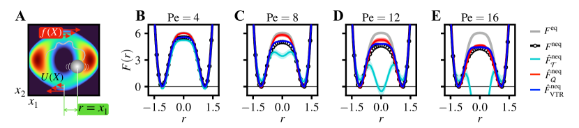
Figure 1: A. Two-dimensional Brownian particle in potential $U(X)$ undergoes linear shear, $f(X)$, at rate $\mathrm{Pe}$. B–E. Nonequilibrium free energy surfaces along order parameter $r=x_{1}$ (identified in panel A) at shear rates $\mathrm{Pe}=4,8,12,16$ evaluated with various estimators (lines), with the reference equilibrium free energy surface $F^{\mathrm{eq}}(r)$. The black circles evaluate the numerically exact nonequilibrium free energy surface $F^{\mathrm{neq}}(r)$ from histogram data at each shear rate.

Due to these considerations, we eschew online reinforcement learning of the optimal policy that saturates the supremum in Eq. (18) for general order parameters, in favor of a suboptimal but effective policy that can be estimated through offline regression on readily obtained NESS trajectory data; a similar approach has been used in related rare-event problems [56, 57]. In particular, we target the control policy that saturates the supremum in Eq. (18) for the identity order parameter such that $R(X)=X$, which takes the form

$$\varv^{\mathrm{neq}}(X)\,=\,f(X)-\beta^{-1}\nabla\ln\,\bm{[}\rho^{\mathrm{neq}}(X)/\rho^{\mathrm{eq}}(X)\bm{]}$$ (25)

and is derived in Appendix B. We recognize $\varv^{\mathrm{neq}}$ as the velocity field associated with the NESS configuration density $\rho^{\mathrm{neq}}$ through the steady-state Fokker–Planck equation

$$0\,=\,\bm{(}\mathscr{L}^{\dagger}\rho^{\mathrm{neq}}\bm{)}(X)\,=\,-\nabla\cdot\bm{(}\rho^{\mathrm{neq}}\,\varv^{\mathrm{neq}}\bm{)}(X)\;\forall\;X\in\Omega$$ (26)

with $\mathscr{L}^{\dagger}$ the $\mathrm{L}^{2}(\Omega)$-adjoint of the generator of the nonequilibrium dynamics governed by the SDE in Eq. (8) [33, ch. 4.1].

Control policy $\varv^{\mathrm{neq}}$ is generally suboptimal for order parameters that encode surjective (i.e., many-to-one) configuration mappings, failing to attain the supremum in Eq. (18) as follows from applying Jensen’s inequality. Indeed,

$$\lim_{T\to\infty} \ln\langle\exp\,\bm{[}\beta\mathcal{Q}_{T}(\bm{X})\bm{]}\rangle_{r}^{\mathrm{neq}}$$ (27)

$$\quad\geq\,{\textstyle\int_{\Omega}\mathrm{d}X\,\rho_{r}^{\mathrm{eq}}(X)}\lim_{T\to\infty}\ln\langle\exp\,\bm{[}\beta\mathcal{Q}_{T}(\bm{X})\bm{]}\rangle_{X}^{\mathrm{neq}}$$

$$\quad=\,{\textstyle\int_{\Omega}\mathrm{d}X\,\rho_{r}^{\mathrm{eq}}(X)}\lim_{T\to\infty}\sup_{\{\varv_{\bm{\theta}}\}}\,\langle\mathcal{R}_{T}(\bm{X},\bm{\theta})\rangle_{X}^{\varv_{\bm{\theta}}}$$

$$\quad\equiv\,\beta F^{\mathrm{eq}}(r)-\beta\hat{F}^{\mathrm{neq}}_{\mathrm{VTR}}(r)$$

with the inequality saturated only for invertible (i.e., one-to-one and onto) order parameters, and with the supremum attained at all $X\in\Omega$ up to an additive constant—stated in Appendix B—at the control policy $\varv_{\bm{\theta}}=\varv^{\mathrm{neq}}$ in Eq. (25). Despite this shortcoming, the central advantage of control policy $\varv^{\mathrm{neq}}$ is that it can be estimated without recourse to reinforcement learning methods, for instance by fitting NESS trajectory data through a steady-state velocity matching problem

$$\varv^{\mathrm{neq}}\,=\,\operatorname*{arg\,min}_{\{\varv_{\bm{\theta}}\}}\lim_{T\to\infty}\tfrac{1}{T}\Bigl{\langle}\textstyle\int_{0}^{T}\!\mathrm{d}t\,|\varv^{\mathrm{neq}}(X_{t})-\varv_{\bm{\theta}}(X_{t})|^{2}\Bigr{\rangle}^{\mathrm{neq}}$$ (28)

where $\varv_{\bm{\theta}}$ is a suitable policy ansatz.

In what follows, we work with ansätze $\varv_{\bm{\theta}}$ of the form

$$\varv_{\bm{\theta}}(X)\,=\,f(X)-\nabla V_{\bm{\theta}}(X)$$ (29)

where the control potential $V_{\bm{\theta}}$ is represented with a parametric differentiable ansatz. While a deep-learning solution to the steady-state velocity matching problem in Eq. (28) can most accurately estimate $\varv^{\mathrm{neq}}$ in complex applications [58, 18], our numerical tests show that simple, physically transparent parametrizations of the control potential $V_{\bm{\theta}}$ can yield substantial bias reduction in a variational estimate of the FES shift using the controlled estimator $\hat{F}^{\mathrm{neq}}_{\mathrm{VTR}}(r)$ introduced in Eq. (27), relative to perturbative estimates using $\hat{F}^{\mathrm{neq}}_{\mathcal{Q}}(r)$ in Eq. (16) and $\hat{F}^{\mathrm{neq}}_{\mathcal{T}}(r)$ in Eq. (17), at the minimal computational overhead of solving a linear system of equations corresponding to the velocity matching problem as detailed in Appendix C.

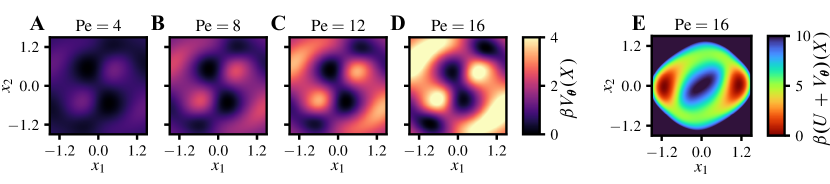
Figure 2: A–D. Optimized control potentials associated with the control policies used to evaluate $\hat{F}^{\mathrm{neq}}_{\mathrm{VTR}}(r)$ in Figs. 1B-E at the respective shear rates $\mathrm{Pe}$. E. The potential $U(X)+V_{\bm{\theta}}(X)$ at $\mathrm{Pe}=16$ yields the effective potential of a system whose equilibrium distribution encodes the NESS statistics of the sheared Brownian particle.

III Numerical illustrations

In this section, we discuss implementation details and illustrate the accuracy of estimators of $\beta F^{\mathrm{neq}}(r)$ introduced in the previous section, including the perturbative estimators $\beta\hat{F}^{\mathrm{neq}}_{\mathcal{Q}}(r)$ and $\beta\hat{F}^{\mathrm{neq}}_{\mathcal{T}}(r)$, and the variational time reversal estimator $\beta\hat{F}^{\mathrm{neq}}_{\mathrm{VTR}}(r)$. We consider a low-dimensional model where numerically exact results can be obtained, and a high-dimensional active filament where our methodology can lend insight into an activity driven collapse. We set $\beta=1$ and work with dimensionless units in both numerical examples.

III.1 Sheared particle in confined potential

As a simple model to compare nonequilibrium FES estimators, we consider the two-dimensional Brownian particle governed by nonequilibrium SDE in Eq. (8) with potential

$$U(X)\,=\,12+8x_{1}^{4}-12x_{2}^{2}+6x_{2}^{4}+20x_{1}^{2}(x_{2}^{2}-1)$$ (30)

and linear shear drift

$$f(X)\,=\,\mathrm{Pe}\;\bigl{(}\begin{smallmatrix}x_{2}\\ 0\end{smallmatrix}\bigr{)}$$ (31)

where $\mathrm{Pe}$ is the shear rate. This system is illustrated in Fig. 1A. At each $\mathrm{Pe}\!\neq\!0$, the particle evolves toward a nonequilibrium steady state with analytically unknown probability density $\rho^{\mathrm{neq}}(X)$. We characterize the associated nonequilibrium FES along the $x_{1}$ coordinate through estimators of the Kawasaki–Crooks relation in Eq. (13) introduced in Section II.

FES estimates were evaluated on a uniform grid along the order parameter coordinate comprised of $48$ equidistant points in the interval $[-1.95,1.95]$. At each grid point $r$, an ensemble of approximately $10^{4}$ particle configurations conditioned on $x_{1}\!=r$ was generated using an inverse transform sampler of the restricted equilibrium distribution with the density $\rho^{\mathrm{eq}}_{r}$ in Eq. (14); trapezoidal integration was used to estimate the equilibrium FES $F^{\mathrm{eq}}(r)$ directly from a histogram of the equilibrium probability density function. To estimate the nonequilibrium FES $F^{\mathrm{neq}}(r)$ at shear rates $\mathrm{Pe}\!\in\!\{4,8,12,16\}$ using the perturbative estimators in Eqs. (17), (16), and (27), at least $10^{4}$ configurations sampled from the conditional equilibrium ensemble at $r$ were evolved through numerical integration of SDEs (7), (8), and (19), respectively, over a long enough time interval to be distributed per the corresponding steady state. Whereas trajectories up to $80$ time units long were required to relax into the nonequilibrium steady states of the SDEs in Eqs. (8) and (19) across all order parameters values and shear rates, at least $300$ time units were needed for relaxation from each conditioned equilibrium ensemble into the unconditioned equilibrium ensemble through the equilibrium SDE in Eq. (7). The Euler–Maruyama method [59] was used to integrate all SDEs with a stepsize of $5\times 10^{-3}$ time units.

Deploying the estimators defined in Eqs. (16), (17), and (27) respectively yields the red, cyan, and blue free energy profiles in Figs. 1B-E. Also plotted is the empirically estimated nonequilibrium free energy surface, which is our ground truth for qualitative comparison with the perturbative and variational estimates. We find that the effect of an increasing shear rate $\mathrm{Pe}$ is to suppress the barrier height relative to the equilibrium free energy surface, while leaving the structure around the metastable points largely invariant. The traffic-based free energy estimator $\hat{F}^{\mathrm{neq}}_{\mathcal{T}}(r)$ is accurate at low $\mathrm{Pe}$ but rapidly deteriorates as $\mathrm{Pe}$ is increased. For $\mathrm{Pe}$ greater than $4$, this estimator erroneously predicts a metastable state at the top of the barrier, whose stability grows with increasing $\mathrm{Pe}$. Comparatively, the heat-based estimator $\hat{F}^{\mathrm{neq}}_{\mathcal{Q}}(r)$ shows better agreement with the ground truth barrier height across the range of shear rates considered, as well as the qualitative form of $\hat{F}^{\mathrm{neq}}(r)$. It is fortuitously accurate at the largest $\mathrm{Pe}$ considered, though less accurate at intermediate values.

The most accurate estimator with regards to barrier height is the variational estimator $\hat{F}^{\mathrm{neq}}_{\mathrm{VTR}}(r)$, though the estimate qualitatively deviates from the ground truth barrier shape at higher $\mathrm{Pe}$ due to the approximation error introduced by Jensen’s inequality in Eq. (27). The control potentials used to evaluate $\hat{F}^{\mathrm{neq}}_{\mathrm{VTR}}(r)$ are shown in Figs. 2A-D. Each potential was estimated by solving the velocity matching problem in Eq. (28) with the control policy ansatz in Eq. (29) and

$$\begin{gathered}V_{\bm{\theta}}(X)\,=\!\sum\limits_{i_{x_{1}}=\,0}^{N_{x_{1}}\!-1}\sum\limits_{i_{x_{2}}=\,0}^{N_{x_{2}}\!-1}\theta_{i_{x_{1}},i_{x_{2}}}\exp\,\bigl{(}-s^{2}|X-\mu_{i_{x_{1}},i_{x_{2}}}|^{2}/\>\!2\bigr{)}\\ \text{with}\;\;\mu_{i_{x_{1}},i_{x_{2}}}\!=\,\Delta\mu\,\Bigl{(}\begin{smallmatrix}i_{x_{1}}-(N_{x_{1}}-1)/2\\ i_{x_{2}}-(N_{x_{2}}-1)/2\end{smallmatrix}\Bigr{)}\,,\end{gathered}$$ (32)

where the parameter vector $\bm{\theta}\equiv(\theta_{i_{x_{1}},i_{x_{2}}})$ holds amplitude coefficients for squared-exponential functions with scale $s$ and locations $\bm{\{}\mu_{i_{x_{1}},i_{x_{2}}}\bm{\}}$ spanning a uniform grid on the $x_{1}x_{2}$-plane. For all $\mathrm{Pe}$, the control potential ansatz was instantiated using $256$ squared-exponential basis functions with scale parameter $s=0.25$ and locations spanning a $16\times 16$ origin-centered grid with spacing $\Delta\mu=0.25$ along the $x_{1}$ and $x_{2}$ coordinates. Optimal amplitude coefficients for the basis functions were obtained by solving for the parameter vector $\bm{\theta}$ at the global minimum of the functional in Eq. (28) through the system of equations derived for linear controller anzätze in Appendix C. At each shear rate, the steady-state averages used to solve for the optimal controller were estimated from $512$ independent steady-state realizations of Eq. (8) at least $25$ time units long.

The optimized control potentials in Figs. 2A-D show how particle configurations near the barrier top are stabilized by the nonequilibrium shear, thereby reducing the effective free energy barrier along the $x_{1}$ coordinate with increasing shear rate, as observed in Figs. 1B-E. Moreover, the sum of the equilibrium potential $U$ and the control potential $V_{\bm{\theta}}$, shown in Fig. 2E at $\mathrm{Pe}=16$, yields an effective equilibrium system with the correct nonequilibrium statistics of the sheared particle system, from which the nonequilibrium free energy surface in Fig. 1E can be recovered using equilibrium methods.

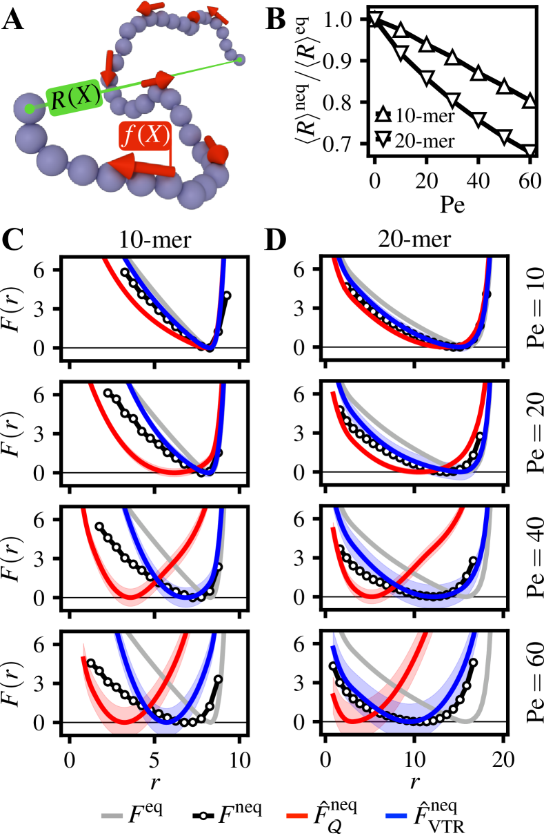
Figure 3: A. Schematic of a $20$-mer swimming filament featuring the nonequilibrium swimming force $f(X)$ and end-to-end distance $R(X)$ along the filament. B. Mean normalized end-to-end distance $\langle R\rangle^{\mathrm{neq}}/\langle R\rangle^{\mathrm{eq}}$ as a function of swimming speed $\mathrm{Pe}$ for $10$-mer and $20$-mer filaments. C, D. Free energy profiles along the end-to-end distance order parameter at various $\mathrm{Pe}$ using different estimators (lines) including the equilibrium free energy surface $F^{\mathrm{eq}}(r)$. The black circles estimate the nonequilibrium free energy surface $F^{\mathrm{neq}}(r)$ from histogram data at each $\mathrm{Pe}$.

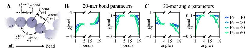
Figure 4: A. Schematic of parameters in the control policy ansatz, defined in Eq. (35). B, C. Dimensionless optimized values for control policy parameters for $20$-mer at various $\mathrm{Pe}$. Bond and angle parameter values close to the swimming filament’s termini are respectively shown in B and C.

III.2 Swimming filament

As a more challenging test of the nonequilibrium FES estimation methods introduced in Section II, we estimate the nonequilibrium FES along the end-to-end distance coordinate of the $N$-monomer swimming filament depicted in Fig. 3A. The filament’s dynamics is governed by the SDE in Eq. (8) with $U(X)$ a discretization of the potential energy of a self-excluding semiflexible Gaussian chain [60] and $f(X)$ a swimming force tangential to the filament. Representing the filament configuration as $X\!=\!(X^{(j)})_{j=1}^{N}$, with $X^{(j)}$ the position of the $j$th monomer along the chain, the potential energy is comprised by bond, bend, and WCA-type [61] exclusion interactions as

$$U(X)\,=\,U_{\mathrm{bond}}(X)\,+\,U_{\mathrm{bend}}(X)\,+\,U_{\mathrm{excl}}(X)$$ (33)

where

$$U_{\mathrm{bond}}(X) =\,\dfrac{k_{\mathrm{bond}}}{2} \textstyle\sum_{j=2}^{N}(|X^{(j)}-X^{(j-1)}|-\ell_{\mathrm{bond}})^{2}$$

$$U_{\mathrm{bend}}(X) =\,\dfrac{k_{\mathrm{bend}}}{2} \textstyle\sum_{j=3}^{N}|X^{(j)}-2X^{(j-1)}+X^{(j-2)}|^{2}$$

$$U_{\mathrm{excl}}(X) =\,2\varepsilon_{\mathrm{excl}} \textstyle\sum_{\begin{subarray}{c}j\neq k=1\end{subarray}}^{N}\bm{\biggl{[}}\dfrac{1}{4}+\biggl{(}\dfrac{\sigma_{\mathrm{excl}}}{d_{j,k}}\biggr{)}^{\!12}-\biggl{(}\dfrac{\sigma_{\mathrm{excl}}}{d_{j,k}}\biggr{)}^{\!6}\,\bm{\biggr{]}}$$

with $d_{j,k}=\min(|X^{(j)}-X^{(k)}|,\,2^{1/6}\sigma^{\mathrm{excl}})$. We work with units such that $\varepsilon_{\mathrm{excl}}\equiv 1$ and $\sigma_{\mathrm{excl}}\equiv 1$ and set $k_{\mathrm{bond}}=1000(\beta\sigma_{\mathrm{excl}}^{2})^{-1}$, $k_{\mathrm{bend}}=10(\beta\sigma_{\mathrm{excl}}^{2})^{-1}$, and $\ell_{\mathrm{bond}}=2^{1/6}\sigma_{\mathrm{excl}}$. The filament swims along its contour at speed $\mathrm{Pe}$, advected with the nonequilibrium drift $f(X)=\bm{(}f^{(j)}(X)\bm{)}_{j=1}^{N}$ where

$$f^{(j)}(X)\,=\,\dfrac{\mathrm{Pe}}{2}\times\begin{cases}U_{j,j+1}&j=1\\ U_{j,j+1}+U_{j-1,j}&j=2,\!...,N\!-1\\ U_{j,j-1}&j=N\\ \end{cases}$$ (34)

is the swimming force on the $j$th monomer, defined in terms of $U_{j,k}\!=\!(X^{(k)}-X^{(j)})/|X^{(k)}-X^{(j)}|$ the unit vector parallel to the displacement between monomers $j$ and $k$.

The phenomenology of the swimming filament has been explored across a broad range of monomer numbers $N$ in earlier work [62, 63], and is illustrated for $10$-mer and $20$-mer filaments in Fig. 3B. Notably, the steady-state mean end-to-end distance $R(X)=|X^{(N)}-X^{(1)}|$ monotonically decreases with increasing swimming speed, since the head of the swimming filament swerves more frequently at higher swimming speeds. This swerve of the head, which moves more slowly then the body of the filament, then results in a buckling of filament configurations. These buckling motions become more typical as the system is driven away from equilibrium. Further, larger chains have large propulsive forces, as they are additive along the chain, resulting in higher likelihood of buckling and a more pronounced decrease of end-to-end distance with $\mathrm{Pe}$.

To estimate FESs along the end-to-end distance coordinate, $r$-conditioned equilibrium ensembles were approximated with umbrella-biased equilibrium ensembles per

$$\rho^{\mathrm{eq}}_{r}(X)\,\approx\,\rho^{\mathrm{eq}}(X)\,\dfrac{\exp\,\bm{[}-\beta U^{\mathrm{umb}}\bm{(}R(X)\bm{)}\bm{]}}{\textstyle\int_{\Omega}\mathrm{d}X^{\prime}\,\exp\,\bm{[}-\beta U^{\mathrm{umb}}\bm{(}R(X^{\prime})\bm{)}\bm{]}}$$

where the umbrella potentials

$$U^{\mathrm{umb}}(r)\,=\,k^{\mathrm{umb}}(r-\ell^{\mathrm{umb}})^{2}/\>\!2$$

were assigned stiffness $k^{\mathrm{umb}}=100(\beta\sigma_{\mathrm{excl}}^{2})^{-1}$ and locations $\ell^{\mathrm{umb}}$ spanning a uniform grid along the end-to-end distance coordinate, with values in the interval $\bm{(}0,(N-1)\ell^{\mathrm{bond}}\bm{)}$ for each $N$-mer. The WHAM procedure [64, 65] was used to estimate the equilibrium FES $F^{\mathrm{eq}}(r)$ from the array of umbrella-biased ensembles. Separately, a reference estimate of the nonequilibrium FES $F^{\mathrm{neq}}(r)$ at swimming speeds $\mathrm{Pe}\in\{10,20,40,60\}$ was obtained from a histogram of the end-to-end distance along a steady-state realization of (8) integrated out to $10^{3}$ time units using the Euler–Maruyama method with stepsizes as small as $10^{-5}$ for numerical stability. Nonequilibrium FES estimates $\hat{F}^{\mathrm{neq}}_{\mathcal{Q}}(r)$ and $\hat{F}^{\mathrm{neq}}_{\mathrm{VTR}}(r)$ were evaluated by integrating $10^{5}$ relaxation trajectories using the SDEs in Eqs. (8) and (19), respectively, with the order parameter value $r$ of each estimate given by the mean end-to-end distance of the approximately conditioned ensemble in which relaxation trajectories were initialized. All relaxation trajectory ensembles were integrated out to $25$ time units using the Euler–Maruyama method at stepsizes as small as $10^{-6}$ time units to ensure numerical stability.

FES estimates from steady-state trajectory histogramming and variational estimators are shown for $10$-mer and $20$-mer filaments in Fig. 3C and Fig. 3D for swimming speeds ranging between $\mathrm{Pe}=10$ and $\mathrm{Pe}=60$ units. The equilibrium free energy surface for each $N$-mer is also shown in its respective panels. Across all $\mathrm{Pe}$ values for the $10$-mer and $20$-mer filaments, we find better qualitative agreement between the brute-force nonequilibrium free energy and the variational estimator $\hat{F}^{\mathrm{neq}}_{\mathrm{VTR}}(r)$ than the perturbative $\hat{F}^{\mathrm{neq}}_{\mathcal{Q}}(r)$, though both estimators exhibit notable bias at higher $\mathrm{Pe}$ values. Both estimators correctly predict a collapse of the filament with increasing $\mathrm{Pe}$, though $\hat{F}^{\mathrm{neq}}_{\mathcal{Q}}(r)$ underestimates the value of the $\mathrm{Pe}$ where this occurs, as evident in the movement of the minimum in $F^{\mathrm{neq}}(r)$ to small values of $r$ with increasing $\mathrm{Pe}$. The variational estimator accurately predicts the behavior of $F^{\mathrm{neq}}(r)$ near its typical values across the range of $\mathrm{Pe}$ for both chains, though exhibits deviations from the ground truth away from the typical value for the 10-mer. The traffic-based perturbative estimator $\hat{F}^{\mathrm{neq}}_{\mathcal{T}}(r)$ is sufficiently inaccurate for all $\mathrm{Pe}$ as to be remotely outside the range in Figs. 3C-D, and is hence omitted in the current discussion.

Figure 4A illustrates the interactions that comprise the control potential used to evaluate the nonequilibrium FES estimator $\hat{F}^{\mathrm{neq}}_{\mathrm{VTR}}(r)$. Control potential terms are similar to the bond and bend interactions in the potential energy function in Eq. (33), but have individual stiffness and scale parameters for each bond and bend interaction along the filament. The control potential entering $\varv_{\bm{\theta}}$ is

$$V_{\bm{\theta}}(X)=\,\textstyle\sum_{j=2}^{N}k_{j}^{\mathrm{bond}}(|X^{(j)}-X^{(j-1)}|-\ell_{j}^{\mathrm{bond}})^{2}/\>\!2$$ (35)

$$\;\,+\,\textstyle\sum_{j=3}^{N}k_{j}^{\mathrm{bend}}(|X^{(j)}-2X^{(j-1)}+X^{(j-2)}|-\ell_{j}^{\mathrm{bend}})^{2}/\>\!2$$

where $\bm{\theta}\equiv\{(k_{j}^{\mathrm{bond}},\ell_{j}^{\mathrm{bond}})_{j=2}^{N},(k_{j}^{\mathrm{bend}},\ell_{j}^{\mathrm{bend}})_{j=3}^{N}\}$ is the policy parameter vector. Control potential parameter values were optimized at each swimming speed $\mathrm{Pe}\!\in\!\{10,20,40,60\}$ and each monomer number $N\!\in\!\{10,20\}$ via stochastic gradient descent of the loss function in Eq. (46) in Appendix C, using $128$ independent steady-state realizations of the nonequilibrium SDE in Eq. (8) at least $25$ time units long, and learning rates up to $10^{-1}$. Optimized control potential parameters for a swimming $20$-mer at speeds ranging from $\mathrm{Pe}=10$ to $\mathrm{Pe}=60$ units are shown in Fig. 4B and Fig. 4C, which respectively show bond and bend interaction parameters near the swimming filament’s endpoints. Viewed as a correction to the filament’s potential energy function, the optimized control potential shifts internal tensions within the swimming filament to stabilize typical structural bond and bend deformations near the filament’s tail ($1$st) and head ($N$th) monomers in the NESS. The localization of the optimized control potential to the boundaries of the chain explains the higher accuracy of the results for the $20$-mer compared to the $10$-mer in Figs. 3C-D. For longer chains, the potential contribution of the control policy plays a smaller role than the reversing of the active force, and so comparable errors in the estimate of the optimal control in the larger chain result in small biases to the free energy surface.

IV Conclusions

Growing interest in the physics of driven and active matter demands rapid progress toward turnkey simulation methods for the thermodynamic modeling of structure and stability of systems driven far from equilibrium. Building from a natural generalization of the thermodynamic free energy surface to nonequilibrium systems, the current work adopts an optimal control viewpoint of a key result in stochastic thermodynamics—the Kawasaki–Crooks relation—to offer a free-energy surface estimation scheme for nonequilibrium steady states governed by overdamped Langevin dynamics. Illustrative applications of the method to active matter models show that approximately optimally controlled nonequilibrium free energy estimators can exhibit reduced bias relative to the perturbative approaches at the state of the art. The control-based free energy estimator does require optimizing a control policy ansätze in each application, but as shown above, simple policy parametrizations can be optimized with little computational overhead and in an offline manner through regression from steady-state trajectory data.

Our formal approach in this work highlights deep connections between the fluctuation theorems at the heart of stochastic thermodynamics and the formalism of stochastic control theory [66, 67, 68, 69, 70], paving the way to migrate generative modeling tools based on variational time reversal of diffusive processes [71, 72, 73] into chemical and biological physics for nonequilibrium structure and stability quantification.

All numerical results presented in this work, along with generating code, are deposited in the GitHub repository jrosaraices/nonequilibrium-vtr.

Appendix A Derivation of the Kawasaki–Crooks relation for nonequilibrium free energy shifts

In this section, we derive the Kawasaki–Crooks equality in Eq. (13), relating the free energy surface shift in Eq. (6) to an average over nonequilibrium trajectories initialized at order parameter value $r$. To this end, we consider the Dirac observable $\delta\bm{(}R(X_{T})-r\bm{)}$ that yields the time-dependent nonequilibrium likelihood at $r$ through the relation $P_{T}(r)=\langle\delta\bm{(}R(X_{T})-r\bm{)}\rangle^{\mathrm{neq}}$, where the superscript on the angled brackets denotes expectation with respect to the path probability measure induced by the SDE in Eq. (8) with equilibrium initial conditions. This expectation may be manipulated as follows:

$$P_{T}(r)\, =\,\langle\delta\bm{(}R(X_{T})-r\bm{)}\rangle^{\mathrm{neq}}$$ (36a)

$$=\,\langle\exp\,\bm{[}-\beta\mathcal{S}_{T}(\bm{X})\bm{]}\,\delta\bm{(}R(X_{T})-r\bm{)}\rangle^{\mathrm{eq}}$$ (36b)

$$=\,\langle\exp\,\bm{[}-\beta\mathcal{S}_{T}(\tilde{\bm{X}})\bm{]}\,\delta\bm{(}R(X_{0})-r\bm{)}\rangle^{\mathrm{eq}}$$ (36c)

$$=\,\langle\exp\,\bm{[}-\beta\mathcal{S}_{T}(\tilde{\bm{X}})\bm{]}\rangle_{r}^{\mathrm{eq}}\,P_{0}(r)$$ (36d)

$$=\,\langle\exp\,\bm{[}-\beta(\mathcal{S}_{T}-\mathcal{Q}_{T})(\bm{X})\bm{]}\rangle_{r}^{\mathrm{eq}}\,P_{0}(r)$$ (36e)

$$=\,\langle\exp\,\bm{[}\beta\mathcal{Q}_{T}(\bm{X})\bm{]}\rangle_{r}^{\mathrm{neq}}\,P_{0}(r)$$ (36f)

In Eq. (36b), the path expectation in Eq. (36a) is rewritten in terms of an equilibrium path ensemble generated by the SDE in Eq. (7) initialized at equilibrium, with the pathwise change of measure given by Eq. (9). Invariance under time reversal of the equilibrium path ensemble allows shifting the Dirac observable across the time interval via pathwise time involution, which yields Eq. (36c). Then, the Markov property allows introducing the conditional expectation in Eq. (36d), which averages over paths initialized per the restricted equilibrium density in Eq. (14). Finally, Eq. (12) is used to write the change of measure in terms of the excess heat in Eq. (36e), and the remainder is absorbed into the path measure to reintroduce the nonequilibrium path ensemble in Eq. (36f).

From Eq. (36), the nonequilibrium free energy shift in the long-time limit takes the form

$$\ln\dfrac{P^{\mathrm{neq}}(r)}{P^{\mathrm{eq}}(r)} =\,\lim_{T\to\infty}\ln\dfrac{P_{T}(r)}{P_{0}(r)}$$ (37)

$$=\,\lim_{T\to\infty}\ln{\langle\exp\,\bm{[}\beta\mathcal{Q}_{T}(\bm{X})\bm{]}\rangle^{\mathrm{neq}}_{r}}$$

which corresponds to the sought-after result.

The Kawasaki–Crooks equality in Eq. (13) is related to the integral fluctuation relation in Eq. (15) for the excess heat $\mathcal{Q}_{T}$. This is a consequence of the fact that

$$\langle\exp\,\bm{[}\beta\mathcal{Q}_{T}(\bm{X})\bm{]}\rangle^{\mathrm{neq}}\, =\,\langle\exp\,\bm{[}-\beta(\mathcal{S}_{T}-\mathcal{Q}_{T})(\bm{X})\bm{]}\rangle^{\mathrm{eq}}$$ (38a)

$$=\,\langle\exp\,\bm{[}-\beta\mathcal{S}_{T}(\tilde{\bm{X}})\bm{]}\rangle^{\mathrm{eq}}$$ (38b)

$$=\,\langle\exp\,\bm{[}-\beta\mathcal{S}_{T}(\bm{X})\bm{]}\rangle^{\mathrm{eq}}$$ (38c)

$$=\,\langle 1\rangle^{\mathrm{neq}}=1$$ (38d)

where Eq. (38c) used the fact that the path ensemble generated by the equilibrium SDE in Eq. (7) with equilibrium initial conditions is invariant under time reversal.

Appendix B Derivation and evaluation of optimal control policy for the configuration-wise Kawasaki–Crooks equality

For the identity order parameter such that $R(X)=X$ specifies an initial configuration (rather than an equilibrium ensemble of configurations with a given conformation $r$), the general Kawasaki–Crooks equality in Eq. (13) reduces to the configuration-wise form

$$\dfrac{\rho^{\mathrm{neq}}(X)}{\rho^{\mathrm{eq}}(X)}\,=\,\lim_{T\to\infty}\langle\exp\,\bm{[}\beta\mathcal{Q}_{T}(\bm{X})\bm{]}\rangle_{X}^{\mathrm{neq}}\,\equiv\,\exp\bm{(}V(X)\bm{)}$$ (39)

Applying the Feynman–Kaç theorem [74, thm. 10.2] to the exponential average reveals that $\exp(V)$ solves the steady-state backward Kolmogorov equation

$$0\,=\,-\bm{[}\mathscr{L}-2f\cdot\nabla+\beta\nabla U\cdot f\bm{]}\exp(V)$$ (40)

where $\mathscr{L}$ is the generator of the nonequilibrium trajectory ensemble governed by the SDE in Eq. (8), namely

$$\mathscr{L}\,=\,(f-\nabla U)\cdot\nabla+\beta^{-1}\Delta$$ (41)

The tilted generator in Eq. (40) is associated with a non measure-preserving stochastic dynamics and would suggest that Eq. (39) must be estimated in simulation through population dynamics approaches that, despite recent improvements [75, 42, 76, 77], remain notorious for their high statistical variance in the relevant long-time limit [77, 78]. Fortunately, the generalized Doob transform [79, Section IV] of the tilted generator yields a statistically equivalent, yet measure-preserving, stochastic dynamics that allows variational, minimal-variance estimation of the exponential averages in Eq. (39).

To compute the generalized Doob transform, observe that the tilted generator satisfies the operator equality

$$\mathscr{L}-2f\cdot\nabla+\beta\nabla U\cdot f\,=\,(\rho^{\mathrm{eq}})^{-1}\circ\mathscr{L}^{\dagger}\circ\rho^{\mathrm{eq}}$$ (42)

with $\mathscr{L}^{\dagger}$ the Fokker–Planck operator introduced in Eq. (26). Indeed, for any suitably differentiable scalar function $g$,

$$\bm{[}(\rho^{\mathrm{eq}})^{-1}\circ\mathscr{L}^{\dagger}\circ\rho^{\mathrm{eq}}\bm{]}\,g$$

$$\;=\,(\rho^{\mathrm{eq}})^{-1}\bm{\{}-\nabla\cdot\bm{[}(f-\nabla U)\,\rho^{\mathrm{eq}}g\bm{]}+\beta^{-1}\Delta(\rho^{\mathrm{eq}}g)\bm{\}}$$

$$\;=\,(-f-\nabla U)\cdot\nabla g+\beta^{-1}\Delta g+\beta g\,\nabla U\cdot f$$

$$\;=\,\bm{[}\mathscr{L}-2f\cdot\nabla+\beta\nabla U\cdot f\bm{]}\,g$$

With this, using Eq. (39) we find that the Doob-transformed tilted generator is

$$\exp(-V)\circ\bm{[}(\rho^{\mathrm{eq}})^{-1}\circ\mathscr{L}^{\dagger}\circ\rho^{\mathrm{eq}}\bm{]}\circ\exp(V)$$ (43)

$$\quad=\,(\rho^{\mathrm{ne}})^{-1}\circ\mathscr{L}^{\dagger}\circ\rho^{\mathrm{ne}}\,=\,\mathscr{L}-2(f-\beta^{-1}\nabla V)\cdot\nabla$$

which corresponds to the controlled SDE in Eq. (19) with the control policy $\varv^{\mathrm{neq}}$ in Eq. (25). To see that this controlled dynamics indeed yields a minimum-variance, variational estimate of Eq. (39), note that for every realization $\bm{X}$ of the nonequilibrium SDE in Eq. (19) initialized at the configuration $X$, the logarithm of the expectand in the second line of Eq. (18) reduces to

$$\beta\mathcal{Q}_{T}(\bm{X})+\ln\dfrac{\mathrm{d}\mathbb{P}^{\mathrm{neq}}(\bm{X})}{\mathrm{d}\mathbb{P}^{\varv^{\mathrm{neq}}}(\bm{X})}\, =\,\beta\mathcal{Q}_{T}(\bm{X})-\beta\textstyle\int_{0}^{T}\!\mathrm{d}t\,|\varv^{\mathrm{neq}}(X_{t})|^{2}+\sqrt{2\beta}\textstyle\int_{0}^{T}\mathrm{d}W_{t}\cdot\varv^{\mathrm{neq}}(X_{t})$$ (44a)

$$=\,\beta\mathcal{Q}_{T}(\bm{X})+\beta\textstyle\int_{0}^{T}\!\mathrm{d}t\,\bm{\{}|\varv^{\mathrm{neq}}(X_{t})|^{2}+\bm{[}(\beta^{-1}\nabla+f-\nabla U)\cdot\varv^{\mathrm{neq}}\bm{]}(X_{t})\bm{\}}-\mathrm{d}X_{t}\circ\varv^{\mathrm{neq}}(X_{t})$$ (44b)

$$=\,\textstyle\int_{0}^{T}\!\mathrm{d}t\,\bm{[}\beta^{-1}(|\nabla V|^{2}+\Delta V)-(f+\nabla U)\cdot\nabla V+\beta\nabla U\cdot f\bm{]}(X_{t})-\mathrm{d}X_{t}\circ\nabla V(X_{t})$$ (44c)

$$=\,\textstyle\int_{0}^{T}\!\mathrm{d}t\exp\bm{(}-V(X_{t})\bm{)}\,\bm{[}\mathscr{L}-2f\cdot\nabla+\beta\nabla U\cdot f\bm{]}\exp\bm{(}V(X_{t})\bm{)}-\mathrm{d}X_{t}\circ\nabla V(X_{t})$$ (44d)

$$=\,-\textstyle\int_{0}^{T}\mathrm{d}X_{t}\circ\nabla V(X_{t})\,=\,V(X)-V(X_{T})$$ (44e)

where Itō’s formula [33, ch. 3.4] obtains Eq. (44b), the heat functional vanished due to cancellation in Eq. (44c), the Hopf–Cole substitution $V\!\to\exp(V)$ leads to Eq. (44d), and Eq. (40) finally yields the potential difference Eq. (44e). Averaging this difference against realizations of the optimally controlled SDE in Eq. (19) yields a remarkably simple lower bound on the configuration-wise Kawasaki–Crooks equality in Eq. (39):

$$\ln\dfrac{\rho^{\mathrm{neq}}(X)}{\rho^{\mathrm{eq}}(X)} \geq\,\lim_{T\to\infty}\Bigl{\langle}\beta\mathcal{Q}_{T}(\bm{X})+\ln\dfrac{\mathrm{d}\mathbb{P}^{\mathrm{neq}}(\bm{X})}{\mathrm{d}\mathbb{P}^{\varv^{\mathrm{neq}}}(\bm{X})}\Bigr{\rangle}_{X}^{\varv^{\mathrm{neq}}}$$ (45)

$$=\,V(X)-\lim_{T\to\infty}\langle V(X_{T})\rangle_{X}^{\varv^{\mathrm{neq}}}$$

$$=\,\ln\dfrac{\rho^{\mathrm{neq}}(X)}{\rho^{\mathrm{eq}}(X)}-\mathcal{D}_{\mathrm{KL}}(\rho^{\mathrm{neq}}\|\rho^{\mathrm{eq}})$$

This lower bound on Eq. (39) is free of trajectory functionals associated with time-extensive statistical variance, instead stating a trivial inequality involving the nonnegative excess free energy of the NESS in Eq. (4). The Kullback–Leibler divergence in the last equality appears because the controlled SDE in Eq. (19), when equipped with the control policy $\varv^{\bm{\theta}}=\varv^{\mathrm{neq}}$ given in Eq. (25), has the same invariant distribution as the SDE in Eq. (8). This follows from the fact that the $\mathrm{L}^{2}(\Omega)$-adjoint of the controlled generator in Eq. (43) also satisfies the steady-state Fokker–Planck equation in Eq. (26). Hence, an unbiased estimate of the Kullback–Leibler divergence in Eq. (45) can be obtained from a time average of the optimal control potential $V$ over a long realization of either the nonequilibrium SDE in Eq. (8) or the controlled SDE in Eq. (19) with control policy $\varv^{\bm{\theta}}=\varv^{\mathrm{neq}}$.

Appendix C Derivation of linear solution to velocity matching problem

As discussed in Section II.3 of the main text, the optimal control policy in Eq. (25) must be estimated to evaluate the Kawasaki–Crooks estimator $\hat{F}^{\mathrm{neq}}_{\mathrm{VTR}}(r)$ in Eq. (27). This entails minimizing the mean-squared error function in Eq. (28), namely

$$\lim_{T\to\infty}\tfrac{1}{T}\Bigl{\langle}\textstyle\int_{0}^{T}\!\mathrm{d}t\,|\varv^{\mathrm{neq}}(X_{t})-\varv_{\bm{\theta}}(X_{t})|^{2}\Bigr{\rangle}^{\mathrm{neq}}$$

with respect to policy ansatz parameters $\bm{\theta}$. Expanding the square inside the expectation produces linear and quadratic terms in the unknown target policy $\varv^{\mathrm{neq}}$, which must be eliminated for actual computation. The quadratic term can simply be dropped, and for the linear term we observe that for any suitably differentiable vector function $h$,

$$\Bigl{\langle} \textstyle\int_{0}^{T}\!\mathrm{d}t\,h(X_{t})\cdot\varv^{\mathrm{neq}}(X_{t})\Bigr{\rangle}^{\mathrm{neq}}$$

$$=\Bigl{\langle}\textstyle\int_{0}^{T}\!\mathrm{d}t\,h(X_{t})\cdot(f-\nabla U-\beta^{-1}\nabla\ln\rho^{\mathrm{neq}})(X_{t})\Bigr{\rangle}^{\mathrm{neq}}$$

$$=\Bigl{\langle}\textstyle\int_{0}^{T}h(X_{t})\cdot\bm{[}(f-\nabla U)(X_{t})\,\mathrm{d}t+\sqrt{2\smash[t]{\beta^{-1}}}\,\mathrm{d}W_{t}\bm{]}\Bigr{\rangle}^{\mathrm{neq}}$$

$$\phantom{=}-\beta^{-1}\textstyle\int_{0}^{T}\mathrm{d}t\textstyle\int_{\Omega}\mathrm{d}X\,\rho^{\mathrm{neq}}(X)\bm{[}h(X)\cdot\nabla\ln\rho^{\mathrm{neq}}(X)\bm{]}$$

$$=\Bigl{\langle}\textstyle\int_{0}^{T}h(X_{t})\cdot\mathrm{d}X_{t}\Bigr{\rangle}^{\mathrm{neq}}$$

$$\phantom{=}+\beta^{-1}\textstyle\int_{0}^{T}\mathrm{d}t\textstyle\int_{\Omega}\mathrm{d}X\,\rho^{\mathrm{neq}}(X)\bm{(}\nabla\cdot h\bm{)}(X)$$

$$=\Bigl{\langle}\textstyle\int_{0}^{T}h(X_{t})\circ\mathrm{d}X_{t}\Bigr{\rangle}^{\mathrm{neq}}$$

where we used Eq. (25) in the first equality, Eq. (8) in the second equality, integration by parts in the third equality, and the definition of the Stratonovich integral in the fourth equality. Fully eliminating the target velocity from the mean squared error yields the loss function

$$\mathsf{L}(\bm{\theta})\,=\,\lim_{T\to\infty}\tfrac{1}{T}\Bigl{\langle}\textstyle\int_{0}^{T}|\varv_{\bm{\theta}}(X_{t})|^{2}\,\mathrm{d}t-2\varv_{\bm{\theta}}(X_{t})\circ\mathrm{d}X_{t}\Bigr{\rangle}^{\mathrm{neq}}$$ (46)

to be minimized with respect to variations in the policy parameters $\bm{\theta}$. Using the control policy ansatz $\varv_{\bm{\theta}}$ in Eq. (29) leaves only the control potential $V_{\bm{\theta}}$ up to parametric estimation. The gradient of the loss function in Eq. (46) with respect to policy parameters $\bm{\theta}$ may be written in terms of control potential derivatives as

$$\nabla_{\bm{\theta}}\mathsf{L}(\bm{\theta}) \,=\,\lim_{T\to\infty}\tfrac{1}{T}\Bigl{\langle}\textstyle\int_{0}^{T}\mathrm{d}t\,\nabla_{\bm{\theta}}\,\bm{[}|\varv_{\bm{\theta}}(X_{t})|^{2}$$

$$\qquad\qquad\quad-2\,\mathrm{d}X_{t}\circ\varv_{\bm{\theta}}(X_{t})\bm{]}\Bigr{\rangle}^{\mathrm{neq}}$$

$$\,=\,\lim_{T\to\infty}\tfrac{2}{T}\Bigl{\langle}\textstyle\int_{0}^{T}\mathrm{d}t\,(\nabla V_{\bm{\theta}}-f)(X_{t})\cdot\nabla_{\bm{\theta}}\nabla V_{\bm{\theta}}(X_{t})$$

$$\qquad\qquad\quad+\mathrm{d}X_{t}\circ\nabla_{\bm{\theta}}\nabla V_{\bm{\theta}}(X_{t})\Bigr{\rangle}^{\mathrm{neq}}$$

A linear representation of the control potential such as

$$V_{\bm{\theta}}(X)\,=\,\textstyle\sum_{i}\bm{\theta}_{i}\phi_{i}(X)$$ (47)

where $\bm{\{}\phi_{i}(\cdot)\bm{\}}$ is a basis of suitably differentiable scalar functions, leads to the following system of equations for $\bm{\theta}$ at the global minimum of Eq. (46) and the original loss functional in Eq. (28):

$$0\,=\,\lim_{T\to\infty}\tfrac{1}{T}\Bigl{\langle} \textstyle\int_{0}^{T}\mathrm{d}t\,\bm{\bigl{[}}\textstyle\sum_{j}\theta_{j}(\nabla\phi_{j}-f)(X_{t})\bm{\bigr{]}}\cdot\nabla\phi_{i}(X_{t})$$ (48)

$$+\,\textstyle\int_{0}^{T}\mathrm{d}X_{t}\circ\nabla\phi_{i}(X_{t})\Bigr{\rangle}^{\mathrm{neq}}\quad\forall\;i$$

Building this linear system merely requires the evaluation of steady-state averages of scalar products of the differentiated basis $\bm{\{}\nabla\phi_{i}(\cdot)\bm{\}}$. In detail, Eq. (48) may be rewritten as

$$0\,=\,\textstyle\sum_{j}\theta_{j}\mathsf{A}_{ij}\,-\,\mathsf{b}_{i}\,+\,\mathsf{c}_{i}\quad\forall\;i$$

where

$$\mathsf{A}_{ij} =\,\lim_{T\to\infty}\tfrac{1}{T}\Bigl{\langle}\textstyle\int_{0}^{T}\mathrm{d}t\,\nabla\phi_{i}(X_{t})\cdot\nabla\phi_{j}(X_{t})\Bigr{\rangle}^{\mathrm{neq}}$$

$$\mathsf{b}_{i} =\,\lim_{T\to\infty}\tfrac{1}{T}\Bigl{\langle}\textstyle\int_{0}^{T}\mathrm{d}t\,\nabla\phi_{i}(X_{t})\cdot f(X_{t})\Bigr{\rangle}^{\mathrm{neq}}$$

$$\mathsf{c}_{i} =\,\lim_{T\to\infty}\tfrac{1}{T}\Bigl{\langle}\textstyle\int_{0}^{T}\mathrm{d}X_{t}\circ\nabla\phi_{i}(X_{t})\Bigr{\rangle}^{\mathrm{neq}}$$

with $i,\,j$ indexing the control potential basis.

References

- Muegge and Hu [2023] I. Muegge and Y. Hu, ACS Medicinal Chemistry Letters 14, 244 (2023).
- Cournia et al. [2021] Z. Cournia, C. Chipot, B. Roux, D. M. York, and W. Sherman, in Free energy methods in drug discovery: Current state and future directions, edited by K. A. Armacost and D. C. Thompson (American Chemical Society, 2021), chap. 1.
- Mobley and Klimovich [2012] D. L. Mobley and P. V. Klimovich, The Journal of Chemical Physics 137, 230901 (2012).
- Lee et al. [2021] S. Lee, B. Kim, H. Cho, H. Lee, S. Y. Lee, E. S. Cho, and J. Kim, ACS Applied Materials & Interfaces 13, 23647 (2021).
- Kim et al. [2012] J. Kim, L.-C. Lin, R. L. Martin, J. A. Swisher, M. Haranczyk, and B. Smit, Langmuir 28, 11914 (2012).
- Rickman and LeSar [2002] J. M. Rickman and R. LeSar, Annual Review of Materials Research 32, 195 (2002).
- Chipot [2023] C. Chipot, Annual Review of Biophysics 52, 113 (2023).
- Axelrod et al. [2022] S. Axelrod, D. Schwalbe-Koda, S. Mohapatra, J. Damewood, K. P. Greenman, and R. Gómez-Bombarelli, Accounts of Materials Research 3, 343 (2022).
- York [2023] D. M. York, ACS Physical Chemistry Au 3, 478 (2023).
- Dickson and Dinner [2010] A. Dickson and A. R. Dinner, Annual Review of Physical Chemistry 61, 441 (2010).
- Allen et al. [2009] R. J. Allen, C. Valeriani, and P. R. ten Wolde, Journal of Physics: Condensed Matter 21, 463102 (2009).
- Zuckerman and Chong [2017] D. M. Zuckerman and L. T. Chong, Annual Review of Biophysics 46, 43 (2017).
- Hall et al. [2022] S. W. Hall, G. Díaz Leines, S. Sarupria, and J. Rogal, The Journal of Chemical Physics 156, 200901 (2022).
- Seifert [2012] U. Seifert, Reports on Progress in Physics 75, 126001 (2012).
- Crooks [2001] G. E. Crooks, PhD thesis, University of California, Berkeley (2001).
- Das and Limmer [2019] A. Das and D. T. Limmer, The Journal of Chemical Physics 151, 244123 (2019).
- Das et al. [2021] A. Das, D. C. Rose, J. P. Garrahan, and D. T. Limmer, The Journal of Chemical Physics 155, 134105 (2021).
- Boffi and Vanden-Eijnden [2023a] N. M. Boffi and E. Vanden-Eijnden, Deep learning probability flows and entropy production rates in active matter (2023a), eprint arXiv:2309.12991.
- Gibbs [1928] J. W. Gibbs, The collected works of J. Willard Gibbs: Thermodynamics, vol. 1 (Longmans, Green and Company, 1928).
- Gaveau et al. [2002] B. Gaveau, K. Martinás, M. Moreau, and J. Tóth, Physica A: Statistical Mechanics and its Applications 305, 445 (2002).
- Sivak and Crooks [2012] D. A. Sivak and G. E. Crooks, Physical Review Letters 108, 150601 (2012).
- Kirkwood [1935] J. G. Kirkwood, The Journal of Chemical Physics 3, 300 (1935).
- Zwanzig [2001] R. Zwanzig, Nonequilibrium statistical mechanics (Oxford University Press, 2001), 1st ed.
- Baiesi and Maes [2013] M. Baiesi and C. Maes, New Journal of Physics 15, 013004 (2013).
- Torrie and Valleau [1977] G. M. Torrie and J. P. Valleau, Journal of Computational Physics 23, 187 (1977).
- Laio and Gervasio [2008] A. Laio and F. L. Gervasio, Reports on Progress in Physics 71, 126601 (2008).
- Comer et al. [2015] J. Comer, J. C. Gumbart, J. Hénin, T. Lelièvre, A. Pohorille, and C. Chipot, The Journal of Physical Chemistry B 119, 1129 (2015).
- Lelièvre et al. [2010] T. Lelièvre, M. Rousset, and G. Stoltz, Free energy computations: A mathematical perspective (Imperial College Press, 2010), 1st ed.
- Frenkel and Smit [2023] D. Frenkel and B. Smit, Understanding molecular simulation: From algorithms to applications (Academic Press, Inc., 2023), 3rd ed.
- Risken [1996] H. Risken, The Fokker–Planck equation: Methods of solution and applications (Springer Berlin, Heidelberg, 1996), 2nd ed.
- Øksendal [2010] B. Øksendal, Stochastic differential equations: An introduction with applications (Springer Berlin, Heidelberg, 2010), 6th ed.
- Baiesi et al. [2009] M. Baiesi, C. Maes, and B. Wynants, Physical Review Letters 103, 010602 (2009).
- Pavliotis [2014] G. A. Pavliotis, Stochastic processes and applications (Springer New York, NY, 2014), 1st ed.
- Gao and Limmer [2019] C. Y. Gao and D. T. Limmer, The Journal of Chemical Physics 151, 014101 (2019).
- Limmer et al. [2021] D. T. Limmer, C. Y. Gao, and A. R. Poggioli, The European Physical Journal B 94, 1 (2021).
- Crooks [1999] G. E. Crooks, Physical Review E 60, 2721 (1999).
- Gawȩdzki [2013] K. Gawȩdzki, Fluctuation relations in stochastic thermodynamics (2013), eprint arXiv:1308.1518.
- Yamada and Kawasaki [1967] T. Yamada and K. Kawasaki, Progress of Theoretical Physics 38, 1031 (1967).
- Morriss and Evans [1985] G. P. Morriss and D. J. Evans, Molecular Physics 54, 629 (1985).
- Crooks [2000] G. E. Crooks, Physical review E 61, 2361 (2000).
- Gingrich and Geissler [2015] T. R. Gingrich and P. L. Geissler, The Journal of Chemical Physics 142, 234104 (2015).
- Nemoto et al. [2016] T. Nemoto, F. Bouchet, R. L. Jack, and V. Lecomte, Physical Review E 93, 062123 (2016).
- Limmer [2024] D. T. Limmer, Statistical mechanics and stochastic thermodynamics: A textbook on modern approaches in and out of equilibrium (Oxford University Press, 2024).
- Durrett [2010] R. Durrett, Probability: Theory and Examples (Cambridge University Press, Cambridge, 2010), 4th ed.
- Kuznets-Speck and Limmer [2021] B. Kuznets-Speck and D. T. Limmer, Proceedings of the National Academy of Sciences 118, e2020863118 (2021).
- Kuznets-Speck and Limmer [2023] B. Kuznets-Speck and D. T. Limmer, Biophysical Journal 122, 1659 (2023).
- Lesnicki et al. [2020] D. Lesnicki, C. Y. Gao, B. Rotenberg, and D. T. Limmer, Physical Review Letters 124, 206001 (2020).
- Lesnicki et al. [2021] D. Lesnicki, C. Y. Gao, D. T. Limmer, and B. Rotenberg, The Journal of Chemical Physics 155, 014507 (2021).
- Hummer [2007] G. Hummer, in Free energy calculations: Theory and applications in chemistry and biology, edited by C. Chipot and A. Porohille (Springer Berlin, Heidelberg, 2007), chap. 5.
- Bierkens and Kappen [2014] J. Bierkens and H. J. Kappen, Systems & Control Letters 72, 36 (2014).
- Thijssen and Kappen [2015] S. Thijssen and H. J. Kappen, Physical Review E 91, 032104 (2015).
- Rose et al. [2021] D. C. Rose, J. F. Mair, and J. P. Garrahan, New Journal of Physics 23, 013013 (2021).
- Yan et al. [2022] J. Yan, H. Touchette, and G. M. Rotskoff, Physical Review E 105, 024115 (2022).
- Sutton and Barto [2018] R. S. Sutton and A. G. Barto, Reinforcement learning: An introduction (The MIT Press, 2018), 2nd ed.
- Warren and Allen [2014] P. B. Warren and R. J. Allen, Entropy 16, 221 (2014).
- Singh and Limmer [2023] A. N. Singh and D. T. Limmer, The Journal of Chemical Physics 159, 024124 (2023).
- Jung et al. [2023] H. Jung, R. Covino, A. Arjun, C. Leitold, C. Dellago, P. G. Bolhuis, and G. Hummer, Nature Computational Science 3, 334 (2023).
- Boffi and Vanden-Eijnden [2023b] N. M. Boffi and E. Vanden-Eijnden, Machine Learning: Science and Technology 4, 035012 (2023b).
- Kloeden and Platen [1992] P. E. Kloeden and E. Platen, Numerical solution of stochastic differential equations (Springer Berlin, Heidelberg, 1992), 1st ed.
- Doi and Edwards [1988] M. Doi and S. F. Edwards, The theory of polymer dynamics, vol. 73 of International series of monographs in physics (Oxford University Press, 1988).
- Weeks et al. [1971] J. D. Weeks, D. Chandler, and H. C. Andersen, The Journal of Chemical Physics 54, 5237 (1971).
- Bianco et al. [2018] V. Bianco, E. Locatelli, and P. Malgaretti, Physical Review Letters 121, 217802 (2018).
- Anand and Singh [2018] S. K. Anand and S. P. Singh, Physical Review E 98, 042501 (2018).
- Kumar et al. [1992] S. Kumar, J. M. Rosenberg, D. Bouzida, R. H. Swendsen, and P. A. Kollman, Journal of Computational Chemistry 13, 1011 (1992).
- Roux [1995] B. Roux, Computer Physics Communications 91, 275 (1995).
- Anderson [1982] B. D. O. Anderson, Stochastic Processes and their Applications 12, 313 (1982).
- Pavon [1989] M. Pavon, Applied Mathematics and Optimization 19, 187 (1989).
- Dai Pra [1991] P. Dai Pra, Applied Mathematics and Optimization 23, 313 (1991).
- Chetrite and Gawȩdzki [2008] R. Chetrite and K. Gawȩdzki, Communications in Mathematical Physics 282, 469 (2008).
- Chetrite and Gupta [2011] R. Chetrite and S. Gupta, Journal of Statistical Physics 143, 543 (2011).
- Sohl-Dickstein et al. [2015] J. Sohl-Dickstein, E. Weiss, N. Maheswaranathan, and S. Ganguli, in Proceedings of the 32nd International Conference on Machine Learning, edited by F. Bach and D. Blei (PMLR, Lille, France, 2015), vol. 37 of Proceedings of Machine Learning Research, p. 2256.
- Song et al. [2021] Y. Song, J. Sohl-Dickstein, D. P. Kingma, A. Kumar, S. Ermon, and B. Poole, in International Conference of Learning Representations (2021), eprint arXiv:2011.13456.
- De Bortoli et al. [2021] V. De Bortoli, J. Thornton, J. Heng, and A. Doucet, in Advances in Neural Information Processing Systems, edited by M. Ranzato, A. Beygelzimer, Y. Dauphin, P. Liang, and J. W. Vaughan (Curran Associates, Inc., 2021), vol. 34, p. 17695.
- Prato [2014] G. Prato, Introduction to stochastic analysis and Malliavin calculus (Edizione della Normale Pisa, 2014), 1st ed.
- Giardinà et al. [2006] C. Giardinà, J. Kurchan, and L. Peliti, Physical Review Letters 96, 120603 (2006).
- Ray et al. [2018a] U. Ray, G. K.-L. Chan, and D. T. Limmer, The Journal of Chemical Physics 148, 124120 (2018a).
- Ray et al. [2018b] U. Ray, G. K.-L. Chan, and D. T. Limmer, Physical Review Letters 120, 210602 (2018b).
- Ray and Kin-Lic Chan [2020] U. Ray and G. Kin-Lic Chan, The Journal of Chemical Physics 152, 104107 (2020).
- Chetrite and Touchette [2015] R. Chetrite and H. Touchette, Annale Henri Poincaré 16, 2005 (2015).