\etocdepthtag

.tocmtchapter \etocsettagdepthmtchaptersubsection \etocsettagdepthmtappendixnone

Neural network learns low-dimensional polynomials with SGD
near the information-theoretic limit

Jason D. Lee Princeton University. jasonlee@princeton.edu.    Kazusato Oko University of Tokyo and RIKEN AIP. oko-kazusato@g.ecc.u-tokyo.ac.jp.    Taiji Suzuki University of Tokyo and RIKEN AIP. taiji@mist.i.u-tokyo.ac.jp.    Denny Wu New York University and Flatiron Institute. dennywu@nyu.edu.
Abstract

We study the problem of gradient descent learning of a single-index target function $f_{*}(\boldsymbol{x})=\textstyle\sigma_{*}\mathopen{}\mathclose{{}\left(\langle\boldsymbol{x},\boldsymbol{\theta}\rangle}\right)$ under isotropic Gaussian data in $\mathbb{R}^{d}$, where the link function $\sigma_{*}:\mathbb{R}\to\mathbb{R}$ is an unknown degree $q$ polynomial with information exponent $p$ (defined as the lowest degree in the Hermite expansion). Prior works showed that gradient-based training of neural networks can learn this target with $n\gtrsim d^{\Theta(p)}$ samples, and such statistical complexity is predicted to be necessary by the correlational statistical query lower bound. Surprisingly, we prove that a two-layer neural network optimized by an SGD-based algorithm learns $f_{*}$ of arbitrary polynomial link function with a sample and runtime complexity of $n\asymp T\asymp C(q)\cdot d\mathrm{polylog}d$, where constant $C(q)$ only depends on the degree of $\sigma_{*}$, regardless of information exponent; this dimension dependence matches the information theoretic limit up to polylogarithmic factors. Core to our analysis is the reuse of minibatch in the gradient computation, which gives rise to higher-order information beyond correlational queries.

1 Introduction

Single-index models are a classical class of functions that capture low-dimensional structure in the learning problem. To efficiently estimate such functions, the learning algorithm should extract the relevant (one-dimensional) subspace from high-dimensional observations; hence this problem setting has been extensively studied in deep learning theory [BL20, BES+22, BBSS22, MHPG+23, WWF24], to examine the adaptivity to low-dimensional targets and benefit of representation learning in neural networks (NNs) optimized by gradient descent (GD). In this work we study the learning of a single-index target function with polynomial link function under isotropic Gaussian data:

$\displaystyle y_{i}=f_{*}(\boldsymbol{x}_{i})+\varsigma_{i},\quad f_{*}(\boldsymbol{x}_{i})=\sigma_{*}(\langle\boldsymbol{x}_{i},\boldsymbol{\theta}\rangle),\quad\boldsymbol{x}_{i}\stackrel{{\scriptstyle\mathrm{\tiny{i.i.d.}}}}{{\sim}}\mathcal{N}(0,\boldsymbol{I}_{d}),$ (1.1)

where $\varsigma_{i}$ is i.i.d. label noise, $\boldsymbol{\theta}\in\mathbb{R}^{d}$ is the direction of index features, and we assume the link function $\sigma_{*}:\mathbb{R}\to\mathbb{R}$ is a degree-$q$ polynomial with information exponent $p$ defined as the index of the first non-zero coefficient in the Hermite expansion (see Definition 1).

Equation (1.1) requires the estimation of the one-dimensional link function $\sigma_{*}$ and the relevant direction $\boldsymbol{\theta}$; it is known that learning is information theoretically possible with $n\gtrsim d$ training examples [Bac17, DPVLB24]. Indeed, when $\sigma_{*}$ is polynomial, such statistical complexity can be achieved up to logarithmic factors by a tailored algorithm that exploit the specific structure of the low-dimensional target [CM20]. On the other hand, for gradient-based training of two-layer NNs, existing works established a sample complexity of $n\gtrsim d^{\Theta(p)}$ [BAGJ21, BBSS22, DNGL23], which presents a gap between the information theoretic limit and what is computationally achievable by (S)GD. Such a gap is also predicted by the correlational statistical query (SQ) lower bound [DLS22, AAM23], which roughly states that for a CSQ algorithm to learn (isotropic) Gaussian single-index models using less than exponential compute, a sample size of $n\gtrsim d^{p/2}$ is necessary.

Although CSQ lower bounds are frequently cited to imply a fundamental barrier of learning via SGD (with the squared loss), strictly speaking, the CSQ model does not include empirical risk minimization with gradient descent, due to the non-adversarial noise and existence of non-correlational terms in the gradient computation. Very recently, [DTA+24] exploited higher-order terms in the gradient update arising from the reuse of the same training data, and showed that for certain link functions with high information exponent ($p>2$), two-layer NNs may still achieve weak recovery (i.e., nontrivial overlap with $\boldsymbol{\theta}$) after two GD steps with $O(d)$ batch size. While this presents evidence that GD-trained NNs can learn $f_{*}$ beyond the sample complexity suggested by the CSQ lower bound, the weak recovery statement in [DTA+24] may not translate to statistical guarantees; moreover, the class of functions where SGD can achieve vanishing generalization error is not fully characterized, as only a few specific examples of link functions are discussed.

Refer to caption

(a) Online SGD (weak recovery).

Refer to caption

(b) Same-batch GD (generalization error).

Figure 1: We train a two-layer ReLU NN (3.1) with $N=1024$ neurons using SGD with step size $\eta=1/d$ to learn a single-index target $f_{*}(\boldsymbol{x})=\mathsf{He}_{3}(\langle\boldsymbol{x},\boldsymbol{\theta}\rangle)$; heatmaps are values averaged over 10 runs. $(a)$ online SGD with batch size $B=8$; $(b)$ GD on the same batch of size $n$ for $T=2^{14}$ steps. We only report weak recovery (i.e., overlap between parameters $\boldsymbol{w}$ and target $\boldsymbol{\theta}$, averaged across neurons) for online SGD since the generalization error does not drop.

Given the existence of (non-NN) algorithms that learn any single-index polynomials with $n=\tilde{O}(d)$ samples [CM20, DPVLB24], it is natural to ask if gradient-based training of NNs can achieve similar statistical efficiency for the same function class. Motivated by observations in [DTA+24] that SGD with reused batch may break the “curse of information exponent”, we aim to address the following question:

Can a two-layer NN optimized by SGD with reused batch learn arbitrary polynomial single-index models near the information-theoretic limit $n\asymp d$, regardless of the information exponent?

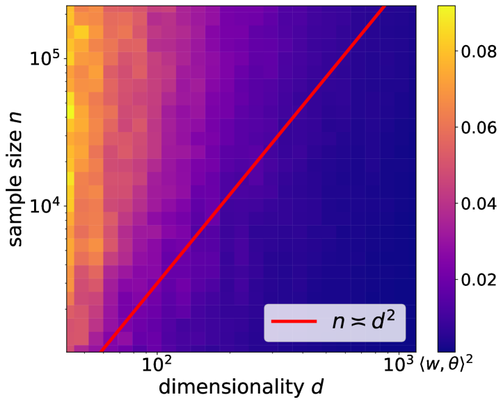
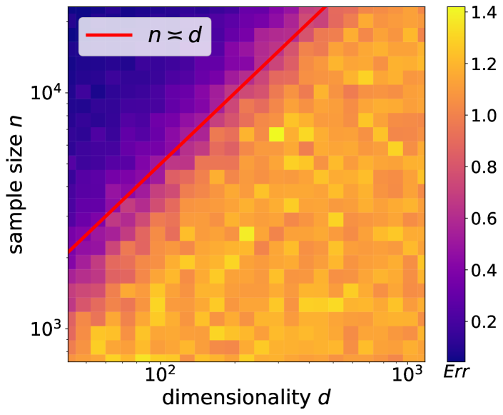
Empirically, the separation between one-pass (online) and multi-pass SGD is clearly observed in Figure 1, where we trained the same two-layer ReLU neural network to learn a single-index polynomial with information exponent $p=3$. We see that SGD with reused batch (Figure 1(b)) reaches low generalization error using roughly $n\asymp d$ samples, whereas online SGD fails to achieve even weak recovery with much larger sample size $n=\Omega(d^{2})$. Our main contribution is to establish this near-optimal sample complexity for two-layer NNs trained by a variant of SGD with reused training data.

1.1 Our Contributions

We answer the above question in the affirmative by showing that for (1.1) with arbitrary polynomial link function, SGD training on a natural class of shallow NNs can achieve small generalization error using polynomial compute and $n=\tilde{O}(d)$ training examples, if we employ a layer-wise optimization procedure (analogous to that in [BES+22, DLS22, AAM23]) and reuse of the same minibatch:

Theorem (informal).

A shallow NN with $N=\tilde{O}_{d}(1)$ neurons can learn arbitrary single-index polynomials up to small population loss: $\mathbb{E}_{\boldsymbol{x}}[(f_{\boldsymbol{\Theta}}(\boldsymbol{x})-f_{*}(\boldsymbol{x}))^{2}]=o_{d,\mathbb{P}}(1)$, using $n=\tilde{O}_{d}(d)$ samples, and an SGD-based algorithm (with reused training data) minimizing the squared loss objective in $T=\tilde{O}_{d}(d)$ gradient steps.

We make the following remarks on our main result.

  • The theorem suggests that NN + SGD with reused batch can match the statistical efficiency of SQ algorithms tailored for low-dimensional polynomial regression [CM20]. Furthermore, the sample complexity is information theoretically optimal up to polylogarithmic factors, and surpasses the CSQ lower bound for $p>2$ (see Figure 2); this disproves a conjecture in [AAM23] stating that $n\asymp d^{p/2}$ is the optimal sample complexity for empirical risk minimization with SGD.

  • A key observation in our analysis is that with suitable activation function, SGD with reused batch can go beyond correlational queries and implement (a subclass of) SQ algorithms. This enables polynomial transformations to the labels that reduce the information exponent to (at most) 2, and hence optimization can escape the high-entropy “equator” at initialization in polylogarithmic time.

Upon completion of this work, we became aware of the preprint [ADK+24] showing weak recovery with similar sample complexity, also by exploiting the reuse of training data. Our work was conducted independently and simultaneously, and their contribution is not reflected in the present manuscript (beyond this paragraph).

Information theoretic limitSGD + batch reuse [This work] SQ algorithm [CM20]Smoothed SGD [DNGL23] CSQ lower bound [DLS22]One-pass SGD [BAGJ21]Kernel methods [GMMM21]$d$ $\tilde{\Theta}(d)$ $\tilde{\Theta}(d^{p/2})$ $\tilde{\Theta}(d^{p-1})$ $\Theta(d^{q})$
Figure 2: Sample complexity of learning single-index model where the link function $\sigma_{*}$ has degree $q$ and information exponent $p$. For the CSQ lower bound, we translate the tolerance to sample complexity using the i.i.d. concentration heuristic $\tau\approx n^{-1/2}$. We restrict ourselves to algorithms using polynomial compute; this excludes the sphere-covering procedure in [DPVLB24] or exponential-width neural network in [Bac17, TS24].

2 Problem Setting and Prior Works

Notations.

$\|\cdot\|$ denotes the $\ell_{2}$ norm for vectors and the $\ell_{2}\to\ell_{2}$ operator norm for matrices. $O_{d}(\cdot)$ and $o_{d}(\cdot)$ stand for the big-O and little-o notations, where the subscript highlights the asymptotic variable $d$ and suppresses dependence on $p,q$; we write $\tilde{O}(\cdot)$ when (poly-)logarithmic factors are ignored. $\mathcal{O}_{d,\mathbb{P}}(\cdot)$ (resp. $o_{d,\mathbb{P}}(\cdot)$) represents big-O (resp. little-o) in probability as $d\to\infty$. $\Omega(\cdot),\Theta(\cdot)$ are defined analogously. $\gamma$ is the standard Gaussian distribution in $\mathbb{R}$. We denote the $L^{2}$-norm of a function $f$ with respect to the data distribution (which will be specified) as $\mathopen{}\mathclose{{}\left\|{f}}\right\|_{L^{2}}$. For $g:\mathbb{R}\to\mathbb{R}$, we denote $g^{i}$ as its $i$-th exponentiation, and $g^{(i)}$ is the $i$-th derivative. We say an event happens with high probability when the failure probability is bounded by $\operatorname{exp}\mathopen{}\mathclose{{}\left({-C\log d}}\right)$ for large constant $C$.

2.1 Complexity of Learning Single-index Models

We aim to learn a single-index model (1.1) where the link function $\sigma_{*}$ is a degree-$q$ polynomial with information exponent $p$ defined as follows.

Definition 1 (Information exponent [BAGJ21]).

Let $\{\mathsf{He}_{j}\}_{j=0}^{\infty}$ denote the normalized Hermite polynomials. The information exponent of $g\in L^{2}(\gamma)$, denoted by $\mathrm{IE}(g):=p\in\mathbb{N}_{+}$, is the index of the first non-zero Hermite coefficient of $g$, that is, given the Hermite expansion $g(z)=\sum_{i=0}^{\infty}\alpha_{i}\mathsf{He}_{i}(z)$, $p:=\min\{i>0:\alpha_{i}\neq 0\}$.

By definition we always have $p\leq q$. Note that $f_{*}$ contains $\Theta(d)$ parameters to be estimated, and hence information theoretically $n\gtrsim d$ samples are both sufficient and necessary for learning [MM18, BKM+19, DPVLB24]; however the sample complexity achieved by different (polynomial time) learning algorithms depends on structure of the link function.

  • Kernel Methods. Rotationally invariant kernels cannot adapt to the low-dimensional structure of single-index $f_{*}$ and hence suffer from the curse of dimensionality [YS19, GMMM21, DWY21, BES+22]. By a standard dimension argument [KMS20, HSSVG21, AAM22], we know that in the isotropic data setting, kernel methods (including neural networks in the lazy regime [JGH18, COB19]) require $n\gtrsim d^{q}$ samples to learn degree-$q$ polynomials in $\mathbb{R}^{d}$.

  • Gradient-based Training of NNs. While NNs can easily approximate a single-index model [Bac17], the statistical complexity of gradient-based learning established in prior works scales as $n\gtrsim d^{\Theta(p)}$: in the well-specified setting, [BAGJ21] proved a sample complexity of $n=\tilde{\Theta}(d^{p-1})$ for online SGD, which is later improved to $\tilde{\Theta}(d^{p/2})$ by a smoothed objective [DNGL23]; as for the misspecified setting, [BBSS22, DKL+23] showed that $n\gtrsim d^{p}$ samples suffice, and in some cases a $\tilde{\Theta}(d^{p-1})$ complexity is achievable [AAM23, OSSW24]. Consequently, at the information-theoretic limit ($n\asymp d$), existing results can only cover the learning of low information exponent targets [AAM22, BMZ23, BES+23]. It is worth noting that this exponential dependence on $p$ also appears in the CSQ lower bounds [DLS22, AAM22], which is often considered to be indicative of the performance of SGD learning with the squared loss (see Section 2.2).

  • Statistical Query Learners. If we do not restrict ourselves to correlational queries, then (1.1) can be efficiently solved near the information-theoretic limit. Specifically, [CM20] proposed an SQ algorithm that learns any single-index polynomials using $n=\tilde{O}(d)$ samples; the key ingredient is to construct nonlinear transformations to the labels that lowers the information exponent to $2$ (similar preprocessing also appeared in context of phase retrieval [MM18, BKM+19]). This is consistent with the recently established SQ lower bound [DPVLB24], which suggests a statistical complexity independent of the information exponent $p$ when $\sigma_{*}$ is polynomial.

2.2 Can Gradient Descent Go Beyond Correlational Queries?

Correlational statistical query.

A statistical query (SQ) learner [Kea98, Rey20] accesses the target $f_{*}$ through noisy queries $\tilde{\phi}$ with error tolerance $\tau$: $|\tilde{\phi}-\mathbb{E}_{\boldsymbol{x},y}[\phi(\boldsymbol{x},y)]|\leq\tau$. Lower bound on the performance of SQ algorithm is a classical measure of computational hardness. In the context of gradient-based optimization, an often-studied subclass of SQ is the correlational statistical query (CSQ) [BF02] where the query is restricted to (noisy version of) $\mathbb{E}_{\boldsymbol{x},y}[\phi(\boldsymbol{x})y]$. To see the connection between CSQ and SGD, consider the gradient of expected squared loss for one neuron $f_{\boldsymbol{w}}(\boldsymbol{x})$:

$\displaystyle\nabla_{\boldsymbol{w}}\mathbb{E}_{\boldsymbol{x},y}(f_{\boldsymbol{w}}(\boldsymbol{x})-y)^{2}\propto-\mathbb{E}_{\boldsymbol{x},y}[\underbrace{y\cdot\nabla_{\boldsymbol{w}}f_{\boldsymbol{w}}(\boldsymbol{x})}_{\text{correlational query}}]\,+\,\mathbb{E}_{\boldsymbol{x}}[\underbrace{f_{\boldsymbol{w}}(\boldsymbol{x})\cdot\nabla_{\boldsymbol{w}}f_{\boldsymbol{w}}(\boldsymbol{x})}_{\text{\!\!\!\!can be evaluated without $y$\!\!\!\!}}].$ (2.1)

One can see that information of the target function is encoded in the correlation term in the gradient. To infer the statistical efficiency of GD in the empirical risk minimization setting, we replace the population gradient with the empirical average $\nabla_{\boldsymbol{w}}(\frac{1}{n}\sum_{i=1}^{n}(f_{\boldsymbol{w}}(\boldsymbol{x}_{i})-y_{i})^{2})$, and heuristically equate the CSQ tolerance $\tau$ with the scale of i.i.d. concentration error $n^{-1/2}$.

For the Gaussian single-index model class with information exponent $p$, [DLS22] proved a lower bound stating that a CSQ learner either has access to queries with tolerance $\tau\lesssim d^{-p/4}$, or exponentially many queries are needed to learn $f_{*}$ with small population loss. Using the heuristic $\tau\approx n^{-1/2}$, this suggests a sample complexity lower bound $n\gtrsim d^{p/2}$ for polynomial time CSQ algorithm. This lower bound can be achieved by a landscape smoothing procedure [DNGL23] (in the well-specified setting), and is conjectured to be optimal for empirical risk minimization with SGD [AAM23].

SGD with reused data.

As discussed in Section 2.1, the gap between SQ and CSQ algorithms primarily stems from the existence of label transformations that decrease the information exponent. While such transformation cannot be utilized by a CSQ learner, [DTA+24] argued that they may arise from two consecutive gradient updates using the same minibatch. For illustrative purposes, consider an example where one neuron $f_{\boldsymbol{w}}(\boldsymbol{x})=\sigma(\langle\boldsymbol{x},\boldsymbol{w}\rangle)$ is updated by two GD steps using the same training example $(\boldsymbol{x},y)$, starting from zero initialization $\boldsymbol{w}^{0}=\mathbf{0}$ (we focus on the correlational term in the loss for simplicity):

$\displaystyle\!\!\!\boldsymbol{w}^{2}=$ $\displaystyle~{}\boldsymbol{w}^{1}+\eta\cdot y\sigma^{\prime}(\langle\boldsymbol{x},\boldsymbol{w}^{1}\rangle)\boldsymbol{x}=\eta\sigma^{\prime}(0)\underbrace{y\cdot\boldsymbol{x}}_{\text{\!\!\!CSQ term\!\!\!}}+~{}\eta\underbrace{y\sigma^{\prime}(\eta\sigma^{\prime}(0)\mathopen{}\mathclose{{}\left\|{\boldsymbol{x}}}\right\|^{2}\cdot y)\boldsymbol{x}}_{\text{non-CSQ term}}.$ (2.2)

Under appropriate learning rate scaling $\eta\cdot\mathopen{}\mathclose{{}\left\|{\boldsymbol{x}}}\right\|^{2}=\Theta(1)$, one can see that in the second gradient step, the label $y$ is transformed by the nonlinearity $\sigma^{\prime}$, even though the loss function itself is not modified. Based on this observation, [DTA+24] showed that if the non-CSQ term in (2.2) reduces the information exponent to $1$, then weak recovery (i.e., nontrivial overlap between the first-layer parameters $\boldsymbol{w}$ and index features $\boldsymbol{\theta}$) can be achieved after two GD steps with $n=\Theta(d)$ samples.

2.3 Challenges in Establishing Statistical Guarantees

Importantly, the analysis in [DTA+24] does not lead to concrete learnability guarantees for the class of single-index polynomials for the following reasons: $(i)$ it is not clear if an appropriate nonlinear transformation that lowers the information exponent can always be extracted from SGD with reused batch, and $(ii)$ the weak recovery guarantee may not translate to a sample complexity for the trained NN to achieve small generalization error. We elaborate these technical challenges below.

SGD decreases information exponent.

To show weak recovery, [DTA+24, Definition 3.1] assumed that the student activation $\sigma$ can reduce the information exponent of the labels to $1$; while a few examples are given (e.g., odd-degree Hermite polynomials), the existence of such transformations in SGD is not guaranteed:

  • The label transformation employed in prior SQ algorithms [CM20] is based on thresholding, which reduces the information exponent to $2$ for any polynomial $\sigma_{*}$; however, isolating such function from SGD updates on the squared loss is challenging. Instead, we show in Proposition 5 that monomial transformation suffices, and it can be extracted from SGD via Taylor expansion.

  • If the link function $\sigma_{*}$ is even, then its information exponent after arbitrary nonlinear transformation is at least $2$; such functions are predicted not be not learnable by SGD in the $n\asymp d$ regime [DTA+24]. To handle this setting, we analyze the SGD update up to $\mathrm{polylog}(d)$ time, at which a nontrivial overlap can be established by a Grönwall-type argument similar to [BAGJ21]. This recovers results on phase retrieval when $\sigma_{*}(z)=z^{2}$ which requires $n=\Omega(d\log d)$.

From weak recovery to sample complexity.

Note that weak recovery (i.e., $|\langle\boldsymbol{w},\boldsymbol{\theta}\rangle|>\varepsilon$ for some small constant $\varepsilon>0$) is generally insufficient to establish low generalization error of the trained NN. Therefore, we need to show that starting from a nontrivial overlap, subsequent gradient steps can achieve strong recovery of the index features (i.e., $|\langle\boldsymbol{w},\boldsymbol{\theta}\rangle|>1-\varepsilon$), despite the link misspecification. After the first-layer parameters align with the target function, we can train the second-layer parameters with SGD to learn the link function $\sigma_{*}$ with the aid of random bias units.

3 SGD Achieves Almost-linear Sample Complexity

We consider the learning of single-index polynomials with degree $q$ and information exponent $p$:

Assumption 1.

The target function is given as $f_{*}(\boldsymbol{x})=\sigma_{*}(\langle\boldsymbol{x},\boldsymbol{\theta}\rangle)$, where the link function $\sigma_{*}:\mathbb{R}\to\mathbb{R}$ admits the Hermite decomposition $\sigma_{*}(z)=\sum_{i=p}^{q}\alpha_{i}\mathsf{He}_{i}(z)$.

3.1 Training Algorithm

We train the following two-layer neural network with $N$ neurons using SGD to minimize the squared loss:

$\displaystyle f_{\boldsymbol{\Theta}}(\boldsymbol{x})=\frac{1}{N}\sum_{j=1}^{N}a_{j}\sigma_{j}(\langle\boldsymbol{x},\boldsymbol{w}_{j}\rangle+b_{j}),$ (3.1)

where $\boldsymbol{\Theta}=(\boldsymbol{w}_{j},a_{j},b_{j})_{j=1}^{N}$ are trainable parameters, and $\sigma_{j}:\mathbb{R}\to\mathbb{R}$ is the activation function defined as the sum of Hermite polynomials up to degree $C_{\sigma}$: $\sigma_{j}(z):=\sum_{i=0}^{C_{\sigma}}\beta_{j,i}\mathsf{He}_{i}(z)$, where $C_{\sigma}$ only depends on the degree of link function $\sigma_{*}$. Note that we allow each neuron to have a different nonlinearity as indicated by the subscript in $\sigma_{j}$; this subscript is omitted when we focus on the dynamics of one single neuron. Our SGD training procedure is described in Algorithm 1, and below we outline the key ingredients of the algorithm.

  • Algorithm 1 employs a layer-wise training strategy common in the recent feature learning theory literature [DLS22, BES+22, BBSS22, AAM23, MHWSE23], where in the first stage, we optimize the first-layer parameters $\{\boldsymbol{w}_{j}\}_{j=1}^{N}$ with normalized SGD to learn the low-dimensional latent representation (index features $\boldsymbol{\theta}$), and in the second phase, we train the second-layer $\{a_{j}\}_{j=1}^{N}$ to fit the unknown link function $\sigma_{*}$.

  • The most important part in Phase I of Algorithm 1 is the reuse of the same minibatch in the gradient computation. Specifically, we sample a fresh batch of training examples in every two GD steps; this enables us to extract non-CSQ terms from two consecutive gradient updates outlined in (2.2).

  • We introduce an interpolation step between the current and previous iterates with hyperparameter $\xi$ to stabilize the training dynamics; this resembles a negative momentum term often seen in optimization algorithms [AZ18, ZLBH19]; the role of this interpolation step is discussed in Section 4.2. We also use a projected gradient update $\tilde{\nabla}_{\boldsymbol{w}}\mathcal{L}(\boldsymbol{w})=(\boldsymbol{I}_{d}-\boldsymbol{w}^{2t}{\boldsymbol{w}^{2t}}^{\top})\nabla_{\boldsymbol{w}}\mathcal{L}(\boldsymbol{w})$ for steps $2t$ and $2t+1$, where $\nabla_{\boldsymbol{w}}$ is the Euclidean gradient. Similar use of projection also appeared in [DNGL23, AAM23].

1
Input : Learning rates $\eta^{t}$, momentum parameters $\{\xi_{j}^{t}\}_{j=1}^{N}$, number of steps $T_{1},T_{2}$,
$\ell_{2}$ regularization $\lambda$.
2
3Initialize $\boldsymbol{w}^{0}_{j}\sim\mathbb{S}^{d-1}(1)$, $a_{j}\sim\mathrm{Unif}\{\pm r_{a}\}$.
4Phase I: normalized SGD on first-layer parameters
5       for $t=0$ to $T_{1}$ do
6             if $t>0$ is even then
7                   Draw i.i.d. sample $(\boldsymbol{x},y)$.
8                   Interpolate ${\boldsymbol{w}}^{t}_{j}\leftarrow\boldsymbol{w}^{t}_{j}-\xi_{j}^{t}(\boldsymbol{w}^{t}_{j}-\boldsymbol{w}^{t-2}_{j})$.
9                   Normalize $\boldsymbol{w}^{t}_{j}\leftarrow\boldsymbol{w}^{t}_{j}/\|\boldsymbol{w}^{t}_{j}\|$.
10            $\boldsymbol{w}^{t+1}_{j}\leftarrow\boldsymbol{w}^{t}_{j}-\eta^{t}\tilde{\nabla}_{\boldsymbol{w}}(f_{\boldsymbol{\Theta}}(\boldsymbol{x})-y)^{2},\quad(j=1,\dots,N)$.
11      
12
13Initialize $b_{j}\sim\mathrm{Unif}([-C_{b},C_{b}])$.
14Phase II: SGD on second-layer parameters
15       $\hat{\boldsymbol{a}}\leftarrow\mathrm{argmin}_{\boldsymbol{a}\in\mathbb{R}^{N}}\frac{1}{T_{2}}\sum_{i=1}^{T_{2}}\mathopen{}\mathclose{{}\left(f_{\boldsymbol{\Theta}}(\boldsymbol{x}_{i})-y_{i}}\right)^{2}+\lambda\|\boldsymbol{a}\|^{2}.$
16
Output : Prediction function $\boldsymbol{x}\mapsto f_{\hat{\boldsymbol{\Theta}}}(\boldsymbol{x})$ with $\hat{\boldsymbol{\Theta}}=(\hat{a}_{j},\boldsymbol{w}^{T_{1}}_{j},b_{j})_{j=1}^{N}$.
Algorithm 1 Gradient-based training of two-layer neural network

3.2 Convergence and Statistical Complexity

Weak Recovery Guarantee.

We first consider the “search phase” of SGD, and show that after running Phase I of Algorithm 1 for $T=\mathrm{polylog}(d)$ steps, a subset of parameters $\boldsymbol{w}$ achieve nontrivial overlap with the target direction $\boldsymbol{\theta}$. We denote $H(g;j)$ as the $j$-th Hermite coefficient of some $g\in L^{2}(\gamma)$. Our main theorems handle polynomial activations satisfying the following condition.

Assumption 2.

We require the activation function to be a polynomial $\sigma(z)=\sum_{i=0}^{C_{\sigma}}\beta_{i}\mathsf{He}_{i}(z)$ and its degree $C_{\sigma}$ to be sufficiently large so that $C_{\sigma}\geq C_{q}$ holds ($C_{q}$ is defined in Proposition 5). For all $2\leq\ell\leq C_{\sigma}$ and $k=0,1$, we assume that $H\big{(}\sigma^{(\ell)}(\sigma^{(1)})^{\ell-1};k\big{)}\neq 0$.

More precisely, a given $\sigma_{*}$, the above condition only needs to be met for one pair of $(k,\ell)$, as specified in Appendix B.1. We show that this condition is satisfied for a wide range of polynomials with degree $C_{\sigma}$.

Lemma 2.

Given any $\ell\geq 2$ and $k\geq 0$. For $C_{\sigma}\geq\frac{2\ell+k-1}{\ell}$, if we choose $\{\beta_{i}\}_{i=0}^{C_{\sigma}}$ where each $\beta_{i}$ is randomly drawn from some interval $[a_{i},b_{i}]$ with $a_{i}<b_{i}$, then $H(\sigma^{(\ell)}(\sigma^{(1)})^{\ell-1};k)\neq 0$ with probability one.

The following theorem states that $n=\tilde{\Theta}(d)$ samples are sufficient to achieve weak recovery.

Theorem 1.

Under Assumptions 1 and 2, for suitable choices of hyperparameters $\eta^{t}=\tilde{O}_{d}(Nd^{-1})$ and $\xi_{j}^{t}=O(1)$, there exists constant $C(q)$ such that after Phase I of Algorithm 1 is run for $2T_{1,1}=C(q)\cdot d\mathrm{polylog}(d)$ steps, with high probability, there exists a subset of neurons $\boldsymbol{w}_{j}^{2T_{1}}\in\mathcal{W}$ with $|\mathcal{W}|=\tilde{\Theta}(N)$ such that $\big{|}\langle\boldsymbol{w}_{j}^{2T_{1}},\boldsymbol{\theta}\rangle\big{|}>c$ for some $c\gtrsim 1/\mathrm{polylog}(d)$.

Recall that at random initialization we have $\langle\boldsymbol{w},\boldsymbol{\theta}\rangle\approx d^{-1/2}$ with high probability. The theorem hence implies that SGD “escapes from mediocrity” after seeing $n=\tilde{O}(d)$ samples, analogous to the information exponent $p=2$ setting studied in [BAGJ21]. We remark that due to the small second-layer initialization, the squared loss is dominated by the correlation loss, which allows us to track the evolution of each neuron independently; similar use of vanishing initialization also appeared in [BES+22, AAM23].

Strong recovery and sample complexity.

After weak recovery is achieved, we continue Phase I to amplify the alignment. Due to the nontrivial overlap between $\boldsymbol{w}$ and $\boldsymbol{\theta}$, the objective is no longer dominated by the lowest degree in the Hermite expansion. Therefore, to establish strong recovery ($\langle\boldsymbol{w},\boldsymbol{\theta}\rangle>1-\varepsilon$), we place an additional assumption on the activation function.

Assumption 3.

Recall the Hermite expansions $\sigma_{*}(z)=\sum_{i=p}^{q}\alpha_{i}\mathsf{He}_{i}(z)$, $\sigma_{j}(z)=\sum_{i=0}^{C_{\sigma}}\beta_{j,i}\mathsf{He}_{i}(z)$, we assume the coefficients satisfy $\alpha_{i}\beta_{j,i}\geq 0$ for $p\leq i\leq q$.

This assumption is easily verified in the well-specified setting $\sigma_{*}=\sigma$ [BAGJ21] since $\alpha_{i}=\beta_{i}$, and under link misspecification, it has been directly assumed in prior work [MHWSE23]. We follow [OSSW24] and show that by randomizing the Hermite coefficients of the activation function, a subset of neurons satisfy the above assumption for any degree-$q$ polynomial link function $\sigma_{*}$.

Lemma 3.

If we set $\sigma_{j}(z)=\sum_{i=0}^{C_{\sigma}}\beta_{j,i}\mathsf{He}_{i}(z)$, where for each neuron we sample $\beta_{j,i}\stackrel{{\scriptstyle\mathrm{\tiny{i.i.d.}}}}{{\sim}}\mathrm{Unif}(\{\pm r_{i}\})$ with appropriate constant $r_{i}$, then Assumption 2 and 3 are satisfied in $\operatorname{exp}\mathopen{}\mathclose{{}\left({-\Theta(q)}}\right)$-fraction of neurons.

The proof is found in Appendix B.1. Note that in our construction of activation functions for both assumptions, we do not exploit knowledge of the link function $\sigma_{*}$ other than its degree $q$ which decides the constant $C_{\sigma}$. The next theorem shows that by running Phase I for $\tilde{\Theta}(d)$ more steps, a subset of neurons can achieve almost perfect overlap with the index features.

Theorem 2.

For student neurons with activation satisfying Assumptions 2 and 3 and parameter $\boldsymbol{w}_{j}$ starting from a nontrivial overlap $c$ specified in Theorem 1, for suitable hyperparameters $\eta^{t}=\tilde{O}_{d}(Nd^{-1})$ and $\xi_{j}^{t}=1-\tilde{O}(\varepsilon)$, if we continue to run Phase I of Algorithm 1 for $2T_{1,2}=\tilde{\Theta}_{d}(d\varepsilon^{-2})$ steps, then we achieve $\big{\langle}\boldsymbol{w}_{j}^{2(T_{1,1}+T_{1,2})},\boldsymbol{\theta}\big{\rangle}>1-\varepsilon$ with high probability.

Combining Theorem 1,2 and Lemma 3, we know that after $T_{1}=2(T_{1,1}+T_{1,2})$ steps, there exists some constant $C(q)$ depending only on the degree $q$ such that $1/(C(q)\cdot\mathrm{polylog}(d))$ fraction of the neurons become $\varepsilon$-close to the target direction $\boldsymbol{\theta}$. The following proposition shows that after strong recovery, training the second-layer parameters in Phase II is sufficient for the NN model (3.1) to achieve small generalization error.

Proposition 4.

After Phase I terminates, for suitable $\lambda>0$, the output of Phase II satisfies

$$\mathbb{E}_{\boldsymbol{x}}[(f_{\hat{\boldsymbol{\Theta}}}(\boldsymbol{x})-f_{*}(\boldsymbol{x}))^{2}]\lesssim\varepsilon.$$

with probability 1 as $d\to\infty$, if we set $T_{2}=C(q)N^{4}\mathrm{polylog}(d)\varepsilon^{-2}$, $N=C(q)\mathrm{polylog}(d)\varepsilon^{-1}$ for some constant $C(q)$ depending on the target degree $q$.

Putting things together.

Combining the above theorems, we conclude that in order for two-layer NN (3.1) trained by Algorithm 1 to achieve $\varepsilon$ population squared loss, it is sufficient to set

$\displaystyle n=T_{1}+T_{2}\asymp C(q)\cdot(d\varepsilon^{-2}\vee\varepsilon^{-6})\mathrm{polylog}(d),\quad N\asymp C(q)\cdot\varepsilon^{-1}\mathrm{polylog}(d),$ (3.2)

where constant $C(q)$ only depends on the target degree $q$ (although exponentially). Hence we may set $\varepsilon^{-1}\asymp\mathrm{polylog}d$ to conclude an almost-linear sample and computational complexity for learning arbitrary single-index polynomials up to $o_{d}(1)$ population error. This establishes the informal theorem in Section 1.

4 Proof Sketch

In this section we outline the high-level ideas and key steps in our derivation.

4.1 Monomial Transformation Reduces Information Exponent

To prove the main theorem, we first establish the existence of nonlinear label transformation that $(i)$ reduces the information exponent, and $(ii)$ can be easily extracted from SGD updates. If we ignore desideratum $(ii)$, then for polynomial link functions, transformations that decrease the information exponent to at most $2$ have been constructed in [CM20, Section 2.1]. However, prior results are based on the thresholding function with specific offset, and it is not clear if such function naturally arises from SGD with batch reuse. The following proposition shows that the effect of thresholding can also be achieved by a simple monomial transformation.

Proposition 5.

Let $f:\mathbb{R}\to\mathbb{R}$ be any polynomial with degree up to $p$ and $\mathopen{}\mathclose{{}\left\|{f}}\right\|_{L^{2}(\gamma)}^{2}=1$, then

  • (i)

    There exists some $i\leq C_{q}\in\mathbb{N}_{+}$ such that ${\mathrm{IE}}(f^{i})\leq 2$, where constant $C_{q}$ only depends on $q$.

  • (ii)

    Let $f^{\mathrm{odd}}:\mathbb{R}\to\mathbb{R}$ be the odd part of $f$ with $\mathbb{E}_{t\sim\mathcal{N}(0,\boldsymbol{I}_{d})}[f^{\mathrm{odd}}(t)^{2}]\geq\rho>0$. Then there exists some $i\leq C_{q,\rho}\in\mathbb{N}_{+}$ such that ${\mathrm{IE}}(f^{i})=1$, where constant $C_{q,\rho}$ only depends on $q$ and $\rho$.

We make the following remarks.

  • The proposition implies that for any polynomial link function that is not even, there exists some power $i\in\mathbb{N}_{+}$ only depending on the degree of $\sigma_{*}$ such that raising the function to the $i$-the power reduces the information exponent to $1$. For even link functions, the information exponent after arbitrary transformation is at least $2$, and this lowest value can also be achieved by monomial transformation. Furthermore, we provide a uniform upper-bound on the required degree of transformation $i$ via a compactness argument.

  • The advantage of working with monomial transformations is that they can be obtained from two GD steps on the same training example, by Taylor expanding the activation $\sigma^{\prime}$. In Section 4.2, we build upon this observation to show that Phase I of Algorithm 1 achieves weak recovery using $n\gtrsim d\,\mathrm{polylog}(d)$ samples.

Intuition behind the analysis.

Our proof is inspired by [CM20] which introduced a (non-polynomial) label transformation that reduces the information exponent of any degree-$q$ polynomial to at most $2$. To prove the existence of monomial transformation for the same purpose, we first show that for a fixed link function $\sigma_{*}$, there exists some $i$ such that the $i$-th power of the link function has information exponent $2$, which mirrors the transformation used in [CM20]. Then, we make use of the compactness of the space of link functions to define a test function and obtain a uniform bound on $i$. As for the polynomial transformation for non-even functions, we exploit the asymmetry of $\sigma_{*}$ to further reduce the information exponent to 1.

4.2 SGD with Batch Reuse Implements Polynomial Transformation

Now we present a more formal discussion of (2.2) to illustrate how polynomial transformation can be utilized in batch reuse SGD. We let $\eta^{t}\equiv\eta$. When one neuron $f_{\boldsymbol{w}}(\boldsymbol{x})=\sigma(\langle\boldsymbol{x},\boldsymbol{w}\rangle)$ is updated by two GD steps using the same sample $(\boldsymbol{x},y)$, starting from $\boldsymbol{w}^{0}:=\boldsymbol{\omega}$, the alignment with $\boldsymbol{\theta}$ becomes

$\displaystyle\langle\boldsymbol{\theta},\boldsymbol{w}^{2}\rangle=\mathopen{}\mathclose{{}\left\langle\boldsymbol{\theta},\big{[}\boldsymbol{w}^{1}+\eta\cdot y\sigma^{\prime}(\langle\boldsymbol{x},\boldsymbol{w}^{1}\rangle)\boldsymbol{x}\big{]}}\right\rangle=\langle\boldsymbol{\theta},\boldsymbol{\omega}\rangle+$ (4.1)
$\displaystyle\eta\bigg{[}y\sigma^{\prime}(\langle\boldsymbol{\omega},\boldsymbol{x}\rangle)\langle\boldsymbol{\theta},\boldsymbol{x}\rangle+\sum_{i=0}^{C_{\sigma}-1}\underbrace{(\eta\|\boldsymbol{x}\|^{2})^{i}y^{i+1}(i!)^{-1}(\sigma^{\prime}(\langle\boldsymbol{\omega},\boldsymbol{x}\rangle))^{i}\sigma^{(i+1)}(\langle\boldsymbol{\omega},\boldsymbol{x}\rangle)\langle\boldsymbol{\theta},\boldsymbol{x}\rangle}_{=:\psi_{i}}\bigg{]}.$ (4.2)

We take $\eta\leq c_{\eta}d^{-1}$ with a small constant $c_{\eta}$ so that $\eta\|\boldsymbol{x}\|^{2}\ll 1$. Crucially, the strength of each term in (4.2) can vary depending on properties of the link function $\sigma_{*}$, which is unknown. Hence a careful analysis is required to ensure that the suitable monomial transformation is always singled out from the gradient update. We therefore divide our analysis into four cases (for simplicity we present the noiseless setting below).

  • (I)

    If $\mathrm{IE}(\sigma_{*})=1$. All terms in the summation in (4.2) with $i\geq 2$ decay as fast as $\eta\|\boldsymbol{x}\|^{2}\ll 1$. On the other hand, the expectation of $y\sigma^{\prime}(\langle\boldsymbol{\omega},\boldsymbol{x}\rangle)\langle\boldsymbol{\theta},\boldsymbol{x}\rangle$ is roughly $\alpha_{1}\beta_{1}\gtrsim 1$. Therefore we may isolate the informative term $y\sigma^{\prime}(\langle\boldsymbol{\omega},\boldsymbol{x}\rangle)\langle\boldsymbol{\theta},\boldsymbol{x}\rangle$. This case is discussed in Section B.3.3.

  • (II)

    Else if $\mathrm{IE}((\sigma_{*})^{I})=1$ for some $2\leq I\leq C_{\sigma}$. Let $I$ be the lowest degree of monomial transformation such that $\mathrm{IE}((\sigma_{*})^{I})=1$. Since $\sigma_{*},\cdots,\sigma_{*}^{I-1}$ have information exponent larger than $1$, expectations of $y\sigma^{\prime}(\langle\boldsymbol{\omega},\boldsymbol{x}\rangle)\langle\boldsymbol{\theta},\boldsymbol{x}\rangle$ and $\psi_{i}\ (i=2,\cdots,I-2)$ scales as $\langle\boldsymbol{\theta},\boldsymbol{\omega}\rangle\asymp d^{-1/2}$. For $i=I-1$, because $\sigma_{*}^{I}$ has information exponent $1$,

    $\displaystyle\mathbb{E}[\psi_{I-1}]=\,$ $\displaystyle\mathbb{E}\big{[}(\eta\|\boldsymbol{x}\|^{2})^{I-1}y^{I}((I-1)!)^{-1}(\sigma^{(1)}(\langle\boldsymbol{\omega},\boldsymbol{x}\rangle))^{I-1}\sigma^{(I)}(\langle\boldsymbol{\omega},\boldsymbol{x}\rangle)\langle\boldsymbol{\theta},\boldsymbol{x}\rangle\big{]}$ (4.3)
    $\displaystyle\asymp\,$ $\displaystyle c_{\eta}^{I-1}H(\sigma_{*}^{I};1)H(\sigma^{(I)}(\sigma^{(1)})^{I-1};0).$ (4.4)

    For $i\geq I$, $\psi_{i}$ decays as $c_{\eta}^{I}$, which is smaller than the scale of $\psi_{I-1}\asymp c_{\eta}^{I-1}$. Hence the term $\psi_{I-1}\gtrsim c_{\eta}^{I-1}$ is singled out. This case is discussed in Section B.3.2.

  • (III)

    Else if $\mathrm{IE}(\sigma_{*})=2$. We have $\mathbb{E}[y\sigma^{\prime}(\langle\boldsymbol{\omega},\boldsymbol{x}\rangle)\langle\boldsymbol{\theta},\boldsymbol{x}\rangle]\approx 2\alpha_{2}\beta_{2}\langle\boldsymbol{\theta},\boldsymbol{\omega}\rangle$. Also, for $i\geq 2$, since $\sigma_{*}^{2},\cdots,\sigma_{*}^{C_{\sigma}}$ have information exponent at least $2$, expectation of $\psi_{i}$ is roughly of order $(\eta\|\boldsymbol{x}\|^{2})^{i}\langle\boldsymbol{\theta},\boldsymbol{\omega}\rangle$. Therefore, the term $y\sigma^{\prime}(\langle\boldsymbol{\omega},\boldsymbol{x}\rangle)\langle\boldsymbol{\theta},\boldsymbol{x}\rangle$ is singled out, and the expectation scales as $\alpha_{2}\beta_{2}d^{-1/2}$ at initialization. This case is discussed in Section B.3.3.

  • (IV)

    Else $\mathrm{IE}((\sigma_{*})^{I})=2$ for some $2\leq I\leq C_{\sigma}$. In this case, since $\sigma_{*},\cdots,\sigma_{*}^{I-1}$ have information exponent larger than $2$, expectations of $y\sigma^{\prime}(\langle\boldsymbol{\omega},\boldsymbol{x}\rangle)\langle\boldsymbol{\theta},\boldsymbol{x}\rangle$ and $\psi_{i}\ (i=2,\cdots,I-2)$ are at most $(\langle\boldsymbol{\theta},\boldsymbol{\omega}\rangle)^{2}\asymp d^{-1}$. And at $i=I-1$, because $\sigma_{*}^{I}$ has information exponent $2$,

    $\displaystyle\mathbb{E}[\psi_{I-1}]=\,$ $\displaystyle\mathbb{E}\big{[}(\eta\|\boldsymbol{x}\|^{2})^{I-1}y^{I}((I-1)!)^{-1}(\sigma^{(1)}(\langle\boldsymbol{\omega},\boldsymbol{x}\rangle))^{I-1}\sigma^{(I)}(\langle\boldsymbol{\omega},\boldsymbol{x}\rangle)\langle\boldsymbol{\theta},\boldsymbol{x}\rangle\big{]}$ (4.5)
    $\displaystyle\asymp\,$ $\displaystyle c_{\eta}^{I-1}H(\sigma_{*}^{I};2)H(\sigma^{(I)}(\sigma^{(1)})^{I-1};1)\langle\boldsymbol{\theta},\boldsymbol{\omega}\rangle.$ (4.6)

    As for $i\geq I$, because $\sigma_{*}^{i}$ has information exponent larger than $1$ for $I+1\leq i\leq C_{\sigma}$, $\psi_{i}$ decays as $c_{\eta}^{I}\langle\boldsymbol{\theta},\boldsymbol{\omega}\rangle$, which is smaller than $\psi_{I-1}\asymp c_{\eta}^{I-1}\langle\boldsymbol{\theta},\boldsymbol{\omega}\rangle$. Thus, the term $\psi_{I-1}$ is dominating, whose scale is roughly $c_{\eta}^{I-1}d^{-1/2}$ at initialization. This case is discussed in Section B.3.1.

Why interpolation is required.

In all the cases above, strength of the signal is at least $\eta c_{\eta}^{I-1}d^{-1/2}$ at initialization. However, this signal strength may not dominate the error coming from discarding the effect of normalization. Usually, given the gradient $-\boldsymbol{g}$ and projection $P_{\boldsymbol{w}}=\boldsymbol{I}_{d}-\boldsymbol{w}\boldsymbol{w}^{\top}$, the spherical gradient affects the alignment as $\langle\boldsymbol{\theta},\boldsymbol{w}^{t+1}\rangle=\big{\langle}\boldsymbol{\theta},\frac{\boldsymbol{w}^{t}+\eta P_{\boldsymbol{w}}\boldsymbol{g}}{\|\boldsymbol{w}^{t}+\eta P_{\boldsymbol{w}}\boldsymbol{g}\|}\big{\rangle}\geq\langle\boldsymbol{\theta},\boldsymbol{w}^{t}\rangle+\eta\langle\boldsymbol{\theta},\boldsymbol{g}\rangle-\frac{1}{2}\eta^{2}\|\boldsymbol{g}\|^{2}\langle\boldsymbol{\theta},\boldsymbol{w}^{t}\rangle+\text{(negligible terms)}$, see [BAGJ21] or discussion in [DNGL23]. Here $\eta\langle\boldsymbol{\theta},\boldsymbol{g}\rangle$ corresponds to the signal, and $-\frac{1}{2}\eta^{2}\|\boldsymbol{g}\|^{2}\langle\boldsymbol{\theta},\boldsymbol{w}^{t}\rangle$ comes from the normalization. Thus, taking $\eta$ sufficiently small, the normalization term shrinks faster than the signal. However, in our setting, the signal shrinks at the rate of $\eta^{I}$, and hence taking a smaller step does not improve the signal-to-noise ratio. The interpolation step in our analysis allows us to reduce the effect of normalization without shrinking the signal too much, by ensuring $\boldsymbol{w}^{2(t+1)}$ stays close to $\boldsymbol{w}^{2t}$.

Combining the four cases yields the following lemma on the evolution of alignment.

Lemma 6.

Under the assumptions per Theorem 1, one of the following holds:

  • (i)

    $\langle\boldsymbol{\theta},\boldsymbol{w}_{j}^{2(t+1)}\rangle\geq\langle\boldsymbol{\theta},\boldsymbol{w}_{j}^{2t}\rangle+\eta^{2t}_{j}(1-\xi_{j}^{2(t+1)})\gamma+\eta^{2t}_{j}(1-\xi_{j}^{2(t+1)})\nu^{2t}_{j}.$

  • (ii)

    $\langle\boldsymbol{\theta},\boldsymbol{w}_{j}^{2(t+1)}\rangle\geq\langle\boldsymbol{\theta},\boldsymbol{w}_{j}^{2t}\rangle+\eta^{2t}_{j}(1-\xi_{j}^{2(t+1)})\gamma\langle\boldsymbol{\theta},\boldsymbol{w}_{j}^{2t}\rangle+\eta^{2t}_{j}(1-\xi_{j}^{2(t+1)})\nu^{2t}_{j}.$

Here $\gamma\gtrsim c_{\eta}^{I-1}$ is a constant that depends on $\sigma_{*}$ and $\nu^{2t}_{j}$ is a mean-zero noise.

For (i), taking expectation immediately yields that weak recovery is achieved within $(\eta(1-\xi)\gamma)^{-1}=\tilde{O}(d)$ steps. For (ii), $\langle\boldsymbol{\theta},\boldsymbol{w}_{j}^{2t}\rangle=:\kappa^{t}$ can be approximated by a differential equation $\frac{\mathrm{d}\kappa^{t}}{\mathrm{d}t}=\eta(1-\xi)\gamma\kappa^{t}$. Solving this yields $\kappa^{t}=\kappa^{0}\exp(\eta(1-\xi)\gamma t)\approx d^{-\frac{1}{2}}\exp(\eta(1-\xi)\gamma t)$, and weak recovery is obtained within $t\lesssim(\eta(1-\xi)\gamma)^{-1}\cdot\log d=\tilde{O}(d)$ steps, similar to the analysis in [BAGJ21].

4.3 Analysis of Phase II and Statistical Guarantees

Once strong recovery is achieved for the first-layer parameters, we turn to Phase II and optimize the second-layer with $\ell_{2}$ regularization. Since the objective is strongly convex, gradient-based optimization can efficiently minimize the empirical loss. The learnability guarantee follows from standard analysis analogous to that in [AAM22, DLS22, BES+22], where we construct a “certificate” second-layer $\boldsymbol{a}^{*}\in\mathbb{R}^{N}$ that achieves small loss and small norm:

$$\textstyle\mathbb{E}_{\boldsymbol{x}}\mathopen{}\mathclose{{}\left(f_{*}(\boldsymbol{x})-\frac{1}{N}\sum_{j=1}^{N}a^{*}_{j}\sigma_{j}\big{(}\langle{\boldsymbol{w}_{j}^{T_{1}}},\boldsymbol{x}\rangle+b_{j}\big{)}}\right)^{2}\leq\varepsilon^{*},\quad\|\boldsymbol{a}^{*}\|\lesssim r^{*},$$

from which the population loss of the regularized empirical risk minimizer can be bounded via standard Rademacher complexity argument. To construct such a certificate, we make use of the random bias units $\{b_{j}\}_{j=1}^{N}$ to approximate the link function $\sigma_{*}$ as done in [DLS22, BBSS22, OSSW24].

5 Conclusion and Future Directions

In this work we showed that a two-layer neural network (3.1) trained by SGD with reused batch can learn arbitrary single-index polynomials up to $\varepsilon$ population error using $n=\tilde{O}(d\varepsilon^{-2})$ samples and compute. Our analysis is based on the observation that by reusing the same minibatch twice in the gradient computation, a non-correlational term arises in the SGD update that transforms the labels (despite the loss function is not modified). Specifically, following the definition in [DPVLB24], we know that polynomial $\sigma_{*}$ has generative exponent at most $2$, which implies the existence of nonlinear transformation $\mathcal{T}:\mathbb{R}\to\mathbb{R}$ such that the information exponent $p_{*}$ becomes at most $2$, i.e.,

$$\mathbb{E}[\mathcal{T}(y)\mathsf{He}_{i}(\langle\boldsymbol{x},\boldsymbol{\theta}\rangle)]\neq 0,\quad\text{for $i=1$ or $2$.}$$

We show that restricting $\mathcal{T}$ to be polynomial is sufficient, and such transformation can be extracted by Taylor-expanding the SGD update. Then we show via careful analysis of the trajectory that strong recovery and low population error can be achieved under suitable activation function.

Future directions.

First, our analysis only handles link functions with generative exponent $p_{*}\leq 2$; while this covers arbitrary polynomial $\sigma_{*}$ analogous to [CM20], it is interesting to examine whether SGD with reused batch can learn targets with $p_{*}\geq 3$ with a sample complexity matching the SQ lower bound. It is also possible that ERM algorithms on i.i.d. data can achieve a statistical complexity beyond the SQ lower bound due to non-adversarial noise [DH21, DH24]; such mechanism is not exploited in our current analysis. Additional interesting directions include extension to multi-index [BAGJ22, BBPV23, CWPPS23, Gla23], hierarchical polynomials [NDL23], and additive models [OSSW24]. Lastly, the SGD algorithm that we employ requires a layer-wise training procedure and a specific batch reuse schedule; one may therefore ask if standard multi-pass SGD training of all parameters simultaneously (as reported in Figure 1) also achieves the same statistical efficiency.


Acknowledgements

The authors thank Gerard Ben Arous, Joan Bruna, Alex Damian, Marco Mondelli, and Eshaan Nichani for the discussions and feedback on the manuscript. JDL acknowledges support of the ARO under MURI Award W911NF-11-1-0304, NSF CCF 2002272, NSF IIS 2107304, NSF CIF 2212262, ONR Young Investigator Award, and NSF CAREER Award 2144994. KO was partially supported by JST ACT-X (JPMJAX23C4). TS was partially supported by JSPS KAKENHI (24K02905) and JST CREST (JPMJCR2015).


References

  • [AAM22] Emmanuel Abbe, Enric Boix Adsera, and Theodor Misiakiewicz. The merged-staircase property: a necessary and nearly sufficient condition for sgd learning of sparse functions on two-layer neural networks. In Conference on Learning Theory, pages 4782–4887. PMLR, 2022.
  • [AAM23] Emmanuel Abbe, Enric Boix Adsera, and Theodor Misiakiewicz. SGD learning on neural networks: leap complexity and saddle-to-saddle dynamics. In The Thirty Sixth Annual Conference on Learning Theory, pages 2552–2623. PMLR, 2023.
  • [ADK+24] Luca Arnaboldi, Yatin Dandi, Florent Krzakala, Luca Pesce, and Ludovic Stephan. Repetita iuvant: Data repetition allows sgd to learn high-dimensional multi-index functions. arXiv preprint arXiv:2405.15459, 2024.
  • [AZ18] Zeyuan Allen-Zhu. Katyusha: The first direct acceleration of stochastic gradient methods. Journal of Machine Learning Research, 18(221):1–51, 2018.
  • [Bac17] Francis Bach. Breaking the curse of dimensionality with convex neural networks. The Journal of Machine Learning Research, 18(1):629–681, 2017.
  • [BAGJ21] Gerard Ben Arous, Reza Gheissari, and Aukosh Jagannath. Online stochastic gradient descent on non-convex losses from high-dimensional inference. The Journal of Machine Learning Research, 22(1):4788–4838, 2021.
  • [BAGJ22] Gerard Ben Arous, Reza Gheissari, and Aukosh Jagannath. High-dimensional limit theorems for sgd: Effective dynamics and critical scaling. Advances in Neural Information Processing Systems, 35:25349–25362, 2022.
  • [BBPV23] Alberto Bietti, Joan Bruna, and Loucas Pillaud-Vivien. On learning Gaussian multi-index models with gradient flow. arXiv preprint arXiv:2310.19793, 2023.
  • [BBSS22] Alberto Bietti, Joan Bruna, Clayton Sanford, and Min Jae Song. Learning single-index models with shallow neural networks. Advances in Neural Information Processing Systems, 35:9768–9783, 2022.
  • [BES+22] Jimmy Ba, Murat A Erdogdu, Taiji Suzuki, Zhichao Wang, Denny Wu, and Greg Yang. High-dimensional asymptotics of feature learning: How one gradient step improves the representation. Advances in Neural Information Processing Systems, 35:37932–37946, 2022.
  • [BES+23] Jimmy Ba, Murat A Erdogdu, Taiji Suzuki, Zhichao Wang, and Denny Wu. Learning in the presence of low-dimensional structure: A spiked random matrix perspective. In Thirty-seventh Conference on Neural Information Processing Systems, 2023.
  • [BF02] Nader H Bshouty and Vitaly Feldman. On using extended statistical queries to avoid membership queries. Journal of Machine Learning Research, 2(Feb):359–395, 2002.
  • [BKM+19] Jean Barbier, Florent Krzakala, Nicolas Macris, Léo Miolane, and Lenka Zdeborová. Optimal errors and phase transitions in high-dimensional generalized linear models. Proceedings of the National Academy of Sciences, 116(12):5451–5460, 2019.
  • [BL20] Yu Bai and Jason D. Lee. Beyond linearization: On quadratic and higher-order approximation of wide neural networks. In International Conference on Learning Representations, 2020.
  • [BMZ23] Raphaël Berthier, Andrea Montanari, and Kangjie Zhou. Learning time-scales in two-layers neural networks. arXiv preprint arXiv:2303.00055, 2023.
  • [CCM11] Seok-Ho Chang, Pamela C Cosman, and Laurence B Milstein. Chernoff-type bounds for the Gaussian error function. IEEE Transactions on Communications, 59(11):2939–2944, 2011.
  • [CM20] Sitan Chen and Raghu Meka. Learning polynomials in few relevant dimensions. In Conference on Learning Theory, pages 1161–1227. PMLR, 2020.
  • [COB19] Lenaic Chizat, Edouard Oyallon, and Francis Bach. On lazy training in differentiable programming. Advances in Neural Information Processing Systems, 32, 2019.
  • [CWPPS23] Elizabeth Collins-Woodfin, Courtney Paquette, Elliot Paquette, and Inbar Seroussi. Hitting the high-dimensional notes: An ode for sgd learning dynamics on glms and multi-index models. arXiv preprint arXiv:2308.08977, 2023.
  • [DH21] Rishabh Dudeja and Daniel Hsu. Statistical query lower bounds for tensor pca. Journal of Machine Learning Research, 22(83):1–51, 2021.
  • [DH24] Rishabh Dudeja and Daniel Hsu. Statistical-computational trade-offs in tensor pca and related problems via communication complexity. The Annals of Statistics, 52(1):131–156, 2024.
  • [DKL+23] Yatin Dandi, Florent Krzakala, Bruno Loureiro, Luca Pesce, and Ludovic Stephan. Learning two-layer neural networks, one (giant) step at a time. arXiv preprint arXiv:2305.18270, 2023.
  • [DLS22] Alexandru Damian, Jason Lee, and Mahdi Soltanolkotabi. Neural networks can learn representations with gradient descent. In Conference on Learning Theory, pages 5413–5452. PMLR, 2022.
  • [DNGL23] Alex Damian, Eshaan Nichani, Rong Ge, and Jason D. Lee. Smoothing the landscape boosts the signal for SGD: Optimal sample complexity for learning single index models. In Thirty-seventh Conference on Neural Information Processing Systems, 2023.
  • [DPVLB24] Alex Damian, Loucas Pillaud-Vivien, Jason D Lee, and Joan Bruna. The computational complexity of learning gaussian single-index models. arXiv preprint arXiv:2403.05529, 2024.
  • [DTA+24] Yatin Dandi, Emanuele Troiani, Luca Arnaboldi, Luca Pesce, Lenka Zdeborová, and Florent Krzakala. The benefits of reusing batches for gradient descent in two-layer networks: Breaking the curse of information and leap exponents. arXiv preprint arXiv:2402.03220, 2024.
  • [DWY21] Konstantin Donhauser, Mingqi Wu, and Fanny Yang. How rotational invariance of common kernels prevents generalization in high dimensions. In International Conference on Machine Learning, pages 2804–2814. PMLR, 2021.
  • [Gla23] Margalit Glasgow. Sgd finds then tunes features in two-layer neural networks with near-optimal sample complexity: A case study in the xor problem. arXiv preprint arXiv:2309.15111, 2023.
  • [GMMM21] Behrooz Ghorbani, Song Mei, Theodor Misiakiewicz, and Andrea Montanari. Linearized two-layers neural networks in high dimension. The Annals of Statistics, 49(2):1029–1054, 2021.
  • [HSSVG21] Daniel Hsu, Clayton H Sanford, Rocco Servedio, and Emmanouil Vasileios Vlatakis-Gkaragkounis. On the approximation power of two-layer networks of random relus. In Conference on Learning Theory, pages 2423–2461. PMLR, 2021.
  • [JGH18] Arthur Jacot, Franck Gabriel, and Clément Hongler. Neural tangent kernel: Convergence and generalization in neural networks. In Advances in neural information processing systems, pages 8571–8580, 2018.
  • [Kea98] Michael Kearns. Efficient noise-tolerant learning from statistical queries. Journal of the ACM (JACM), 45(6):983–1006, 1998.
  • [KMS20] Pritish Kamath, Omar Montasser, and Nathan Srebro. Approximate is good enough: Probabilistic variants of dimensional and margin complexity. In Conference on Learning Theory, pages 2236–2262. PMLR, 2020.
  • [MHPG+23] Alireza Mousavi-Hosseini, Sejun Park, Manuela Girotti, Ioannis Mitliagkas, and Murat A Erdogdu. Neural networks efficiently learn low-dimensional representations with SGD. In The Eleventh International Conference on Learning Representations, 2023.
  • [MHWSE23] Alireza Mousavi-Hosseini, Denny Wu, Taiji Suzuki, and Murat A. Erdogdu. Gradient-based feature learning under structured data. In Thirty-seventh Conference on Neural Information Processing Systems (NeurIPS 2023), 2023.
  • [MM18] Marco Mondelli and Andrea Montanari. Fundamental limits of weak recovery with applications to phase retrieval. In Conference On Learning Theory, pages 1445–1450. PMLR, 2018.
  • [NDL23] Eshaan Nichani, Alex Damian, and Jason D Lee. Provable guarantees for nonlinear feature learning in three-layer neural networks. Advances in Neural Information Processing Systems, 36, 2023.
  • [O’D14] Ryan O’Donnell. Analysis of Boolean Functions. Cambridge University Press, 2014.
  • [OSSW24] Kazusato Oko, Yujin Song, Taiji Suzuki, and Denny Wu. Learning sum of diverse features: computational hardness and efficient gradient-based training for ridge combinations. In Conference on Learning Theory. PMLR, 2024.
  • [Rey20] Lev Reyzin. Statistical queries and statistical algorithms: Foundations and applications. arXiv preprint arXiv:2004.00557, 2020.
  • [Sch80] Jacob T Schwartz. Fast probabilistic algorithms for verification of polynomial identities. Journal of the ACM (JACM), 27(4):701–717, 1980.
  • [TS24] Shokichi Takakura and Taiji Suzuki. Mean-field analysis on two-layer neural networks from a kernel perspective. arXiv preprint arXiv:2403.14917, 2024.
  • [WWF24] Zhichao Wang, Denny Wu, and Zhou Fan. Nonlinear spiked covariance matrices and signal propagation in deep neural networks. In Conference on Learning Theory. PMLR, 2024.
  • [YS19] Gilad Yehudai and Ohad Shamir. On the power and limitations of random features for understanding neural networks. Advances in Neural Information Processing Systems, 32, 2019.
  • [ZLBH19] Michael Zhang, James Lucas, Jimmy Ba, and Geoffrey E Hinton. Lookahead optimizer: k steps forward, 1 step back. Advances in neural information processing systems, 32, 2019.

Appendix A Polynomial Transformation

Proof of Proposition 5. We use a thresholding and compactness argument inspired by [CM20].

A.1 Proof for Even Functions $(i)$

We divide the analysis into the following steps.

(i-1): Monomials reducing the information exponent. Define $\tau(f)=\max_{-2\leq t\leq 2}|f(t)|$. This entails that if $|f(t)|\geq\tau(f)$, then we have $|t|>2$.

Consider the following expectation:

$\displaystyle\mathbb{E}_{t\sim\mathcal{N}(0,\boldsymbol{I}_{d})}\bigg{[}\bigg{(}\frac{f(t)}{2\tau(f)}\bigg{)}^{i}(t^{2}-1)\bigg{]}.$ (A.1)

We evaluate the case when $i$ is even. (A.1) can be lower bounded as

(A.1)=italic-(A.1italic-)absent\displaystyle\eqref{eq:PT-1}= $\displaystyle~{}\mathbb{E}_{t\sim\mathcal{N}(0,\boldsymbol{I}_{d})}\bigg{[}\mathbbm{1}[|f(t)|\geq 2\tau(f)]\bigg{(}\frac{f(t)}{2\tau(f)}\bigg{)}^{i}(t^{2}-1)\bigg{]}$ (A.2)
$\displaystyle\quad+\mathbb{E}_{t\sim\mathcal{N}(0,\boldsymbol{I}_{d})}\bigg{[}\mathbbm{1}[\tau(f)\leq|f(t)|<2\tau(f)]\bigg{(}\frac{f(t)}{2\tau(f)}\bigg{)}^{i}(t^{2}-1)\bigg{]}$ (A.3)
$\displaystyle\quad+\mathbb{E}_{t\sim\mathcal{N}(0,\boldsymbol{I}_{d})}\bigg{[}\mathbbm{1}[|f(t)|<\tau(f)]\bigg{(}\frac{f(t)}{2\tau(f)}\bigg{)}^{i}(t^{2}-1)\bigg{]}$ (A.4)
$\displaystyle\geq$ $\displaystyle~{}\mathbb{E}_{t\sim\mathcal{N}(0,\boldsymbol{I}_{d})}\bigg{[}\mathbbm{1}[|f(t)|\geq 2\tau(f)]\bigg{(}\frac{2\tau(f)}{2\tau(f)}\bigg{)}^{i}(2^{2}-1)\bigg{]}$ (A.5)
$\displaystyle\quad+\mathbb{E}_{t\sim\mathcal{N}(0,\boldsymbol{I}_{d})}\bigg{[}\mathbbm{1}[\tau(f)\leq|f(t)|<2\tau(f)]\bigg{(}\frac{f(t)}{2\tau(f)}\bigg{)}^{i}(2^{2}-1)\bigg{]}$ (A.6)
$\displaystyle\quad+\mathbb{E}_{t\sim\mathcal{N}(0,\boldsymbol{I}_{d})}\bigg{[}\mathbbm{1}[|f(t)|<\tau(f)]\bigg{(}\frac{\tau(f)}{2\tau(f)}\bigg{)}^{i}(0^{2}-1)\bigg{]}$ (A.7)
$\displaystyle\geq$ $\displaystyle~{}3\mathbb{P}_{t\sim\mathcal{N}(0,\boldsymbol{I}_{d})}[|f(t)|\geq 2\tau(f)]-2^{-i}.$ (A.8)

Note that $\mathbb{P}[|f(t)|\geq 2\tau(f)]$ is positive (since $f$ is polynomial) and independent of $i$, while $2^{-i}$ decays to 00 as $i$ increases. Therefore, for sufficiently large $i\in\mathbb{N}$, (A.1) is positive and hence ${\mathrm{IE}}(f^{i})\leq 2$. The subsequent analysis aims to provide an upper bound on $i$.

(i-2): Construction of test function. We introduce the notation $H(\cdot;j)$ which takes any function (in $L^{1}$) and returns its $j$-th Hermite coefficient. We consider the following test function:

$\displaystyle\mathscr{H}(f):=\sum_{i=2}^{\infty}\bigg{(}\frac{H(f^{i};2)}{2^{\frac{i}{2}}(2i-1)^{\frac{iq}{2}}}\bigg{)}^{2}.$ (A.9)

(i-3): Lower bound of test function via compactness. Let $\mathcal{F}_{q}$ be a set of polynomials with degree up to $q$ with unit $L^{2}$ norm. Because $\mathscr{H}(f)$ is positive for any $f\in\mathcal{F}_{q}$, $H(f^{i};2)$ is continuous with respect to $f$, and $\mathcal{F}_{q}$ is a compact set, $\inf_{f\in\mathcal{F}_{q}}\mathscr{H}(f)$ admits a minimum value $\mathscr{H}_{0}$ which is positive.

(i-4): Conclusion via hypercontractivity. Because $f$ is a polynomial with degree at most $q$, Gaussian hypercontractivity [O’D14] yields that

$\displaystyle 2H(f^{i};2)^{2}\leq\mathbb{E}_{t\sim\mathcal{N}(0,\boldsymbol{I}_{d})}\big{[}(f(t))^{2i}\big{]}\leq(2i-1)^{iq}\big{(}\mathbb{E}_{t\sim\mathcal{N}(0,\boldsymbol{I}_{d})}\big{[}f(t)^{2}\big{]}\big{)}^{i}=(2i-1)^{iq}.$ (A.10)

Therefore, for all polynomials in $\mathcal{F}_{q}$, a partial sum of (A.9) is uniformly bounded by

$\displaystyle\bigg{|}\sum_{i=j}^{\infty}\bigg{(}\frac{H(f^{i};2)}{2^{\frac{i}{2}}(2i-1)^{\frac{iq}{2}}}\bigg{)}^{2}\bigg{|}\leq\sum_{i=j}^{\infty}2^{-i-1}=2^{-j}\to 0\quad(j\to\infty).$ (A.11)

Combining this with the fact that $\mathscr{H}(f)\geq\mathscr{H}_{0}>0$, we know that there exists some $C_{q}\leq 1+\log_{2}(\mathscr{H}_{0}^{-1})$ such that

$\displaystyle\sum_{i=2}^{C_{q}}\bigg{(}\frac{H(f^{i};2)}{2^{\frac{i}{2}}(2i-1)^{\frac{iq}{2}}}\bigg{)}^{2}>\frac{1}{2}\mathscr{H}_{0}>0,$ (A.12)

for all polynomials in $\mathcal{F}_{q}$. This means that there is at least one $i\leq C_{q}$ such that $H(f^{i};2)\neq 0$.

A.2 Proof for Non-even Functions $(ii)$

(ii-1): Monomials reducing the information exponent. We prove that some exponentiation of $g:=f^{2}$ has non-zero first Hermite coefficient. Denote $g^{\mathrm{odd}}$ as the odd part of $g$, and similarly $g^{\mathrm{even}}$. Let $\upsilon(g)\in\mathbb{R}_{+}$ be the value at which the followings hold:

  • (a)

    $g^{\mathrm{odd}}(t)>0$ for all $t\geq\upsilon(g)$ and $g^{\mathrm{odd}}(t)<0$ for all $t\leq-\upsilon(g)$.

  • (b)

    $g^{\mathrm{even}}(t)>|g^{\mathrm{odd}}(t)|$ for all $t\geq\upsilon(g)$ and $t\leq-\upsilon(g)$.

  • (c)

    For for all $t\geq\upsilon(g)$ and $t\leq-\upsilon(g)$, $g(s)=g(t)$ (as an equation of $s$) only has two real-valued solutions with opposing signs.

Such threshold $\upsilon(g)$ exists because the tail of $g=f^{2}$ is dominated by the highest degree which is even. Then, we let $\tau(g)=\max_{-\upsilon(g)\leq t\leq\upsilon(g)}|g(t)|$.

Consider the following expectation:

$\displaystyle\mathbb{E}_{t\sim\mathcal{N}(0,\boldsymbol{I}_{d})}\bigg{[}\bigg{(}\frac{g(t)}{2\tau(g)}\bigg{)}^{i}t\bigg{]}.$ (A.13)

(A.13) is decomposed as

(A.13)=italic-(A.13italic-)absent\displaystyle\eqref{eq:PT-11}= $\displaystyle~{}\mathbb{E}_{t\sim\mathcal{N}(0,\boldsymbol{I}_{d})}\bigg{[}\mathbbm{1}[|g(t)|\geq 3\tau(f)]\bigg{(}\frac{g(t)}{3\tau(g)}\bigg{)}^{i}t\bigg{]}$ (A.14)
$\displaystyle\quad+\mathbb{E}_{t\sim\mathcal{N}(0,\boldsymbol{I}_{d})}\bigg{[}\mathbbm{1}[2\tau(g)\leq|g(t)|<3\tau(g)]\bigg{(}\frac{g(t)}{3\tau(f)}\bigg{)}^{i}t\bigg{]}$ (A.15)
$\displaystyle\quad+\mathbb{E}_{t\sim\mathcal{N}(0,\boldsymbol{I}_{d})}\bigg{[}\mathbbm{1}[|g(t)|<2\tau(g)]\bigg{(}\frac{g(t)}{3\tau(g)}\bigg{)}^{i}t\bigg{]}.$ (A.16)

We first evaluate the first term. Because of (c), $g(t)=3\tau(f)$ has two real-valued solutions $\alpha<0<\beta$. Because of (a) and (b), $g(\beta)=g^{\mathrm{even}}(\beta)+g^{\mathrm{odd}}(\beta)=3\tau(f)>g^{\mathrm{even}}(-\beta)+g^{\mathrm{odd}}(-\beta)=g^{\mathrm{odd}}(-\beta)$. Because $\lim_{t\to-\infty}g^{\mathrm{odd}}(t)=+\infty$, and $\alpha$ is the only solution in $t<0$, we have $\alpha<-\beta$. Moreover, for all $t>\beta$, we have $g(t)=g^{\mathrm{even}}(t)+g^{\mathrm{odd}}(t)>g^{\mathrm{even}}(-t)+g^{\mathrm{odd}}(-t)=g^{\mathrm{odd}}(-t)$. Combining the above, the first term of (A.16) is bounded as

$\displaystyle\mathbb{E}_{t\sim\mathcal{N}(0,\boldsymbol{I}_{d})}\bigg{[}\mathbbm{1}[|g(t)|\geq 3\tau(f)]\bigg{(}\frac{g(t)}{3\tau(g)}\bigg{)}^{i}t\bigg{]}$ (A.17)
$\displaystyle=\mathbb{E}_{t\sim\mathcal{N}(0,\boldsymbol{I}_{d})}\bigg{[}\mathbbm{1}[\beta\leq t\leq-\alpha]\bigg{(}\frac{g(t)}{3\tau(g)}\bigg{)}^{i}t\bigg{]}+\mathbb{E}_{t\sim\mathcal{N}(0,\boldsymbol{I}_{d})}\bigg{[}\mathbbm{1}[t\geq-\alpha]\bigg{(}\frac{g(t)}{3\tau(g)}\bigg{)}^{i}t\bigg{]}$ (A.18)
$\displaystyle\quad+\mathbb{E}_{t\sim\mathcal{N}(0,\boldsymbol{I}_{d})}\bigg{[}\mathbbm{1}[t\leq\alpha]\bigg{(}\frac{g(t)}{3\tau(g)}\bigg{)}^{i}t\bigg{]}$ (A.19)
$\displaystyle=\mathbb{E}_{t\sim\mathcal{N}(0,\boldsymbol{I}_{d})}\big{[}\mathbbm{1}[\beta\leq t\leq-\alpha]t\big{]}+\mathbb{E}_{t\sim\mathcal{N}(0,\boldsymbol{I}_{d})}\bigg{[}\mathbbm{1}[t\geq-\alpha]\bigg{(}\bigg{(}\frac{g(t)}{3\tau(g)}\bigg{)}^{i}-\bigg{(}\frac{g(-t)}{3\tau(g)}\bigg{)}^{i}\bigg{)}t\bigg{]}$ (A.20)
$\displaystyle>\beta\mathbb{P}_{t\sim\mathcal{N}(0,\boldsymbol{I}_{d})}\big{[}\beta\leq t\leq-\alpha\big{]}.$ (A.21)

Following the exact same reasoning, we know that the second term of (A.16) is positive. Finally, the third term which is bounded by

$\displaystyle\mathbb{E}_{t\sim\mathcal{N}(0,\boldsymbol{I}_{d})}\big{[}\mathbbm{1}[|g(t)|<2\tau(g)]\bigg{(}\frac{g(t)}{3\tau(g)}\bigg{)}^{i}t\big{]}\geq-\mathbb{E}_{t\sim\mathcal{N}(0,\boldsymbol{I}_{d})}\big{[}\mathbbm{1}[|g(t)|<2\tau(g)]|t|\big{]}\bigg{(}\frac{2}{3}\bigg{)}^{i}.$ (A.22)

Putting things together,

(A.16)>βt𝒩(0,𝑰d)[βtα]𝔼t𝒩(0,𝑰d)[𝟙[|g(t)|<2τ(g)]|t|](23)i.italic-(A.16italic-)𝛽subscriptsimilar-to𝑡𝒩0subscript𝑰𝑑delimited-[]𝛽𝑡𝛼subscript𝔼similar-to𝑡𝒩0subscript𝑰𝑑delimited-[]1delimited-[]𝑔𝑡2𝜏𝑔𝑡superscript23𝑖\displaystyle\eqref{eq:PT-12}>\beta\mathbb{P}_{t\sim\mathcal{N}(0,\boldsymbol{I}_{d})}\big{[}\beta\leq t\leq-\alpha\big{]}-\mathbb{E}_{t\sim\mathcal{N}(0,\boldsymbol{I}_{d})}\big{[}\mathbbm{1}[|g(t)|<2\tau(g)]|t|\big{]}\bigg{(}\frac{2}{3}\bigg{)}^{i}. (A.23)

The first term is independent of $i$ and positive, while the second term goes to zero as $i$ grows. Therefore, there exists some $i$ such that $\mathrm{IE}(g^{i};1)=1$.

(ii-2): Construction of test function. This time we consider the following function:

$\displaystyle\mathscr{H}(f):=\sum_{i=2}^{\infty}\bigg{(}\frac{H(f^{i};1)}{2^{\frac{i}{2}}(2i-1)^{\frac{iq}{2}}}\bigg{)}^{2}.$ (A.24)

(ii-3): Lower bound of test function via compactness. Let $\mathcal{F}_{q}$ be a set of unit $L^{2}$-norm polynomials with degree up to $q$ and $\mathbb{E}_{t\sim\mathcal{N}(0,\boldsymbol{I}_{d})}[f^{\mathrm{odd}}(t)^{2}]\geq c$. Since $\mathscr{H}(f)$ is always positive for $\mathcal{F}_{q}$, $\mathscr{H}(f)$ is continuous with respect to $f$, and $\mathcal{F}_{q}$ is a compact set, $\inf_{f\in\mathcal{F}_{q}}\mathscr{H}(f)$ has the minimum value $\mathscr{H}_{0}$ that is positive. Note that $\mathscr{H}(f)$ might depends on $c$.

(ii-4): Conclusion via hypercontractivity. Using the same argument as in (i), we conclude that there exists some $C_{q,c}$ such that

$\displaystyle\sum_{i=2}^{C_{q}}\bigg{(}\frac{H(f^{i};1)}{2^{i}(2i-1)^{\frac{iq}{2}}}\bigg{)}^{2}>\frac{1}{2}\mathscr{H}_{0}>0.$ (A.25)

Because $\mathscr{H}_{0}$ depends on $c$, $C_{q,c}$ depends on $c$ as well as $q$. ∎

Appendix B SGD with Reused Batch

In this section we establish the statistical and computational complexity of Algorithm 1. Recall that the algorithm first trains the first-layer parameters with $T_{1}$ steps of SGD update, where we reuse the same sample for two consecutive steps. The analysis of first-layer training is divided into two phases: $(i)$ weak recovery ($\boldsymbol{w}^{\top}\boldsymbol{\theta}\geq\varepsilon$), and $(ii)$ strong recovery ($\boldsymbol{w}^{\top}\boldsymbol{\theta}\geq 1-\varepsilon$). We then train the second-layer parameters after strong recovery is achieved.

The section is organized as follows.

  • Section B.1 verifies the conditions on the activation function $\sigma$ to guarantee weak and strong recovery.

  • Section B.2 isolates a (nearly) constant fraction of neurons at initialization with an alignment $\boldsymbol{w}^{\top}\boldsymbol{\theta}$ above a certain threshold. We focus on such neurons in Phase I of first-layer training.

  • Section B.3 lower bounds the expected update of alignment $\boldsymbol{w}^{\top}\boldsymbol{\theta}$ of two gradient steps, and Section B.4 shows that neurons yield weak recovery within $2T_{1,1}=\tilde{O}(d)$ steps.

  • Section B.5 discusses how to convert weak recovery to strong recovery using $2T_{1,2}=\tilde{O}(d\varepsilon^{-2})$ SGD steps.

  • Finally, Section B.6 analyzes the second-layer training and concludes the proof.

In the following proofs, we introduce constants $c_{i}$ and $C_{i}$, which depends on $d$ at most polylogarithmically. Specifically, the asymptotic strength of the constants is ordered as follows.

$\displaystyle 1\simeq C_{1}\lesssim c_{1}^{-1}\lesssim C_{2}\lesssim C_{3}\lesssim c_{2}^{-1}$ (B.1)

$c_{\eta}$ in the main text can be taken as $c_{\eta}=c_{1}$, where $c_{1}$ should satisfy $\lim_{d\to\infty}c_{1}=0$, but the convergence can be arbitrarily slow. This requirement comes from the fact that we do not know the exact value of $H(\sigma_{*}^{I};k_{*})$, which might be very small. To ensure that the signal is isolated, taking $\eta\asymp c_{1}d^{-1}$ with arbitrarily slow $c_{1}$ suffices. $C_{2}$ can also be arbitrarily slow, as long as it satisfies $C_{2}=\mathrm{poly}(c_{1}^{-1})$. $C_{3}=\mathrm{polylog}(d)$ will be used to represent polylogarithmic factor that comes from high probability bounds.

B.1 Conditions on the Activation Function

B.1.1 Verifying Assumption 2

In the following, we focus on the activation function of a single neuron and omit the subscript that distinguishes different neurons. Recall that we consider polynomial activation functions written as

$\displaystyle\sigma(z):=\sum_{j=0}^{C_{\sigma}}\beta_{j}\mathsf{He}_{j}(z).$ (B.2)

For weak recovery, we can use any polynomial that has degree $C_{\sigma}\geq C_{q}$ as long as the following condition holds: If $\mathrm{IE}(\sigma_{*})\geq 2$ and there exists some $i\leq C_{\sigma}$ such that $\mathrm{IE}(\sigma_{*}^{i})=1$, $\sigma$ should satisfy

$\displaystyle H\bigg{(}\frac{1}{(I-1)!}\sigma^{(I)}(\sigma^{(1)})^{I-1};0\bigg{)}\neq 0.$ (B.3)

If $\mathrm{IE}(\sigma_{*})\geq 3$ and there does not exist any $i\leq C_{\sigma}$ such that $\mathrm{IE}(\sigma_{*}^{i})=1$ (in this case there exists some $i\leq C_{q}$ such that $\mathrm{IE}(\sigma_{*}^{i})=2$), $\sigma$ should satisfy

$\displaystyle H\bigg{(}\frac{1}{(I-1)!}\sigma^{(I)}(\sigma^{(1)})^{I-1};1\bigg{)}\neq 0.$ (B.4)

Below we prove Lemma 2 which shows that the above conditions are met with probability $1$ for randomly drawn the Hermite coefficients.

Proof of Lemma 2. We note that $H(\sigma^{(i)}(\sigma^{(1)})^{i-1};k)=\mathbb{E}[\sigma^{(i)}(\sigma^{(1)})^{i-1}\mathsf{He}_{k}]$ is a polynomial of $\{\beta_{j}\}_{j=0}^{C_{\sigma}}$. This polynomial is not identically equal to zero. To confirm this, consider $\sigma=x^{C_{\sigma}}+x^{C_{\sigma}-1}$. Because $\sigma^{(i)}(\sigma^{(1)})^{i-1}$ is expanded as a sum of $x^{l}(i(C_{\sigma}-3)\leq l\leq i(C_{\sigma}-2)+1$ with positive coefficients and each $x^{l}$ is a sum of $\mathsf{He}_{l},\mathsf{He}_{l-2}\cdots$ with positive coefficients, $\sigma^{(i)}(\sigma^{(1)})^{i-1}$ has all positive Hermite coefficients for degree $0,1,\cdots,i(C_{\sigma}-2)+1$. If $k\leq i(C_{\sigma}-2)+1$, this choice of $\sigma$ yields $H(\sigma^{(i)}(\sigma^{(1)})^{i-1};k)>0$, which confirms that $H(\sigma^{(i)}(\sigma^{(1)})^{i-1};k)$ as a polynomial of $\{\beta_{j}\}_{j=0}^{C_{\sigma}}$ is not identically equal to zero.

Now, the assertion follows from the Schwartz–Zippel Lemma [Sch80], or the fact that zeros of a non-zero polynomial form a measure-zero set. ∎

B.1.2 Verifying Assumption 3

On the other hand, for the strong recovery we require an additional condition on the activation function due to link misspecification, which is also introduced in [BAGJ21, MHWSE23]:

$\displaystyle\sum_{j=p}^{p}j!\alpha_{j}\beta_{j}s^{j}>0\quad\text{for all $s>0$}.$ (B.5)

In order to meet Assumption 2 and (3) simultaneously, we follow [OSSW24] and randomize the activation function. Specifically, the activation function should satisfy

  • (I)

    If $\mathrm{IE}(\sigma_{*})=1$. We require $\beta_{1}>0$ and $\sum_{j=1}^{q}j!\alpha_{j}\beta_{j}s^{j-1}>0$ for all $s>0$.

  • (II)

    Else if $\mathrm{IE}((\sigma_{*})^{I})=1$ for some $2\leq I\leq C_{\sigma}$. We require $H(\sigma^{(I)}(\sigma^{(1)})^{I-1};0)$ is not 00 and has the same sign as $H((\sigma_{*})^{I};1)$. Also, $\sum_{j=2}^{q}j!\alpha_{j}\beta_{j}s^{j-1}>0$ for all $s>0$.

  • (III)

    Else if $\mathrm{IE}(\sigma_{*})=2$. We require $\beta_{2}>0$ and $\sum_{j=2}^{q}j!\alpha_{j}\beta_{j}s^{j-1}>0$ for all $s>0$.

  • (IV)

    Else $\mathrm{IE}((\sigma_{*})^{I})=2$ for some $2\leq I\leq C_{q}$. We require $H(\sigma^{(I)}(\sigma^{(1)})^{I-1};1)$ is not 00 and has the same sign as $H((\sigma_{*})^{I};2)$. Also, $\sum_{j=3}^{q}j!\alpha_{j}\beta_{j}s^{j-1}>0$ for all $s>0$.

Now we prove Lemma 3 which verifies the existence of an activation function that satisfies the assumptions above with non-zero probability. The construction does not depend on the link function itself, but only its degree $q$.

Proof of Lemma 3. Let $c$ be a sufficiently small constant, and $C_{\sigma}$ be the minimum odd integer with $C_{\sigma}\geq\max\{C_{q}+1,q+2,3\}$. With probability $1/2$, we choose the coefficients as $\beta_{1}\sim\mathrm{Unif}(\{\pm 1\})$, and $\beta_{j}\sim\mathrm{Unif}(\{-c,c\})$ for $2\leq j\leq C_{\sigma}$. Then, it is easy to see (I) and (III) are met with probability at least $2^{-q}$, because they hold when $\mathrm{sign}(\alpha_{j})=\mathrm{sign}(\beta_{j})$ holds in the summation.

By taking $c$ sufficiently small, we have

$\displaystyle H(\sigma^{(I)}(\sigma^{(1)})^{I-1};0)=\underbrace{i!\beta_{I}(\beta_{1})^{I-1}}_{\text{$\asymp c$}}+O(c).$ (B.6)

When $I$ is even, by adjusting the sign of $\beta_{1}$, $H(\sigma^{(I)}(\sigma^{(1)})^{I-1};0)$ is not 00 and has the same sign as $H((\sigma_{*})^{I};1)$ with probability $\frac{1}{2}$. Note that the sign of $\beta_{1}$ is independent from whether $\sum_{j=2}^{q}j!\alpha_{j}\beta_{j}s^{j-1}>0$ for all $s>0$ holds. This holds with probability at least $2^{-q+1}$. Thus we verified (II) for even $I$.

In the same vein, we can verify (IV) for even $I\leq C_{q}\leq C_{\sigma}-1$. We have

$\displaystyle H(\sigma^{(I)}(\sigma^{(1)})^{I-1};1)=\underbrace{(I+1)!\beta_{I+1}(\beta_{1})^{I-1}}_{\text{$\asymp c$}}+O(c^{2}),$ (B.7)

and (IV) can be verified using the same argument.

Otherwise (also with probability $1/2$), we choose the coefficients as $\beta_{j}\sim\mathrm{Unif}(\{-c,c\})$ for $1\leq j\leq C_{\sigma}-2$ and $\beta_{C_{\sigma}-1}=\beta_{C_{\sigma}}=\pm 1$ to verify (II) and (IV) for odd $I$. It is easy to see that $\sum_{j=2}^{q}j!\alpha_{j}\beta_{j}s^{j-1}>0$ for all $s>0$ holds for (I) and $\sum_{j=3}^{q}j!\alpha_{j}\beta_{j}s^{j-1}>0$ for all $s>0$ for (III). In addition, $H((\mathsf{He}_{C_{\sigma}}+\mathsf{He}_{C_{\sigma}-1})^{(I)}((\mathsf{He}_{C_{\sigma}}+\mathsf{He}_{C_{\sigma}-1})^{(1)})^{I-1};0)>0$ and $H((\mathsf{He}_{C_{\sigma}}+\mathsf{He}_{C_{\sigma}-1})^{(I)}((\mathsf{He}_{C_{\sigma}}+\mathsf{He}_{C_{\sigma}-1})^{(1)})^{I-1};1)>0$. Therefore, by taking $c$ sufficiently small, flipping the sign of $\mathsf{He}_{C_{\sigma}}+\mathsf{He}_{C_{\sigma}-1}$ can change the sign of $H(\sigma^{(I)}(\sigma^{(1)})^{I-1};k)$ for both (II) and (IV) with odd $I$. Combining all cases yields the desired claim. ∎

B.2 Random Initialization

In Section B.3.1 we focus on the neurons with slightly larger initial alignment that satisfy $\kappa^{0}_{j}=\boldsymbol{\theta}^{\top}\boldsymbol{w}^{0}_{j}\geq 2C_{2}d^{-\frac{1}{2}}$ at initialization, where constant $C_{2}$ grows at most polylogarithmically in $d$. The following lemma states that roughly a constant portion of the neurons satisfies this initial alignment condition.

Lemma 7.

At the time of initialization, $\kappa^{0}_{j}=\boldsymbol{\theta}^{\top}\boldsymbol{w}^{0}$ satisfies the following:

$\displaystyle\mathbb{P}[\kappa^{0}_{j}\geq 2C_{2}d^{-\frac{1}{2}}]=\mathbb{P}[\kappa^{0}_{j}\leq-2C_{2}d^{-\frac{1}{2}}]\gtrsim e^{-16C_{2}^{2}}=\tilde{\Omega}(1).$ (B.8)

We make use of the following lemma.

Lemma 8 (Theorem 2 of [CCM11]).

For any $\beta>1$ and $s\in\mathbb{R}$, we have

$\displaystyle\frac{\sqrt{2e(\beta-1)}}{2\beta\sqrt{\pi}}e^{-\frac{\beta s^{2}}{2}}\leq\int_{s}^{\infty}\frac{1}{\sqrt{2\pi}}e^{-\frac{t^{2}}{2}}\mathrm{d}t$ (B.9)

Proof of Lemma 7. Because $\kappa^{0}=v^{\top}w\overset{\mathrm{d}}{=}\frac{{\sf e}_{1}^{\top}g}{g}$, where $g\sim\mathcal{N}(0,\boldsymbol{I}_{d})$,

$\displaystyle\mathbb{P}[\kappa^{0}_{j}\geq 2C_{2}d^{-\frac{1}{2}}]$ $\displaystyle=\mathbb{P}_{g\sim\mathcal{N}(0,\boldsymbol{I}_{d})}\bigg{[}{\sf e}_{1}^{\top}g\geq 4C_{2}\land\|g\|\leq 2d^{\frac{1}{2}}\bigg{]}$ (B.10)
$\displaystyle\geq\mathbb{P}_{g\sim\mathcal{N}(0,\boldsymbol{I}_{d})}\bigg{[}{\sf e}_{1}^{\top}g\geq 4C_{2}\bigg{]}-\mathbb{P}_{g\sim\mathcal{N}(0,\boldsymbol{I}_{d})}\bigg{[}\|g\|\geq 2d^{\frac{1}{2}}\bigg{]}$ (B.11)
$\displaystyle\gtrsim\frac{\sqrt{2e(\beta-1)}}{2\beta\sqrt{\pi}}e^{-8\beta C_{2}^{2}}-e^{-\Omega(d)}.$ (B.12)

By letting $\beta=2$, we have that $\mathbb{P}[\kappa^{0}_{j}\geq C_{2}d^{-\frac{1}{2}}]\gtrsim e^{-16C_{2}^{2}}.$ Due to symmetry, $\mathbb{P}[\kappa^{0}_{j}\leq 2C_{2}d^{-\frac{1}{2}}]=\mathbb{P}[\kappa^{0}_{j}\geq 2C_{2}d^{-\frac{1}{2}}]$. ∎

B.3 Population Update

We first analyze the training of first-layer parameters by evaluating the expected (population) update of two gradient steps with the same training example. At each step, the parameters are updated as

$\displaystyle\boldsymbol{w}^{t+1}_{j}$ $\displaystyle\leftarrow\boldsymbol{w}^{t}_{j}-\eta^{t}\tilde{\nabla}_{\boldsymbol{w}}\big{(}(f_{\boldsymbol{\Theta}}(\boldsymbol{x})-y)^{2}\big{)}$ (B.13)
$\displaystyle=\boldsymbol{w}^{t}_{j}-\eta^{t}\tilde{\nabla}_{\boldsymbol{w}}\Bigg{(}\frac{1}{N}\sum_{j=1}^{N}a_{j}\sigma({\boldsymbol{w}_{j}^{t}}^{\top}\boldsymbol{x})\Bigg{)}^{2}+2\eta^{t}\tilde{\nabla}_{\boldsymbol{w}}\Bigg{(}y\frac{1}{N}\sum_{j=1}^{N}a_{j}\sigma({\boldsymbol{w}_{j}^{t}}^{\top}\boldsymbol{x})\Bigg{)}.$ (B.14)

While the second term scales with $\eta^{t}a_{j}^{2}=\eta^{t}c_{a}^{2}$, the third term scales with $\eta^{t}a_{j}=\eta^{t}c_{a}$. Thus, by setting the second-layer scale $c_{a}$ sufficiently small, we can ignore the interaction of neurons; similar mechanism also appeared in [BES+22, AAM23]. Specifically, in the following, we show that the strength of the signal is $\boldsymbol{\theta}^{\top}\boldsymbol{w}_{j}^{t}\gtrsim d^{-\frac{1}{2}}$. Thus, by simply letting $c_{a}\lesssim C_{3}^{-1}d^{-\frac{1}{2}}$, we can ignore the effect of the squared term. Thus we may focus on the following correlational update:

$\displaystyle\boldsymbol{w}^{t+1}_{j}\leftarrow\boldsymbol{w}^{t}_{j}+\eta^{t}\tilde{\nabla}_{\boldsymbol{w}}\Bigg{(}y\frac{1}{N}\sum_{j=1}^{N}a_{j}\sigma({\boldsymbol{w}_{j}^{t}}^{\top}\boldsymbol{x})\Bigg{)}.$ (B.15)

Due to the absence of interaction between neurons, we omit the subscript $j$ for the index of neurons and ignore the prefactor of $N$ (which can be absorbed into the learning rate); multiplying $N$ to $\eta^{t}$ specified below recovers the scaling of $\eta^{t}$ presented in the main text.

B.3.1 When $\mathrm{IE}(\sigma_{*}^{I})=2$ with $I\geq 2$

First we consider the most technically difficult case, when $\mathrm{IE}[\sigma_{*}]\geq 3$ and the information exponent cannot be lowered to 1 for $i\leq C_{\sigma}$; in this case, from Proposition 5 we know that there exists some $2\leq i\leq C_{\sigma}$ such that $\mathrm{IE}[\sigma_{*}^{i}]=2$ and we let $I$ be the first such $i$.

Without loss of generality, we assume (LHS of (B.4))>0LHS of (B.4)0(\text{LHS of \eqref{eq:condition2}})>0; the same result holds for the case of $H(\sigma_{*}^{I};2)<0$ except for the opposite sign for the second term in (B.18), by simply setting $\xi=1+\tilde{\eta}$ in the following.

Lemma 9.

Starting from $\boldsymbol{w}=\boldsymbol{\omega}$, if we choose step size $\eta=c_{a}\eta^{t}=c_{1}d^{-1}$ and negative momentum $\xi=1-\tilde{\eta}$, and assume that $C_{2}d^{-\frac{1}{2}}\leq\kappa=\boldsymbol{\theta}^{\top}\boldsymbol{\omega}\leq c_{2}$ and $\tilde{\eta}\leq c_{2}$, then the expected change in the alignment after two gradient steps on the same sample $(\boldsymbol{x},y)$ in Algorithm 1 is as follows:

$\displaystyle\boldsymbol{\theta}^{\top}\boldsymbol{w}=\boldsymbol{\theta}^{\top}\boldsymbol{\omega}+(1+O(c_{1}))\cdot\eta\tilde{\eta}c_{1}^{I-1}H\bigg{(}\frac{1}{(I-1)!}\sigma^{(I)}(\sigma^{(1)})^{I-1};1\bigg{)}H\big{(}(\sigma_{*})^{I};2\big{)}\kappa+\eta\tilde{\eta}\nu,$ (B.16)

where $\nu$ is a mean-zero random variable that satisfies $\mathbb{P}[|\nu|>s]\leq\exp(-s^{1/C_{1}}/C_{1})$ for all $s>0$.

Proof.  We first compute one gradient step from $\boldsymbol{w}=\boldsymbol{\omega}$ with a fresh sample $(\boldsymbol{x},y)$.

$\displaystyle\tilde{\nabla}_{\boldsymbol{w}}y\sigma(\boldsymbol{w}^{\top}\boldsymbol{x})=y\sigma^{\prime}(\boldsymbol{\omega}^{\top}\boldsymbol{x})\boldsymbol{x}.$ (B.17)

Then, with a projection matrix $\boldsymbol{P}_{\boldsymbol{\omega}}=I-\boldsymbol{\omega}\boldsymbol{\omega}^{\top}$, the updated parameter becomes

$\displaystyle\boldsymbol{w}\leftarrow\boldsymbol{w}+\boldsymbol{P}_{\boldsymbol{\omega}}\eta y\sigma^{\prime}(\boldsymbol{w}^{\top}\boldsymbol{x})\boldsymbol{x}=\boldsymbol{\omega}+\eta y\sigma^{\prime}(\boldsymbol{\omega}^{\top}\boldsymbol{x})\boldsymbol{P}_{\boldsymbol{\omega}}\boldsymbol{x},$ (B.18)

and the next gradient step with the same sample is computed as

$\displaystyle\tilde{\nabla}_{\boldsymbol{w}}y\sigma(\boldsymbol{w}^{\top}\boldsymbol{x})$ $\displaystyle=\eta y\sigma^{\prime}(\boldsymbol{w}^{\top}\boldsymbol{x})\boldsymbol{x}$ (B.19)
$\displaystyle=y\sigma^{\prime}\big{(}(\boldsymbol{\omega}+\eta y\sigma^{\prime}(\boldsymbol{\omega}^{\top}\boldsymbol{x})\boldsymbol{P}_{\boldsymbol{\omega}}\boldsymbol{x})^{\top}\boldsymbol{x}\big{)}\boldsymbol{x}$ (B.20)
$\displaystyle=y\sigma^{\prime}\big{(}\boldsymbol{\omega}^{\top}\boldsymbol{x}+\eta\|\boldsymbol{x}\|_{\boldsymbol{P}_{\boldsymbol{\omega}}}^{2}\sigma^{\prime}(\boldsymbol{\omega}^{\top}\boldsymbol{x})y\big{)}\boldsymbol{x},$ (B.21)

here we used the notation $\|\boldsymbol{v}\|_{\boldsymbol{A}}^{2}=\boldsymbol{v}^{\top}\boldsymbol{A}\boldsymbol{v}$ for a vector $\boldsymbol{v}\in\mathbb{R}^{d}$ and a positive symmetric matrix $\boldsymbol{A}\in\mathbb{R}^{d\times d}$. From (B.18) and (B.21), the parameter after the two steps is obtained as

$\displaystyle\boldsymbol{w}$ $\displaystyle\leftarrow\boldsymbol{w}+\tilde{\nabla}_{\boldsymbol{w}}y\sigma(\boldsymbol{w}^{\top}\boldsymbol{x})$ (B.22)
$\displaystyle=\boldsymbol{\omega}+\eta y\sigma^{\prime}(\boldsymbol{\omega}^{\top}\boldsymbol{x})\boldsymbol{P}_{\boldsymbol{\omega}}\boldsymbol{x}+\eta y\sigma^{\prime}\big{(}\boldsymbol{\omega}^{\top}\boldsymbol{x}+\eta\|\boldsymbol{x}\|_{\boldsymbol{P}_{\boldsymbol{\omega}}}^{2}\sigma^{\prime}(\boldsymbol{\omega}^{\top}\boldsymbol{x})y\big{)}\boldsymbol{P}_{\boldsymbol{\omega}}\boldsymbol{x}$ (B.23)
$\displaystyle=\boldsymbol{\omega}+\eta\boldsymbol{g},$ (B.24)

where we defined

$\displaystyle\boldsymbol{g}:=y\sigma^{\prime}(\boldsymbol{\omega}^{\top}\boldsymbol{x})\boldsymbol{P}_{\boldsymbol{\omega}}\boldsymbol{x}+y\sigma^{\prime}\big{(}\boldsymbol{\omega}^{\top}\boldsymbol{x}+\eta\|\boldsymbol{x}\|_{\boldsymbol{P}_{\boldsymbol{\omega}}}^{2}\sigma^{\prime}(\boldsymbol{\omega}^{\top}\boldsymbol{x})y\big{)}\boldsymbol{P}_{\boldsymbol{\omega}}\boldsymbol{x}.$ (B.25)

Finally, normalization yields

$\displaystyle\boldsymbol{w}$ $\displaystyle\leftarrow\frac{\boldsymbol{w}-\xi(\boldsymbol{w}-\boldsymbol{\omega})}{\|\boldsymbol{w}-\xi(\boldsymbol{w}-\boldsymbol{\omega})\|}=\frac{\boldsymbol{\omega}+\eta\tilde{\eta}\boldsymbol{g}}{\|\boldsymbol{\omega}+\eta\tilde{\eta}\boldsymbol{g}\|}.$ (B.26)

Therefore, the update of the alignment is

$\displaystyle\boldsymbol{\theta}^{\top}\boldsymbol{w}$ $\displaystyle=\frac{\kappa+\eta\tilde{\eta}\boldsymbol{\theta}^{\top}\boldsymbol{g}}{\|\boldsymbol{\omega}+\eta\tilde{\eta}\boldsymbol{g}\|}=\frac{\kappa+\eta\tilde{\eta}\boldsymbol{\theta}^{\top}\boldsymbol{g}}{(1+\eta^{2}\tilde{\eta}^{2}\|\boldsymbol{g}\|^{2})^{\frac{1}{2}}}$ (B.27)
$\displaystyle\geq\kappa+\eta\tilde{\eta}\boldsymbol{\theta}^{\top}\boldsymbol{g}-\frac{1}{2}\kappa\eta^{2}\tilde{\eta}^{2}\|\boldsymbol{g}\|^{2}-\frac{1}{2}\eta^{3}\tilde{\eta}^{3}|\boldsymbol{\theta}^{\top}\boldsymbol{g}|\|\boldsymbol{g}\|^{2}.$ (B.28)

On the other hand, we have

$\displaystyle\boldsymbol{\theta}^{\top}\boldsymbol{w}\leq\kappa+\eta\tilde{\eta}\boldsymbol{\theta}^{\top}\boldsymbol{g}+\frac{1}{2}\kappa\eta^{2}\tilde{\eta}^{2}\|\boldsymbol{g}\|^{2}+\frac{1}{2}\eta^{3}\tilde{\eta}^{3}|\boldsymbol{\theta}^{\top}\boldsymbol{g}|\|\boldsymbol{g}\|^{2}.$ (B.29)

We evaluate the expectation of (B.28). For the $j$-th Hermite polynomial $\mathsf{He}_{j}$ and $\boldsymbol{u}\in\mathbb{S}^{d-1}$, we have that

$\displaystyle\mathbb{E}_{\boldsymbol{x}\sim\mathcal{N}(0,\boldsymbol{I}_{d})}[\mathsf{He}_{i}({\sf e}_{1}^{\top}\boldsymbol{x})f(\boldsymbol{u}^{\top}\boldsymbol{x}){\sf e}_{1}^{\top}\boldsymbol{x}]$ (B.30)
$\displaystyle=j({\sf e}_{1}^{\top}x)^{j-1}\mathbb{E}_{\boldsymbol{x}\sim\mathcal{N}(0,\boldsymbol{I}_{d})}[f^{(j-1)}(\boldsymbol{u}^{\top}\boldsymbol{x})]+({\sf e}_{1}^{\top}\boldsymbol{x})^{j+1}\mathbb{E}_{\boldsymbol{x}\sim\mathcal{N}(0,\boldsymbol{I}_{d})}[f^{(j+1)}(\boldsymbol{u}^{\top}\boldsymbol{x})],$ (B.31)
$\displaystyle\mathbb{E}_{\boldsymbol{x}\sim\mathcal{N}(0,\boldsymbol{I}_{d})}[\mathsf{He}_{j}(x_{1})f(\boldsymbol{u}^{\top}\boldsymbol{x}){\sf e}_{2}^{\top}\boldsymbol{x}]=({\sf e}_{1}^{\top}\boldsymbol{x})^{j}({\sf e}_{2}^{\top}\boldsymbol{x})\mathbb{E}_{\boldsymbol{x}\sim\mathcal{N}(0,\boldsymbol{I}_{d})}[f^{(j+1)}(\boldsymbol{u}^{\top}\boldsymbol{x})].$ (B.32)

Therefore,

$\displaystyle\mathbb{E}_{\boldsymbol{x}\sim\mathcal{N}(0,\boldsymbol{I}_{d})}[\mathsf{He}_{j}({\sf e}_{1}^{\top}\boldsymbol{x})f(\boldsymbol{u}^{\top}\boldsymbol{x})\boldsymbol{x}]$ (B.33)
$\displaystyle=\begin{pmatrix}j({\sf e}_{1}^{\top}\boldsymbol{x})^{j-1}\\ 0\\ \vdots\\ 0\end{pmatrix}\mathbb{E}_{\boldsymbol{x}\sim\mathcal{N}(0,\boldsymbol{I}_{d})}[f^{(j-1)}(\boldsymbol{u}^{\top}\boldsymbol{x})]{\sf e}_{1}+({\sf e}_{1}^{\top}\boldsymbol{x})^{j}\mathbb{E}_{\boldsymbol{x}\sim\mathcal{N}(0,\boldsymbol{I}_{d})}[f^{(j+1)}(\boldsymbol{u}^{\top}\boldsymbol{x})]\boldsymbol{u}.$ (B.34)

Hence the first term of $\boldsymbol{g}$ (B.25) can be exapanded as

$\displaystyle\mathbb{E}[y\sigma^{\prime}(\boldsymbol{\omega}^{\top}\boldsymbol{x})\boldsymbol{P}_{\boldsymbol{\omega}}\boldsymbol{x}]$ $\displaystyle=\boldsymbol{P}_{\boldsymbol{\omega}}\mathbb{E}\bigg{[}\bigg{(}\sum_{j=p}^{q}\alpha_{j}\mathsf{He}_{j}(\boldsymbol{\theta}^{\top}\boldsymbol{x})\bigg{)}\bigg{(}j\sum_{j=0}^{C_{q}}\beta_{j}\mathsf{He}_{j}\big{(}\boldsymbol{\omega}^{\top}\boldsymbol{x}\big{)}\bigg{)}\boldsymbol{x}\bigg{]}$ (B.35)
$\displaystyle=\boldsymbol{P}_{\boldsymbol{\omega}}\sum_{j=p}^{q}\bigg{[}j!\alpha_{j}\beta_{j}\big{(}\boldsymbol{\theta}^{\top}\boldsymbol{\omega}\big{)}^{j-1}\boldsymbol{\theta}+(j+2)!\alpha_{j}\beta_{j+2}\big{(}\boldsymbol{\theta}^{\top}\boldsymbol{\omega}\big{)}^{j}\boldsymbol{\omega}\bigg{]}$ (B.36)
$\displaystyle=\sum_{j=p}^{q}j!\alpha_{j}\beta_{j}\big{(}\boldsymbol{\theta}^{\top}\boldsymbol{\omega}\big{)}^{j-1}\boldsymbol{P}_{\boldsymbol{\omega}}\boldsymbol{\theta}.$ (B.37)

The coefficient is evaluated as

$\displaystyle\bigg{|}\sum_{j=p}^{q}j!\alpha_{j}\beta_{j}\big{(}\boldsymbol{\theta}^{\top}\boldsymbol{\omega}\big{)}^{j-1}\bigg{|}\lesssim\kappa^{p-1}\leq\kappa^{2}.$ (B.38)

For the second term of $\boldsymbol{g}$ (B.25), we first bound the difference in replacing $\|\boldsymbol{x}\|_{\boldsymbol{P}_{\boldsymbol{\omega}}}^{2}$ with $d$,

$\displaystyle\big{|}\boldsymbol{\theta}^{\top}\mathbb{E}[y\sigma^{\prime}\big{(}\boldsymbol{\omega}^{\top}\boldsymbol{x}+\eta\|\boldsymbol{x}\|_{\boldsymbol{P}_{\boldsymbol{\omega}}}^{2}\sigma^{\prime}(\boldsymbol{\omega}^{\top}\boldsymbol{x})y\big{)}\boldsymbol{P}_{\boldsymbol{\omega}}\boldsymbol{x}]-\boldsymbol{\theta}^{\top}\mathbb{E}[y\sigma^{\prime}\big{(}\boldsymbol{\omega}^{\top}\boldsymbol{x}+\eta d\sigma^{\prime}(\boldsymbol{\omega}^{\top}\boldsymbol{x})y\big{)}\boldsymbol{P}_{\boldsymbol{\omega}}\boldsymbol{x}]\big{|}$ (B.39)
$\displaystyle=2\big{|}\mathbb{E}[(\eta\|\boldsymbol{x}\|_{\boldsymbol{P}_{\boldsymbol{\omega}}}^{2}-\eta d)h(\eta\|\boldsymbol{x}\|_{\boldsymbol{P}_{\boldsymbol{\omega}}}^{2},\boldsymbol{\omega}^{\top}\boldsymbol{x},\boldsymbol{\theta}^{\top}\boldsymbol{x},\boldsymbol{\theta}^{\top}\boldsymbol{P}_{\boldsymbol{\omega}}\boldsymbol{x})]\big{|},$ (B.40)

where $h$ is a polynomial with degree at most $(C_{q}+q)^{C_{q}-1}+q+1$ and coefficients are all $O(1)$. (B.40) is further upper bounded as

(B.40)2𝔼[(η𝒙𝑷𝝎2ηd)2]12𝔼[(h(η𝒙𝑷𝝎2,𝝎𝒙,𝜽𝒙,𝜽𝑷𝝎𝒙))2]12,italic-(B.40italic-)2𝔼superscriptdelimited-[]superscript𝜂superscriptsubscriptnorm𝒙subscript𝑷𝝎2𝜂𝑑212𝔼superscriptdelimited-[]superscript𝜂superscriptsubscriptnorm𝒙subscript𝑷𝝎2superscript𝝎top𝒙superscript𝜽top𝒙superscript𝜽topsubscript𝑷𝝎𝒙212\displaystyle\eqref{eq:ExpectedUpdate-9}\leq 2\mathbb{E}[(\eta\|\boldsymbol{x}\|_{\boldsymbol{P}_{\boldsymbol{\omega}}}^{2}-\eta d)^{2}]^{\frac{1}{2}}\mathbb{E}[(h(\eta\|\boldsymbol{x}\|_{\boldsymbol{P}_{\boldsymbol{\omega}}}^{2},\boldsymbol{\omega}^{\top}\boldsymbol{x},\boldsymbol{\theta}^{\top}\boldsymbol{x},\boldsymbol{\theta}^{\top}\boldsymbol{P}_{\boldsymbol{\omega}}\boldsymbol{x}))^{2}]^{\frac{1}{2}}, (B.41)

by Cauchy-Schwarz inequality. $\mathbb{E}[(\eta\|\boldsymbol{x}\|_{\boldsymbol{P}_{\boldsymbol{\omega}}}^{2}-\eta d)^{2}]^{\frac{1}{2}}=\eta(2d-1)^{\frac{1}{2}}$, and the expectation of $\mathbb{E}[h^{2}]$ is $O(1)$ when $\eta\leq d^{-1}$. Therefore, (B.40) is bounded by $C_{1}\eta d^{\frac{1}{2}}$.

Now, we consider $\mathbb{E}[y\sigma^{\prime}\big{(}\boldsymbol{\omega}^{\top}\boldsymbol{x}+\eta d\sigma^{\prime}(\boldsymbol{\omega}^{\top}\boldsymbol{x})y\big{)}\boldsymbol{P}_{\boldsymbol{\omega}}\boldsymbol{x}]$. The following decomposition can be made.

$\displaystyle\mathbb{E}[y\sigma^{\prime}\big{(}\boldsymbol{\omega}^{\top}\boldsymbol{x}+\eta d\sigma^{\prime}(\boldsymbol{\omega}^{\top}\boldsymbol{x})y\big{)}\boldsymbol{P}_{\boldsymbol{\omega}}\boldsymbol{x}]$ (B.42)
$\displaystyle=\sum_{j=1}^{C_{\sigma}}j\beta_{j}\mathbb{E}\bigg{[}y\mathsf{He}_{j-1}\big{(}\boldsymbol{\omega}^{\top}\boldsymbol{x}+\eta d\sigma^{\prime}(\boldsymbol{\omega}^{\top}\boldsymbol{x})y\big{)}\boldsymbol{P}_{\boldsymbol{\omega}}\boldsymbol{x}\bigg{]}$ (B.43)
$\displaystyle=\sum_{k=0}^{j-1}\sum_{j=1}^{C_{\sigma}}j\beta_{j}{j-1\choose k}\mathbb{E}\bigg{[}y\mathsf{He}_{j-1-k}\big{(}\boldsymbol{\omega}^{\top}\boldsymbol{x}\big{)}\big{(}\eta d\sigma^{\prime}(\boldsymbol{\omega}^{\top}\boldsymbol{x})y\big{)}^{k}\boldsymbol{P}_{\boldsymbol{\omega}}\boldsymbol{x}\bigg{]}.$ (B.44)

We evaluate each term of (B.44) except for $k=I-1$. Each term of (B.44) is a constant multiple of $\boldsymbol{P}_{\boldsymbol{\omega}}\boldsymbol{\theta}$. and we can evaluate the constant by

$\displaystyle\bigg{|}\boldsymbol{\theta}^{\top}\mathbb{E}\bigg{[}y\mathsf{He}_{j-1-k}\big{(}\boldsymbol{\omega}^{\top}\boldsymbol{x}\big{)}\big{(}\eta d\sigma^{\prime}(\boldsymbol{\omega}^{\top}\boldsymbol{x})y\big{)}^{k}\boldsymbol{P}_{\boldsymbol{\omega}}\boldsymbol{x}\bigg{]}\bigg{|}$ (B.45)
$\displaystyle=(\eta d)^{k}\bigg{|}\mathbb{E}\bigg{[}\big{(}\sigma^{\prime}(\boldsymbol{\omega}^{\top}\boldsymbol{x})\big{)}^{k}\big{(}\sigma_{*}(\boldsymbol{\theta}^{\top}\boldsymbol{x})+\upsilon\big{)}^{k+1}\mathsf{He}_{j-k-1}\big{(}\boldsymbol{\omega}^{\top}\boldsymbol{x}\big{)}\boldsymbol{\theta}^{\top}\boldsymbol{P}_{\boldsymbol{\omega}}\boldsymbol{x}\bigg{]}\bigg{|}.$ (B.46)

When $k\leq I-2$, $\sigma_{*}(\boldsymbol{\theta}^{\top}\boldsymbol{x}),\cdots,\sigma_{*}(\boldsymbol{\theta}^{\top}\boldsymbol{x})^{k+1}$ has information exponent larger than $2$. Therefore, we have

(B.46)italic-(B.46italic-)\displaystyle\eqref{eq:ExpectedUpdate-10} (B.47)
$\displaystyle=(\eta d)^{k}\bigg{|}\sum_{l=0}^{k+1}{k+1\choose l}\mathbb{E}[\upsilon^{l}]\mathbb{E}\bigg{[}\big{(}\sigma^{\prime}(\boldsymbol{\omega}^{\top}\boldsymbol{x})\big{)}^{k}\big{(}\sigma_{*}(\boldsymbol{\theta}^{\top}\boldsymbol{x})\big{)}^{k-l+1}\mathsf{He}_{j-k-1}\big{(}\boldsymbol{\omega}^{\top}\boldsymbol{x}\big{)}\boldsymbol{\theta}^{\top}\boldsymbol{P}_{\boldsymbol{\omega}}\boldsymbol{x}\bigg{]}\bigg{|}$ (B.48)
$\displaystyle=(\eta d)^{k}\bigg{|}\sum_{l=0}^{k+1}{k+1\choose l}\mathbb{E}[\upsilon^{l}]\sum_{m=3}^{\infty}m!\kappa^{q(k-l+1)}H\big{(}(\sigma_{*})^{k-l+1};m\big{)}H\big{(}(\sigma^{\prime})^{k}\mathsf{He}_{j-k-1};m-1\big{)}\boldsymbol{\theta}^{\top}\boldsymbol{P}_{\boldsymbol{\omega}}\boldsymbol{v}\bigg{|}$ (B.49)
$\displaystyle\lesssim(\eta d)^{k}\kappa^{2}.$ (B.50)

When $k\geq I$, we know that $(\sigma_{*}(\boldsymbol{\theta}^{\top}\boldsymbol{x}))^{k+1},\cdots,(\sigma_{*}(\boldsymbol{\theta}^{\top}\boldsymbol{x}))^{I}$ have information exponent larger than $1$, and $(\sigma_{*}(\boldsymbol{\theta}^{\top}\boldsymbol{x}))^{I-1},\cdots,(\sigma_{*}(\boldsymbol{\theta}^{\top}\boldsymbol{x}))$ have information exponent larger than $2$. Thus, the expectation in (B.46) is bounded by

(B.46)italic-(B.46italic-)\displaystyle\eqref{eq:ExpectedUpdate-10} (B.51)
$\displaystyle=(\eta d)^{k}\bigg{|}\sum_{l=0}^{k+1}{k+1\choose l}\mathbb{E}[\upsilon^{l}]\sum_{m=2}^{\infty}m!\kappa^{q(k-l+1)}H\big{(}(\sigma_{*})^{k-l+1};m-1\big{)}H\big{(}(\sigma^{\prime})^{k}\mathsf{He}_{j-k-1};m\big{)}\boldsymbol{\theta}^{\top}\boldsymbol{P}_{\boldsymbol{\omega}}\boldsymbol{v}\bigg{|}$ (B.52)
$\displaystyle\lesssim(\eta d)^{k}\kappa.$ (B.53)

Now, consider the case when $k=I-1$:

$\displaystyle\sum_{j=1}^{C_{\sigma}}j\beta_{j}{j-1\choose I-1}\mathbb{E}\bigg{[}y\mathsf{He}_{j-1-k}\big{(}\boldsymbol{\omega}^{\top}\boldsymbol{x}\big{)}\big{(}\eta d\sigma^{\prime}(\boldsymbol{\omega}^{\top}\boldsymbol{x})\big{(}\sigma_{*}(\boldsymbol{\theta}^{\top}\boldsymbol{x})+\upsilon\big{)}\big{)}^{I}\boldsymbol{P}_{\boldsymbol{\omega}}\boldsymbol{x}\bigg{]}$ (B.54)
$\displaystyle=\sum_{l=0}^{I}\sum_{j=1}^{C_{\sigma}}(\eta d)^{k}j\beta_{j}{j-1\choose I-1}{I\choose l}\mathbb{E}[\upsilon^{l}]\mathbb{E}\bigg{[}\mathsf{He}_{j-1-k}\big{(}\boldsymbol{\omega}^{\top}\boldsymbol{x}\big{)}\big{(}\sigma^{\prime}(\boldsymbol{\omega}^{\top}\boldsymbol{x})\big{)}^{I-1}\big{(}\sigma_{*}(\boldsymbol{\theta}^{\top}\boldsymbol{x})\big{)}^{I-l}\boldsymbol{P}_{\boldsymbol{\omega}}\boldsymbol{x}\bigg{]}.$ (B.55)

Note that $\sigma_{*}(\boldsymbol{\theta}^{\top}\boldsymbol{x}),\cdots,(\sigma_{*}(\boldsymbol{\theta}^{\top}\boldsymbol{x}))^{I-1}$ has information exponent larger than $2$. Therefore, for $l\geq 1$, we have

$\displaystyle\bigg{|}\boldsymbol{\theta}^{\top}(\eta d)^{I-1}j\beta_{j}{j-1\choose I-1}{I\choose l}\mathbb{E}[\upsilon^{l}]\mathbb{E}\bigg{[}\mathsf{He}_{j-1-k}\big{(}\boldsymbol{\omega}^{\top}\boldsymbol{x}\big{)}\big{(}\sigma^{\prime}(\boldsymbol{\omega}^{\top}\boldsymbol{x})\big{)}^{I-1}\big{(}\sigma_{*}(\boldsymbol{\theta}^{\top}\boldsymbol{x})\big{)}^{I-l}\boldsymbol{P}_{\boldsymbol{\omega}}\boldsymbol{x}\bigg{]}\bigg{|}$ (B.56)
$\displaystyle\lesssim(\eta d)^{I-1}\bigg{|}\mathbb{E}\bigg{[}\sum_{m=3}^{\infty}m!\kappa^{m-1}H\big{(}\mathsf{He}_{j-I}(\sigma^{\prime})^{I-1};m-1\big{)}H\big{(}\big{(}\sigma_{*}\big{)}^{I-l};m\big{)}\boldsymbol{\theta}^{\top}\boldsymbol{P}_{\boldsymbol{\omega}}\boldsymbol{x}\bigg{]}\bigg{|}$ (B.57)
$\displaystyle\lesssim(\eta d)^{I-1}\kappa^{2}.$ (B.58)

And for $l=0$, $(\sigma_{*}(\boldsymbol{\theta}^{\top}\boldsymbol{x}))^{I}$ has information exponent $2$ and we have

$\displaystyle\sum_{j=1}^{C_{\sigma}}(\eta d)^{I-1}j\beta_{j}{j-1\choose I-1}\mathbb{E}\bigg{[}\mathsf{He}_{j-I}\big{(}\boldsymbol{\omega}^{\top}\boldsymbol{x}\big{)}\big{(}\sigma^{\prime}(\boldsymbol{\omega}^{\top}\boldsymbol{x})\big{)}^{I-1}\big{(}\sigma_{*}(\boldsymbol{\theta}^{\top}\boldsymbol{x})\big{)}^{I-l}\boldsymbol{P}_{\boldsymbol{\omega}}\boldsymbol{x}\bigg{]}$ (B.59)
$\displaystyle=(\eta d)^{I-1}\sum_{m=2}^{\infty}m!\kappa^{m-1}H\bigg{(}\sum_{j=1}^{C_{\sigma}}j\beta_{j}{j-1\choose I-1}(\sigma^{\prime})^{I-1}\mathsf{He}_{j-I};m-1\bigg{)}H\big{(}(\sigma_{*})^{I};m\big{)}\boldsymbol{P}_{\boldsymbol{\omega}}\boldsymbol{v}$ (B.60)

If $H\bigg{(}\sum_{j=1}^{C_{\sigma}}j\beta_{j}{j-1\choose I-1}(\sigma^{\prime})^{I-1}\mathsf{He}_{j-I};1\bigg{)}\neq 0$, we have

(B.60)=(1+O(κ))(ηd)I12H(j=1Cσjβj(j1I1)(σ)I1𝖧𝖾jI;1)H((σ)I;2)=:γκ𝑷𝝎𝒗.italic-(B.60italic-)1𝑂𝜅superscript𝜂𝑑𝐼1subscript2𝐻superscriptsubscript𝑗1subscript𝐶𝜎𝑗subscript𝛽𝑗binomial𝑗1𝐼1superscriptsuperscript𝜎𝐼1subscript𝖧𝖾𝑗𝐼1𝐻superscriptsubscript𝜎𝐼2:absent𝛾𝜅subscript𝑷𝝎𝒗\displaystyle\eqref{eq:ExpectedUpdate-30}=(1+O(\kappa))\cdot(\eta d)^{I-1}\underbrace{2H\bigg{(}\sum_{j=1}^{C_{\sigma}}j\beta_{j}{j-1\choose I-1}(\sigma^{\prime})^{I-1}\mathsf{He}_{j-I};1\bigg{)}H\big{(}(\sigma_{*})^{I};2\big{)}}_{=:\gamma}\kappa\boldsymbol{P}_{\boldsymbol{\omega}}\boldsymbol{v}. (B.61)

We have that

$\displaystyle\boldsymbol{\theta}^{\top}\mathbb{E}[y\sigma^{\prime}\big{(}\boldsymbol{\omega}^{\top}\boldsymbol{x}+\eta d\sigma^{\prime}(\boldsymbol{\omega}^{\top}\boldsymbol{x})y\big{)}\boldsymbol{P}_{\boldsymbol{\omega}}\boldsymbol{x}]$ (B.62)
$\displaystyle=(1+O(\kappa))\cdot(\eta d)^{I-1}\gamma\kappa\boldsymbol{\theta}^{\top}\boldsymbol{P}_{\boldsymbol{\omega}}\boldsymbol{x}+O(\kappa^{2}+C_{1}\eta d^{\frac{1}{2}}+(\eta d)^{I-2}\kappa^{2}+(\eta d)^{I}\kappa+(\eta d)^{I-1}\kappa^{2})$ (B.63)

When $d^{-\frac{1}{2}}C_{3}\leq\kappa\leq c_{2}$ and $\eta=c_{1}d^{-1}$, we have

$\displaystyle\boldsymbol{\theta}^{\top}\mathbb{E}[y\sigma^{\prime}\big{(}\boldsymbol{\omega}^{\top}\boldsymbol{x}+\eta d\sigma^{\prime}(\boldsymbol{\omega}^{\top}\boldsymbol{x})y\big{)}\boldsymbol{P}_{\boldsymbol{\omega}}\boldsymbol{x}]=(1+O(c_{1}))\cdot c_{1}^{I-1}\gamma\kappa$ (B.64)

Together with the bound on the first term ((B.37) and (B.38)), the expectation of $\boldsymbol{g}$ (B.25) is evaluated as

$\displaystyle\boldsymbol{\theta}^{\top}\mathbb{E}[\boldsymbol{g}]=(1+O(c_{1}))\cdot c_{1}^{I-1}\gamma\kappa.$ (B.65)

By using this, the expected update of the alignment becomes

$\displaystyle\mathbb{E}[\boldsymbol{\theta}^{\top}\boldsymbol{w}]$ $\displaystyle\geq\kappa+\eta\tilde{\eta}(1+O(c_{1}))\cdot c_{1}^{I-1}\gamma\kappa-\frac{1}{2}\kappa\eta^{2}\tilde{\eta}^{2}\mathbb{E}[\|\boldsymbol{g}\|^{2}]-\frac{1}{2}\eta^{3}\tilde{\eta}^{3}\mathbb{E}[|\boldsymbol{\theta}^{\top}\boldsymbol{g}|\|\boldsymbol{g}\|^{2}].$ (B.66)

Note that $\mathbb{E}[\|\boldsymbol{g}\|^{2}],\mathbb{E}[|\boldsymbol{\theta}^{\top}\boldsymbol{g}|\|\boldsymbol{g}\|^{2}]\lesssim d$ and $\kappa\lesssim c_{1}$. Thus,

$\displaystyle\mathbb{E}[\boldsymbol{\theta}^{\top}\boldsymbol{w}]\geq\kappa+\eta\tilde{\eta}(1+O(c_{1}))\cdot c_{1}^{I-1}\gamma\kappa-C_{1}\eta\tilde{\eta}^{2}(\kappa\eta d+\eta^{2}\tilde{\eta}d).$ (B.67)

When $\tilde{\eta}\leq c_{2}$, $\mathbb{E}[\boldsymbol{\theta}^{\top}\boldsymbol{w}]$ is evaluated as

$\displaystyle\mathbb{E}[\boldsymbol{\theta}^{\top}\boldsymbol{w}]\geq\kappa+\eta\tilde{\eta}(1+O(c_{1}))\cdot c_{1}^{I-1}\gamma\kappa.$ (B.68)

In the same way, using (B.29), we also have the opposite bound:

$\displaystyle\mathbb{E}[\boldsymbol{\theta}^{\top}\boldsymbol{w}]\leq\kappa+\eta\tilde{\eta}(1+O(c_{1}))\cdot c_{1}^{I-1}\gamma\kappa$ (B.69)

Regarding the noise, recall that

$\displaystyle\boldsymbol{\theta}^{\top}\boldsymbol{w}=\frac{\kappa+\eta\tilde{\eta}\boldsymbol{\theta}^{\top}\boldsymbol{g}}{\|\boldsymbol{\omega}+\eta\tilde{\eta}\boldsymbol{g}\|}.$ (B.70)

$\eta^{-1}\tilde{\eta}^{-1}\big{(}\kappa+\eta\tilde{\eta}\boldsymbol{\theta}^{\top}\boldsymbol{g}-\mathbb{E}[\kappa+\eta\tilde{\eta}\boldsymbol{\theta}^{\top}\boldsymbol{g}]\big{)}=\ \boldsymbol{\theta}^{\top}\boldsymbol{g}-\mathbb{E}[\boldsymbol{\theta}^{\top}\boldsymbol{g}]$ is a mean-zero polynomial of Gaussian inputs, with all coefficients and variances of inputs bounded by $O(1)$. Notice that normalization does not increase the absolute value of the noise. Thus, regarding $\nu=\eta^{-1}\tilde{\eta}^{-1}\big{(}\boldsymbol{\theta}^{\top}\boldsymbol{w}-\mathbb{E}[\boldsymbol{\theta}^{\top}\boldsymbol{w}]\big{)}$, we have that

$\displaystyle\mathbb{P}\big{[}\big{|}\eta^{-1}\tilde{\eta}^{-1}\boldsymbol{\theta}^{\top}\boldsymbol{w}-\mathbb{E}[\eta^{-1}\tilde{\eta}^{-1}\boldsymbol{\theta}^{\top}\boldsymbol{w}]\big{|}>t\big{]}\leq\mathbb{P}\bigg{[}\bigg{|}\boldsymbol{\theta}^{\top}\boldsymbol{g}-\mathbb{E}\bigg{[}\boldsymbol{\theta}^{\top}\boldsymbol{g}\bigg{]}\bigg{|}>t\bigg{]}\leq\exp(-t^{1/C_{1}}/C_{1}).$ (B.71)

This completes the proof. ∎

B.3.2 When $\mathrm{IE}(\sigma_{*}^{I})=1$ with $I\geq 2$

Next we consider the case when $\mathrm{IE}(\sigma_{*})\geq 2$ and there exists some $i\leq C_{\sigma}$ such that $\mathrm{IE}(\sigma_{*}^{i})=1$. Let $I(\geq 2)$ be the first such $i$. Without loss of generality, we assume (LHS of (B.3))>0LHS of (B.3)0(\text{LHS of \eqref{eq:condition1}})>0.

Lemma 10.

For the case of $\mathrm{IE}(\sigma_{*}^{I})=1$, starting from $\boldsymbol{w}=\boldsymbol{\omega}$, if we choose step size $\eta=c_{a}\eta^{t}=c_{1}d^{-1}$ and negative momentum $\xi=1-\tilde{\eta}$, and assume that $d^{-\frac{1}{2}}\leq\kappa=\boldsymbol{\theta}^{\top}\boldsymbol{\omega}\leq c_{2}$ and $\tilde{\eta}\leq c_{2}$, then the expected change in the alignment after two gradient steps on the same sample $(\boldsymbol{x},y)$ in Algorithm 1 is as follows:

$\displaystyle\boldsymbol{\theta}^{\top}\boldsymbol{w}=\boldsymbol{\theta}^{\top}\boldsymbol{\omega}+(1+O(c_{1}))\cdot\eta\tilde{\eta}c_{1}^{I-1}H\bigg{(}\frac{1}{(I-1)!}\sigma^{(I)}(\sigma^{(1)})^{I-1};0\bigg{)}H\big{(}(\sigma_{*})^{I};1\big{)}+\eta\tilde{\eta}\nu,$ (B.72)

where $\nu$ is a mean-zero random variable that satisfies $\mathbb{P}[|\nu|>s]\leq\exp(-s^{1/C_{1}}/C_{1})$ for all $s>0$.

Proof.  Similarly to Lemma 9, update of the alignment is evaluated as

$\displaystyle\boldsymbol{\theta}^{\top}\boldsymbol{w}\geq\kappa+\eta c_{2}\boldsymbol{\theta}^{\top}\boldsymbol{g}-\frac{1}{2}\kappa\eta^{2}\tilde{\eta}^{2}\|\boldsymbol{g}\|^{2}-\frac{1}{2}\eta^{3}\tilde{\eta}^{3}|\boldsymbol{\theta}^{\top}\boldsymbol{g}|\|\boldsymbol{g}\|^{2}$ (B.73)

and

$\displaystyle\boldsymbol{\theta}^{\top}\boldsymbol{w}\leq\kappa+\eta c_{2}\boldsymbol{\theta}^{\top}\boldsymbol{g}+\frac{1}{2}\kappa\eta^{2}\tilde{\eta}^{2}\|\boldsymbol{g}\|^{2}+\frac{1}{2}\eta^{3}\tilde{\eta}^{3}|\boldsymbol{\theta}^{\top}\boldsymbol{g}|\|\boldsymbol{g}\|^{2},$ (B.74)

where

$\displaystyle\boldsymbol{g}=y\sigma^{\prime}(\boldsymbol{\omega}^{\top}\boldsymbol{x})\boldsymbol{P}_{\boldsymbol{\omega}}\boldsymbol{x}+y\sigma^{\prime}\big{(}\boldsymbol{\omega}^{\top}\boldsymbol{x}+\eta\|\boldsymbol{x}\|_{\boldsymbol{P}_{\boldsymbol{\omega}}}^{2}\sigma^{\prime}(\boldsymbol{\omega}^{\top}\boldsymbol{x})y\big{)}\boldsymbol{P}_{\boldsymbol{\omega}}\boldsymbol{x}.$ (B.75)

From (B.37) and (B.38) we know that the first term of $\boldsymbol{g}$ (B.75) is evaluated as

$\displaystyle\mathbb{E}[y\sigma^{\prime}(\boldsymbol{\omega}^{\top}\boldsymbol{x})\boldsymbol{P}_{\boldsymbol{\omega}}\boldsymbol{x}]=\sum_{j=p}^{q}j!\alpha_{j}\beta_{j}\big{(}\boldsymbol{\theta}^{\top}\boldsymbol{\omega}\big{)}^{j-1}\boldsymbol{P}_{\boldsymbol{\omega}}\boldsymbol{\theta},$ (B.76)

where the sum of coefficients are bounded by $\lesssim\kappa$.

We then consider the second term of $\boldsymbol{g}$ (B.75). We can replace $\|\boldsymbol{x}\|_{\boldsymbol{P}_{\boldsymbol{\omega}}}^{2}$ by $d$ with the following bound similarly to (B.40):

$\displaystyle\big{|}\boldsymbol{\theta}^{\top}\mathbb{E}[y\sigma^{\prime}\big{(}\boldsymbol{\omega}^{\top}\boldsymbol{x}+\eta\|\boldsymbol{x}\|_{\boldsymbol{P}_{\boldsymbol{\omega}}}^{2}\sigma^{\prime}(\boldsymbol{\omega}^{\top}\boldsymbol{x})y\big{)}\boldsymbol{P}_{\boldsymbol{\omega}}\boldsymbol{x}]-\boldsymbol{\theta}^{\top}\mathbb{E}[y\sigma^{\prime}\big{(}\boldsymbol{\omega}^{\top}\boldsymbol{x}+\eta d\sigma^{\prime}(\boldsymbol{\omega}^{\top}\boldsymbol{x})y\big{)}\boldsymbol{P}_{\boldsymbol{\omega}}\boldsymbol{x}]\big{|}\leq C_{1}\eta d^{\frac{1}{2}}.$ (B.77)

For the term $\mathbb{E}[y\sigma^{\prime}\big{(}\boldsymbol{\omega}^{\top}\boldsymbol{x}+\eta d\sigma^{\prime}(\boldsymbol{\omega}^{\top}\boldsymbol{x})y\big{)}\boldsymbol{P}_{\boldsymbol{\omega}}\boldsymbol{x}]$. the following decomposition can be made.

$\displaystyle\mathbb{E}[y\sigma^{\prime}\big{(}\boldsymbol{\omega}^{\top}\boldsymbol{x}+\eta d\sigma^{\prime}(\boldsymbol{\omega}^{\top}\boldsymbol{x})y\big{)}\boldsymbol{P}_{\boldsymbol{\omega}}\boldsymbol{x}]$ (B.78)
$\displaystyle=\sum_{j=1}^{C_{\sigma}}j\beta_{j}\mathbb{E}\bigg{[}y\mathsf{He}_{j-1}\big{(}\boldsymbol{\omega}^{\top}\boldsymbol{x}+\eta d\sigma^{\prime}(\boldsymbol{\omega}^{\top}\boldsymbol{x})y\big{)}\boldsymbol{P}_{\boldsymbol{\omega}}\boldsymbol{x}\bigg{]}$ (B.79)
$\displaystyle=\sum_{k=0}^{j-1}\sum_{j=1}^{C_{\sigma}}j\beta_{j}{j-1\choose k}\mathbb{E}\bigg{[}y\mathsf{He}_{j-1-k}\big{(}\boldsymbol{\omega}^{\top}\boldsymbol{x}\big{)}\big{(}\eta d\sigma^{\prime}(\boldsymbol{\omega}^{\top}\boldsymbol{x})y\big{)}^{k}\boldsymbol{P}_{\boldsymbol{\omega}}\boldsymbol{x}\bigg{]}.$ (B.80)

We evaluate each term of (B.80) except for $k=I-1$. Similarly to the bounds on (B.46), each term is a constant multiple of $\boldsymbol{P}_{\boldsymbol{\omega}}\boldsymbol{v}$, and we want to bound

$\displaystyle\bigg{|}\boldsymbol{\theta}\mathbb{E}\bigg{[}y\mathsf{He}_{j-1-k}\big{(}\boldsymbol{\omega}^{\top}\boldsymbol{x}\big{)}\big{(}\eta d\sigma^{\prime}(\boldsymbol{\omega}^{\top}\boldsymbol{x})y\big{)}^{k}\boldsymbol{P}_{\boldsymbol{\omega}}\boldsymbol{x}\bigg{]}\bigg{|}.$ (B.81)

When $k\leq I-2$, $\sigma_{*}(\boldsymbol{\theta}^{\top}\boldsymbol{x}),\cdots,\sigma_{*}(\boldsymbol{\theta}^{\top}\boldsymbol{x})^{k+1}$ has information exponent larger than $1$. Therefore, we have

(B.81)(ηd)kκ.less-than-or-similar-toitalic-(B.81italic-)superscript𝜂𝑑𝑘𝜅\displaystyle\eqref{eq:ExpectedUpdate-IE1-15}\lesssim(\eta d)^{k}\kappa. (B.82)

When $k\geq I$, we have

(B.81)(ηd)kc1I.less-than-or-similar-toitalic-(B.81italic-)superscript𝜂𝑑𝑘superscriptsubscript𝑐1𝐼\displaystyle\eqref{eq:ExpectedUpdate-IE1-15}\lesssim(\eta d)^{k}\leq c_{1}^{I}. (B.83)

Now we consider the case when $k=I-1$:

$\displaystyle\sum_{j=1}^{C_{\sigma}}j\beta_{j}{j-1\choose I-1}\mathbb{E}\bigg{[}y\mathsf{He}_{j-1-k}\big{(}\boldsymbol{\omega}^{\top}\boldsymbol{x}\big{)}\big{(}\eta d\sigma^{\prime}(\boldsymbol{\omega}^{\top}\boldsymbol{x})\big{(}\sigma_{*}(\boldsymbol{\theta}^{\top}\boldsymbol{x})+\upsilon\big{)}\big{)}^{I}\boldsymbol{P}_{\boldsymbol{\omega}}\boldsymbol{x}\bigg{]}$ (B.84)
$\displaystyle=\sum_{l=0}^{I}\sum_{j=1}^{C_{\sigma}}(\eta d)^{k}j\beta_{j}{j-1\choose I-1}{I\choose l}\mathbb{E}[\upsilon^{l}]\mathbb{E}\bigg{[}\mathsf{He}_{j-1-k}\big{(}\boldsymbol{\omega}^{\top}\boldsymbol{x}\big{)}\big{(}\sigma^{\prime}(\boldsymbol{\omega}^{\top}\boldsymbol{x})\big{)}^{I-1}\big{(}\sigma_{*}(\boldsymbol{\theta}^{\top}\boldsymbol{x})\big{)}^{I-l}\boldsymbol{P}_{\boldsymbol{\omega}}\boldsymbol{x}\bigg{]}.$ (B.85)

Note that $\sigma_{*}(\boldsymbol{\theta}^{\top}\boldsymbol{x}),\cdots,(\sigma_{*}(\boldsymbol{\theta}^{\top}\boldsymbol{x}))^{I-1}$ has information exponent larger than $1$. Therefore, for $l\geq 1$, we have

$\displaystyle\bigg{|}\boldsymbol{\theta}^{\top}(\eta d)^{I-1}j\beta_{j}{j-1\choose I-1}{I\choose l}\mathbb{E}[\upsilon^{l}]\mathbb{E}\bigg{[}\mathsf{He}_{j-1-k}\big{(}\boldsymbol{\omega}^{\top}\boldsymbol{x}\big{)}\big{(}\sigma^{\prime}(\boldsymbol{\omega}^{\top}\boldsymbol{x})\big{)}^{I-1}\big{(}\sigma_{*}(\boldsymbol{\theta}^{\top}\boldsymbol{x})\big{)}^{I-l}\boldsymbol{P}_{\boldsymbol{\omega}}\boldsymbol{x}\bigg{]}\bigg{|}$ (B.86)
$\displaystyle\lesssim(\eta d)^{I-1}\bigg{|}\mathbb{E}\bigg{[}\sum_{m=2}^{\infty}m!\kappa^{m-1}H\big{(}\mathsf{He}_{j-I}(\sigma^{\prime})^{I-1};m-1\big{)}H\big{(}\big{(}\sigma_{*}\big{)}^{I-l};m\big{)}\boldsymbol{\theta}^{\top}\boldsymbol{P}_{\boldsymbol{\omega}}\boldsymbol{x}\bigg{]}\bigg{|}$ (B.87)
$\displaystyle\lesssim(\eta d)^{I-1}\kappa.$ (B.88)

And for $l=0$, $(\sigma_{*}(\boldsymbol{\theta}^{\top}\boldsymbol{x}))^{I}$ has information exponent $1$ and we have

$\displaystyle\sum_{j=1}^{C_{\sigma}}(\eta d)^{I-1}j\beta_{j}{j-1\choose I-1}\mathbb{E}\bigg{[}\mathsf{He}_{j-I}\big{(}\boldsymbol{\omega}^{\top}\boldsymbol{x}\big{)}\big{(}\sigma^{\prime}(\boldsymbol{\omega}^{\top}\boldsymbol{x})\big{)}^{I-1}\big{(}\sigma_{*}(\boldsymbol{\theta}^{\top}\boldsymbol{x})\big{)}^{I-l}\boldsymbol{P}_{\boldsymbol{\omega}}\boldsymbol{x}\bigg{]}$ (B.89)
$\displaystyle=(\eta d)^{I-1}\sum_{m=1}^{\infty}m!\kappa^{m-1}H\bigg{(}\sum_{j=1}^{C_{\sigma}}j\beta_{j}{j-1\choose I-1}(\sigma^{\prime})^{I-1}\mathsf{He}_{j-I};m-1\bigg{)}H\big{(}(\sigma_{*})^{I};m\big{)}\boldsymbol{P}_{\boldsymbol{\omega}}\boldsymbol{v}$ (B.90)

If $H\bigg{(}\sum_{j=1}^{C_{\sigma}}j\beta_{j}{j-1\choose I-1}(\sigma^{\prime})^{I-1}\mathsf{He}_{j-I};0\bigg{)}\neq 0$, we have

(B.90)=(1+O(κ))(ηd)I1H(j=1Cσjβj(j1I1)(σ)I1𝖧𝖾jI;0)H((σ)I;1)=:γ𝑷𝝎𝒗.italic-(B.90italic-)1𝑂𝜅superscript𝜂𝑑𝐼1subscript𝐻superscriptsubscript𝑗1subscript𝐶𝜎𝑗subscript𝛽𝑗binomial𝑗1𝐼1superscriptsuperscript𝜎𝐼1subscript𝖧𝖾𝑗𝐼0𝐻superscriptsubscript𝜎𝐼1:absent𝛾subscript𝑷𝝎𝒗\displaystyle\eqref{eq:ExpectedUpdate-2-30}=(1+O(\kappa))\cdot(\eta d)^{I-1}\underbrace{H\bigg{(}\sum_{j=1}^{C_{\sigma}}j\beta_{j}{j-1\choose I-1}(\sigma^{\prime})^{I-1}\mathsf{He}_{j-I};0\bigg{)}H\big{(}(\sigma_{*})^{I};1\big{)}}_{=:\gamma}\boldsymbol{P}_{\boldsymbol{\omega}}\boldsymbol{v}. (B.91)

Note that

$\displaystyle H\bigg{(}\sum_{j=1}^{C_{\sigma}}j\beta_{j}{j-1\choose I-1}(\sigma^{\prime})^{I-1}\mathsf{He}_{j-I};0\bigg{)}=H\bigg{(}\frac{1}{(I-1)!}\sigma^{(I)}(\sigma^{(1)})^{I-1};0\bigg{)}.$ (B.92)

Now we have that

$\displaystyle\boldsymbol{\theta}^{\top}\mathbb{E}[y\sigma^{\prime}\big{(}\boldsymbol{\omega}^{\top}\boldsymbol{x}+\eta d\sigma^{\prime}(\boldsymbol{\omega}^{\top}\boldsymbol{x})y\big{)}\boldsymbol{P}_{\boldsymbol{\omega}}\boldsymbol{x}]$ (B.93)
$\displaystyle=(1+O(\kappa))\cdot(\eta d)^{I-1}\gamma\boldsymbol{\theta}^{\top}\boldsymbol{P}_{\boldsymbol{\omega}}\boldsymbol{x}+O(\kappa+C_{1}\eta d^{\frac{1}{2}}+(\eta d)^{I-2}\kappa+(\eta d)^{I}+(\eta d)^{I-1}\kappa).$ (B.94)

When $d^{-\frac{1}{2}}C_{3}\leq\kappa\leq c_{2}$ and $\eta=c_{1}d^{-1}$, we have

$\displaystyle\boldsymbol{\theta}^{\top}\mathbb{E}[y\sigma^{\prime}\big{(}\boldsymbol{\omega}^{\top}\boldsymbol{x}+\eta d\sigma^{\prime}(\boldsymbol{\omega}^{\top}\boldsymbol{x})y\big{)}\boldsymbol{P}_{\boldsymbol{\omega}}\boldsymbol{x}]=(1+O(c_{1}))\cdot c_{1}^{I-1}\gamma$ (B.95)

Together with the bound on the first term ((B.76)), the expectation of $\boldsymbol{g}$ is evaluated as

$\displaystyle\boldsymbol{\theta}^{\top}\mathbb{E}[\boldsymbol{g}]=(1+O(c_{1}))\cdot c_{1}^{I-1}.$ (B.96)

By using this and (B.73), the expected update of the alignment becomes

$\displaystyle\mathbb{E}[\boldsymbol{\theta}^{\top}\boldsymbol{w}]$ $\displaystyle\geq\kappa+\eta\tilde{\eta}(1+O(c_{1}))\cdot c_{1}^{I-1}\gamma-\frac{1}{2}\kappa\eta^{2}\tilde{\eta}^{2}\mathbb{E}[\|\boldsymbol{g}\|^{2}]-\frac{1}{2}\eta^{3}\tilde{\eta}^{3}\mathbb{E}[|\boldsymbol{\theta}^{\top}\boldsymbol{g}|\|\boldsymbol{g}\|^{2}].$ (B.97)

Note that $\mathbb{E}[\|\boldsymbol{g}\|^{2}],\mathbb{E}[|\boldsymbol{\theta}^{\top}\boldsymbol{g}|\|\boldsymbol{g}\|^{2}]\lesssim d$ and $\kappa\lesssim c_{1}$. Taking $\tilde{\eta}\leq c_{2}$ yields that

$\displaystyle\mathbb{E}[\boldsymbol{\theta}^{\top}\boldsymbol{w}]$ $\displaystyle\geq\kappa+\eta\tilde{\eta}(1+O(c_{1}))\cdot c_{1}^{I-1}\gamma.$ (B.98)

The upper bound can be obtained in similar fashion,

$\displaystyle\mathbb{E}[\boldsymbol{\theta}^{\top}\boldsymbol{w}]$ $\displaystyle\leq\kappa+\eta\tilde{\eta}(1+O(c_{1}))\cdot c_{1}^{I-1}\gamma.$ (B.99)

Finally, the noise can be handled in the exact same way as that of Lemma 9, the details of which we omit. ∎

B.3.3 When $\mathrm{IE}(\sigma_{*}^{I})=1,2$ with $I=1$

We finally consider the case when $\mathrm{IE}[\sigma_{*}]=1$ or when $\mathrm{IE}[\sigma_{*}]=2$ and $\mathrm{IE}[\sigma_{*}^{i}]\geq 2$ for $i=2,\cdots,C_{\sigma}$.

Lemma 11.

Starting from $\boldsymbol{w}=\boldsymbol{\omega}$, if we choose step size $\eta=c_{a}\eta^{t}=c_{1}d^{-1}$ and negative momentum $\xi=1-\tilde{\eta}$, and assume that $d^{-\frac{1}{2}}\leq\kappa=\boldsymbol{\theta}^{\top}\boldsymbol{\omega}\leq c_{2}$ and $\tilde{\eta}\leq c_{2}$, then for $\mathrm{IE}[\sigma_{*}]=1$, the expected change in the alignment after two gradient steps on the same sample $(\boldsymbol{x},y)$ in Algorithm 1 is as follows:

$\displaystyle\boldsymbol{\theta}^{\top}\boldsymbol{w}=\boldsymbol{\theta}^{\top}\boldsymbol{\omega}+(1+O(c_{1}))\cdot 2\eta\tilde{\eta}\alpha_{1}\beta_{1}+\eta\tilde{\eta}\nu,$ (B.100)

and when $\mathrm{IE}[\sigma_{*}]=2$ and $\mathrm{IE}[\sigma_{*}^{i}]\geq 2$ for all $i=2,\cdots,C_{q}$,

$\displaystyle\boldsymbol{\theta}^{\top}\boldsymbol{w}=\boldsymbol{\theta}^{\top}\boldsymbol{\omega}+(1+O(c_{1}))\cdot 4\eta\tilde{\eta}\alpha_{2}\beta_{2}\kappa+\eta\tilde{\eta}\nu,$ (B.101)

where $\nu$ is a mean-zero random variable that satisfies $\mathbb{P}[|\nu|>s]\leq\exp(-s^{1/C_{1}}/C_{1})$ for all $s>0$.

Proof.  Similar to Lemma 9, the update of the alignment is

$\displaystyle\boldsymbol{\theta}^{\top}\boldsymbol{w}\geq\kappa+\eta\tilde{\eta}\boldsymbol{\theta}^{\top}\boldsymbol{g}-\frac{1}{2}\kappa\eta^{2}\tilde{\eta}^{2}\|\boldsymbol{g}\|^{2}-\frac{1}{2}\eta^{3}\tilde{\eta}^{3}|\boldsymbol{\theta}^{\top}\boldsymbol{g}|\|\boldsymbol{g}\|^{2}$ (B.102)

and

$\displaystyle\boldsymbol{\theta}^{\top}\boldsymbol{w}\leq\kappa+\eta\tilde{\eta}\boldsymbol{\theta}^{\top}\boldsymbol{g}+\frac{1}{2}\kappa\eta^{2}\tilde{\eta}^{2}\|\boldsymbol{g}\|^{2}+\frac{1}{2}\eta^{3}\tilde{\eta}^{3}|\boldsymbol{\theta}^{\top}\boldsymbol{g}|\|\boldsymbol{g}\|^{2}$ (B.103)

where

$\displaystyle\boldsymbol{g}=y\sigma^{\prime}(\boldsymbol{\omega}^{\top}\boldsymbol{x})\boldsymbol{P}_{\boldsymbol{\omega}}\boldsymbol{x}+y\sigma^{\prime}\big{(}\boldsymbol{\omega}^{\top}\boldsymbol{x}+\eta\|\boldsymbol{x}\|_{\boldsymbol{P}_{\boldsymbol{\omega}}}^{2}\sigma^{\prime}(\boldsymbol{\omega}^{\top}\boldsymbol{x})y\big{)}\boldsymbol{P}_{\boldsymbol{\omega}}\boldsymbol{x}.$ (B.104)

We first consider the case when $\mathrm{IE}[\sigma_{*}]=1$. We have

$\displaystyle\boldsymbol{\theta}^{\top}\mathbb{E}[y\sigma^{\prime}(\boldsymbol{\omega}^{\top}\boldsymbol{x})\boldsymbol{P}_{\boldsymbol{\omega}}\boldsymbol{x}]=\alpha_{1}\beta_{1}\boldsymbol{\theta}^{\top}\boldsymbol{P}_{\boldsymbol{\omega}}\boldsymbol{\theta}=\alpha_{1}\beta_{1}(1-\kappa^{2}).$ (B.105)

Because we take $\eta=c_{1}d^{-1}$ with a vanishing constant $c_{1}$ and assume that $\kappa\leq c_{2}$, we have

$\displaystyle\big{|}\boldsymbol{\theta}^{\top}\mathbb{E}[y\sigma^{\prime}\big{(}\boldsymbol{\omega}^{\top}\boldsymbol{x}+\eta\|\boldsymbol{x}\|_{\boldsymbol{P}_{\boldsymbol{\omega}}}^{2}\sigma^{\prime}(\boldsymbol{\omega}^{\top}\boldsymbol{x})y\big{)}\boldsymbol{P}_{\boldsymbol{\omega}}\boldsymbol{x}]-\boldsymbol{\theta}^{\top}\mathbb{E}[y\sigma^{\prime}(\boldsymbol{\omega}^{\top}\boldsymbol{x})\boldsymbol{P}_{\boldsymbol{\omega}}\boldsymbol{x}]\big{|}\lesssim\eta d\beta_{1}^{2}\lesssim c_{1}.$ (B.106)

and

$\displaystyle\mathbb{E}[\boldsymbol{\theta}^{\top}\boldsymbol{g}]=2(1+O(c_{1}))\cdot\alpha_{1}\beta_{1}.$ (B.107)

The first claim follows from the fact that $\mathbb{E}[\|\boldsymbol{g}\|^{2}],\mathbb{E}[|\boldsymbol{\theta}^{\top}\boldsymbol{g}|\|\boldsymbol{g}\|^{2}]\lesssim d$ and $\eta=c_{1}d^{-1}$.

Next we consider the case when $\mathrm{IE}[\sigma_{*}^{i}]=2$ for $i=1,2,\cdots,C_{q}$. We have

$\displaystyle\boldsymbol{\theta}^{\top}\mathbb{E}[y\sigma^{\prime}(\boldsymbol{\omega}^{\top}\boldsymbol{x})\boldsymbol{P}_{\boldsymbol{\omega}}\boldsymbol{x}]=2\alpha_{2}\beta_{2}\kappa\boldsymbol{\theta}^{\top}\boldsymbol{P}_{\boldsymbol{\omega}}\boldsymbol{\theta}=2\alpha_{2}\beta_{2}(1-\kappa^{2})\kappa.$ (B.108)

On the other hand, because $y,\cdots,y^{C_{\sigma}}$ has information exponent larger than $1$, we have

$\displaystyle\big{|}\boldsymbol{\theta}^{\top}\mathbb{E}[y\sigma^{\prime}\big{(}\boldsymbol{\omega}^{\top}\boldsymbol{x}+\eta\|\boldsymbol{x}\|_{\boldsymbol{P}_{\boldsymbol{\omega}}}^{2}\sigma^{\prime}(\boldsymbol{\omega}^{\top}\boldsymbol{x})y\big{)}\boldsymbol{P}_{\boldsymbol{\omega}}\boldsymbol{x}]-\boldsymbol{\theta}^{\top}\mathbb{E}[y\sigma^{\prime}(\boldsymbol{\omega}^{\top}\boldsymbol{x})\boldsymbol{P}_{\boldsymbol{\omega}}\boldsymbol{x}]\big{|}\lesssim\eta d\kappa=c_{1}\kappa.$ (B.109)

Thus, when $\kappa\leq c_{1}$,

$\displaystyle\mathbb{E}[\boldsymbol{\theta}^{\top}\boldsymbol{g}]=(1+O(c_{1}))\cdot 4\alpha_{2}\beta_{2}\kappa,$ (B.110)

which establishes the second claim. ∎

B.4 Stochastic Update

As a result of the previous subsection, by choosing either of $\xi_{j}=1-\tilde{\eta}_{j}$ or $\xi_{j}=1+\tilde{\eta}_{j}$, we obtained that

  • (i)

    When $\mathrm{IE}[\sigma_{*}^{i}]=1$ for some $i\leq C_{\sigma}$, the update can be written as

    $\displaystyle\kappa^{2t}_{j}+\eta^{2t}_{j}\tilde{\eta}_{j}\gamma+\eta^{2t}_{j}\tilde{\eta}_{j}\nu^{2t}_{j}\leq\kappa^{2(t+1)}_{j}\leq\kappa^{2t}_{j}+2\eta^{2t}_{j}\tilde{\eta}_{j}\gamma+\eta^{2t}_{j}\tilde{\eta}_{j}\nu^{2t}_{j}.$ (B.111)
  • (ii)

    Otherwise, the update can be written as

    $\displaystyle\kappa^{2t}_{j}+\eta^{2t}_{j}\tilde{\eta}_{j}\gamma\kappa^{2t}_{j}+\eta^{2t}_{j}\tilde{\eta}_{j}\nu^{2t}_{j}\leq\kappa^{2(t+1)}_{j}\leq\kappa^{2t}_{j}+2\eta^{2t}_{j}\tilde{\eta}_{j}\gamma\kappa^{2t}_{j}+\eta^{2t}_{j}\tilde{\eta}_{j}\nu^{2t}_{j}.$ (B.112)

Here $\eta_{j}^{2t}=\eta_{j}^{2t+1}=c_{1}d^{-1}$, $\tilde{\eta}_{j}\leq c_{2}$, and $\gamma\geq c_{2}$ that depends on $\sigma_{*}$. $\nu^{2t}_{j}$ is a mean-zero random variable that satisfies $\mathbb{P}[|\nu^{2t}_{j}|>s]\leq\exp(-s^{1/C_{1}}/C_{1})$ for all $s>0$. We assumed that $d^{-\frac{1}{2}}\leq\kappa^{2t}_{j}\leq c_{2}$ for the former and $C_{2}d^{-\frac{1}{2}}\leq\kappa^{2t}_{j}\leq c_{2}$ for the latter. For each neuron $j$, we sample $T_{1,1,j}\sim\mathrm{Unif}(\{1,\cdots,T_{1,1}\})$ and let $\eta^{t}=c_{1}d^{-1}$. For $t=0,\cdots,2(T_{1,1,j}-1)$, we let $\xi_{j}^{t}\equiv 1-\tilde{\eta}_{j}$ or $\xi_{j}^{t}\equiv 1+\tilde{\eta}_{j}$ with equiprobability, where $\tilde{\eta}_{j}=c_{2}$, and $\xi_{j}^{t}=1$ for $t=2T_{1,1,j},\cdots,2(T_{1,1}-1)$.

The goal of this subsection is to prove the following lemma.

Lemma 12.

Let $T_{1}=\tilde{\Theta}(d)$. If the initial alignment satisfies $\kappa_{j}^{0}\geq C_{2}d^{-\frac{1}{2}}$ (for (i)) or $\kappa_{j}^{0}\geq 2C_{2}d^{-\frac{1}{2}}$ (for (ii)), then we have $\frac{1}{4}c_{2}\leq\kappa^{2T_{1,1}}_{j}\leq c_{2}$ for at least $1/\mathrm{polylog}(d)$ fraction of neurons, with high probability.

Proof.

(i) the case of $\mathrm{IE}=1$.

If $d^{-\frac{1}{2}}\leq\kappa^{2t}_{j}\leq c_{2}$ for all $t=0,1,\cdots,\tau\ (0\leq\tau\leq T_{1,j}-1)$, we have

$\displaystyle\kappa^{2(\tau+1)}_{j}$ $\displaystyle\geq\kappa^{2\tau}_{j}+\eta^{\tau}\tilde{\eta}_{j}\gamma+\eta^{\tau}\tilde{\eta}_{j}\nu^{2\tau}_{j}$ (B.113)
$\displaystyle=\kappa^{0}_{j}+\sum_{s=0}^{\tau}\eta^{s}\tilde{\eta}_{j}\gamma+\sum_{s=0}^{\tau}\eta^{s}\tilde{\eta}_{j}\nu^{2s}_{j}$ (B.114)
$\displaystyle\geq 2d^{-\frac{1}{2}}+c_{1}c_{2}d^{-1}\tilde{\varepsilon}\gamma(s+1)-c_{1}c_{2}^{2}d^{-1}\bigg{|}\sum_{s=0}^{\tau}\nu^{2s}_{j}\bigg{|}.$ (B.115)

With high probability, $\sum_{s=0}^{\tau}\nu^{2s}_{j}$ is bounded by $C_{3}\sqrt{\tau+1}$. If $\tau+1\leq 4\gamma^{-2}C_{3}^{2}$, by letting $c_{2}^{2}\leq\frac{1}{2}\gamma c_{1}^{-1}C_{3}^{-2}d^{\frac{1}{2}}$, we have $c_{1}c_{2}d^{-1}C_{3}\sqrt{\tau+1}\leq d^{-\frac{1}{2}}$. If $\tau+1\geq 4\gamma^{-2}C_{3}^{2}$, we have $C_{3}\sqrt{\tau+1}\leq\frac{1}{2}\gamma(\tau+1)$. Thus, in either case,

(B.115)d12+12c1c22d1γ(τ+1).italic-(B.115italic-)superscript𝑑1212subscript𝑐1superscriptsubscript𝑐22superscript𝑑1𝛾𝜏1\displaystyle\eqref{eq:AP-Stochastic-3}\geq d^{-\frac{1}{2}}+\frac{1}{2}c_{1}c_{2}^{2}d^{-1}\gamma(\tau+1). (B.116)

This verifies that $\kappa^{2t}_{j}\geq C_{1}d^{-\frac{1}{2}}$ holds for $t=\tau+1$. By induction,

$\displaystyle\kappa^{2t}_{j}$ $\displaystyle\geq d^{-\frac{1}{2}}+\frac{1}{2}c_{1}c_{2}^{2}d^{-1}\gamma(\tau+1)$ (B.117)

holds for $t$ until $\kappa^{2t}$ gets larger than $c_{2}$. By letting $T_{1,1}\geq c_{1}^{-1}c_{2}^{-2}\gamma^{-1}d$, we have $\kappa^{2t}\geq\frac{1}{2}c_{2}$ for some $t\leq T_{1,1}$, with high probability.

Now together with (B.113), we have

$\displaystyle\kappa^{2(t+1)}_{j}$ $\displaystyle\leq\kappa^{2t}_{j}+\eta^{t}\tilde{\eta}_{j}\cdot 2\gamma+\eta^{t}\tilde{\eta}_{j}\nu^{2t}_{j}.$ (B.118)

Hence we obtain the following bound with high probability,

$\displaystyle|\kappa^{2(t+1)}_{j}-\kappa^{2t}_{j}|\leq\eta^{t}_{j}\tilde{\eta}_{j}(2\gamma+C_{3})\lesssim c_{1}c_{2}^{2}C_{3}d^{-1}=:\Delta_{1}.$ (B.119)

When $\kappa^{2\tau}\geq\frac{1}{2}c_{1}$ holds for some $\tau$, with high probability, we have

$\displaystyle\frac{1}{4}c_{2}\leq\kappa^{2\tau+s}\leq c_{2}$ (B.120)

for all $0\leq s\leq\Delta_{1}/4c_{2}$. Because $1/4\Delta_{1}c_{2}=\tilde{\Theta}(d)$ and $T_{1,1}$ is also $\tilde{\Theta}(d)$, with probability $\tilde{\Theta}(1)$, $2T_{1,1,j}$ satisfies $2\tau\leq 2T_{1,1,j}\leq 2\tau+1/4\Delta_{1}c_{2}$. This establishes the first assertion.

(ii) the case of $\mathrm{IE}=2$:

If $C_{2}d^{-\frac{1}{2}}\leq\kappa^{2t}_{j}\leq c_{2}$ for all $t=0,1,\cdots,\tau\ (0\leq\tau\leq T_{1,j}-1)$, we have

$\displaystyle\kappa^{2(\tau+1)}_{j}$ $\displaystyle\geq\kappa^{2\tau}_{j}+\eta^{\tau}\tilde{\eta}_{j}\kappa_{j}^{2\tau}\gamma+\eta^{\tau}\tilde{\eta}_{j}\nu^{2s}_{j}$ (B.121)
$\displaystyle=\kappa^{0}_{j}+c_{1}c_{4}d^{-1}\gamma\sum_{s=0}^{\tau}\kappa_{j}^{2s}+c_{1}c_{2}d^{-1}\sum_{s=0}^{\tau}\nu^{2s}_{j}.$ (B.122)

With high probability, $\sum_{s=0}^{\tau}\nu^{2s}_{j}$ is bounded by $C_{3}\sqrt{\tau+1}$. If $\tau+1\leq 4\gamma^{-2}C_{2}^{-2}C_{3}^{2}d$, by letting $c_{2}\leq\frac{1}{2}\gamma c_{1}^{-1}C_{2}^{2}C_{3}^{-2}$, we have $c_{1}c_{2}d^{-1}C_{3}\sqrt{\tau+1}\leq C_{2}d^{-\frac{1}{2}}$. If $\tau+1\geq 4\gamma^{-2}C_{2}^{-2}C_{3}^{2}d$, we have $C_{3}\sqrt{\tau+1}\leq\frac{1}{2}\gamma(\tau+1)C_{2}d^{-\frac{1}{2}}$. Thus, in either case,

(B.122)κj0/2+12c1c4d1ε~γs=0τκj2s.italic-(B.122italic-)superscriptsubscript𝜅𝑗0212subscript𝑐1subscript𝑐4superscript𝑑1~𝜀𝛾superscriptsubscript𝑠0𝜏superscriptsubscript𝜅𝑗2𝑠\displaystyle\eqref{eq:AP-Stochastic-4}\geq\kappa_{j}^{0}/2+\frac{1}{2}c_{1}c_{4}d^{-1}\tilde{\varepsilon}\gamma\sum_{s=0}^{\tau}\kappa_{j}^{2s}. (B.123)

This verifies that $\kappa^{2t}_{j}\geq C_{1}d^{-\frac{1}{2}}$ holds for $t=\tau+1$. By induction,

$\displaystyle\kappa^{2t}$ $\displaystyle\geq\kappa_{j}^{0}/2+\frac{1}{2}c_{1}c_{2}d^{-1}\gamma\sum_{s=0}^{\tau}\kappa_{j}^{2s}$ (B.124)

holds for $t$ until $\kappa^{2t}$ gets larger than $c_{2}$. By letting $T_{1,1}\geq\log_{(1+\frac{1}{2}c_{1}c_{2}d^{-1})}\frac{c_{2}}{C_{1}d^{-\frac{1}{2}}}$, we have $\kappa^{2t}\geq\frac{1}{2}c_{2}$ for some $t\leq T_{1,1}$, with high probability. Similarly to the case of (i), we can verify that $\frac{1}{4}c_{2}\leq\kappa^{2t}\leq c_{2}$ for $\tilde{\Theta}(d)$ steps. Therefore, we obtain the second assertion. ∎

B.5 From Weak Recovery to Strong Recovery

In the previous subsection, we proved that after $t=2T_{1,1}=\tilde{\Theta}(d)$ steps, with probability $\tilde{\Omega}(1)$ over the randomness of initialization, $T_{1,1,j}$, and $\tilde{\eta}_{j}$, neurons achieve small alignment with the target direction $\frac{1}{4}c_{2}\leq\kappa^{2T_{1,1}}_{j}\leq c_{2}$. This subsection discusses how to convert the weak recovery into the strong recovery. We focus on the neurons that satisfy $\alpha_{j}\beta_{j}\geq 0$ for all $j$ as specified in Assumption 3.

For each neuron $j$, we let $c_{a}\eta^{t}=\eta=c_{1}d^{-1}$ if $t$ is even and $\eta^{t}=0$ if $t$ is odd, for $t=2T_{1,1},\cdots,2(T_{1,1}+T_{1,2}-1)$. The momentum is defined as $\xi_{j}^{t}=1-\tilde{\eta}$, where $\tilde{\eta}=c_{2}\varepsilon$.

In the following, we show that the strength of the signal is greater than some constant $\varepsilon$. Thus, for second-layer initialization $c_{a}\lesssim\varepsilon$, the effect of the interaction term $\nabla_{\boldsymbol{w}}\bigg{(}\frac{1}{N}\sum_{j=1}^{N}a_{j}\sigma({\boldsymbol{w}_{j}^{t}}^{\top}\boldsymbol{x})\bigg{)}^{2}$ can be ignored, and we drop the subscript that distinguishes $N$ neurons.

Lemma 13.

Consider the neuron that satisfies $\frac{1}{4}c_{2}\leq\kappa^{2T_{1,1}}_{j}\leq c_{2}$. We have

$\displaystyle\boldsymbol{\theta}^{\top}\boldsymbol{w}^{2(T_{1,1}+T_{1,2})}\geq 1-\varepsilon,$ (B.125)

with high probability, where $T_{1,2}=\Theta{O}_{d}(d\varepsilon^{-2})$.

Proof.  The expected gradient (of the correlation term) can be computed as

$\displaystyle\mathbb{E}\big{[}\tilde{\nabla}_{\boldsymbol{w}}y\sigma({\boldsymbol{w}^{2t}}^{\top}\boldsymbol{x})\big{]}$ $\displaystyle=\mathbb{E}\bigg{[}\tilde{\nabla}_{\boldsymbol{w}}\bigg{(}\sum_{j=p}^{q}\alpha_{j}\mathsf{He}_{j}(\boldsymbol{\theta}^{\top}\boldsymbol{x})\bigg{)}\bigg{(}\sum_{j=0}^{C_{q}}\beta_{j}\mathsf{He}_{j}({\boldsymbol{w}^{2t}}^{\top}\boldsymbol{x})\bigg{)}\bigg{]}$ (B.126)
$\displaystyle=\sum_{j=p}^{q}\big{[}j!\alpha_{j}\beta_{j}(\boldsymbol{\theta}^{\top}\boldsymbol{w}^{2t})^{j-1}\boldsymbol{\theta}+(j+2)!\alpha_{j}\beta_{j+2}(\boldsymbol{\theta}^{\top}\boldsymbol{w}^{2t})^{j}\boldsymbol{w}^{2t}\big{]}.$ (B.127)

Applying $P_{\boldsymbol{w}^{2t}}$, we have

$\displaystyle\mathbb{E}\big{[}P_{\boldsymbol{w}^{2t}}\tilde{\nabla}_{\boldsymbol{w}}y\sigma({\boldsymbol{w}^{2t}}^{\top}\boldsymbol{x})\big{]}=(\boldsymbol{\theta}-({\boldsymbol{w}^{2t}}^{\top}\boldsymbol{\theta})\boldsymbol{w}^{2t})\sum_{j=p}^{q}j!\alpha_{j}\beta_{j}(\boldsymbol{\theta}^{\top}\boldsymbol{w}^{2t})^{j-1}.$ (B.128)

The update of the alignment is

$\displaystyle\kappa^{2(t+1)}\geq\kappa^{2t}+\eta\tilde{\eta}\boldsymbol{\theta}^{\top}\boldsymbol{g}-\frac{1}{2}\kappa\eta^{2}\tilde{\eta}^{2}\|\boldsymbol{g}\|^{2}-\frac{1}{2}\eta^{3}\tilde{\eta}^{3}|\boldsymbol{\theta}^{\top}\boldsymbol{g}|\|\boldsymbol{g}\|^{2},$ (B.129)

where

$\displaystyle\boldsymbol{g}=P_{\boldsymbol{w}^{2t}}yc_{a}\sigma^{\prime}({\boldsymbol{w}^{2t}}^{\top}\boldsymbol{x})\boldsymbol{x}.$ (B.130)

From (B.128), the expectation of (B.130) is bounded by

$\displaystyle\mathbb{E}[\kappa^{2(t+1)}]$ $\displaystyle\geq\kappa^{2t}+\eta\tilde{\eta}(1-(\kappa^{2t})^{2})\sum_{j=p}^{q}j!\alpha_{j}\beta_{j}(\boldsymbol{\theta}^{\top}\boldsymbol{w}^{2t})^{j-1}-C_{3}\eta^{2}\tilde{\eta}^{2}d(\kappa^{2t}+\eta\tilde{\eta}).$ (B.131)
$\displaystyle\geq\kappa^{2t}+\eta\tilde{\eta}\tilde{\varepsilon}p!\alpha_{p}\beta_{p}(\kappa^{2t})^{p-1}-C_{3}\eta^{2}\tilde{\eta}^{2}d(\kappa^{2t}+\eta\tilde{\eta}).$ (B.132)

By letting $\eta\leq c_{1}d^{-1}$ and $\tilde{\eta}\leq c_{2}\varepsilon$, we have

$\displaystyle\mathbb{E}[\kappa^{2(t+1)}]\geq\kappa^{2t}+\frac{1}{2}\eta\tilde{\eta}\varepsilon p!\alpha_{p}\beta_{p}(\kappa^{2t})^{p-1}.$ (B.133)

Because the noise $\nu^{2t}:=\eta^{-1}\tilde{\eta}^{-1}(\kappa^{2(t+1)}-\mathbb{E}[\kappa^{2(t+1)}])$ satisfies $\mathbb{P}[|\nu^{2t}|>s]\leq\exp(-s^{1/C_{1}}/C_{1})$ for all $s>0$,

$\displaystyle\kappa^{2(T{1,1}+t)}\geq\kappa^{2T_{1,1}}+\frac{1}{2}\eta\tilde{\eta}\varepsilon p!\alpha_{p}\beta_{p}\sum_{s=T_{1,1}}^{T_{1,1}+t-1}(\kappa^{2s})^{p-1}+\eta\tilde{\eta}\sum_{s=T_{1,1}}^{T_{1,1}+t-1}\nu^{2s},$ (B.134)

with high probability. The third term is bounded by $\eta\tilde{\eta}C_{3}t\leq\frac{1}{8}c_{2}$ when $t\leq\frac{1}{8}\eta^{-1}\tilde{\eta}^{-1}C_{3}^{-1}c_{2}$ and by $\eta\tilde{\eta}C_{3}\sqrt{t}\leq 4\eta^{\frac{3}{2}}\tilde{\eta}^{\frac{3}{2}}c_{2}^{-\frac{1}{2}}C_{3}^{\frac{3}{2}}t\leq\frac{1}{2}\eta\tilde{\eta}\varepsilon p!\alpha_{p}\beta_{p}(c_{2}/8)^{p-1}$ when $t\leq\frac{1}{8}\eta^{-1}\tilde{\eta}^{-1}C_{3}^{-1}c_{2}$ and $\varepsilon=\tilde{O}(d^{-1})$.

Therefore, if $\kappa^{2s}\geq\frac{1}{8}c_{2}$ holds for all $s=T_{1,1},\cdots,T_{1,1}+t-1$, we have

$\displaystyle\kappa^{2(T_{1,1}+t)}\geq\frac{1}{8}c_{2}+\frac{1}{4}\eta\tilde{\eta}\varepsilon p!\alpha_{p}\beta_{p}(c_{2}/8)^{p-1}t,$ (B.135)

with high probability. Thus, by induction, $\kappa^{2(T{1,1}+t)}\geq\frac{1}{8}c_{2}$ holds and (B.135) holds for all $t$, until we get $\kappa^{2(T{1,1}+t)}\geq 1-\varepsilon$. Because of (B.135), we have $\kappa^{2(T{1,1}+t)}\geq 1-\varepsilon$ until $t\leq T_{1,2}$, where $T_{1,2}\geq\big{(}\frac{1}{4}\eta\tilde{\eta}\varepsilon p!\alpha_{p}\beta_{p}(c_{2}/8)^{p-1}\big{)}^{-1}=\tilde{O}\big{(}(\eta\tilde{\eta}\varepsilon)^{-1}\big{)}=\tilde{O}(d\varepsilon^{-2})$.

After we achieve the strong recovery $\kappa^{2(T{1,1}+t)}\geq 1-\varepsilon$ for some $t$, $\kappa^{2(T{1,1}+s)}$ may get smaller than $1-\varepsilon$. However, by letting $s^{\prime}$ be the first such step, because at each step the alignment only moves at most $\tilde{O}(\eta\tilde{\eta})=\tilde{O}(d^{-1}\varepsilon)$, $s^{\prime}$ should still satisfies $\kappa^{2(T{1,1}+s^{\prime})}\geq 1-2\varepsilon\geq c_{2}$. Thus, (B.135) holds again until $\kappa^{2(T{1,1}+t)}\geq 1-\varepsilon$. Therefore, we can guarantee $\kappa^{2(T{1,1}+t)}\geq 1-\varepsilon$ after $t\geq T_{1,2}$, with high probability. ∎

B.6 Second Layer Training

This subsection proves the generalization error after training the second layer. Let $f_{\boldsymbol{a}}(\boldsymbol{x})=f_{\boldsymbol{\Theta}}(\boldsymbol{x})$ for $\boldsymbol{\Theta}=(\hat{\boldsymbol{w}}_{j},a_{j},\hat{b}_{j})_{j=1}^{N}$ where $\boldsymbol{a}\in\mathbb{R}^{N}$ and $(\hat{\boldsymbol{w}}_{j},\hat{b}_{j})_{j=1}^{N}$ are the parameters trained in the first stage. Here we let $\boldsymbol{a}^{*}\in\mathbb{R}^{N}$ be the “certificate” such that $\|\boldsymbol{a}^{*}\|=\tilde{O}(N)$ that is shown to exist in Lemma 15 (here we suppress dependence on constants $p,q$). The following lemma is a complete version of Proposition 4.

Lemma 14.

There exists a $4q$-th order polynomial $Q(R_{w},b,q^{\prime})$ of $R_{\boldsymbol{w}}=\max_{j}\mathopen{}\mathclose{{}\left\|{\boldsymbol{w}_{j}}}\right\|$ and $b=(b_{j})_{j=1}^{N}$ such that, if we set $\lambda=\Theta\mathopen{}\mathclose{{}\left(\sqrt{\frac{2}{T_{2}\delta_{0}}N^{2}Q(R_{w},b,q^{\prime})}}\right)$ for some $\delta_{0}>0$, the ridge estimator $\hat{\boldsymbol{a}}$ satisfies

$\displaystyle\|f_{\hat{\boldsymbol{a}}}-f_{*}\|_{L^{2}}^{2}$ $\displaystyle\lesssim(N^{-2}+\varepsilon^{2})+\frac{1}{T_{2}\lambda\delta_{0}}\mathopen{}\mathclose{{}\left(2N^{2}Q(R_{w},b,q^{\prime})+\mathbb{E}_{\boldsymbol{x}}[(f_{*})^{4}]}\right)+\frac{3\lambda}{2}\|\boldsymbol{a}^{*}\|^{2},$ (B.136)

with probability $1-\delta_{0}$. Therefore, by taking $T_{2}=\tilde{\Theta}((N^{4}Q(R_{w},b,q)+\mathbb{E}[f_{*}(\boldsymbol{x})^{4}])\varepsilon^{-2})$, and $N=\tilde{\Theta}(\varepsilon^{-1})$, we have

$$\mathbb{E}_{\boldsymbol{x}}[(f_{\hat{\boldsymbol{a}}}(\boldsymbol{x})-f_{*}(\boldsymbol{x}))^{2}]\lesssim\varepsilon.$$

Proof.  Let $P_{T_{2}}$ be the empirical distribution of the second stage: $P_{T_{2}}:=\frac{1}{T_{2}}\sum_{i=1}^{T_{2}}\delta_{\boldsymbol{x}_{i}}$. Let $\psi(\boldsymbol{x})=(\sigma(\langle\boldsymbol{x},\widehat{\boldsymbol{w}}_{j})\rangle+b_{j}))_{j=1}^{N}$ so that $f_{\boldsymbol{a}}(\boldsymbol{x})=\langle\boldsymbol{a},\psi(\boldsymbol{x})\rangle$.

Part (1).

Here, we first bound the second term $\|f_{\hat{\boldsymbol{a}}}-f_{*}\|_{L^{2}(P_{T_{2}})}$. Since $\hat{\mathcal{L}}(f_{\hat{\boldsymbol{a}}})+\lambda\|\hat{\boldsymbol{a}}\|^{2}\leq\hat{\mathcal{L}}(f_{\boldsymbol{a}^{*}})+\lambda\|\boldsymbol{a}^{*}\|^{2}$, we have that

$\displaystyle\|f_{\hat{\boldsymbol{a}}}-f_{*}\|_{L^{2}(P_{T_{2}})}^{2}+\lambda\|\hat{\boldsymbol{a}}\|^{2}$ (B.137)
$\displaystyle\leq\|f_{\boldsymbol{a}^{*}}-f_{*}\|_{L^{2}(P_{T_{2}})}^{2}+\frac{2}{T_{2}}\sum_{i=1}^{T_{2}}(f_{\boldsymbol{a}^{*}}(\boldsymbol{x}_{i})-f_{\hat{\boldsymbol{a}}}(\boldsymbol{x}_{i}))\varepsilon_{i}+\lambda\|\boldsymbol{a}^{*}\|^{2}.$ (B.138)

Now, by the Cauchy-Schwarz inequality, we have

$\displaystyle\frac{2}{T_{2}}\sum_{i=1}^{T_{2}}(f_{\boldsymbol{a}^{*}}(x_{i})-f_{\hat{\boldsymbol{a}}}(x_{i}))\varepsilon_{i}$ $\displaystyle=(\boldsymbol{a}^{*}-\hat{\boldsymbol{a}})^{\top}\frac{2}{T_{2}}\sum_{i=1}^{T_{2}}\psi(\boldsymbol{x}_{i})\varepsilon_{i}$
$\displaystyle\leq 2\|\boldsymbol{a}^{*}-\hat{\boldsymbol{a}}\|\sqrt{\frac{\sum_{i,j}\varepsilon_{i}\varepsilon_{j}\psi(\boldsymbol{x}_{i})^{\top}\psi(\boldsymbol{x}_{j})}{T_{2}^{2}}}.$

By applying Markov’s inequality to the right hand side, it can be further bounded by

$$\|\boldsymbol{a}^{*}-\hat{\boldsymbol{a}}\|\sqrt{\frac{\mathbb{E}_{\boldsymbol{x}}[\|\psi(\boldsymbol{x})\|^{2}]}{T_{2}\delta_{1}}}\leq\frac{\lambda}{2}\|\hat{\boldsymbol{a}}\|^{2}+\frac{\lambda}{2}\|\boldsymbol{a}^{*}\|^{2}+\frac{\mathbb{E}_{\boldsymbol{x}}[\|\psi(\boldsymbol{x})\|^{2}]}{T_{2}\delta_{1}\lambda},$$

with probability $1-\delta_{1}$. Thus, by combining with (B.137), we arrive at

$$\|f_{\hat{\boldsymbol{a}}}-f_{*}\|_{L^{2}(P_{T_{2}})}^{2}+\frac{\lambda}{2}\|\hat{\boldsymbol{a}}\|^{2}\leq\|f_{\boldsymbol{a}^{*}}-f_{*}\|_{L^{2}(P_{T_{2}})}^{2}+\frac{\mathbb{E}_{\boldsymbol{x}}[\|\psi(\boldsymbol{x})\|^{2}]}{T_{2}\delta_{1}\lambda}+\frac{3\lambda}{2}\|\boldsymbol{a}^{*}\|^{2}.$$

Here, by using the evaluation $\|f_{\boldsymbol{a}^{*}}-f_{*}\|_{L^{2}(P_{T_{2}})}=\tilde{O}(N^{-1}+\varepsilon)$ in Lemma 15, the right hand side can be further bounded by

$$\|f_{\hat{\boldsymbol{a}}}-f_{*}\|_{L^{2}(P_{T_{2}})}^{2}+\frac{\lambda}{2}\|\hat{\boldsymbol{a}}\|^{2}\leq\tilde{O}(N^{-2}+\varepsilon^{2})+\frac{\mathbb{E}_{\boldsymbol{x}}[\|\psi(\boldsymbol{x})\|^{2}]}{T_{2}\delta_{1}\lambda}+\frac{3\lambda}{2}\|\boldsymbol{a}^{*}\|^{2}.$$
Part (2).

Next we lower bound $\|f_{\hat{\boldsymbol{a}}}-f_{*}\|_{L^{2}(P_{T_{2}})}^{2}$ by noticing that

$\displaystyle\|f_{\hat{\boldsymbol{a}}}-f_{*}\|_{L^{2}(P_{T_{2}})}^{2}$ (B.139)
$\displaystyle=\|f_{\hat{\boldsymbol{a}}}-f_{*}\|_{L^{2}(P_{T_{2}})}^{2}-\|f_{\hat{\boldsymbol{a}}}-f_{*}\|_{L^{2}(P_{x})}^{2}+\|f_{\hat{\boldsymbol{a}}}-f_{*}\|_{L^{2}(P_{x})}^{2}$ (B.140)
$\displaystyle=\|f_{\hat{\boldsymbol{a}}}\|_{L^{2}(P_{T_{2}})}^{2}-\|f_{\hat{\boldsymbol{a}}}\|_{L^{2}(P_{x})}^{2}-2\mathopen{}\mathclose{{}\left(\frac{1}{T_{2}}\sum_{i=1}^{T_{2}}f_{\hat{\boldsymbol{a}}}(\boldsymbol{x}_{i})f_{*}(\boldsymbol{x}_{i})-\mathbb{E}[f_{\hat{\boldsymbol{a}}}(\boldsymbol{x}_{i})f_{*}(\boldsymbol{x}_{i})]}\right)$ (B.141)
$\displaystyle~{}~{}~{}~{}~{}+\|f_{*}\|_{L^{2}(P_{T_{2}})}^{2}-\|f_{*}\|_{L^{2}(P_{x})}^{2}+\|f_{\hat{\boldsymbol{a}}}-f_{*}\|_{L^{2}(P_{x})}^{2}.$ (B.142)

The first two terms of Eq. (B.142) can be bounded by

$\displaystyle\mathopen{}\mathclose{{}\left|\|f_{\hat{\boldsymbol{a}}}\|_{L^{2}(P_{T_{2}})}^{2}-\|f_{\hat{\boldsymbol{a}}}\|_{L^{2}(P_{x})}^{2}}\right|$ $\displaystyle=\mathopen{}\mathclose{{}\left|\hat{\boldsymbol{a}}^{\top}\mathopen{}\mathclose{{}\left(\frac{\sum_{i=1}^{T_{2}}\psi(\boldsymbol{x}_{i})\psi(\boldsymbol{x}_{i})^{\top}}{T_{2}}-\mathbb{E}_{\boldsymbol{x}}[\psi(\boldsymbol{x})\psi(\boldsymbol{x})^{\top}]}\right)\hat{\boldsymbol{a}}}\right|$
$\displaystyle\leq\|\hat{\boldsymbol{a}}\|^{2}\sup_{\boldsymbol{a}:\|\boldsymbol{a}\|\leq 1}\mathopen{}\mathclose{{}\left|\|f_{\boldsymbol{a}}\|_{L^{2}(P_{T_{2}})}^{2}-\|f_{\boldsymbol{a}}\|_{L^{2}(P_{x})}^{2}}\right|.$

The standard Rademacher complexity bound yields that

$\displaystyle\mathbb{E}_{(x_{i})_{i=1}^{T_{2}}}\mathopen{}\mathclose{{}\left[\sup_{\boldsymbol{a}\in\mathbb{R}^{N}:\|\boldsymbol{a}\|\leq 1}\mathopen{}\mathclose{{}\left|\|f_{\boldsymbol{a}}\|_{L^{2}(P_{x})}^{2}-\|f_{\boldsymbol{a}}\|_{L^{2}(P_{T_{2}})}^{2}}\right|}\right]$ (B.143)
$\displaystyle\leq$ $\displaystyle 2\mathbb{E}_{(x_{i},\sigma_{t})_{t=1}^{T_{2}}}\mathopen{}\mathclose{{}\left[\sup_{\boldsymbol{a}\in\mathbb{R}^{N}:\|\boldsymbol{a}\|\leq 1}\mathopen{}\mathclose{{}\left|\frac{1}{T_{2}}\sum_{t=1}^{T_{2}}\sigma_{t}f_{\boldsymbol{a}}(x_{i})^{2}}\right|}\right]$ (B.144)
$\displaystyle\leq$ $\displaystyle 2\sqrt{\mathbb{E}_{(\boldsymbol{x}_{i})_{i=1}^{T_{2}}}\mathopen{}\mathclose{{}\left[\sup_{\boldsymbol{a}\in\mathbb{R}^{N}:\|\boldsymbol{a}\|\leq 1}\frac{1}{T_{2}^{2}}\sum_{i=1}^{T_{2}}(\boldsymbol{a}^{\top}\psi(\boldsymbol{x}_{i}))^{4}}\right]}$ (B.145)
$\displaystyle\leq$ $\displaystyle 2\sqrt{\mathbb{E}_{(\boldsymbol{x}_{i})_{i=1}^{T_{2}}}\mathopen{}\mathclose{{}\left[\frac{1}{T_{2}^{2}}\sum_{i=1}^{T_{2}}\|\psi(\boldsymbol{x}_{i})\|^{4}}\right]}$ (B.146)
$\displaystyle=$ $\displaystyle 2\sqrt{\frac{1}{T_{2}}\mathbb{E}_{\boldsymbol{x}}[\|\psi(\boldsymbol{x})\|^{4}]},$ (B.147)

where $(\sigma_{i})_{i=1}^{T_{2}}$ is the i.i.d. Rademacher sequence which is independent of $(\boldsymbol{x}_{i})_{i=1}^{T_{2}}$. Hence, Markov’s inequality yields that

$\displaystyle\mathopen{}\mathclose{{}\left|\|f_{\hat{\boldsymbol{a}}}\|_{L^{2}(P_{T_{2}})}^{2}-\|f_{\hat{\boldsymbol{a}}}\|_{L^{2}(P_{x})}^{2}}\right|$ $\displaystyle=2\|\hat{\boldsymbol{a}}\|^{2}\sqrt{\frac{1}{T_{2}\delta_{2}}\mathbb{E}_{\boldsymbol{x}}[\|\psi(\boldsymbol{x})\|^{4}]},$

with probabilty $1-\delta_{2}$.

The third term in Eq. (B.142) can be evaluated as

$\displaystyle 2\mathopen{}\mathclose{{}\left(\frac{1}{T_{2}}\sum_{i=1}^{T_{2}}f_{\hat{\boldsymbol{a}}}(\boldsymbol{x}_{i})f_{*}(\boldsymbol{x}_{i})-\mathbb{E}_{\boldsymbol{x}}[f_{\hat{\boldsymbol{a}}}(\boldsymbol{x})f_{*}(\boldsymbol{x})]}\right)$
$\displaystyle=\hat{\boldsymbol{a}}^{\top}\mathopen{}\mathclose{{}\left(\frac{1}{T_{2}}\sum_{i=1}^{T_{2}}(\psi(\boldsymbol{x}_{i})f_{*}(\boldsymbol{x}_{i})-\mathbb{E}_{\boldsymbol{x}}[\psi(\boldsymbol{x})f_{*}(\boldsymbol{x})])}\right)$
$\displaystyle\leq\|\hat{\boldsymbol{a}}\|\sqrt{\frac{1}{T_{2}^{2}}\sum_{i=1}^{T_{2}}\sum_{j=1}^{T_{2}}(\psi(\boldsymbol{x}_{i})f_{*}(\boldsymbol{x}_{i})-\mathbb{E}_{\boldsymbol{x}}[\psi(\boldsymbol{x})f_{*}(\boldsymbol{x})])^{\top}(\psi(\boldsymbol{x}_{j})f_{*}(\boldsymbol{x}_{j})-\mathbb{E}_{\boldsymbol{x}}[\psi(\boldsymbol{x})f_{*}(\boldsymbol{x})])}$
$\displaystyle\leq\|\hat{\boldsymbol{a}}\|\sqrt{\frac{1}{T_{2}\delta_{3}}\mathbb{E}_{\boldsymbol{x}}[\|\psi(\boldsymbol{x})f_{*}(\boldsymbol{x})-\mathbb{E}_{\boldsymbol{x}}[\psi(\boldsymbol{x})f_{*}(\boldsymbol{x})]\|^{2}]}$
$\displaystyle\leq\|\hat{\boldsymbol{a}}\|\sqrt{\frac{1}{T_{2}\delta_{3}}\mathbb{E}_{\boldsymbol{x}}[\|\psi(\boldsymbol{x})\|^{4}+\|f_{*}(\boldsymbol{x})\|^{4}]}$
$\displaystyle\leq\frac{\lambda}{4}\|\hat{\boldsymbol{a}}\|^{2}+\frac{1}{\lambda T_{2}\delta_{3}}\mathbb{E}_{\boldsymbol{x}}[\|\psi(\boldsymbol{x})\|^{4}+\|f_{*}(\boldsymbol{x})\|^{4}],$

with probability $1-\delta_{3}$ where we used Markov’s inequality again in the second inequality.

Finally, the fourth and fifth term in Eq. (B.142) can be bounded as

$\displaystyle\mathopen{}\mathclose{{}\left|\|f_{*}\|_{L^{2}(P_{T_{2}})}^{2}-\|f_{*}\|_{L^{2}(P_{x})}^{2}}\right|$ $\displaystyle=\sqrt{\mathopen{}\mathclose{{}\left(\|f_{*}\|_{L^{2}(P_{T_{2}})}^{2}-\|f_{*}\|_{L^{2}(P_{x})}^{2}}\right)^{2}}$
$\displaystyle\leq\sqrt{\frac{1}{T_{2}\delta_{4}}\mathbb{E}_{\boldsymbol{x}}[(f^{*}(\boldsymbol{x})^{4}-\|f_{*}\|_{L^{2}(P_{x})}^{2})^{2}]}$
$\displaystyle\leq\sqrt{\frac{1}{T_{2}\delta_{4}}\mathbb{E}_{\boldsymbol{x}}[(f^{*}(\boldsymbol{x}))^{4}]},$

with probability $1-\delta_{4}$ where we used Markov’s inequality in the last inequality.

Combining these inequalities, we finally arrive at

$\displaystyle\|f_{\hat{\boldsymbol{a}}}-f_{*}\|_{L^{2}(P_{x})}^{2}+\mathopen{}\mathclose{{}\left(\frac{\lambda}{4}-\sqrt{\frac{2}{T_{2}\delta_{2}}\mathbb{E}_{\boldsymbol{x}}[\|\psi(\boldsymbol{x})\|^{4}]}}\right)\|\hat{\boldsymbol{a}}\|^{2}$
$\displaystyle\leq\tilde{O}(N^{-2}+\varepsilon^{2})+\frac{1}{T_{2}\lambda}\mathopen{}\mathclose{{}\left(\frac{\mathbb{E}_{\boldsymbol{x}}[\|\psi(\boldsymbol{x})\|^{2}]}{\delta_{1}}+\frac{\mathbb{E}_{\boldsymbol{x}}[\|\psi(\boldsymbol{x})\|^{2}]}{\delta_{3}}+\frac{\mathbb{E}_{\boldsymbol{x}}[(f^{*})^{4}]}{\delta_{3}}}\right)+\frac{3\lambda}{2}\|\boldsymbol{a}^{*}\|^{2},$

with probability $1-\sum_{j=1}^{4}\delta_{j}$. Hence, by setting $\lambda\geq 8\sqrt{\frac{2}{T_{2}\delta_{2}}\mathbb{E}_{\boldsymbol{x}}[\|\psi(\boldsymbol{x})\|^{4}]}$, we have that

$\displaystyle\|f_{\hat{\boldsymbol{a}}}-f_{*}\|_{L^{2}(P_{x})}^{2}$
$\displaystyle\leq\tilde{O}(N^{-2}+\varepsilon^{2})+\frac{1}{T_{2}\lambda}\mathopen{}\mathclose{{}\left(\frac{\mathbb{E}_{\boldsymbol{x}}[\|\psi(\boldsymbol{x})\|^{2}]}{\delta_{1}}+\frac{\mathbb{E}_{\boldsymbol{x}}[\|\psi(\boldsymbol{x})\|^{4}]}{\delta_{3}}+\frac{\mathbb{E}_{\boldsymbol{x}}[(f^{*})^{4}]}{\delta_{3}}}\right)+\frac{3\lambda}{2}\|\boldsymbol{a}^{*}\|^{2}.$

When the activation function $\sigma$ is a polynomial, then each $\psi_{j}(\boldsymbol{x})=\sigma(\langle\boldsymbol{x},\boldsymbol{w}_{j}\rangle+b_{j})$ is an order $q$-polynomial of a Gaussian random variable $\langle\boldsymbol{x},\boldsymbol{w}_{j}\rangle$ which has mean 0 and variance $\mathbb{E}[\langle\boldsymbol{x},\boldsymbol{w}_{j}\rangle^{2}]=\|\boldsymbol{w}_{j}\|^{2}=\tilde{O}(1)$. Then, if we let $R_{w}:=\max_{j}\|\boldsymbol{w}_{j}\|=\tilde{O}(1)$, the term $\max_{j}\max\{\mathbb{E}_{\boldsymbol{x}}[\psi(\boldsymbol{x})_{j}^{2}],\mathbb{E}_{\boldsymbol{x}}[\psi(\boldsymbol{x})_{j}^{4}]\}$ can be bounded by a $4q$-th order polynomial of $R_{w}$ and $b$, which can be denoted by $Q(R_{w},b,4q)$.

Part (3).

By combining evaluations of (1) and (2) together, if we let $\lambda=8\sqrt{\frac{2}{T_{2}\delta_{0}}\mathbb{E}_{\boldsymbol{x}}[\|\psi(\boldsymbol{x})\|^{4}]}$ for some $\delta_{0}>0$, (by ignoring polylogarithmic factors) we obtain that

$\displaystyle!\|f_{\hat{\boldsymbol{a}}}-f_{*}\|_{L^{2}(P_{x})}^{2}$ $\displaystyle\lesssim(N^{-2}+\varepsilon^{2})+\frac{1}{T_{2}\lambda\delta_{0}}\mathopen{}\mathclose{{}\left(2N^{2}Q(R_{w},b,q^{\prime})+\mathbb{E}_{\boldsymbol{x}}[(f_{*})^{4}]}\right)+\frac{3\lambda}{2}\|\boldsymbol{a}^{*}\|^{2},$ (B.148)

with probability $1-4\delta_{0}$. Thus, since $\|\boldsymbol{a}^{*}\|^{2}=\tilde{O}(N)$, by setting $T_{2}=\tilde{\Theta}((N^{4}Q(R_{w},b,q^{\prime})+\mathbb{E}[f_{*}(\boldsymbol{x})^{4}])\varepsilon^{-2})$, and $N=\tilde{\Theta}(\varepsilon^{-1})$, we obtain that (B.136)εless-than-or-similar-toitalic-(B.136italic-)𝜀\eqref{eq:GeneralizationError-1}\lesssim\varepsilon. ∎

Finally, we provide the approximation guarantee: If $\sigma$ is a degree-$q$ polynomial, we have the following result, which follows Lemmas 29 and 30 of [OSSW24].

Lemma 15.

Suppose that there exist at least $N^{\prime}=\tilde{\Theta}(N)$ neurons that satisfy $\|\boldsymbol{w}_{j}^{2T_{1}}-\boldsymbol{\theta}\|\leq\varepsilon$ and $\sigma$ is a polynomial link function with degree at least $q$. Let $b_{j}\sim\mathrm{Unif}([-C_{b},C_{b}])$ with $C_{b}=\tilde{O}(1)$ , and consider approximation of a ridge function $h(\boldsymbol{\theta}^{\top}\boldsymbol{x})$ with its degree at most $q$. Then, there exists $a_{1},\dots,a_{N}$ such that

$\displaystyle\mathopen{}\mathclose{{}\left|\frac{1}{N}\sum_{j=1}^{N}a_{j}\sigma\big{(}{\boldsymbol{w}_{j}^{2T_{1}}}^{\top}\boldsymbol{x}+b_{j}\big{)}-h(\boldsymbol{\theta}^{\top}\boldsymbol{x})}\right|=\tilde{O}(N^{-1}+\varepsilon)$ (B.149)

with high probability, where $(\boldsymbol{x},y)$ is a random sample, and we omit dependence on the degree $q$ in the big-$O$ notation. Moreover, we have $\sum_{j=1}^{N}a_{j}^{2}=\tilde{O}(N)$.

We rely on the following result.

Lemma 16.

Suppose that $C_{b}\geq q$. For any polynomial $h(s)$ with its degree at most $q$, there exists $\bar{v}(b;h)$ with $|\bar{v}(b;h)|\lesssim C_{b}$ such that for all $s$,

$\displaystyle\mathbb{E}[\bar{v}(b;h)\sigma(\delta s+b)]=h(s).$ (B.150)

Proof.  When $g_{q}(s)=\sigma(s)$ is a degree-$q$ polynomial,

$\displaystyle g_{q}(s)=\int_{b=-q}^{0}\sigma(s+b)\mathrm{d}b$ (B.151)

is also a degree-$q$ polynomial. Let us repeatedly define

$\displaystyle g_{q-i}(s):=g_{q-(i-1)}(s+1)-g_{q-(i-1)}(s)\quad(i=1,2,\cdots,q),$ (B.152)

and let $(c_{i,j})$ be coefficients so that $(s-1)^{i}=\sum_{j=0}^{i}c_{i,j}s^{j}$ holds for all $z$. Then, by induction, $g_{i}(s)$ is a degree-$i$ polynomial. Moreover, we have

$\displaystyle g_{q-i}(s)$ $\displaystyle=\sum_{j=0}^{i}c_{i,j}\int_{b=-q}^{0}\sigma(s+b+j)\mathrm{d}b$ (B.153)
$\displaystyle=2C_{b}\mathbb{E}_{b\sim\mathrm{Unif}([-C_{b},C_{b}])}\bigg{[}\bigg{(}\sum_{j=0}^{i}c_{i,j}\mathbbm{1}[j-q\leq b\leq j]\bigg{)}\sigma(s+b)\bigg{]},$ (B.154)

when $C_{b}\geq q$. Therefore, for any polynomial $h(s)$ with its degree at most $q$, there exists $\bar{v}(b;h)$ with $|\bar{v}(b;h)|\lesssim C_{b}$ such that for all $s$,

$\displaystyle\mathbb{E}[\bar{v}(b;h)\sigma(\delta s+b)]=h(s).$ (B.155)


Proof of Lemma 15. We now discretize Lemma 16. We focus on $N^{\prime}$ neurons that satisfy $\|\boldsymbol{w}_{j}^{2T_{1}}-\boldsymbol{\theta}\|\leq\varepsilon$ (by letting $a_{j}=0$ otherwise).

For $A=\tilde{\Theta}(N^{\prime})=\tilde{\Theta}(N)$ (with a small hidden constant), we consider $2A$ intervals $[-C_{b},C_{b}(-1+\frac{1}{A})),[C_{b}(-1+\frac{1}{A}),C_{b}(-1+\frac{2}{A})),\cdots,[C_{b}(1-\frac{1}{A}),C_{b}]$. By taking the hidden constant sufficiently small, for each interval there exists at least one $b_{j}$. Then, for $b_{j}$ corresponding to $[C_{b}(-1+\frac{i}{A}),C_{b}(-1+\frac{i+1}{A}))$, we set $a_{j}=\frac{N}{2}\int_{C_{b}(-1+\frac{i}{A})}^{C_{b}(-1+\frac{i+1}{A}))}\bar{v}(b;h)\mathrm{d}b$. Here we note that $|a_{j}|=\tilde{O}(1)$ holds for all $j$. If each interval contains more than one $b_{j}$, we ignore all but one by letting $a_{j}=0$ except for the one. By doing so, because of Lipschitzness of $\sigma$, we have

$\displaystyle\mathopen{}\mathclose{{}\left|\frac{1}{N}\sum_{j=1}^{N}a_{j}\sigma(s+b_{j})-h(s)}\right|=\tilde{O}(N)$ (B.156)

for all $s=\tilde{O}(1)$. Because $|\boldsymbol{\theta}^{\top}\boldsymbol{x}^{t}|=\tilde{O}(1)$ with high probability, we have

$\displaystyle\mathopen{}\mathclose{{}\left|\frac{1}{N}\sum_{j=1}^{N}a_{j}\sigma(\boldsymbol{\theta}^{\top}\boldsymbol{x}+b_{j})-h(\boldsymbol{\theta}^{\top}\boldsymbol{x})}\right|=\tilde{O}(N^{-1})$ (B.157)

with high probability. Finally, because $\|\boldsymbol{w}_{j}^{2T_{1}}-\boldsymbol{\theta}\|\leq\varepsilon$, we have

$\displaystyle\mathopen{}\mathclose{{}\left|\frac{1}{N}\sum_{j=1}^{N}a_{j}\sigma\big{(}{\boldsymbol{w}_{j}^{2T_{1}}}^{\top}\boldsymbol{x}+b_{j}\big{)}-\frac{1}{N}\sum_{j=1}^{N}a_{j}\sigma(\boldsymbol{\theta}^{\top}\boldsymbol{x}+b_{j})}\right|=\tilde{O}\big{(}(\boldsymbol{w}_{j}^{2T_{1}}-\boldsymbol{\theta})^{\top}\boldsymbol{x}\big{)}=\tilde{O}(\varepsilon).$ (B.158)

Combining (B.157) and (B.158), we obtain the assertion. ∎