Deep Stochastic Kinematic Models for Probabilistic Motion Forecasting in Traffic
Abstract
Kinematic priors have shown to be helpful in boosting generalization and performance in prior work on trajectory forecasting. Specifically, kinematic priors have been applied such that models predict a set of actions instead of future output trajectories. By unrolling predicted trajectories via time integration and models of kinematic dynamics, predicted trajectories are not only kinematically feasible on average but also relate uncertainty from one timestep to the next. With benchmarks supporting prediction of multiple trajectory predictions, deterministic kinematic priors are less and less applicable to current models. We propose a method for integrating probabilistic kinematic priors into modern probabilistic trajectory forecasting architectures. The primary difference between our work and previous techniques is the analytical quantification of variance, or uncertainty, in predicted trajectories. With negligible additional computational overhead, our method can be generalized and easily implemented with any modern probabilistic method that models candidate trajectories as Gaussian distributions. In particular, our method works especially well in unoptimal settings, such as with small datasets or in the presence of noise. Our method achieves up to a 50% performance boost in small dataset settings and up to an 8% performance boost in large-scale learning compared to previous kinematic prediction methods on SOTA trajectory forecasting architectures out-of-the-box, with minimal fine-tuning. In this paper, we show four analytical formulations of probabilistic kinematic priors which can be used for any Gaussian Mixture Model (GMM)-based deep learning models, quantify the error bound on linear approximations applied during trajectory unrolling, and show results to evaluate each formulation in trajectory forecasting.
I Introduction
Rapid advancements in deep learning research directly support improvements on learning-based tasks in autonomous driving. In the last five years, perception and planning models for autonomous driving have not only seen great progress but also scaled larger in size, bringing state-of-the-art (SOTA) farther from portability and resource efficiency. For example, NVIDIA’s end-to-end driving network [1] from 2016 contained about 250k parameters on a convolutional neural network (CNN) architecture, while vision transformer (ViT)-based SOTA end-to-end driving model TransFuser [2], published in 2022, has over 168 million parameters! Similar patterns have emerged for other autonomous driving tasks, such as trajectory forecasting and small-scale agent simulation, where model size and complexity continue to grow. As model sizes become bigger and performance increases, so does the complexity of learning the basics of vehicle dynamics, where, most of the time, vehicles travel in relatively straight lines behind the vehicle directly in front.
Since training a deep neural network is costly, it is beneficial on both resource consumption and technique generalization to incorporate the use of existing dynamics models in the training process, combining existing knowledge with powerful modern architectures. Kinematic models have already been widely used in various autonomous driving tasks, especially with regards to trajectory forecasting and simulation tasks [3, 4, 5, 6]. These models explicitly describe how changes in the input parameters influence the output of the dynamical system. Typically, kinematic input parameters are often provided by either the robot policy as an action, or by a human in direct interaction with the robot, e.g. steering, throttle, and brake for driving a vehicle. For tasks modeling decision-making, such as trajectory forecasting of traffic agents, modeling the input parameters may be more descriptive and interpretable than modeling the output directly. Moreover, kinematic models relate the input actions directly to the output observation; thus, any output of the kinematic model should, at the very least, be physically feasible in the real world [3].
While previous works already use kinematic models to provide feasible output trajectories, none of them consider compounding uncertainty into the time horizon analytically. Current works apply kinematic models deterministically, either for deterministic trajectory prediction, or solely to predict the average trajectory in probabilistic settings. However, uncertainty (or variances) can also propagate naturally throughout timesteps via kinematic relationships, which are not explicitly modeled in previous works. For probabilistic methods, the uncertainty is typically handled as a learnable matrix, and the kinematic model is used for unrolling the average trajectory predictions.
Kalmin filtering is another relevant, classical technique that uses kinematic models for trajectory prediction. Kalman filters excel in time-dependent settings where signals may be contaminated by noise, such as object tracking and motion prediction [7, 8]. Unlike classical Kalman filtering methods for motion prediction, however, we focus on models of learnable actions and behaviors, rather than fixed, constant models of acceleration and velocity. We believe that, with elements from classical methods such as Kalman filtering in addition to powerful modern deep learning architectures, motion prediction in traffic can have the best of both worlds where modeling capability meets stability.
In this paper, we go one step further from previous work by considering the relationship between distributions of kinematic parameters to distributions of trajectory rollouts, rather than single deterministic kinematic parameter predictions to the mean of trajectory rollouts [3, 6]. We hypothesize that modeling kinematic parameters probabilistically will capture how human decision making uncertainty reflects in the trajectory uncertainty more naturally, resulting in both better performance, realistic trajectories, and faster learning. In our results, we observe unnatural progression of uncertainty through time when standard deviation across time steps are treated independently and as learnable parameters. We aim to resolve this by defining the analytical relationship between uncertainty in the kinematic input parameters and the uncertainty in Euclidean trajectory rollouts.
We present a method for incorporating car-following models as priors into modern trajectory forecasting neural network architectures. By leveraging the advantages of both network complexity and simplicity of kinematic relationships, the network can prioritize learning the complex patterns of human behavior on top of basic vehicle dynamics. Additionally, we present results on four different kinematic formulations, which provide insights on differences between different kinematic representations for learning.
In summary, the main contributions of this work include:
- 1.
-
2.
Results and analysis in different settings on four different kinematic formulations: velocity components and , acceleration components and , speed and heading components, and steering and acceleration (Section IV-B).
-
3.
Analytical error bounds for the first and second-order kinematic formulations (section IV-C).
II Related Works
II-A Trajectory Forecasting for Traffic
Traffic trajectory forecasting is a popular task where the goal is to predict the short-term future trajectory of multiple agents in a traffic scene. Being able to predict the future positions and intents of each vehicle provide context for other modules in autonomous driving, such as path planning. Large, robust benchmarks such as the Waymo Motion Dataset [9, 10], Argoverse [11], and the NuScenes Dataset [12] have provided a standardized setting for advancements in the task, with leaderboards showing clear rankings for state-of-the-art models. Amongst the top performing architectures, most are based on Transformers for feature extraction [13, 14, 15, 16, 17]. Current SOTA models also model trajectory prediction probabilistically, as inspired by the use of GMMs in Multipath [18].
One common theme amongst relevant state-of-the-art, however, is that works employing kinematic models for time-integrated trajectory rollouts typically only consider kinematic variables deterministically, which neglect the relation between kinematic input uncertainty and trajectory rollout uncertainty [3, 6, 19]. In our work, we present a method for use of kinematic priors which can be complemented with any previous work in trajectory forecasting. Our contribution can be implemented in any of the SOTA methods above, since it is a simple reformulation of the task with no additional information needed.
II-B Physics-based Priors for Learning
Model-based learning has shown to be effective in many applications, especially in robotics and graphics. There are generally two approaches to using models of the real world: 1) learning a model of dynamics via a separate neural network [20, 21, 22, 23], or 2) using existing models of the real world via differentiable simulation [24, 25, 26, 27, 28, 29, 30].
In our method, we pursue the latter. Since we are not modeling complex systems such as cloth or fluid, simulation of traffic agent states require only a simple, fast, and differentiable update. In addition, since the kinematic models do not describe interactions between agents, the complexity of the necessary model is greatly reduced. Many current SOTA trajectory prediction models are designed intentionally to study the relationships between agents via self-attention; thus, in our method, we leave the complex tasks to the network, and model the simple tasks (e.g., how a vehicle moves forward) with equations.
III Kinematics of Traffic Agents
Our method borrows concepts from simulation and kinematics. In a traffic simulation, each vehicle holds some sort of state consisting of position along the global x-axis , position along the global y-axis , velocity , and heading . This state is propagated forward in time via a kinematic model describing the constraints of movement with respect to some input acceleration and steering angle actions. The Bicycle Model, both classical and popularly utilized in path planning for robots, describes the kinematic dynamics of a wheeled agent given its length :
We refer to this model throughout this paper to derive the relationship between predicted distributions of kinematic variables and the corresponding distributions of positions and for the objective trajectory prediction task.
We use Euler time integration in forward simulation of the kinematic model to obtain future positions. As we will show later, explicit Euler time integration is simple for handling Gaussian distributions, despite being less precise than higher-order methods like Runge-Kutta. Furthermore, higher-order methods are also difficult to implement in a parallelizable and differentiable fashion, which would add additional overhead as a tradeoff for better accuracy. An agent’s state is propagated forward from timestep to with the following, given a timestep interval :
IV Methodology
In this section, we discuss in detail four different kinematic formulations as priors for current trajectory forecasting methods.
IV-A Probabilistic Trajectory Forecasting
Trajectory forecasting is a popular task in autonomous systems where the objective is to predict the future trajectory of multiple agents for total future timesteps, given a short trajectory history. Recently, state-of-the-art methods [31, 32, 33, 13] utilize Gaussian Mixture Models (GMMs) to model the distribution of potential future trajectories, given some intention waypoint or destination of the agent and various extracted agent or map features. Each method utilizes GMMs slightly differently, however, all methods use GMMs to model the distribution of future agent trajectories. We apply a kinematic prior to the GMM head directly—thus, our method is agnostic to the design of the learning framework. Instead of predicting a future trajectory deterministically, current works instead predict a mixture of Gaussian components describing the mean and standard deviation of and , in addition to a correlation coefficient and Gaussian component probability . The standard deviation terms, and , along with correlation coefficient , parameterize the covariance matrix of a Gaussian centered around and .
Ultimately, the prediction objective is, for each timestep, to maximize the log-likelihood of the ground truth trajectory waypoint belonging to the position distribution outputted by the GMM:
This formulation assumes that distributions between timesteps are conditionally independent, similarly to Multipath [31] and its derivatives. Alternatively, it’s possible to implement predictions with GMMs in an autoregressive manner, where trajectory distributions are dependent on the position of the previous timestep. The drawback of this is the additional overhead of computing conditional distributions with recurrent architectures, rather than jointly predicting for all timesteps at once.
IV-B Kinematic Priors in Gaussian-Mixture Model Predictions
The high-level idea for kinematic priors is simple: instead of predicting the distribution of positions at each timestep, we can instead predict the distribution of first-order or second-order kinematic terms and then use time integration to derive the subsequent position distributions.
The intuition for enforcing kinematic priors comes from the idea that even conditionally independent predicted trajectory waypoints have inherent relationships with each other depending on the state of the agent, even if the neural network does not model it. By propagating these relationships across the time horizon, we focus optimization of the network in the space of kinematically feasible trajectories. We consider four different formulations: 1) with velocity components and , 2) with acceleration components and , 3) with speed and heading , and finally, 4) with acceleration (second order of speed) and steering angle .
IV-B1 Formulation 1: Velocity Components
The velocity component formulation is the simplest kinematic formulation, where the GMMs predict the distribution of velocity components and for each timestep .
Our goal is to derive given . In the deterministic setting, the position at the next timestep can be generated via Euler time integration given a time interval (in seconds) , which varies depending on the dataset:
If we consider both and to be Gaussian distributions rather than scalar values, we can represent the above in terms of distribution parameters below with the reparameterization trick used in Variational Autoencoders (VAEs) [34]:
where . By grouping deterministic (without ) and probabilistic terms (with ), we obtain the reparameterized form of the Gaussian distribution describing :
and thus,
| (1) | ||||
| (2) |
Also, for the first prediction timestep, we consider the starting trajectory position to represent a distribution with standard deviation equal to zero.
This Gaussian form is also intuitive as the sum of two Gaussian random variables is also Gaussian. Since this formulation is not dependent on any term outside of timestep , distributions for all timesteps can be computed with vectorized cumulative sum operations. We derive the same distributions in the following sections in a similar fashion with different kinematic parameterizations.
IV-B2 Formulation 2: Acceleration Components
Following directly from the first formulation above, we now consider the second-order case where the GMM predicts acceleration components. Here, our goal is to derive given . The deterministic relationship between acceleration components and with and via Euler time integration is simply
Following similar steps to Formulation 1, we obtain the parameterized distributions of and :
| (3) | ||||
| (4) |
When computed for all timesteps, we now have total distributions representing and , which then degenerates to Formulation 1 in Equation 1.
IV-B3 Formulation 3: Speed and Heading
Now, we derive the approximated analytical form of position distributions according to first-order dynamics of the Bicycle Model, speed and heading . Similarly as before, our goal is to derive given . Deterministically, we can get the update for and with the following relation from the Bicycle Model:
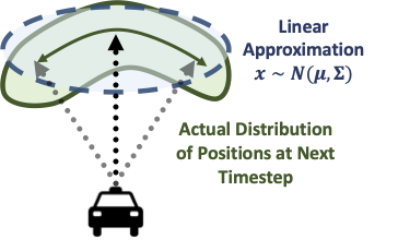
When representing this formulation in terms of Gaussian parameters, we point out that the functions and applied on Gaussian random variables do not produce Gaussians:
To amend this, we instead replace and with linear approximations evaluated at .
We now derive the formulation of the distribution of positions with the linear approximations instead:
where
| (5) | ||||
| (6) | ||||
| (7) | ||||
| (8) | ||||
| (9) |
and
| (10) | ||||
| (11) | ||||
| (12) | ||||
| (13) | ||||
| (14) |
The full expansion of these terms is described in Section VII-A of the appendix, which can be found on our project page under the title.
IV-B4 Formulation 4: Acceleration and Steering
Lastly, we derive a second-order kinematic formulation based on the bicycle model: steering and acceleration . This formulation is the second-order version of the velocity-heading formulation. Here, we assume acceleration to be scalar and directionless, in contrast to Formulation 2, where we consider acceleration to be a vector with lateral and longitudinal components. Similarly to Formulation 2, we also use the linear approximation of in order to derive approximated position distributions.
Following the Bicycle Model, the update for speed and heading at each timestep is:
Where is the length of the agent. When we represent this process probabilistically as random Gaussian variables, we solve for the distributions of first-order variables, speed () and heading ():
where
| (15) | ||||
| (16) | ||||
| (17) | ||||
| (18) | ||||
| (19) | ||||
| (20) | ||||
| (21) |
With the computed distributions of speed and heading, we can then use the analytical definitions from Formulation 3, in Equation 5, to derive the distribution of positions in terms of and .
IV-C Error Bound of Linear Approximation.
The linear approximations used to derive the variance in predicted trajectories come with some error relative to the actual variance computed from transformations on predicted Gaussian variables, which may not necessarily be easily computable or known. However, we can bound the error of this linear approximation thanks to the alternating property of the sine and cosine Taylor expansions.
We analytically derive the error bound for the linear approximation for and functions at . Since the Taylor series expansion of both functions are alternating, the error is bounded by the term representing the second order derivative:
For both functions, the Lagrange error is bounded by .
In other words, the error from each linear approximation is, at most, on the order of , where is a random variable sampled from . While this error can compound across timesteps, we point out that values empirically remain quite small within the task (bounded most of the time by road width or differences in speed), where one unit value is one meter, as well as the random chi-square variable being heavily biased towards 0 ( probability under 1, and probability under 4 for normal chi-square distribution).
V Results
In this section, we show experiments that highlight the effect of kinematic priors on performance. We implement kinematic priors on state-of-the-art method Motion Transformer (MTR) [13], which serves as our baseline method.
Hardware. We train all experiments on eight RTX A5000 GPUs, with 64 GB of memory and 32 CPU cores. Experiments on the full dataset are trained for 30 epochs, while experiments with the smaller dataset are trained for 50 epochs. Additionally, we downscale the model from its original size of 65 million parameters to 2 million parameters and re-train all models under these settings for fair comparison. Furthermore, we re-implement Deep Kinematic Models (DKM) [3] to contextualize our probabilistic method against deterministic methods, as the official implementation is not publicly available. DKM is implemented against the same backbone as vanilla MTR and our models. More details on training hyperparameters can be found in Table VIII of the appendix, which can also be found on the project website.
| Method | mAP | minADE | minFDE | MissRate |
|---|---|---|---|---|
| MTR | 0.3872 | 0.8131 | 1.6700 | 0.1817 |
| DKM | 0.3613 | 0.8724 | 1.7685 | 0.1994 |
| Ours + Formulation 1 | 0.3880 | 0.8241 | 1.6783 | 0.1834 |
| Ours + Formulation 2 | 0.3892 | 0.8217 | 1.6710 | 0.1829 |
| Ours + Formulation 3 | 0.3914 | 0.8102 | 1.6634 | 0.1792 |
| Ours + Formulation 4 | 0.3910 | 0.8220 | 1.6782 | 0.1830 |
V-A Performance on Waymo Motion Prediction Dataset
We evaluate the baseline model and all kinematic formulations on the Waymo Motion Prediction Dataset [9]. The Waymo dataset consists of over 100,000 segments of traffic, where each scenario contains multiple agents of three classes: vehicles, pedestrians, and cyclists. The data is collected from high-quality, high-resolution sensors that sample traffic states at 10 Hz. The objective is, given 1 second of trajectory history for each vehicle, to predict trajectories for the next 8 seconds. For simplicity, we use the bicycle kinematic model for all three classes and leave discerning between the three, especially for pedestrians, for future work.
We evaluate our model’s performance on Mean Average Precision (mAP), Minimum Average Displacement Error (minADE), minimum final displacement error (minFDE), and Miss Rate, similarly to [9]. We reiterate their definitions below for convenience.
-
•
Mean Average Precision (mAP): mAP is computed across all classes of trajectories. The classes include straight, straight-left, straight-right, left, right, left u-turn, right u-turn, and stationary. For each prediction, one true positive is chosen based on the highest confidence trajectory within a defined threshold of the ground truth trajectory, while all other predictions are assigned a false positive. Intuitively, the mAP metric describes prediction precision while accounting for all trajectory class types. This is beneficial especially when there is an imbalance of classes in the dataset (e.g., there may be many more straight-line trajectories in the dataset than there are right u-turns).
-
•
Minimum Average Displacement Error (minADE): The average L2 norm between the ground truth and the closest prediction; .
-
•
Minimum final displacement error (minFDE): The L2 norm between only the positions at the final timestep, ; .
-
•
Miss Rate: The number of predictions lying outside a reasonable threshold from the ground truth. The miss rate first describes the ratio of object predictions lying outside a threshold from the ground truth to the total number of agents predicted.
We show results for the Waymo Motion dataset in Table I, where we compared performance across two baselines, MTR [13] and DKM [3], and all formulations. From these results, we observe the greatest improvement over the baseline with Formulation 3, which involves the first-order velocity and heading components. We observe that the benefit of our method in full-scale training settings diminishes. This performance gap closing may be due to the computational complexity of the network, the large dataset, and or the long supervised training time out-scaling benefits provided by applying kinematic constraints. However, deploying models in the wild may not necessarily have such optimal settings, especially in cases of sparse data or domain transfer. Thus, we also consider the effects of suboptimal settings for trajectory prediction, as we hypothesize that learning first or second-order terms provides information when data cannot. This is also motivated by problems in the real world, where sensors may not be as high-quality or specific traffic scenarios may not be so abundantly represented in data.
| Method | mAP | minADE | minFDE | MissRate |
|---|---|---|---|---|
| MTR | 0.1697 | 1.4735 | 3.7602 | 0.3723 |
| DKM | 0.1283 | 1.6632 | 3.7148 | 0.4361 |
| Ours + Formulation 1 | 0.1920 | 1.3053 | 2.7907 | 0.3501 |
| Ours + Formulation 2 | 0.1860 | 1.4386 | 2.7788 | 0.3500 |
| Ours + Formulation 3 | 0.1856 | 1.3322 | 2.7717 | 0.3470 |
| Ours + Formulation 4 | 0.1846 | 1.2948 | 2.8291 | 0.3541 |
V-B Performance on a Smaller Dataset Setting
We examine the effects of kinematic priors on a smaller dataset size. This is motivated by the fact driving datasets naturally have an imbalance of scenarios, where many samples are representative of longitudinal straight-line driving or stationary movement, and much less are representative of extreme lateral movements such as U-turns. Thus, large and robust benchmarks like the Waymo, Nuscenes, and Argoverse datasets are necessary for learning good models.
However, large datasets are not always accessible depending on the setting. For example, traffic laws, road design, and natural dynamics vary by region. It would be infeasible to expect the same scale and robustness of data from every scenario in the world, and thus trajectory forecasting will run into settings with less data available.
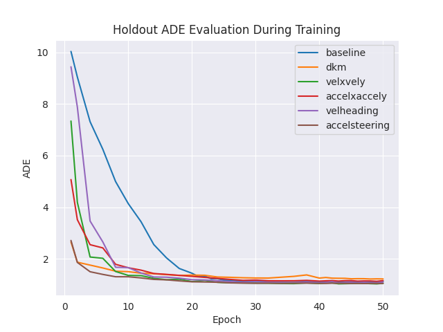
We train the baseline model and all formulations on only 1% of the original Waymo dataset and benchmark their performance on 100% of the evaluation set in Table II. All experiments were trained over 50 epochs. In the small dataset setting, we observe that providing a kinematic prior in any form improves performance for minimum final displacement error (minFDE). Additionally, we observe better performance across all metrics for formulations 1, 2, and 1 with interpolation. Figure 4 shows how all kinematic formulations improve convergence speed over the baseline, with Formulation 4 (acceleration and steering) converging most quickly. Overall, Formulation 1 provides the greatest boost in mAP performance, with over gain over the vanilla baseline and over the deterministic baseline DKM. Additionally, Formulation 4 provides a reduction in minADE, while Formulation 3 provides a reduction in minFDE and a reduction in Miss Rate. In general, all formulations provide similar benefits in the small dataset setting, with the most general performance benefit coming from Formulation 3. While Formulation 4 also provides a comparable performance boost, the difference from Formulation 3 may be attributed to compounding error from second-order approximation.
Compared to the results from Table I, the effects of kinematic priors in learning are much more pronounced. Since kinematic priors naturally relate the position at one timestep to the position at the next, we believe that the performance boost can be attributed to this natural relationship. In backpropagation, optimization of one position further into the time horizon directly influences predicted positions at earlier timesteps via the kinematic model. Without the kinematic prior, the relation between timesteps may be implicitly related through neural network parameters. When the model lacks data to form a good model of how an agent moves through space, the kinematic model can compensate to model such simple relationships.
V-C Performance in the Presence of Noise
We also show how kinematic priors can influence performance in the presence of noise. This is inspired by the scenario where sensors may have a small degree of noise associated with measurements dependent on various factors, such as weather, quality, interference, etc.
We evaluate the models from Table III when input trajectories are perturbed by standard normal noise ; results for performance degradation are shown in Table III.
We compute results in Table III by measuring the % of degradation of the perturbed evaluation from the corresponding original clean evaluation. We find that Formulation 4 from Section IV-B4 with steering and acceleration components preserves the most performance in the presence of noise. This may be due to that second-order terms like acceleration are less influenced by perturbations on position, in addition to providing explicit bicycle-like constraints on vehicle movement. Additionally, distributions of acceleration are typically centered around zero regardless of how positions are distributed [35], which may provide more stability for learning.
| Method | mAP | minADE | minFDE | MissRate |
|---|---|---|---|---|
| MTR | -2.965 | 2.302 | 0.671 | 1.928 |
| Ours + Formulation 1 | -5.271 | 1.436 | 0.710 | 1.849 |
| Ours + Formulation 2 | -5.780 | 1.809 | 0.897 | 2.475 |
| Ours + Formulation 3 | -3.445 | 1.052 | 0.369 | 1.510 |
| Ours + Formulation 4 | -2.028 | 1.165 | 1.375 | 0.823 |
VI Discussion and Conclusion
In this paper, we present a simple and easy-to-implement method for including kinematic priors in probabilistic trajectory forecasting. Kinematic priors can also be implemented for deterministic methods where linear approximations are not necessary. With no additional overhead, kinematic priors not only show improvement in models trained on robust datasets but also in suboptimal settings with small datasets and noisy trajectories, with up to improvement in smaller datasets and less performance degradation in the presence of noise for the full Waymo dataset. For overall performance improvement, we find Formulation 1 in Section IV-B1 with velocity components to be the most beneficial and well-rounded to prediction performance.
We also observe that when there is large-scale data to learn a good model of how vehicles move, the effects of kinematic priors are less pronounced. This can be observed from the less obvious improvements over the baseline in Table I compared to Table II. We conjecture that model complexity and dataset size will eventually out-scale the effects of the kinematic prior. With enough resources and high-quality data, trajectory forecasting models will learn to “reinvent the steering wheel”, or implicitly learn how vehicles move via the complexity of the neural network. For practical autonomous systems, portability and adaptability are important problems to consider aside into the future. We hope that kinematic priors can be considered in trajectory forecasting and simulation as deployment ventures past well-represented urban scenarios to suboptimal settings, whether it is with noisy sensors, smaller datasets to adapt from, or downscaled models for inference speed and portability.
In future work, kinematic priors can be further explored for transfer learning between domains. While distributions of trajectories may change in scale and distribution depending on the environment, kinematic parameters, especially on the second order, will remain more constant between domains.
References
- [1] M. Bojarski, D. Del Testa, D. Dworakowski, B. Firner, B. Flepp, P. Goyal, L. D. Jackel, M. Monfort, U. Muller, J. Zhang, et al., “End to end learning for self-driving cars,” arXiv preprint arXiv:1604.07316, 2016.
- [2] K. Chitta, A. Prakash, B. Jaeger, Z. Yu, K. Renz, and A. Geiger, “Transfuser: Imitation with transformer-based sensor fusion for autonomous driving,” Pattern Analysis and Machine Intelligence (PAMI), 2022.
- [3] H. Cui, T. Nguyen, F.-C. Chou, T.-H. Lin, J. Schneider, D. Bradley, and N. Djuric, “Deep kinematic models for kinematically feasible vehicle trajectory predictions,” in 2020 IEEE International Conference on Robotics and Automation (ICRA), p. 10563–10569, IEEE, May 2020.
- [4] C. Anderson, R. Vasudevan, and M. Johnson-Roberson, “A kinematic model for trajectory prediction in general highway scenarios,” IEEE Robotics and Automation Letters, vol. 6, p. 6757–6764, Oct 2021.
- [5] S. Suo, K. Wong, J. Xu, J. Tu, A. Cui, S. Casas, and R. Urtasun, “Mixsim: A hierarchical framework for mixed reality traffic simulation,” in 2023 IEEE/CVF Conference on Computer Vision and Pattern Recognition (CVPR), p. 9622–9631, IEEE, Jun 2023.
- [6] B. Varadarajan, A. Hefny, A. Srivastava, K. S. Refaat, N. Nayakanti, A. Cornman, K. Chen, B. Douillard, C. P. Lam, D. Anguelov, et al., “Multipath++: Efficient information fusion and trajectory aggregation for behavior prediction,” in 2022 International Conference on Robotics and Automation (ICRA), pp. 7814–7821, IEEE, 2022.
- [7] F. Farahi and H. S. Yazdi, “Probabilistic kalman filter for moving object tracking,” Signal Processing: Image Communication, vol. 82, p. 115751, 2020.
- [8] C. G. Prevost, A. Desbiens, and E. Gagnon, “Extended kalman filter for state estimation and trajectory prediction of a moving object detected by an unmanned aerial vehicle,” in 2007 American Control Conference, p. 1805–1810, IEEE, July 2007.
- [9] S. Ettinger, S. Cheng, B. Caine, C. Liu, H. Zhao, S. Pradhan, Y. Chai, B. Sapp, C. R. Qi, Y. Zhou, Z. Yang, A. Chouard, P. Sun, J. Ngiam, V. Vasudevan, A. McCauley, J. Shlens, and D. Anguelov, “Large scale interactive motion forecasting for autonomous driving: The waymo open motion dataset,” in Proceedings of the IEEE/CVF International Conference on Computer Vision (ICCV), pp. 9710–9719, October 2021.
- [10] K. Chen, R. Ge, H. Qiu, R. Ai-Rfou, C. R. Qi, X. Zhou, Z. Yang, S. Ettinger, P. Sun, Z. Leng, M. Mustafa, I. Bogun, W. Wang, M. Tan, and D. Anguelov, “Womd-lidar: Raw sensor dataset benchmark for motion forecasting,” arXiv preprint arXiv:2304.03834, April 2023.
- [11] B. Wilson, W. Qi, T. Agarwal, J. Lambert, J. Singh, S. Khandelwal, B. Pan, R. Kumar, A. Hartnett, J. Kaesemodel Pontes, D. Ramanan, P. Carr, and J. Hays, “Argoverse 2: Next generation datasets for self-driving perception and forecasting,” in Proceedings of the Neural Information Processing Systems Track on Datasets and Benchmarks (J. Vanschoren and S. Yeung, eds.), vol. 1, Curran, 2021.
- [12] H. Caesar, V. Bankiti, A. H. Lang, S. Vora, V. E. Liong, Q. Xu, A. Krishnan, Y. Pan, G. Baldan, and O. Beijbom, “nuscenes: A multimodal dataset for autonomous driving,” in CVPR, 2020.
- [13] S. Shi, L. Jiang, D. Dai, and B. Schiele, “Motion transformer with global intention localization and local movement refinement,” Advances in Neural Information Processing Systems, 2022.
- [14] C. Qian, D. Xiu, and M. Tian, “The 2nd place solution for 2023 waymo open sim agents challenge,” 2023.
- [15] Y. Liu, J. Zhang, L. Fang, Q. Jiang, and B. Zhou, “Multimodal motion prediction with stacked transformers,” Computer Vision and Pattern Recognition, 2021.
- [16] Z. Zhou, J. Wang, Y.-H. Li, and Y.-K. Huang, “Query-centric trajectory prediction,” in Proceedings of the IEEE/CVF Conference on Computer Vision and Pattern Recognition (CVPR), 2023.
- [17] J. Ngiam, V. Vasudevan, B. Caine, Z. Zhang, H.-T. L. Chiang, J. Ling, R. Roelofs, A. Bewley, C. Liu, A. Venugopal, et al., “Scene transformer: A unified architecture for predicting future trajectories of multiple agents,” in International Conference on Learning Representations, 2021.
- [18] Y. Chai, B. Sapp, M. Bansal, and D. Anguelov, “Multipath: Multiple probabilistic anchor trajectory hypotheses for behavior prediction,” in Proceedings of the Conference on Robot Learning (L. P. Kaelbling, D. Kragic, and K. Sugiura, eds.), vol. 100 of Proceedings of Machine Learning Research, pp. 86–99, PMLR, 30 Oct–01 Nov 2020.
- [19] A. Ścibior, V. Lioutas, D. Reda, P. Bateni, and F. Wood, “Imagining the road ahead: Multi-agent trajectory prediction via differentiable simulation,” in 2021 IEEE International Intelligent Transportation Systems Conference (ITSC), p. 720–725, IEEE, Sep 2021.
- [20] D. Rempe, J. Philion, L. J. Guibas, S. Fidler, and O. Litany, “Generating useful accident-prone driving scenarios via a learned traffic prior,” in Conference on Computer Vision and Pattern Recognition (CVPR), 2022.
- [21] M. Lutter, C. Ritter, and J. Peters, “Deep lagrangian networks: Using physics as model prior for deep learning,” in International Conference on Learning Representations (ICLR), 2019.
- [22] S. Greydanus, M. Dzamba, and J. Yosinski, “Hamiltonian neural networks,” in Advances in Neural Information Processing Systems (H. Wallach, H. Larochelle, A. Beygelzimer, F. d'Alché-Buc, E. Fox, and R. Garnett, eds.), vol. 32, Curran Associates, Inc., 2019.
- [23] M. Janner, J. Fu, M. Zhang, and S. Levine, “When to trust your model: Model-based policy optimization,” in Advances in Neural Information Processing Systems, 2019.
- [24] F. de Avila Belbute-Peres, K. Smith, K. Allen, J. Tenenbaum, and J. Z. Kolter, “End-to-end differentiable physics for learning and control,” Advances in neural information processing systems, vol. 31, 2018.
- [25] J. Degrave, M. Hermans, J. Dambre, et al., “A differentiable physics engine for deep learning in robotics,” Frontiers in neurorobotics, p. 6, 2019.
- [26] M. Geilinger, D. Hahn, J. Zehnder, M. Bächer, B. Thomaszewski, and S. Coros, “Add: Analytically differentiable dynamics for multi-body systems with frictional contact,” ACM Transactions on Graphics (TOG), vol. 39, no. 6, pp. 1–15, 2020.
- [27] Y.-L. Qiao, J. Liang, V. Koltun, and M. C. Lin, “Scalable differentiable physics for learning and control,” in ICML, 2020.
- [28] S. Son, L. Zheng, R. Sullivan, Y. Qiao, and M. Lin, “Gradient informed proximal policy optimization,” in Advances in Neural Information Processing Systems, 2023.
- [29] J. Xu, V. Makoviychuk, Y. Narang, F. Ramos, W. Matusik, A. Garg, and M. Macklin, “Accelerated policy learning with parallel differentiable simulation,” in International Conference on Learning Representations, 2021.
- [30] J. Liang, M. Lin, and V. Koltun, “Differentiable cloth simulation for inverse problems,” Advances in Neural Information Processing Systems, vol. 32, 2019.
- [31] Y. Chai, B. Sapp, M. Bansal, and D. Anguelov, “Multipath: Multiple probabilistic anchor trajectory hypotheses for behavior prediction,” in Proceedings of the Conference on Robot Learning (L. P. Kaelbling, D. Kragic, and K. Sugiura, eds.), vol. 100 of Proceedings of Machine Learning Research, pp. 86–99, PMLR, 30 Oct–01 Nov 2020.
- [32] B. Varadarajan, A. Hefny, A. Srivastava, K. S. Refaat, N. Nayakanti, A. Cornman, K. Chen, B. Douillard, C. P. Lam, D. Anguelov, and B. Sapp, “Multipath++: Efficient information fusion and trajectory aggregation for behavior prediction,” in 2022 International Conference on Robotics and Automation (ICRA), p. 7814–7821, IEEE Press, 2022.
- [33] Y. Wang, T. Zhao, and F. Yi, “Multiverse transformer: 1st place solution for waymo open sim agents challenge 2023,” arXiv preprint arXiv:2306.11868, 2023.
- [34] D. P. Kingma and M. Welling, “Auto-encoding variational bayes,” 2022.
- [35] B. M. Albaba and Y. Yildiz, “Driver modeling through deep reinforcement learning and behavioral game theory,” IEEE Transactions on Control Systems Technology, vol. 30, no. 2, pp. 885–892, 2022.
VII Appendix
VII-A Full Expansion of Formulation 3
VII-B Additional Results By Class
In the paper, we present results on vehicles since we use kinematic models based on vehicles as priors. Here, we present the full results per-class for each experiment in Tables IV, V, VI, and VII. The results reported in the paper are starred (*), which are re-iterated below for full context.
| Class | Method | mAP | minADE | minFDE | MissRate |
|---|---|---|---|---|---|
| Average | Baseline | 0 | 0 | 0 | 0 |
| Ours + Formulation 1 | 1.7492 | -0.4455 | -2.3882 | -1.1098 | |
| Ours + Formulation 2 | -2.2235 | 0.1337 | -1.0881 | -0.7009 | |
| Ours + Formulation 3 | -0.9487 | -0.4604 | -0.7560 | 1.2850 | |
| Ours + Formulation 1 + Interpolation | -0.5336 | 1.4553 | -1.6534 | 0.0000 | |
| Vehicle* | Baseline | 0 | 0 | 0 | 0 |
| Ours + Formulation 1 | 2.376 | -0.3444 | -0.9102 | -0.3853 | |
| Ours + Formulation 2 | -0.2066 | 1.1069 | 0.1138 | -0.1651 | |
| Ours + Formulation 3 | -1.7045 | 0.246 | 1.0838 | 3.1921 | |
| Ours + Formulation 1 + Interpolation | 0.9039 | 2.2260 | -0.7365 | -0.4403 | |
| Pedestrian | Baseline | 0 | 0 | 0 | 0 |
| Ours + Formulation 1 | 0.4657 | 0.2343 | -0.7773 | -2.7692 | |
| Ours + Formulation 2 | -1.2806 | 0.885 | -0.2065 | -3.8974 | |
| Ours + Formulation 3 | 0.0873 | 0.9630 | 0.6072 | -1.9487 | |
| Ours + Formulation 1 + Interpolation | 0.3492 | 4.1385 | 1.4574 | 0.8205 | |
| Cyclist | Baseline | 0 | 0 | 0 | 0 |
| Ours + Formulation 1 | 2.4911 | -0.8991 | -4.5646 | -1.0656 | |
| Ours + Formulation 2 | -6.0854 | -1.1786 | -2.6418 | 0.1279 | |
| Ours + Formulation 3 | -1.2100 | -1.8348 | -3.1439 | 1.0230 | |
| Ours + Formulation 1 + Interpolation | -3.5943 | -0.5832 | -3.9884 | 0.0000 |
| Class | Method | mAP | minADE | minFDE | MissRate |
|---|---|---|---|---|---|
| Average | Baseline | 0 | 0 | 0 | 0 |
| Ours + Formulation 1 | -1.6418 | -6.3763 | -14.9755 | -5.173 | |
| Ours + Formulation 2 | 0.7463 | -0.7756 | -14.5275 | -2.9916 | |
| Ours + Formulation 3 | -6.1692 | 16.0354 | -11.2498 | -0.2493 | |
| Ours + Formulation 1 + Interpolation | -1.2438 | -2.1014 | -12.2530 | -0.0312 | |
| Vehicle* | Baseline | 0 | 0 | 0 | 0 |
| Ours + Formulation 1 | 11.8444 | -12.5280 | -27.1767 | -8.3266 | |
| Ours + Formulation 2 | 6.7767 | -5.8432 | -27.7645 | -7.2791 | |
| Ours + Formulation 3 | -5.3035 | 30.6413 | -20.5494 | -0.8327 | |
| Ours + Formulation 1 + Interpolation | 4.1839 | -7.3498 | -23.8817 | -4.8080 | |
| Pedestrian | Baseline | 0 | 0 | 0 | 0 |
| Ours + Formulation 1 | -7.8373 | -1.1325 | -1.2123 | 3.2820 | |
| Ours + Formulation 2 | -11.1275 | 1.7743 | -0.9999 | 6.2960 | |
| Ours + Formulation 3 | -3.2902 | -0.6795 | -3.0440 | 0.1340 | |
| Ours + Formulation 1 + Interpolation | -8.0961 | 3.7750 | 1.3716 | 11.2525 | |
| Cyclist | Baseline | 0 | 0 | 0 | 0 |
| Ours + Formulation 1 | -5.5283 | -1.6251 | -4.6731 | -5.3754 | |
| Ours + Formulation 2 | 14.2506 | 3.8549 | -2.8120 | -2.4949 | |
| Ours + Formulation 3 | -11.9165 | 6.4701 | -2.5166 | 0.1588 | |
| Ours + Formulation 1 + Interpolation | 4.4840 | 1.3908 | -2.6320 | 0.2041 |
| Class | Method | mAP | minADE | minFDE | MissRate |
|---|---|---|---|---|---|
| Average | Baseline | -2.5793 | 2.5097 | 0.7066 | 1.6939 |
| Ours + Formulation 1 | -2.9138 | 1.5662 | 0.3547 | -0.6497 | |
| Ours + Formulation 2 | -3.2141 | 1.4385 | 0.9715 | 1.8824 | |
| Ours + Formulation 3 | -3.5917 | 1.7306 | 0.7760 | 0.6344 | |
| Vehicle* | Baseline | -4.9587 | 4.7965 | 1.6527 | 3.5223 |
| Ours + Formulation 1 | -4.9445 | 3.5542 | 1.4322 | 2.7072 | |
| Ours + Formulation 2 | -3.9596 | 2.4693 | 1.2800 | 2.7012 | |
| Ours + Formulation 3 | -4.7294 | 3.3984 | 1.3447 | 2.5600 | |
| Pedestrian | Baseline | -1.1932 | 0.8329 | 0.0243 | 3.3846 |
| Ours + Formulation 1 | -1.5933 | -0.2077 | -0.7344 | -1.0549 | |
| Ours + Formulation 2 | -3.066 | 0.4902 | 0.1582 | 2.7748 | |
| Ours + Formulation 3 | -2.0646 | 0.4383 | 0.4587 | 2.7197 | |
| Cyclist | Baseline | -0.9253 | 1.0207 | 0.1255 | -0.5541 |
| Ours + Formulation 1 | -1.6667 | 0.4537 | -0.1614 | -3.0590 | |
| Ours + Formulation 2 | -2.3494 | 0.8361 | 1.0608 | 0.9366 | |
| Ours + Formulation 3 | -3.8905 | 0.6560 | 0.3594 | -1.7300 |
| Class | Method | mAP | minADE | minFDE | MissRate |
|---|---|---|---|---|---|
| Average | Baseline | -3.4328 | 0.5411 | 0.1187 | 0.1246 |
| Ours + Formulation 1 | -6.2721 | 0.1349 | -0.1171 | 0.6901 | |
| Ours + Formulation 2 | -3.3086 | 0.7635 | 0.3181 | 1.574 | |
| Ours + Formulation 3 | -4.0297 | 0.3420 | 0.8672 | 2.2805 | |
| Vehicle | Baseline | -6.0695 | 1.1266 | 0.2207 | 0.9132 |
| Ours + Formulation 1 | -4.4784 | 1.0241 | 0.8180 | 1.2892 | |
| Ours + Formulation 2 | -5.6843 | 1.8236 | 1.3033 | 1.5933 | |
| Ours + Formulation 3 | -5.6005 | -0.3117 | 0.4686 | 0.4605 | |
| Pedestrian | Baseline | -0.2957 | -1.1136 | -0.9734 | -2.6122 |
| Ours + Formulation 1 | -4.4124 | -0.3627 | -0.8599 | -0.0649 | |
| Ours + Formulation 2 | -3.0782 | -0.2411 | -0.3396 | 2.8355 | |
| Ours + Formulation 3 | -4.8930 | -0.3421 | -0.2008 | 2.9431 | |
| Cyclist | Baseline | -5.8354 | 0.5518 | 0.4041 | 0.4083 |
| Ours + Formulation 1 | -11.3134 | -0.5455 | -0.7410 | 0.5273 | |
| Ours + Formulation 2 | -1.3978 | 0.1019 | -0.3669 | 1.1398 | |
| Ours + Formulation 3 | -0.6276 | 1.4908 | 1.6792 | 3.5779 |
VII-C Experiment Hyperparameters
| Component | Hyperparameter | Value |
| Encoder | # Hidden Features | 128 |
| # Attention Layers | 2 | |
| # Attention Heads | 2 | |
| Local Attention | True | |
| Decoder | Hidden Features | 128 |
| # Decoder Layers | 2 | |
| # Attention Heads | 2 | |
| # Hidden Map Features | 64 |