DESY-24-070 \prepdateMay 2024
3.5
The azimuthal correlation between the leading jet and the scattered lepton in deep inelastic scattering at HERA
ZEUS Collaboration
Abstract
The azimuthal correlation angle, , between the scattered lepton and the leading jet in deep inelastic scattering at HERA has been studied using data collected with the ZEUS detector at a centre-of-mass energy of , corresponding to an integrated luminosity of . A measurement of jet cross sections in the laboratory frame was made in a fiducial region corresponding to photon virtuality , inelasticity , outgoing lepton energy , lepton polar angle , jet transverse momentum , and jet pseudorapidity . Jets were reconstructed using the algorithm with the radius parameter . The leading jet in an event is defined as the jet that carries the highest . Differential cross sections, , were measured as a function of the azimuthal correlation angle in various ranges of leading-jet transverse momentum, photon virtuality and jet multiplicity. Perturbative calculations at accuracy successfully describe the data within the fiducial region, although a lower level of agreement is observed near for events with high jet multiplicity, due to limitations of the perturbative approach in describing soft phenomena in QCD. The data are equally well described by Monte Carlo predictions that supplement leading-order matrix elements with parton showering.
The ZEUS Collaboration
I. Abt1, R. Aggarwal2, V. Aushev3, O. Behnke4, A. Bertolin5, I. Bloch6, I. Brock7, N.H. Brook8,a, R. Brugnera9, A. Bruni10, P.J. Bussey11, A. Caldwell1, C.D. Catterall12, J. Chwastowski13, J. Ciborowski14,b, R. Ciesielski4,c, A.M. Cooper-Sarkar15, M. Corradi10,d, R.K. Dementiev16, S. Dusini5, J. Ferrando17, B. Foster15,e, E. Gallo18,f, D. Gangadharan19,g, A. Garfagnini9, A. Geiser4, G. Grzelak14, C. Gwenlan15, D. Hochman20, N.Z. Jomhari4, I. Kadenko3, U. Karshon20, P. Kaur21, R. Klanner18, U. Klein4,h, I.A. Korzhavina16, N. Kovalchuk18, M. Kuze22, B.B. Levchenko16, A. Levy23, B. Löhr4, E. Lohrmann18, A. Longhin9, F. Lorkowski24, E. Lunghi25, I. Makarenko4, J. Malka4,i, S. Masciocchi26,j, K. Nagano27, J.D. Nam28, Yu. Onishchuk3, E. Paul7, I. Pidhurskyi29, A. Polini10, M. Przybycień30, A. Quintero28, M. Ruspa31, U. Schneekloth4, T. Schörner-Sadenius4, I. Selyuzhenkov26, M. Shchedrolosiev4, L.M. Shcheglova16, N. Sherrill32, I.O. Skillicorn11, W. Słomiński33, A. Solano34, L. Stanco5, N. Stefaniuk4, B. Surrow28, K. Tokushuku27, O. Turkot4,i, T. Tymieniecka35, A. Verbytskyi1, W.A.T. Wan Abdullah36, K. Wichmann4, M. Wing8,k, S. Yamada27, Y. Yamazaki37, A.F. Żarnecki14, O. Zenaiev4,l
1 Max-Planck-Institut für Physik, München, Germany
2 DST-Inspire Faculty, Department of Technology, SPPU, India
3 Department of Nuclear Physics, National Taras Shevchenko University of Kyiv, Kyiv, Ukraine
4 Deutsches Elektronen-Synchrotron DESY, Hamburg, Germany
5 INFN Padova, Padova, Italy A
6 Deutsches Elektronen-Synchrotron DESY, Zeuthen, Germany
7 Physikalisches Institut der Universität Bonn, Bonn, Germany B
8 Physics and Astronomy Department, University College London, London, United Kingdom C
9 Dipartimento di Fisica e Astronomia dell’ Università and INFN, Padova, Italy A
10 INFN Bologna, Bologna, Italy A
11 School of Physics and Astronomy, University of Glasgow, Glasgow, United Kingdom C
12 Department of Physics, York University, Ontario, Canada M3J 1P3 D
13 The Henryk Niewodniczanski Institute of Nuclear Physics, Polish Academy of Sciences, Krakow, Poland
14 Faculty of Physics, University of Warsaw, Warsaw, Poland
15 Department of Physics, University of Oxford, Oxford, United Kingdom C
16 Affiliated with an institute covered by a current or former collaboration agreement with DESY
17 Physics Department, Lancaster University, Lancaster, United Kingdom
18 Hamburg University, Institute of Experimental Physics, Hamburg, Germany E
19 Physikalisches Institut of the University of Heidelberg, Heidelberg, Germany
20 Department of Particle Physics and Astrophysics, Weizmann Institute, Rehovot, Israel
21 Sant Longowal Institute of Engineering and Technology, Longowal, Punjab, India
22 Department of Physics, Tokyo Institute of Technology, Tokyo, Japan F
23 Raymond and Beverly Sackler Faculty of Exact Sciences, School of Physics, Tel Aviv University, Tel Aviv, Israel G
24 Physik-Institut, University of Zurich, Zurich, Switzerland
25 Department of Physics, Indiana University Bloomington, Bloomington, IN 47405, USA
26 GSI Helmholtzzentrum für Schwerionenforschung GmbH, Darmstadt, Germany
27 Institute of Particle and Nuclear Studies, KEK, Tsukuba, Japan F
28 Department of Physics, Temple University, Philadelphia, PA 19122, USA H
29 Institut für Kernphysik, Goethe Universität, Frankfurt am Main, Germany
30 AGH University of Science and Technology, Faculty of Physics and Applied Computer Science, Krakow, Poland
31 Università del Piemonte Orientale, Novara, and INFN, Torino, Italy A
32 Department of Physics and Astronomy, University of Sussex, Brighton, BN1 9QH, United Kingdom I
33 Department of Physics, Jagellonian University, Krakow, Poland J
34 Università di Torino and INFN, Torino, Italy A
35 National Centre for Nuclear Research, Warsaw, Poland
36 National Centre for Particle Physics, Universiti Malaya, 50603 Kuala Lumpur, Malaysia K
37 Department of Physics, Kobe University, Kobe, Japan F
A supported by the Italian National Institute for Nuclear Physics (INFN)
B supported by the German Federal Ministry for Education and Research (BMBF), under contract No. 05 H09PDF
C supported by the Science and Technology Facilities Council, UK
D supported by the Natural Sciences and Engineering Research Council of Canada (NSERC)
E supported by the German Federal Ministry for Education and Research (BMBF), under contract No. 05h09GUF, and the SFB 676 of the Deutsche Forschungsgemeinschaft (DFG)
F supported by the Japanese Ministry of Education, Culture, Sports, Science and Technology (MEXT) and its grants for Scientific Research
G supported by the Israel Science Foundation
H supported in part by the Office of Nuclear Physics within the U.S. DOE Office of Science
I supported in part by the Science and Technology Facilities Council grant number ST/T006048/1
J supported by the Polish National Science Centre (NCN) grant no. DEC-2014/13/B/ST2/02486
K supported by HIR grant UM.C/625/1/HIR/149 and UMRG grants RU006-2013, RP012A-13AFR and RP012B-13AFR from Universiti Malaya, and ERGS grant ER004-2012A from the Ministry of Education, Malaysia
a now at University of Bath, United Kingdom
b also at Lodz University, Poland
c now at Rockefeller University, New York, NY 10065, USA
d now at INFN Roma, Italy
e also at DESY and University of Hamburg, Hamburg, Germany and supported by a Leverhulme Trust Emeritus Fellowship
f also at DESY, Hamburg, Germany
g now at University of Houston, Houston, TX 77004, USA
h now at University of Liverpool, United Kingdom
i now at European X-ray Free-Electron Laser facility GmbH, Hamburg, Germany
j also at Physikalisches Institut of the University of Heidelberg, Heidelberg, Germany
k also supported by DESY, Hamburg, Germany
l now at Hamburg University, II. Institute for Theoretical Physics, Hamburg, Germany
1 Introduction
The HERA collider provided events111In this paper, both electrons and positrons are referred to as electrons. that are a unique basis for tests of a wide range of predictions based on perturbative Quantum Chromodynamics (pQCD). Jet production at HERA continues to be used for rigorous tests of the validity of pQCD [1, 2]. The azimuthal distribution of jets with respect to the outgoing lepton in deep inelastic scattering (DIS) provides an interesting means of investigating both soft and hard phenomena in QCD, and is the subject of the present paper. In neutral current (NC) DIS mediated by a virtual boson, a final-state jet can be produced at the Born limit () of DIS via the following process:
| (1) |
The azimuthal correlation angle, , is defined as the difference in the azimuthal angle between the scattered lepton, , and the final-state jet, , where all quantities are specified in the laboratory frame. The lepton–jet pairs in reaction (1) are produced in a back-to-back topology, . Small deviations from the back-to-back topology arise if soft gluons are emitted and/or if the struck parton carries a non-zero transverse momentum [3, 4]. Larger deviations from are expected when additional jets are produced through hard gluon radiation. This sensitivity to various QCD phenomena, including both soft and hard processes, allows evaluation of theoretical models without explicitly describing the additional jets arising from higher-order (, ) processes.
Azimuthal correlations in photoproduction have been studied by the ZEUS collaboration for various final-state systems [5, 6, 7] to test the validity of perturbative QCD predictions. Measurements of azimuthal correlations in multijet systems in hadron collisions have been performed by the D experiment at the Tevatron [8], as well as by the CMS [9, 10, 11] and ATLAS [12, 13] experiments at the LHC, in order to investigate the effects of soft and hard QCD radiation in the high-energy regime. The H1 collaboration recently published [14] a measurement of the azimuthal correlation between the DIS scattered lepton and jets in the event. The azimuthal correlation in dijet production in transversely polarised hadron collisions has been measured by the STAR experiment at RHIC [15].
A study of between the scattered lepton and the jet of highest transverse momentum222From this point, these jets are referred to as the ”leading jets”. in inclusive jet production in NC DIS at HERA is presented in this paper. Differential cross sections of the pairs of lepton and leading jet were measured as a function of the azimuthal correlation angle using data collected with the ZEUS detector, representing an integrated luminosity of . Jets were reconstructed with the algorithm in the laboratory frame. The measurement was performed for photon virtuality , inelasticity333The inelasticity, , quantifies the energy transfer from the electron to the hadronic system [16]. , and jet transverse momentum . Calculations based on perturbative QCD [17, 18] and predictions obtained from Monte Carlo (MC) simulations based on the ARIADNE colour-dipole model [19] for parton showering are compared to the extracted cross section. The performance of these calculations in describing both soft and hard QCD processes and their evolution are evaluated.
2 Experimental set-up
A detailed description of the ZEUS detector can be found elsewhere [20]. A brief outline of the components that are most relevant for this analysis is given below.
In the kinematic range of the analysis, charged particles were tracked in the central tracking detector (CTD) [21, *npps:b32:181, *nim:a338:254], the microvertex detector (MVD) [24] and the straw-tube tracker (STT) [25]. The CTD and the MVD operated in a magnetic field of provided by a thin superconducting solenoid. The CTD drift chamber covered the polar-angle444The ZEUS coordinate system is a right-handed Cartesian system, with the axis pointing in the nominal proton beam direction, referred to as the “forward direction”, and the axis pointing towards the centre of HERA. The coordinate origin is at the centre of the CTD. The pseudorapidity is defined as , where the polar angle, , is measured with respect to the axis. region . The MVD silicon tracker consisted of a barrel (BMVD) and a forward (FMVD) section. The BMVD provided polar angle coverage for tracks with three measurements from to . The FMVD extended the polar-angle coverage in the forward region to . The STT covered the polar-angle region .
The high-resolution uranium–scintillator calorimeter (CAL) [26, *nim:a309:101, *nim:a321:356, *nim:a336:23] consisted of three parts: the forward (FCAL), the barrel (BCAL) and the rear (RCAL) calorimeters. Each part was subdivided transversely into towers and longitudinally into one electromagnetic section (EMC) and either one (in RCAL) or two (in BCAL and FCAL) hadronic sections (HAC). The smallest subdivision of the calorimeter was called a cell. The CAL energy resolutions, as measured under test-beam conditions, were for electrons and for hadrons, with in GeV.
3 Data sample and Monte Carlo simulation
This analysis was performed using collision data collected with the ZEUS detector in the years 2004–2007, comprising both and collisions. The incoming energies of the leptons and protons were and , respectively, corresponding to a centre-of-mass energy of . The integrated luminosity was for collisions and for collisions. No significant dependence on the incoming lepton charge was observed in control distributions of the resulting DIS events and jets in the considered range.
Monte Carlo samples were generated in the leading order (LO) plus parton showering (PS) approach. Inclusive NC DIS samples were generated using DJANGOH 1.6 [34] with the CTEQ5D PDF sets [35] for . Hard parton scattering was simulated using LO matrix elements supplemented with the ARIADNE 4.12 parton-showering algorithm based on the colour-dipole model [19] to provide higher-order effects. The simulation was performed without a diffractive contribution, and is referred to as LO+PS. The Lund string model, implemented in JETSET 7.4.1 [36], was employed for hadronisation. Hadronisation parameters were set to those determined from the ALEPH data [37]. The simulation included QED radiative corrections (single photon emission from initial- or final-state lepton, self-energy corrections to the exchanged boson, vertex corrections of the lepton-boson vertex) using HERACLES 4.5 [38]. An additional set of simulations was generated using the MEPS model of LEPTO 6.5 [39] to evaluate systematic uncertainties due to assumptions made in the ARIADNE model when extracting underlying hadron-level properties from the detector response. The RAPGAP 3.308 [40] event generator was used to estimate effects from the initial- and final-state QED radiation to the measurement. Photoproduction events were simulated using PYTHIA 6.4 [41] to estimate the photoproduction background.
4 Event selection
The ZEUS experiment operated using a three-level trigger system [20, 44, 45] to give a preselection of NC DIS events. This triggering scheme was based on an energy-deposit pattern in the CAL consistent with an isolated electron, along with additional threshold requirements on the energy and longitudinal momentum of the electron. Further offline selection of NC DIS events was performed using a methodology that was employed in previous ZEUS analyses related to jet production in DIS [46, 47, 48].
The following selection criteria were applied to select a clean DIS sample:
-
•
the inelasticity of the interactions was constrained to using the Jacquet–Blondel method [49], and using the electron method [50]. The photon virtuality was determined using the double-angle method [50] and was required to satisfy . These kinematic selections provided access to a true range of the Bjorken-scaling variable, [16], ;
-
•
the event vertex position was required to satisfy in order to reduce background contributions from non- collisions;
-
•
is defined as the difference between the total energy and the component of final-state momentum and is measured as , where is the energy of the -th cell of the CAL and is its polar angle. The sum runs over all cells in the detector. In a fully contained event, the value of is expected to be around twice the energy of the incoming electron, [51]. Events were required to have ;
-
•
the total transverse momentum of the event was required to be consistent with zero by demanding , where and are sums of the individual vectorial transverse momenta and scalar transverse energies of all energy deposits in the CAL, respectively;
-
•
DIS electrons were selected using a neural network algorithm, SINISTRA [52], based on the energy deposit pattern in the CAL. The requirements were a probability , an energy , a polar angle , and , where is the radius of the impact point on the RCAL555This effectively imposed an upper bound on electron polar angle at approximately .;
-
•
electrons typically deposit most of their energy in an isolated region in the CAL. Excluding the energy in the CAL cell containing the position of the electron candidate and its nearest neighbours, the energy deposit in a cone of radius around the position of the electron candidate was required to be less than of the total energy in the cone in order to select electrons well separated from hadronic activity;
-
•
electron candidates whose impact point on the RCAL fell within the rectangular region defined by and were excluded from further analysis. This region was occupied by the cooling pipe for the solenoid.
Jets were reconstructed in the laboratory frame with the -clustering algorithm [53] using the -recombination scheme in the longitudinally-invariant inclusive mode [54] with the jet-radius parameter set to . The reconstruction was carried out using the FastJet 3.4.0 package [55, 56]. Calorimeter clusters and tracks were combined to form Energy Flow Objects (EFOs) [57]. Event kinematics were reconstructed based on the EFOs. Four-vector information of all EFOs, except for SINISTRA electron candidates, was used as input for the jet reconstruction. Reconstructed jets that satisfied the following criteria were selected for further analysis: transverse momentum of the jets within the range of , and jet pseudorapidity within . If more than one jet passed these criteria in an event, that with the highest was chosen as the leading jet.
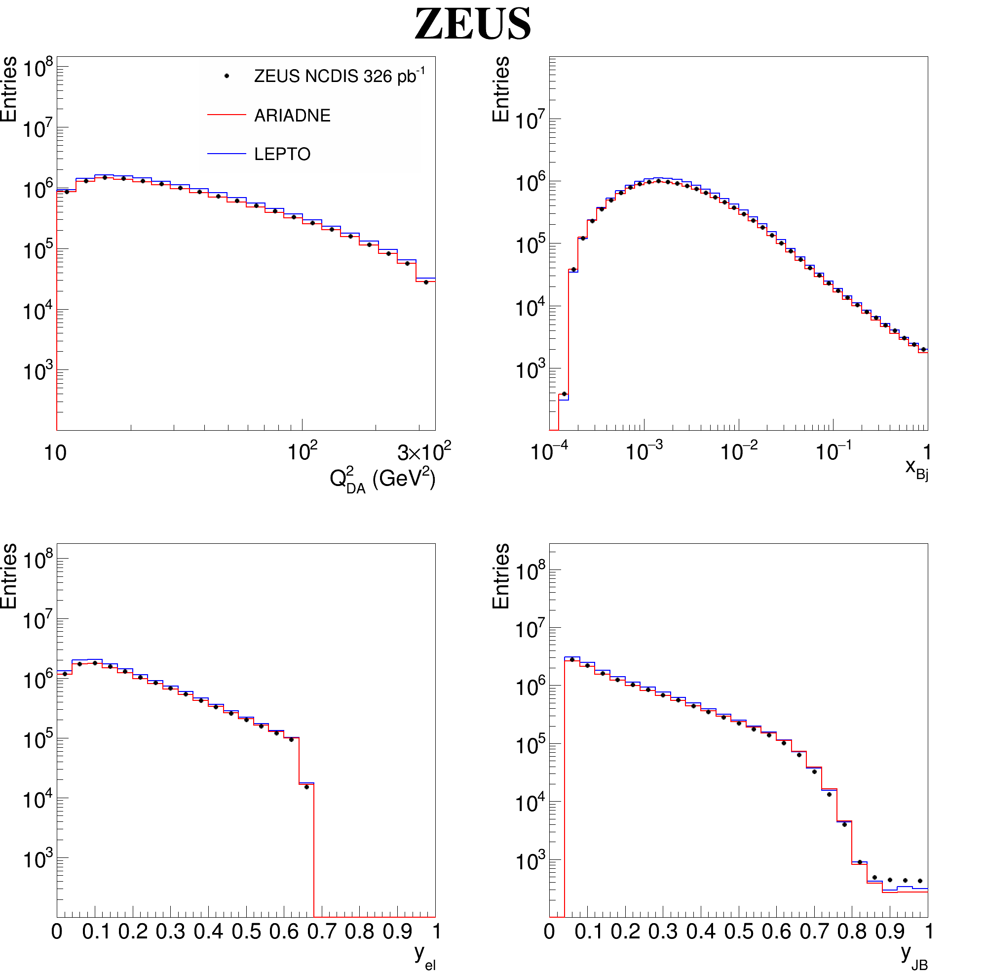
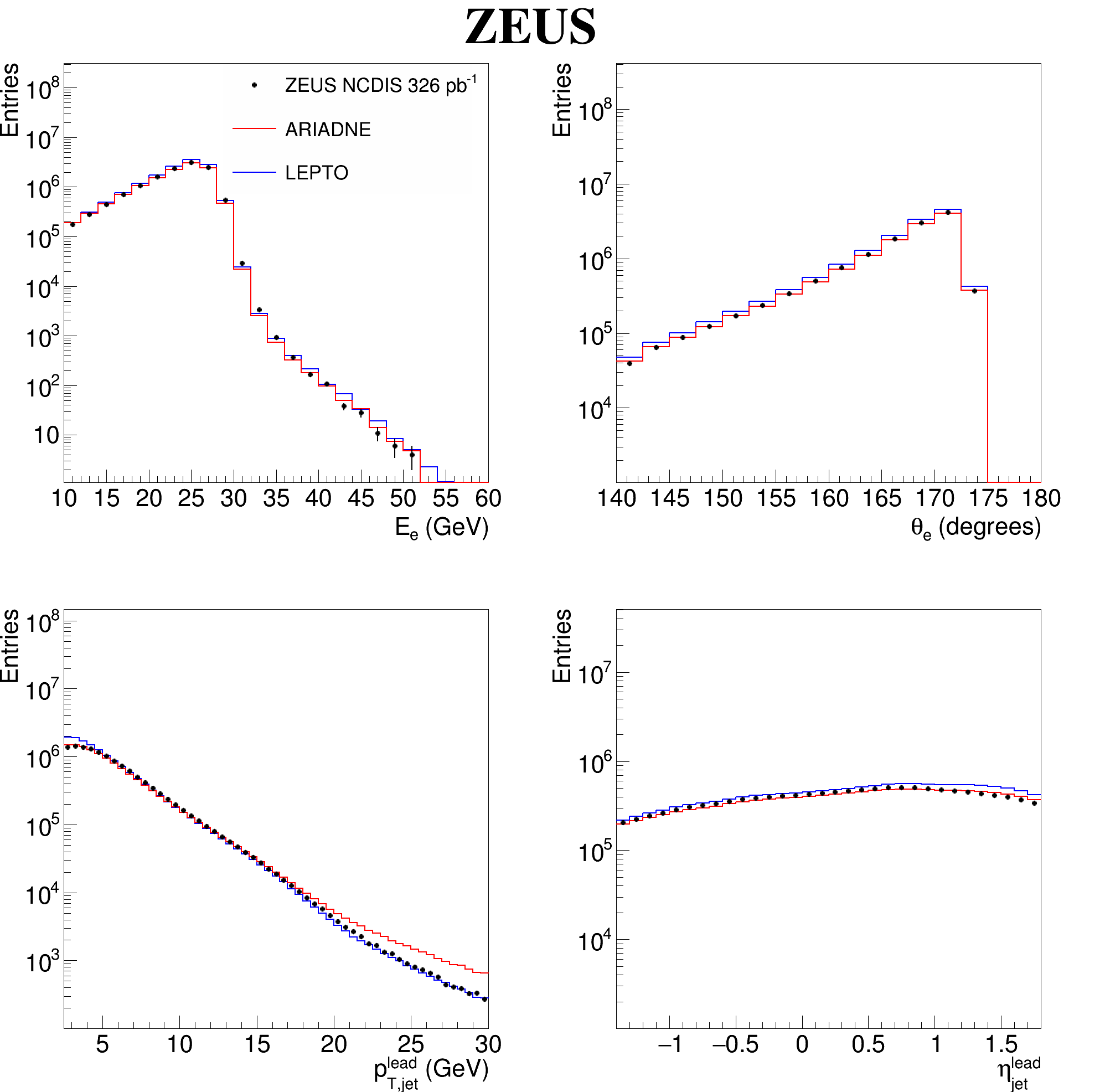
The final sample consisted of approximately DIS events with at least one jet that passed both the event-selection and jet-selection criteria. The contribution from remaining photoproduction events was found to be negligible after the DIS selection, being below . Comparisons of reconstructed DIS kinematic quantities between the data and MC simulations after all cuts are illustrated in Fig. 1 and for lepton and leading-jet quantities in Fig. 2. Both ARIADNE and LEPTO describe the data well. Differences between the two MC simulations were used to determine systematic uncertainties.
5 Signal extraction
Distributions of the azimuthal correlation angle obtained with the reconstructed electron and leading jet, , are shown in Fig. 3 for various jet-multiplicity ranges. The flattening of the event distribution as for multijet () events is consistent with the absence of the Born-level DIS process. The presence of additional jets, arising from processes, such as soft or hard gluon radiation, leads to deviations from a purely back-to-back configuration.
To extract the underlying hadron-level signal, a regularised unfolding was performed using the TUnfold package [58]. The migration matrix describes the detector and reconstruction effects on the hadron-level objects. The ARIADNE program was chosen to generate the input to the unfolding procedure because it provides a better description of the shapes of the distributions (see Fig. 3). Hadron jets were reconstructed in the laboratory frame using all the final-state ARIADNE particles666Final-state particles are defined as any stable particle whose lifetime is longer than . except for the scattered electron and neutrinos. The reconstruction was performed using the -clustering algorithm with the -recombination scheme in the longitudinally invariant inclusive mode [54], as implemented in the FastJet 3.4.0 package [55, 56]. The jet-radius parameter was set to . The kinematics of each event was obtained based on the scattered electron [50] and the correlation angle was calculated from the azimuthal angles of the true electron (after both initial- and final-state QED radiations) and the hadron jets. A detailed description of the unfolding scheme used in this analysis can be found in Appendix A.
Corrections were applied to account for three different effects arising from the migration of reconstructed quantities. First, events can falsely enter into the fiducial region of the measurement defined by the reconstructed kinematic quantities, resulting in an impurity in the signal. The impurity was estimated using the MC simulation and subtracted from the signal. Secondly, migrations can occur between and bins. A regularised unfolding, as implemented in TUnfold, was used to correct for this effect. Lastly, events that falsely fell out of the fiducial region defined by the hadron-level kinematics were corrected bin-wise by factors obtained from the simulation.
6 Systematic uncertainties
The following sources of systematic uncertainty were investigated:
-
•
the uncertainty associated with the choice of the regularisation parameter used in the unfolding procedure, as suggested by the TUnfold package, was propagated into the cross section. Its contribution to the total uncertainty was found to be less than throughout the entire range of , and was neglected;
-
•
the systematic effect of the uncertainty in the energy scale of the scattered electron measured in the calorimeter was estimated by varying the energy scale in the MC. Its effect was found to be negligible;
-
•
the jet-energy scale was varied within its uncertainty of for jet transverse energies < 10 GeV and for > 10 GeV [48] in the MC and found to be negligible;
-
•
the dependence on the specific values chosen for the event selection was estimated by varying the values by the reconstruction resolution;
-
•
the uncertainty related to the method used for estimating the impurity background was evaluated by performing the measurement using an alternative approach (see Appendix A). The systematic uncertainty associated with the choice of impurity estimation method was determined by comparing the results derived from the nominal and alternative methods;
-
•
the uncertainty associated with assumptions made in the ARIADNE simulation during the signal extraction process and in the cross-section calculation was evaluated by performing the measurement using an alternative MC sample based on the MEPS-LEPTO model. The difference in the resulting cross sections was taken as the systematic dependence on the simulation model.
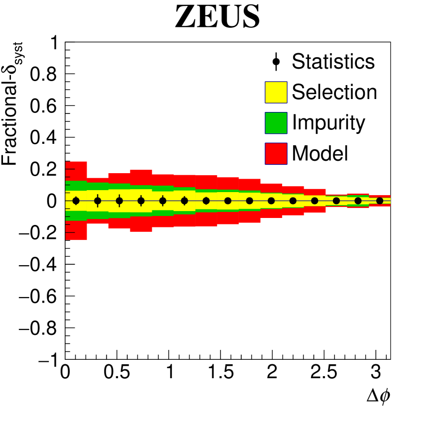
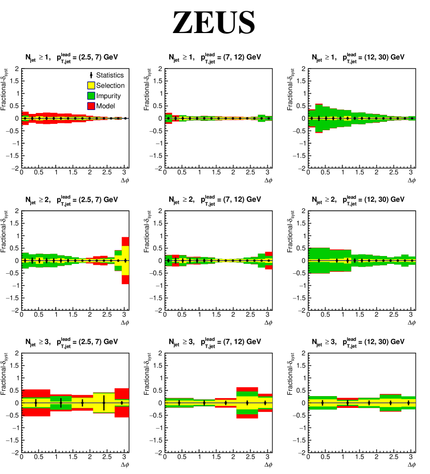
All significant uncertainties were symmetrised and added in quadrature to obtain the total systematic uncertainty. The individual systematic uncertainties compared to the statistical uncertainty are shown in Fig. 4 for the full fiducial region, while - and -dependent comparisons are provided in Appendix B.
7 Theory predictions
Fixed-order pQCD predictions for were computed by Borsa et al. [59] using the projection-to-Born (P2B) method [60, 61], as implemented in the POLDIS framework [17, 18]. The P2B method uses a dijet calculation at accuracy and a fully inclusive calculation at to produce an single-inclusive-jet () prediction. The results for dijet production, adapted for HERA parameters, were used to produce single-inclusive-jet calculations up to accuracy [17, 18]. These calculations were performed in the laboratory frame. The unpolarised PDF4LHC15 PDF set [62] was used as input to the calculation. Factorisation and renormalisation scales were chosen as . A central value of evaluated at was used. The theory uncertainty was determined from a seven-point scale variation with rescaling factors [, ].
These calculations were performed with massless parton jets. The predicted cross sections were corrected for the effects of hadronisation using results based on an ARIADNE MC study. A detailed description of the correction procedure is given in Appendix C.
8 Differential cross sections
The differential cross section of inclusive jet production in NC DIS, , was measured in the laboratory frame as a function of the azimuthal correlation angle between the scattered lepton and the leading jet, within the kinematic space defined by a range of the photon virtuality ; inelasticity ; electron energy ; electron polar angle ; jet transverse momentum ; and jet pseudorapidity as follows:
| (2) |
Here, represents the integrated luminosity, is the extracted signal as a distribution of corrected for migration effects, and is the width of each bin. The effects of both initial- and final-state QED radiation off the electron were estimated with RAPGAP (see Appendix D), and the corresponding QED correction factors, , were applied to extract the cross sections before such radiation. A non-leading jet may be falsely tagged as the leading jet if the true leading jet points too far forward or backward, e.g., through the beam pipe, or its transverse momentum exceeds the upper limit for reconstructed jets. The effects of incorrectly assigned leading jets were estimated with ARIADNE, and the corresponding correction factors, , were applied.
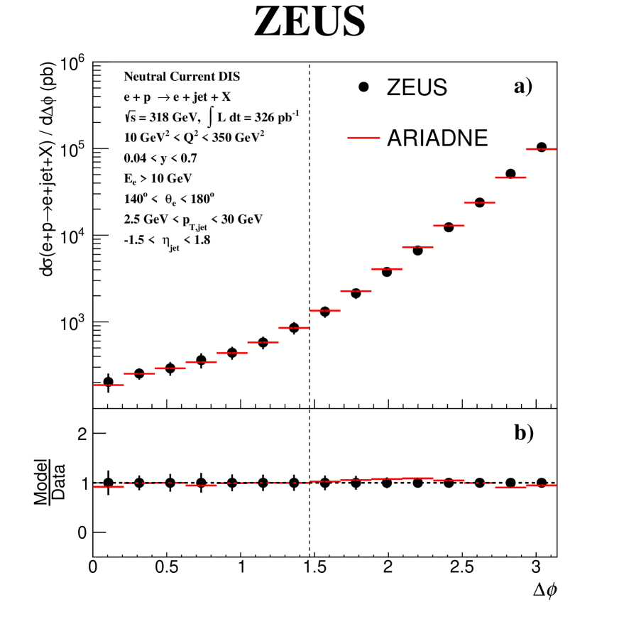
The inclusive () differential cross section, , of lepton–leading-jet pairs integrated over the studied fiducial region is presented as a function of the lepton–leading-jet correlation angle in Fig. 5. Perturbative calculations, treating up to or contributions (see Sec. 7), are compared to the measured cross sections within the range, . .
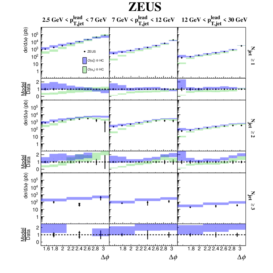
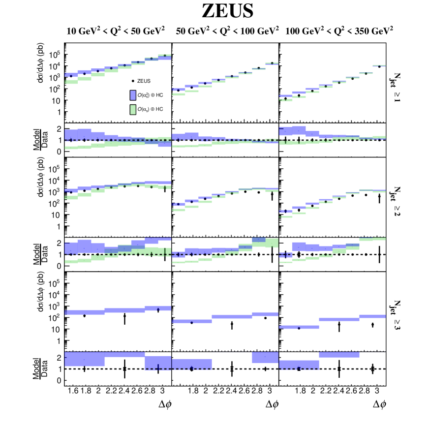
Additional measurements were performed for various ranges of , , and . The ranges were divided into three intervals: –, –, and –. The ranges were –, –, and –. The jet-multiplicity range was varied as , , and for each and range. Figures 6 and 7 present the differential cross sections for various ranges of and , and the respective theory predictions.
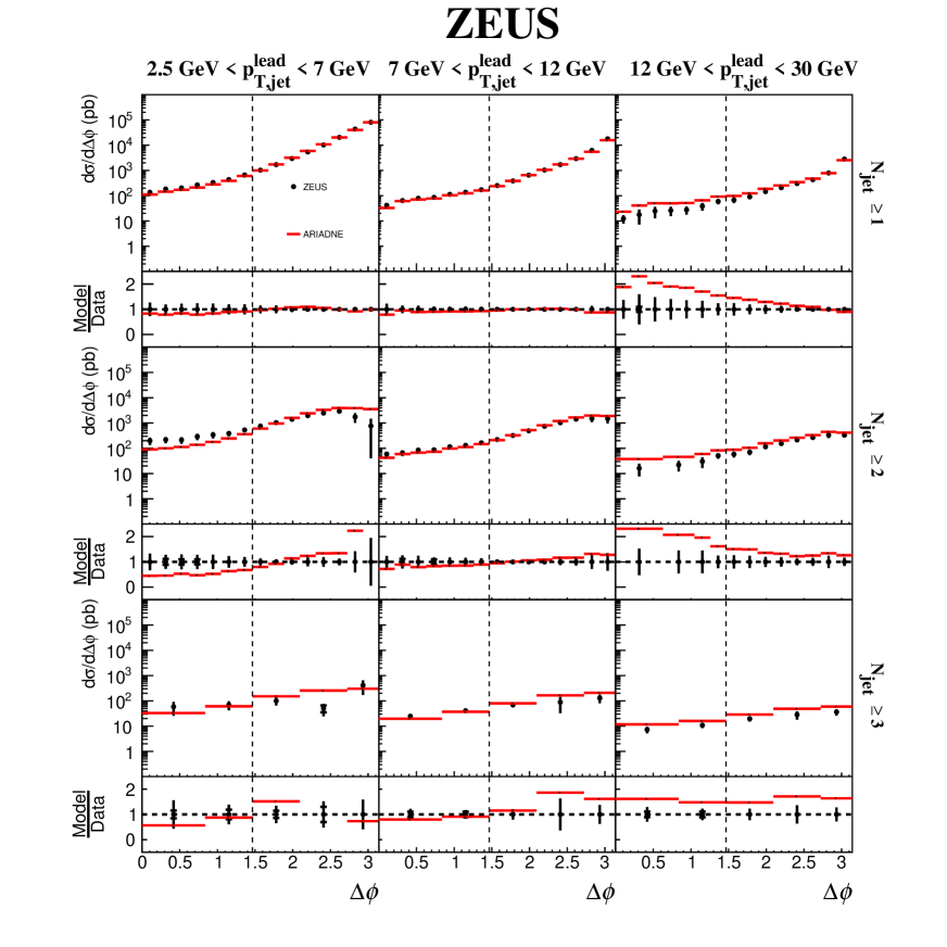
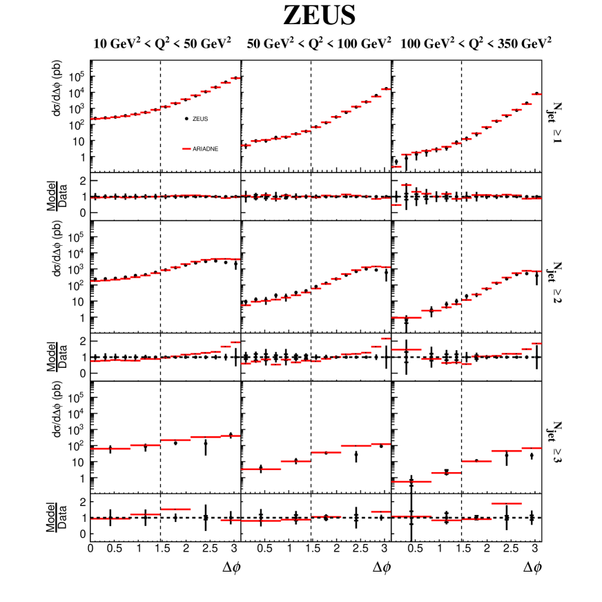
Figure 8 shows a comparison between the measured inclusive cross section and the prediction obtained from the ARIADNE LO+PS simulation. Comparisons between the data and ARIADNE cover the full range of from to . In Figs. 9 and 10, comparisons between the data and ARIADNE are presented for various ranges of and , respectively.
9 Discussion
Fixed-order calculations at and accuracy are compared to the inclusive measurement in Fig. 5. The corrections are NNLO for the last bin. An additional gluon is required for the leading jet to diverge from the back-to-back topology with respect to the scattered lepton, i.e., is LO and is NLO for . Here, the calculation demonstrates a clear improvement compared to , especially in the region where contributions from additional hard jet production significantly alter lepton–leading-jet production away from the back-to-back topology. On the other hand, no significant improvement is observed in the region , where substantial contributions from soft gluon radiation and intrinsic parton transverse momentum, , are expected. This is consistent with the findings of D [8], CMS [9, 10, 11], ATLAS [12], and H1 [14]. Figure 5 shows that perturbative predictions up to already provide a good description of the ZEUS data.
The fixed-order calculations were performed at the and accuracy for and , while only the calculation applies for , where this is effectively the leading order. The theory predictions are compared to the measurements in various ranges of and in Figs. 6 and 7, respectively. In all cases, the corrections significantly improved agreement with the data in the region , which is sensitive to additional hard jet production. This improvement extends into the low- regime, reaching down to . An enhancement of events displaying a reduced azimuthal correlation angle with increasing jet multiplicity is observed. This is expected and consistent with previous findings [11].
The slope of the measured cross section increases as a function of , as the higher-order contributions are suppressed for . For , the slope only increases with for . The scattered electron in DIS is analogous to one of the two jets in dijet production in hadron collisions if the electron is larger than the second-highest jet . Measurements from hadron colliders report a similar trend where the slope of the dijet cross section grows with increasing transverse momentum of the highest- jet [9, 10, 11, 12]. Furthermore, an improvement in agreement between the data and perturbative calculations is found for single-inclusive () events near with increasing . This finding is consistent with the expected suppression of soft gluon radiation and parton effects in the high- regime. No significant dependence of the shape of cross section on is observed in the present measurement.
In Fig. 8, the LO+PS prediction derived from the ARIADNE model is compared to the inclusive measurement. Here, there is a notable success of the LO+PS approach in describing higher-order processes characterised by and , even though they are not fully represented in the LO matrix elements. In Figs. 9 and 10, - and -dependent studies are illustrated. The performance of ARIADNE is comparable to that of perturbative calculations at accuracy across all ranges of , , and . These observations are consistent with previous findings [10, 11] and further support the validity of LO+PS approaches in describing a wide range of characteristics of the data. However, in contrast to the data, ARIADNE predicts an enhancement of events displaying a reduced azimuthal correlation angle with increasing . In particular, deviations emerge in for and low- for all ranges in . This observation might provide information on how parton showering could be improved to describe higher-order processes better, e.g., providing a basis for further tuning of hadronisation parameters.
10 Summary
Azimuthal correlations between the scattered lepton and the leading jet in NC DIS at HERA have been measured at ZEUS. The resulting distribution was unfolded to hadron level, correcting migration effects in the reconstructed kinematics. The differential cross section, , was derived from the unfolded distribution in the fiducial region defined by , , , , , and in the laboratory frame. The measurement was also performed for various ranges of , , and . The experimental uncertainty was dominated by the systematic dependence on the simulation model used in the unfolding procedure.
Perturbative calculations [59, 17, 18] up to and MC predictions based on the LO+PS approach implemented in the ARIADNE colour-dipole model have been compared to the data. The higher-order pQCD corrections show a significant improvement in describing regions that are driven by hard jet production. In addition, the excellent performance of perturbative calculations has been verified for jet transverse momentum down to . The LO+PS predictions by ARIADNE also describe the data well. The analysis procedures and results presented in this paper can be important in planning future experiments, e.g., at the Electron-Ion Collider (EIC) [63, 64].
Acknowledgements
We appreciate the contributions to the construction, maintenance and operation of the ZEUS detector of many people who are not listed as authors. The HERA machine group and the DESY computing staff are especially acknowledged for their success in providing excellent operation of the collider and the data-analysis environment. We thank the DESY directorate for their strong support and encouragement. {mcbibliography}10
References
- [1] H1 and ZEUS Collab., I. Abt et al., Eur. Phys. J. C 82, 243 (2022)
- [2] ZEUS Collab., I. Abt et al., Eur. Phys. J. C 83, 1082 (2023)
- [3] X. Liu et al., Phys. Rev. Lett. 122, 192003 (2019)
- [4] X. Liu et al., Phys. Rev. D 102, 094022 (2020)
- [5] ZEUS Collab., S. Chekanov et al., Phys. Lett. B 511, 19 (2001)
- [6] ZEUS Collab., S. Chekanov et al., Nucl. Phys. B 729, 492 (2005)
- [7] ZEUS Collab., S. Chekanov et al., Phys. Rev. D 76, 072011 (2007)
- [8] D Collab., V. Abazov et al., Phys. Rev. Lett. 94, 221801 (2005)
- [9] CMS Collab. V. Khachatryan et al., Phys. Rev. Lett. 106, 122003 (2011)
- [10] CMS Collab. V. Khachatryan et al., Eur. Phys. J. C 76, 536 (2016)
- [11] CMS Collab., A. Sirunyan et al., Eur. Phys. J. C 78, 566 (2018)
- [12] ATLAS Collab., G. Aad et al., Phys. Rev. Lett. 106, 172002 (2011)
- [13] ATLAS Collab. M. Aaboud et al., Phys. Rev. D 98, 092004 (2018)
- [14] H1 Collab. V. Andreev et al., Phys. Rev. Lett. 128, 132002 (2022)
- [15] STAR Collab., arXiv:2305.10359
- [16] H1 and ZEUS Collab., H. Abramowicz et al., JHEP 09, 149 (2015)
- [17] I. Borsa et al., Phys. Rev. Lett. 125, 082001 (2020)
- [18] I. Borsa et al., Phys. Rev. D 103, 014008 (2021)
- [19] L. Lönnblad, Comput. Phys. Commun. 71, 15 (1992)
- [20] ZEUS Collab., U. Holm (ed.), The ZEUS Detector. Status Report (unpublished), DESY (1993). http://www-zeus.desy.de/bluebook/bluebook.html
- [21] N. Harnew et al., Nucl. Instr. and Meth. A 279, 290 (1989)
- [22] B. Foster et al., Nucl. Phys. Proc. Suppl. B 32, 181 (1993)
- [23] B. Foster et al., Nucl. Instr. and Meth. A 338, 254 (1994)
- [24] A. Polini et al., Nucl. Instr. and Meth. A 581, 656 (2007)
- [25] S. Fourletov, Nucl. Instr. and Meth. A 535, 191 (2004)
- [26] M. Derrick et al., Nucl. Instr. and Meth. A 309, 77 (1991)
- [27] A. Andresen et al., Nucl. Instr. and Meth. A 309, 101 (1991)
- [28] A. Caldwell et al., Nucl. Instr. and Meth. A 321, 356 (1992)
- [29] A. Bernstein et al., Nucl. Instr. and Meth. A 336, 23 (1993)
- [30] J. Andruszków et al., Preprint DESY-92-066, DESY, 1992
- [31] ZEUS Collab., M. Derrick et al., Z. Phys. C 63, 391 (1994)
- [32] J. Andruszków et al., Acta Phys. Pol. B 32, 2025 (2001)
- [33] M. Helbich et al., Nucl. Instr. and Meth. A 565, 572 (2006)
- [34] H. Spiesberger. http://wwwthep.physik.uni-mainz.de/~hspiesb/djangoh/djangoh.html
- [35] CTEQ Collab., H. Lai et al., Eur. Phys. J. C 12, 375 (2000)
- [36] T. Sjöstrand, Comput. Phys. Commun. 82, 74 (1994)
- [37] ALEPH Collab., R. Barate et al., Phys. Rept. 294, 1 (1998)
- [38] A. Kwiatkowski et al., Comput. Phys. Commun. 69, 155 (1992)
- [39] G. Ingelman et al., Comput. Phys. Commun. 101, 108 (1997)
- [40] H. Jung, Comput. Phys. Commun. 86, 147 (1995)
- [41] T. Sjöstrand et al., JHEP 05, 026 (2006)
- [42] R. Brun et al., Technical Report CERN-DD/EE/84-1 (1987)
- [43] G. Hartner, Y. Iga. ZEUS Note 90-084
- [44] W.H. Smith et al., in the proceedings of Computing in High-Energy Physics (CHEP) (September 21-25, Annecy, France (1992)). DESY-92-150B
- [45] P. Allfrey et al., Nucl. Instrum. Meth. A 580, 1257 (2007)
- [46] ZEUS Collab., H. Abramowicz et al., Phys. Lett. B 691, 127 (2010)
- [47] ZEUS Collab., H. Abramowicz et al., Phys. Lett. B715, 88 (2012)
- [48] ZEUS Collab., H. Abramowicz et al., JHEP 01, 032 (2018)
- [49] U. Amaldi et al., ECFA Study of an ep Facility for Europe, pp. 377–414. (1979)
- [50] S. Bentvelsen et al., Workshop on Physics at HERA. (1992)
- [51] ZEUS Collab., M. Derrick et al., Phys. Lett. B 303, 183 (1993)
- [52] H. Abramowicz et al., Nucl. Instrum. Meth. A 365, 508 (1995)
- [53] S. Catani et al., Nucl. Phys. B 406, 187 (1993)
- [54] S. Ellis et al., Phys. Rev. D 48, 3160 (1993)
- [55] M. Cacciari et al., Eur. Phys. J. C 72, 1896 (2012)
- [56] M. Cacciari et al., Phys. Lett. B 641, 57 (2006)
- [57] ZEUS Collab., M. Wing, Frascati Phys. Ser. 21, 617 (2001)
- [58] S. Schmitt, JINST 7, T10003 (2012)
- [59] I. Borsa et al. Personal communications, 2021
- [60] M. Cacciari et al., Phys. Rev. Lett. 115, 082002 (2015)
- [61] M. Cacciari et al., Phys. Rev. Lett. 120, 139901 (2018)
- [62] J. Butterworth et al., J. Phys. G 43, 023001 (2016)
- [63] A. Accardi et al., Eur. Phys. J. A 52, 268 (2016)
- [64] R. Abdul Khalek et al., Nucl. Phys. A 1026, 122447 (2022)
| Inclusive | |||||||||||||
|---|---|---|---|---|---|---|---|---|---|---|---|---|---|
| ARIADNE | |||||||||||||
| 0.000 | 203 | 186 | |||||||||||
| 253 | 252 | ||||||||||||
| 291 | 291 | ||||||||||||
| 362 | 343 | ||||||||||||
| 440 | 438 | ||||||||||||
| 579 | 579 | ||||||||||||
| 854 | 853 | ||||||||||||
| 1313 | 1347 | 467 |
|
1677 |
|
||||||||
| 2139 | 2260 | 870 |
|
2863 |
|
||||||||
| 3770 | 4053 | 2060 |
|
4587 |
|
||||||||
| 6665 | 7262 | 4790 |
|
7608 |
|
||||||||
| 12347 | 12927 | 10300 |
|
13576 |
|
||||||||
| 23807 | 23742 | 22198 |
|
25778 |
|
||||||||
| 51160 | 46343 | 49672 |
|
48284 |
|
||||||||
| 103741 | 98392 | 111074 |
|
78854 |
|
||||||||
| ARIADNE | |||||||||||||
| 0.000 | 135 | 112 | |||||||||||
| 184 | 146 | ||||||||||||
| 204 | 172 | ||||||||||||
| 268 | 211 | ||||||||||||
| 334 | 280 | ||||||||||||
| 437 | 390 | ||||||||||||
| 665 | 608 | ||||||||||||
| 1030 | 1003 | 385 |
|
1231 |
|
||||||||
| 1707 | 1744 | 698 |
|
2250 |
|
||||||||
| 2980 | 3212 | 1653 |
|
3744 |
|
||||||||
| 5400 | 5936 | 4029 |
|
6333 |
|
||||||||
| 10246 | 10831 | 9071 |
|
11517 |
|
||||||||
| 20468 | 20304 | 20013 |
|
22078 |
|
||||||||
| 43489 | 40022 | 44709 |
|
40568 |
|
||||||||
| 80832 | 79998 | 91331 |
|
60442 |
|
||||||||
| 0.000 | 200 | 89.9 | |||||||||||
| 219 | 99.8 | ||||||||||||
| 213 | 113 | ||||||||||||
| 292 | 138 | ||||||||||||
| 341 | 179 | ||||||||||||
| 387 | 245 | ||||||||||||
| 533 | 362 | ||||||||||||
| 756 | 601 | 319 |
|
848 |
|
||||||||
| 1036 | 957 | 524 |
|
1476 |
|
||||||||
| 1407 | 1601 | 1147 |
|
2195 |
|
||||||||
| 1959 | 2422 | 2478 |
|
2990 |
|
||||||||
| 2487 | 3326 | 4011 |
|
4241 |
|
||||||||
| 2922 | 3923 | 4420 |
|
5553 |
|
||||||||
| 1746 | 3900 | 3165 |
|
5640 |
|
||||||||
| 766 | 3549 | 2140 |
|
5052 |
|
||||||||
| 0.000 | 58.3 | 33.0 | |||||||||||
| 69.3 | 60.7 | ||||||||||||
| 99.7 | 151 | 178 |
|
||||||||||
| 50.5 | 256 | 297 |
|
||||||||||
| 412 | 302 | 474 |
|
||||||||||
| ARIADNE | |||||||||||||
| 0.000 | 41.8 | 33.0 | |||||||||||
| 64.5 | 61.5 | ||||||||||||
| 79.4 | 70.8 | ||||||||||||
| 86.3 | 77.9 | ||||||||||||
| 114 | 104 | ||||||||||||
| 138 | 126 | ||||||||||||
| 173 | 161 | ||||||||||||
| 253 | 240 | 39.0 |
|
286 |
|
||||||||
| 387 | 387 | 125 |
|
417 |
|
||||||||
| 654 | 654 | 349 |
|
619 |
|
||||||||
| 1040 | 1063 | 650 |
|
1049 |
|
||||||||
| 1707 | 1745 | 1102 |
|
1771 |
|
||||||||
| 2945 | 2918 | 2033 |
|
3149 |
|
||||||||
| 6252 | 5481 | 4663 |
|
6201 |
|
||||||||
| 17979 | 15793 | 17133 |
|
16157 |
|
||||||||
| 0.000 | 58.9 | 42.4 | |||||||||||
| 65.9 | 58.9 | ||||||||||||
| 84.8 | 67.2 | ||||||||||||
| 87.4 | 72.7 | ||||||||||||
| 115 | 97.5 | ||||||||||||
| 131 | 112 | ||||||||||||
| 164 | 147 | ||||||||||||
| 222 | 210 | 39.8 |
|
261 |
|
||||||||
| 322 | 325 | 110 |
|
386 |
|
||||||||
| 494 | 524 | 291 |
|
542 |
|
||||||||
| 744 | 808 | 541 |
|
854 |
|
||||||||
| 1025 | 1195 | 918 |
|
1345 |
|
||||||||
| 1423 | 1664 | 1629 |
|
2123 |
|
||||||||
| 1498 | 1973 | 2358 |
|
2825 |
|
||||||||
| 1487 | 1904 | 1900 |
|
2822 |
|
||||||||
| 0.000 | 24.6 | 19.6 | |||||||||||
| 40.7 | 37.0 | ||||||||||||
| 69.2 | 79.9 | 92.4 |
|
||||||||||
| 88.4 | 165 | 196 |
|
||||||||||
| 129 | 208 | 287 |
|
||||||||||
| ARIADNE | |||||||||||||
| 0.000 | 12.5 | 23.5 | |||||||||||
| 17.8 | 41.2 | ||||||||||||
| 24.8 | 50.6 | ||||||||||||
| 26.3 | 50.1 | ||||||||||||
| 27.8 | 51.6 | ||||||||||||
| 38.7 | 65.9 | ||||||||||||
| 59.7 | 92.5 | ||||||||||||
| 68.0 | 98.8 | 11.4 |
|
101 |
|
||||||||
| 90.7 | 125 | 54.1 |
|
90.0 |
|
||||||||
| 146 | 189 | 104 |
|
144 |
|
||||||||
| 209 | 256 | 150 |
|
223 |
|
||||||||
| 304 | 346 | 211 |
|
324 |
|
||||||||
| 434 | 476 | 326 |
|
500 |
|
||||||||
| 796 | 782 | 635 |
|
889 |
|
||||||||
| 2832 | 2550 | 3103 |
|
3183 |
|
||||||||
| 0.000 | 16.2 | 37.5 | |||||||||||
| 22.1 | 45.8 | ||||||||||||
| 30.4 | 59.5 | ||||||||||||
| 51.1 | 82.6 | ||||||||||||
| 58.1 | 87.6 | 9.65 |
|
92.1 |
|
||||||||
| 70.5 | 105 | 42.6 |
|
86.0 |
|
||||||||
| 115 | 157 | 81.2 |
|
126 |
|
||||||||
| 154 | 204 | 116 |
|
187 |
|
||||||||
| 214 | 262 | 160 |
|
256 |
|
||||||||
| 266 | 333 | 242 |
|
369 |
|
||||||||
| 333 | 446 | 413 |
|
558 |
|
||||||||
| 330 | 416 | 487 |
|
649 |
|
||||||||
| 0.000 | 7.26 | 11.7 | |||||||||||
| 10.8 | 16.0 | ||||||||||||
| 19.4 | 28.6 | 28.1 |
|
||||||||||
| 28.3 | 48.5 | 55.7 |
|
||||||||||
| 36.2 | 59.4 | 84.9 |
|
||||||||||
| ARIADNE | |||||||||||||
| 0.000 | 239 | 224 | |||||||||||
| 256 | 245 | ||||||||||||
| 287 | 281 | ||||||||||||
| 349 | 329 | ||||||||||||
| 435 | 421 | ||||||||||||
| 560 | 553 | ||||||||||||
| 817 | 814 | ||||||||||||
| 1247 | 1273 | 426 |
|
1564 |
|
||||||||
| 2010 | 2105 | 791 |
|
2641 |
|
||||||||
| 3448 | 3698 | 1849 |
|
4157 |
|
||||||||
| 5982 | 6465 | 4221 |
|
6746 |
|
||||||||
| 10842 | 11275 | 8932 |
|
11815 |
|
||||||||
| 20629 | 20400 | 18943 |
|
21961 |
|
||||||||
| 42923 | 39260 | 41570 |
|
39374 |
|
||||||||
| 77642 | 75775 | 83056 |
|
56349 |
|
||||||||
| 0.000 | 233 | 176 | |||||||||||
| 242 | 190 | ||||||||||||
| 260 | 215 | ||||||||||||
| 309 | 245 | ||||||||||||
| 391 | 306 | ||||||||||||
| 436 | 390 | ||||||||||||
| 611 | 543 | ||||||||||||
| 867 | 837 | 328 |
|
1158 |
|
||||||||
| 1199 | 1259 | 572 |
|
1835 |
|
||||||||
| 1722 | 1993 | 1311 |
|
2523 |
|
||||||||
| 2343 | 2825 | 2726 |
|
3243 |
|
||||||||
| 2898 | 3672 | 4161 |
|
4455 |
|
||||||||
| 3121 | 4150 | 4348 |
|
5799 |
|
||||||||
| 2536 | 4207 | 3215 |
|
6152 |
|
||||||||
| 2068 | 3984 | 2519 |
|
5783 |
|
||||||||
| 0.000 | 67.2 | 63.1 | |||||||||||
| 86.1 | 103 | ||||||||||||
| 142 | 217 | 257 |
|
||||||||||
| 132 | 334 | 391 |
|
||||||||||
| 467 | 393 | 593 |
|
||||||||||
| ARIADNE | |||||||||||||
| 0.000 | 4.73 | 4.97 | |||||||||||
| 9.53 | 9.33 | ||||||||||||
| 9.84 | 10.8 | ||||||||||||
| 15.2 | 13.1 | ||||||||||||
| 16.0 | 17.1 | ||||||||||||
| 26.0 | 25.2 | ||||||||||||
| 37.1 | 37.7 | ||||||||||||
| 70.8 | 67.9 | 32.0 |
|
84.1 |
|
||||||||
| 127 | 136 | 59.8 |
|
162 |
|
||||||||
| 290 | 297 | 156 |
|
313 |
|
||||||||
| 563 | 636 | 411 |
|
623 |
|
||||||||
| 1209 | 1284 | 980 |
|
1246 |
|
||||||||
| 2526 | 2553 | 2261 |
|
2572 |
|
||||||||
| 6302 | 5419 | 5465 |
|
5615 |
|
||||||||
| 16928 | 15663 | 16726 |
|
13954 |
|
||||||||
| 0.000 | 9.07 | 5.45 | |||||||||||
| 12.5 | 9.14 | ||||||||||||
| 11.9 | 10.2 | ||||||||||||
| 22.7 | 12.2 | ||||||||||||
| 19.0 | 16.2 | ||||||||||||
| 34.0 | 23.0 | ||||||||||||
| 43.6 | 34.1 | ||||||||||||
| 80.6 | 60.3 | 24.3 |
|
74.7 |
|
||||||||
| 129 | 117 | 47.2 |
|
151 |
|
||||||||
| 237 | 239 | 128 |
|
290 |
|
||||||||
| 407 | 479 | 345 |
|
556 |
|
||||||||
| 692 | 834 | 805 |
|
998 |
|
||||||||
| 989 | 1267 | 1582 |
|
1644 |
|
||||||||
| 855 | 1413 | 1776 |
|
2005 |
|
||||||||
| 593 | 1279 | 1176 |
|
1817 |
|
||||||||
| 0.000 | 4.14 | 3.33 | |||||||||||
| 11.7 | 10.3 | ||||||||||||
| 34.8 | 36.5 | 44.2 |
|
||||||||||
| 27.1 | 95.5 | 113 |
|
||||||||||
| 89.1 | 122 | 185 |
|
||||||||||
| ARIADNE | |||||||||||||
| 0.000 | 0.486 | 0.232 | |||||||||||
| 0.771 | 1.33 | ||||||||||||
| 1.37 | 1.79 | ||||||||||||
| 1.92 | 2.28 | ||||||||||||
| 2.78 | 2.79 | ||||||||||||
| 3.46 | 4.07 | ||||||||||||
| 7.75 | 6.68 | ||||||||||||
| 13.4 | 12.4 | 10.3 |
|
23.6 |
|
||||||||
| 25.4 | 27.9 | 19.0 |
|
45.8 |
|
||||||||
| 62.3 | 68.5 | 50.5 |
|
95.1 |
|
||||||||
| 158 | 168 | 142 |
|
208 |
|
||||||||
| 337 | 377 | 365 |
|
455 |
|
||||||||
| 758 | 820 | 898 |
|
1029 |
|
||||||||
| 2120 | 1850 | 2307 |
|
2472 |
|
||||||||
| 8500 | 7567 | 10525 |
|
9396 |
|
||||||||
| 0.000 | 0.621 | 0.912 | |||||||||||
| 2.84 | 2.54 | ||||||||||||
| 6.29 | 4.05 | ||||||||||||
| 9.61 | 6.41 | ||||||||||||
| 20.5 | 11.7 | 6.18 |
|
18.9 |
|
||||||||
| 24.6 | 25.6 | 12.6 |
|
40.0 |
|
||||||||
| 57.2 | 60.1 | 37.1 |
|
88.0 |
|
||||||||
| 129 | 139 | 114 |
|
193 |
|
||||||||
| 239 | 290 | 303 |
|
405 |
|
||||||||
| 449 | 542 | 742 |
|
829 |
|
||||||||
| 510 | 763 | 1294 |
|
1342 |
|
||||||||
| 382 | 706 | 991 |
|
1312 |
|
||||||||
| 0.000 | 0.518 | 0.553 | |||||||||||
| 2.34 | 1.96 | ||||||||||||
| 11.4 | 10.4 | 14.0 |
|
||||||||||
| 24.3 | 45.6 | 64.9 |
|
||||||||||
| 24.3 | 68.2 | 122 |
|
||||||||||


Appendix A Unfolding
The event kinematics obtained from the detector response is subject to effects arising from imperfect resolution and inefficiency of the chosen reconstruction scheme. A three-level unfolding scheme was employed in order to map the yield of reconstructed lepton–leading-jet pairs to that of true electrons and hadron jets that are free of these effects.
Each DIS event can be categorised into one of four groups:
-
•
— the event enters into both the fiducial region defined by the kinematics reconstructed with the detector response and the region defined by the true electron and final-state hadrons;
-
•
— it falsely falls outside the fiducial region defined by the detector-level kinematics;
-
•
— it falsely falls into the detector-level fiducial region;
-
•
— it correctly falls outside the detector-level fiducial region.
The distribution of , also referred to as impurity background, was first subtracted from the measured signal () to extract . The impurity background was estimated using two different methods: a) the relative fraction of the impurity background in the MC simulation was taken as the background in data, . The resulting distribution was considered the nominal impurity background, b) the absolute yield derived from the simulation was directly taken as the background in data, . The difference in the background extracted with these methods was taken as the systematic uncertainty in the impurity estimate.
This was followed by a two-dimensional regularised unfolding technique implemented in the TUnfold package [58] to account for migration of and within the extracted events. With defined as a distribution of a chosen quantity reconstructed from the detector response, as the distribution of the same quantity defined at the hadron level, and as the response matrix, a folding equation can be formed as . A regularised unfolding is performed by minimising the following expression:
| (3) |
where represents the covariance matrix of the quantity , the parameter is referred to as the regularisation parameter, is the normalised truth-level distribution obtained from , and the matrix contains the regularisation conditions.
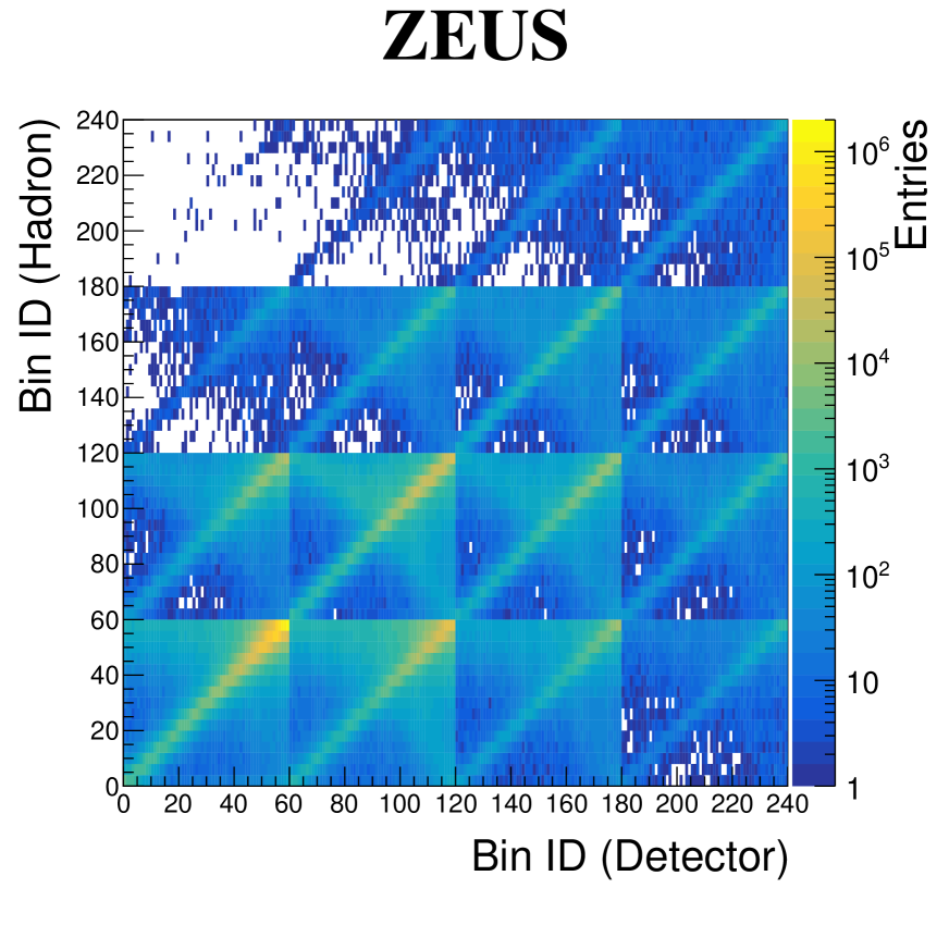
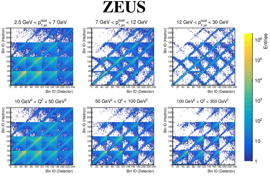
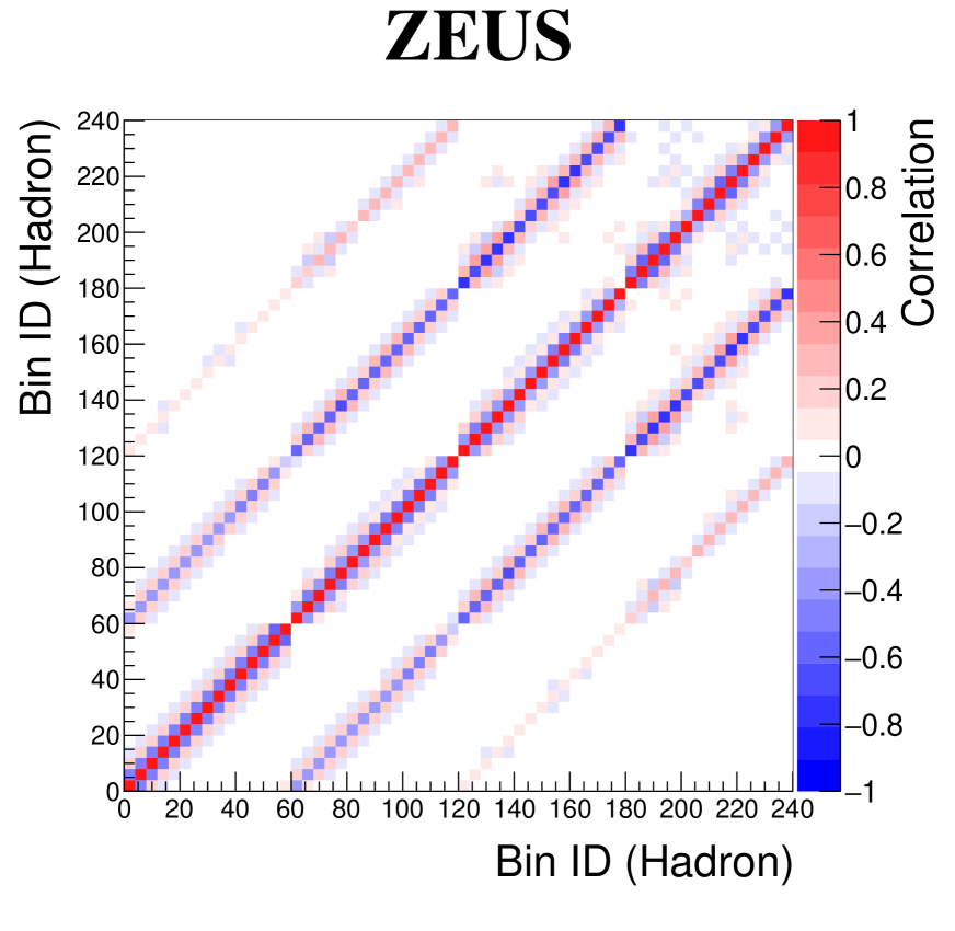
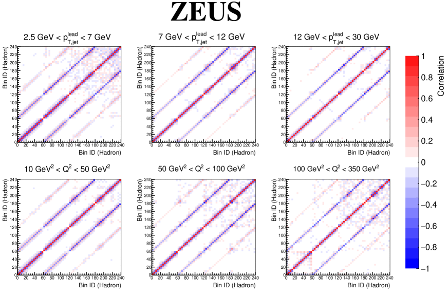
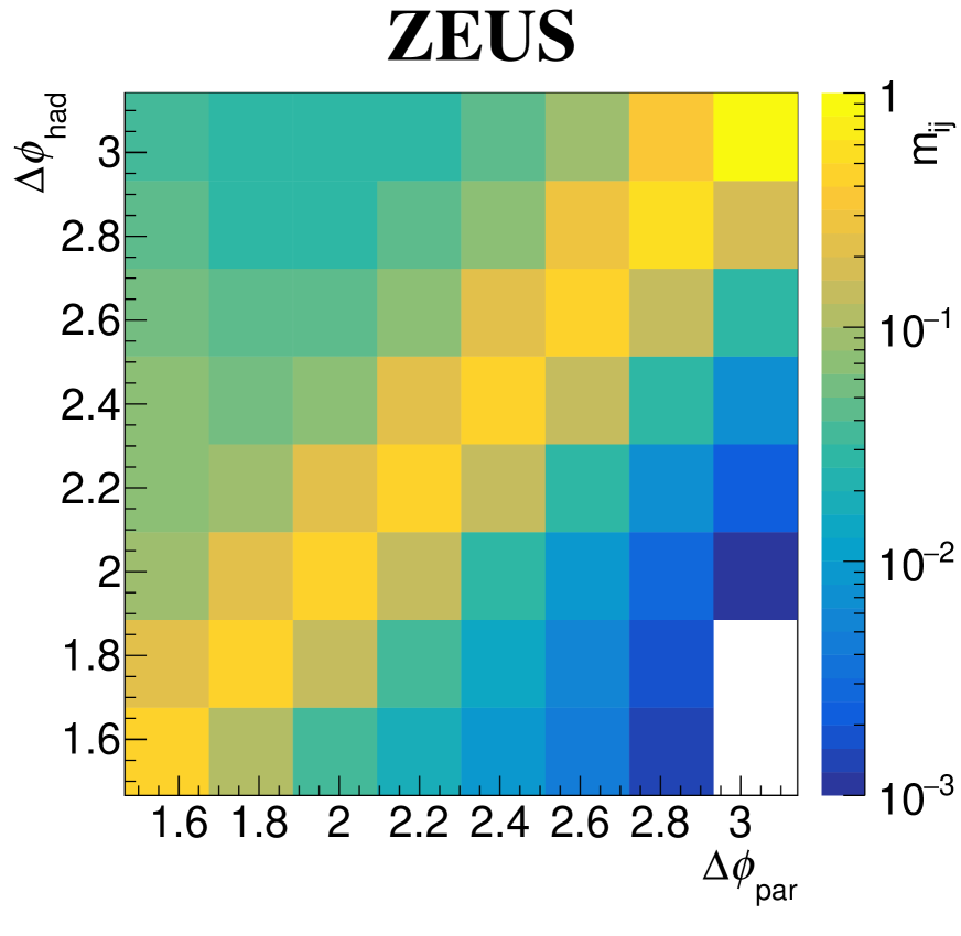
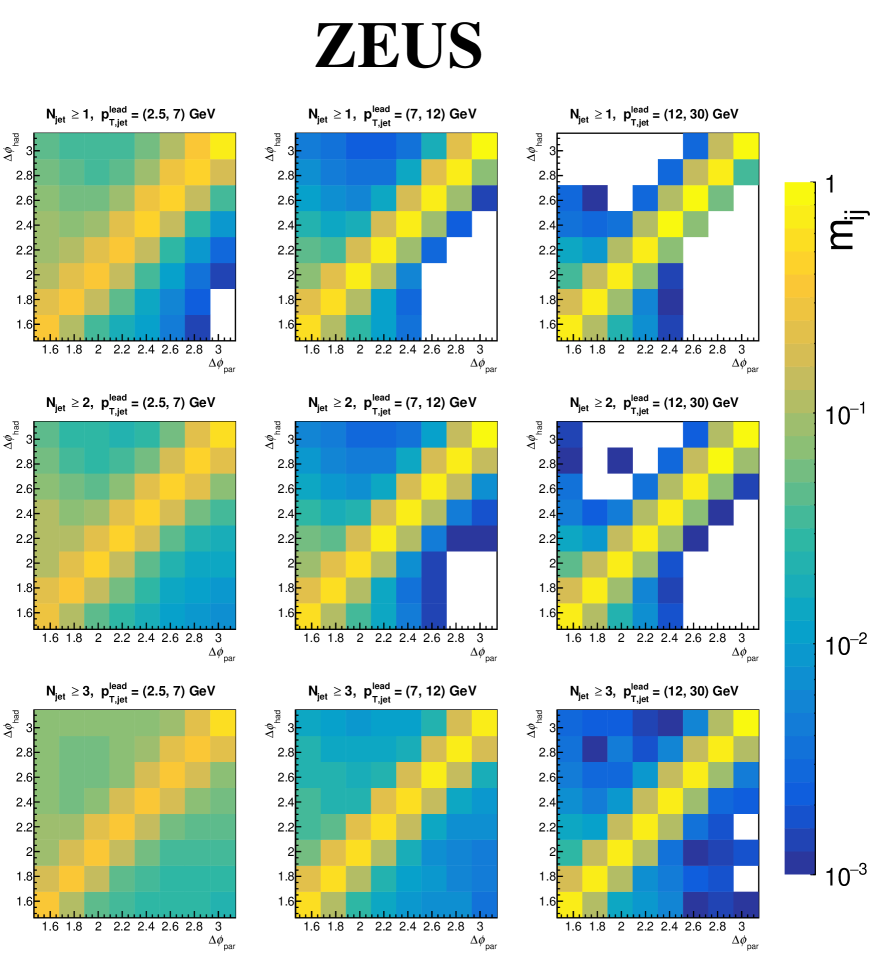
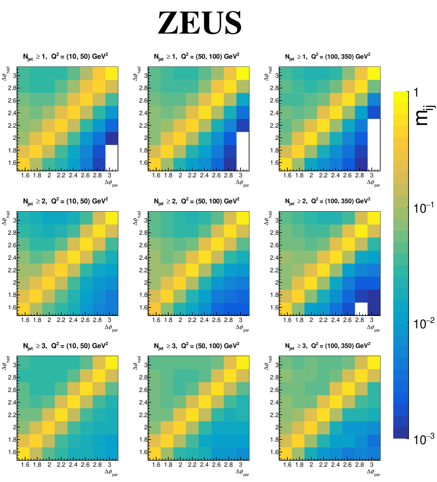
The first term in equation 3 represents the least-square minimisation of the folding equation. In this measurement, the response matrix was constructed from the migration matrix, . The two-dimensional information of and from each event in the MC simulation was mapped onto a one-dimensional axis. The values in were determined by mapping the hadron-level distribution of to the detector-level distribution. Figures 11 and 12 represent the migration matrices for the inclusive and /-dependent measurements, respectively. Matrices of statistical correlation coefficients of the unfolded lepton–leading-jet yield for the inclusive and /-dependent measurements are shown in Figs. 13 and 14, respectively. Typically, negative correlations of are observed in the adjacent and bins due to detector and reconstruction effects.
The least-square approach is prone to large fluctuations in the resulting distribution. The regularisation term, shown as the second term in equation 3, dampens this fluctuation based on the regularisation parameter and the regularisation conditions. In this measurement, the regularisation was performed on the second derivatives; the diagonal elements of , , were set to , , and . The regularisation parameter, , was obtained using the -curve scan method, i.e., the value of is chosen from the point where the curvature is maximal in the graph of from a simplified form of equation 3, . The term typically contributes to to the value of .
Finally, the efficiency of the ZEUS detector and reconstruction procedure was estimated with the MC simulation as . The unfolding procedure described above can be expressed as follows:
| (4) |
where represents the regularised unfolding, is the distribution of as reconstructed from the detector response, is the estimated impurity background, and is the hadron-level distribution of that is free of detector and reconstruction effects.
Appendix B Systematic uncertainties
Comparisons of the estimated systematic uncertanties to the statistical uncertainty are shown in Figs. 15 and 16 for the - and -dependent measurements, respectively.

Appendix C Hadronisation correction
Corrections were applied to the parton-level calculations to account for hadronisation effects. Parton-level jets were found from the collision information provided by the ARIADNE simulation with the -clustering algorithm with in the massless mode. This jet definition is the same as used in the perturbative calculations. A two-dimensional distribution of hadron-level correlation angle, , versus parton-level angle, , was formed for each , , and range. This distribution was normalised along the axis, ensuring that the sum of each column, , was equal to unity. Thus, each element in the matrix represents the probability of a parton-level pair in bin contributing to the hadron-level yield in bin . These distributions are shown in Figs. 17, 18, and 19. In order to correct for the migration of the kinematic quantities that define the fiducial region of the measurement, two additional correction factors, denoted as and , were computed using the MC simulation. The factor is the fraction of parton-level lepton–leading-jet pairs with a matching hadron-level pair over the total parton-level yield. On the other hand, is the fraction of hadron-level pairs with a matching parton-level pair over the total hadron-level yield. Hadron-level predictions were obtained from the perturbative calculations at parton level by using the following expression:
| (5) |
In this expression, represents the hadron-level differential cross section in bin to be directly compared to the measurement, and represents the parton-level differential cross section in bin obtained with the P2B method.
The dependence on model-specific assumptions made in the ARIADNE simulation was tested by repeating the hadronisation correction with the LEPTO simulation. The difference in the result derived using the two models was found to be at maximum. This was taken as an additional source of uncertainty in the predictions and added in quadrature to the uncertainty arising from scale variations.
Appendix D QED radiation correction
The resulting cross sections were corrected to QED Born-level, which is defined by the absence of QED-radiative effects, while including the scale dependence of the electromagnetic coupling. Corresponding MC samples were generated using the RAPGAP 3.308 event generator [40] with QED radiation simulated by HERACLES [38]. Bin-wise correction factors were determined by comparing the cross sections derived from these samples to those from the nominal MC samples. The resulting correction factors, , are listed in Table 8 for the inclusive cross section, Table 9 for the -dependent cross sections, and Table 10 for the -dependent cross sections.
| Inclusive | |||
|---|---|---|---|
| 0.000 | 0.209 | 0.766 | |
| 0.209 | 0.419 | 0.949 | |
| 0.419 | 0.628 | 0.979 | |
| 0.628 | 0.838 | 0.987 | |
| 0.838 | 1.047 | 1.010 | |
| 1.047 | 1.257 | 0.992 | |
| 1.257 | 1.466 | 1.007 | |
| 1.466 | 1.676 | 1.003 | |
| 1.676 | 1.885 | 1.004 | |
| 1.885 | 2.094 | 1.016 | |
| 2.094 | 2.304 | 1.019 | |
| 2.304 | 2.513 | 1.012 | |
| 2.513 | 2.723 | 1.014 | |
| 2.723 | 2.932 | 1.018 | |
| 2.932 | 3.142 | 1.009 | |
| 0.000 | 0.209 | 0.814 | 0.000 | 0.209 | 0.548 | 0.000 | 0.209 | 0.483 | |
| 0.209 | 0.419 | 0.953 | 0.209 | 0.419 | 0.927 | 0.209 | 0.419 | 0.856 | |
| 0.419 | 0.628 | 0.979 | 0.419 | 0.628 | 0.980 | 0.419 | 0.628 | 0.989 | |
| 0.628 | 0.838 | 0.990 | 0.628 | 0.838 | 0.982 | 0.628 | 0.838 | 0.897 | |
| 0.838 | 1.047 | 1.008 | 0.838 | 1.047 | 1.061 | 0.838 | 1.047 | 0.884 | |
| 1.047 | 1.257 | 0.990 | 1.047 | 1.257 | 1.019 | 1.047 | 1.257 | 0.977 | |
| 1.257 | 1.466 | 1.006 | 1.257 | 1.466 | 0.981 | 1.257 | 1.466 | 1.154 | |
| 1.466 | 1.676 | 1.007 | 1.466 | 1.676 | 0.975 | 1.466 | 1.676 | 0.979 | |
| 1.676 | 1.885 | 1.004 | 1.676 | 1.885 | 1.012 | 1.676 | 1.885 | 0.936 | |
| 1.885 | 2.094 | 1.016 | 1.885 | 2.094 | 1.024 | 1.885 | 2.094 | 1.005 | |
| 2.094 | 2.304 | 1.019 | 2.094 | 2.304 | 1.016 | 2.094 | 2.304 | 0.984 | |
| 2.304 | 2.513 | 1.012 | 2.304 | 2.513 | 1.012 | 2.304 | 2.513 | 0.982 | |
| 2.513 | 2.723 | 1.018 | 2.513 | 2.723 | 0.989 | 2.513 | 2.723 | 0.907 | |
| 2.723 | 2.932 | 1.026 | 2.723 | 2.932 | 0.970 | 2.723 | 2.932 | 0.877 | |
| 2.932 | 3.142 | 1.030 | 2.932 | 3.142 | 0.942 | 2.932 | 3.142 | 0.828 | |
| 0.000 | 0.209 | 0.926 | 0.000 | 0.209 | 0.728 | 0.000 | 0.628 | 0.855 | |
| 0.209 | 0.419 | 0.966 | 0.209 | 0.419 | 0.955 | ||||
| 0.419 | 0.628 | 0.971 | 0.419 | 0.628 | 0.998 | ||||
| 0.628 | 0.838 | 0.974 | 0.628 | 0.838 | 0.995 | 0.628 | 1.047 | 0.908 | |
| 0.838 | 1.047 | 0.997 | 0.838 | 1.047 | 1.078 | ||||
| 1.047 | 1.257 | 0.978 | 1.047 | 1.257 | 1.005 | 1.047 | 1.257 | 0.987 | |
| 1.257 | 1.466 | 0.983 | 1.257 | 1.466 | 1.003 | 1.257 | 1.466 | 1.171 | |
| 1.466 | 1.676 | 1.032 | 1.466 | 1.676 | 0.981 | 1.466 | 1.676 | 0.992 | |
| 1.676 | 1.885 | 1.022 | 1.676 | 1.885 | 1.006 | 1.676 | 1.885 | 0.924 | |
| 1.885 | 2.094 | 1.044 | 1.885 | 2.094 | 1.023 | 1.885 | 2.094 | 1.019 | |
| 2.094 | 2.304 | 1.027 | 2.094 | 2.304 | 1.026 | 2.094 | 2.304 | 0.987 | |
| 2.304 | 2.513 | 1.014 | 2.304 | 2.513 | 1.009 | 2.304 | 2.513 | 0.991 | |
| 2.513 | 2.723 | 0.999 | 2.513 | 2.723 | 0.982 | 2.513 | 2.723 | 0.910 | |
| 2.723 | 2.932 | 1.011 | 2.723 | 2.932 | 0.961 | 2.723 | 2.932 | 0.869 | |
| 2.932 | 3.142 | 1.003 | 2.932 | 3.142 | 0.930 | 2.932 | 3.142 | 0.654 | |
| 0.000 | 0.838 | 0.969 | 0.000 | 0.838 | 0.847 | 0.000 | 0.838 | 0.884 | |
| 0.838 | 1.466 | 0.984 | 0.838 | 1.466 | 0.998 | 0.838 | 1.466 | 0.939 | |
| 1.466 | 2.094 | 1.064 | 1.466 | 2.094 | 1.009 | 1.466 | 2.094 | 0.994 | |
| 2.094 | 2.723 | 1.017 | 2.094 | 2.723 | 0.966 | 2.094 | 2.723 | 0.934 | |
| 2.723 | 3.142 | 0.983 | 2.723 | 3.142 | 0.928 | 2.723 | 3.142 | 0.764 | |
| 0.000 | 0.209 | 0.930 | 0.000 | 0.209 | 0.486 | 0.000 | 0.209 | 0.118 | |
| 0.209 | 0.419 | 0.969 | 0.209 | 0.419 | 0.886 | 0.209 | 0.419 | 0.577 | |
| 0.419 | 0.628 | 0.994 | 0.419 | 0.628 | 0.941 | 0.419 | 0.628 | 0.655 | |
| 0.628 | 0.838 | 0.998 | 0.628 | 0.838 | 0.966 | 0.628 | 0.838 | 0.710 | |
| 0.838 | 1.047 | 1.023 | 0.838 | 1.047 | 0.971 | 0.838 | 1.047 | 0.715 | |
| 1.047 | 1.257 | 1.003 | 1.047 | 1.257 | 0.964 | 1.047 | 1.257 | 0.727 | |
| 1.257 | 1.466 | 1.019 | 1.257 | 1.466 | 0.959 | 1.257 | 1.466 | 0.742 | |
| 1.466 | 1.676 | 1.013 | 1.466 | 1.676 | 0.990 | 1.466 | 1.676 | 0.740 | |
| 1.676 | 1.885 | 1.014 | 1.676 | 1.885 | 0.987 | 1.676 | 1.885 | 0.747 | |
| 1.885 | 2.094 | 1.028 | 1.885 | 2.094 | 0.994 | 1.885 | 2.094 | 0.748 | |
| 2.094 | 2.304 | 1.031 | 2.094 | 2.304 | 1.000 | 2.094 | 2.304 | 0.757 | |
| 2.304 | 2.513 | 1.025 | 2.304 | 2.513 | 1.007 | 2.304 | 2.513 | 0.760 | |
| 2.513 | 2.723 | 1.028 | 2.513 | 2.723 | 1.015 | 2.513 | 2.723 | 0.767 | |
| 2.723 | 2.932 | 1.037 | 2.723 | 2.932 | 1.024 | 2.723 | 2.932 | 0.776 | |
| 2.932 | 3.142 | 1.039 | 2.932 | 3.142 | 1.037 | 2.932 | 3.142 | 0.796 | |
| 0.000 | 0.209 | 0.943 | 0.000 | 0.209 | 0.558 | 0.000 | 0.628 | 0.451 | |
| 0.209 | 0.419 | 0.973 | 0.209 | 0.419 | 0.919 | ||||
| 0.419 | 0.628 | 0.994 | 0.419 | 0.628 | 0.960 | ||||
| 0.628 | 0.838 | 0.986 | 0.628 | 0.838 | 0.975 | 0.628 | 1.047 | 0.751 | |
| 0.838 | 1.047 | 1.015 | 0.838 | 1.047 | 1.000 | ||||
| 1.047 | 1.257 | 0.992 | 1.047 | 1.257 | 0.977 | 1.047 | 1.257 | 0.753 | |
| 1.257 | 1.466 | 1.004 | 1.257 | 1.466 | 0.969 | 1.257 | 1.466 | 0.765 | |
| 1.466 | 1.676 | 1.033 | 1.466 | 1.676 | 1.010 | 1.466 | 1.676 | 0.753 | |
| 1.676 | 1.885 | 1.027 | 1.676 | 1.885 | 1.012 | 1.676 | 1.885 | 0.760 | |
| 1.885 | 2.094 | 1.057 | 1.885 | 2.094 | 1.015 | 1.885 | 2.094 | 0.765 | |
| 2.094 | 2.304 | 1.043 | 2.094 | 2.304 | 1.032 | 2.094 | 2.304 | 0.778 | |
| 2.304 | 2.513 | 1.033 | 2.304 | 2.513 | 1.037 | 2.304 | 2.513 | 0.784 | |
| 2.513 | 2.723 | 1.015 | 2.513 | 2.723 | 1.042 | 2.513 | 2.723 | 0.793 | |
| 2.723 | 2.932 | 1.030 | 2.723 | 2.932 | 1.031 | 2.723 | 2.932 | 0.785 | |
| 2.932 | 3.142 | 1.026 | 2.932 | 3.142 | 0.974 | 2.932 | 3.142 | 0.688 | |
| 0.000 | 0.838 | 0.973 | 0.000 | 0.838 | 0.740 | 0.000 | 0.838 | 0.531 | |
| 0.838 | 1.466 | 1.003 | 0.838 | 1.466 | 1.010 | 0.838 | 1.466 | 0.774 | |
| 1.466 | 2.094 | 1.078 | 1.466 | 2.094 | 1.020 | 1.466 | 2.094 | 0.771 | |
| 2.094 | 2.723 | 1.054 | 2.094 | 2.723 | 0.998 | 2.094 | 2.723 | 0.744 | |
| 2.723 | 3.142 | 1.026 | 2.723 | 3.142 | 0.961 | 2.723 | 3.142 | 0.688 | |