2Department of Physics, SRM University Sikkim, Upper Tadong, Sikkim, India.
22email: nishalrai10@gmail.com 33institutetext: Eugenio Megías 44institutetext: 3 Departamento de Física Atómica, Molecular y Nuclear and Instituto Carlos I de Física Teórica y Computacional, Universidad de Granada, Avenida de Fuente Nueva s/n, E-18071 Granada, Spain
Holographic approach to anomalous transport in a massive gauge theory
Abstract
In this study, we explore a massive gauge holographic model with pure gauge and mixed gauge-gravitational Chern-Simons terms. By considering the full backreaction of the gauge field on the metric tensor, we explore the vortical and energy transport sectors. Our findings for the chiral vortical conductivity, , and the chiral magnetic/vortical conductivity of energy current show that . Notably, we highlight a contribution to induced by the mixed term in the massive theory, which is absent in the massless case.
1 Introduction
AdS/CFT correspondence Maldacena:1997re ; Witten:1998qj states that, in the low energy limit, the large-, = 4 super Yang-Mills field theory in four-dimensional space is equivalent to the type IIB string theory in space. It has become a very powerful theoretical tool for studying strongly coupled systems. It has a wide application in different fields of physics, such as condensed matter physics, hydrodynamics and QCD Grieninger:2023myf ; Baggioli:2023tlc ; Morales-Tejera:2024uzg ; Landsteiner:2022wap ; Rai:2023nxe ; Mukhopadhyay:2020tky ; Rai:2019vrr ; Mukhopadhyay:2017ltk ; Mukhopadhyay:2017hgc ; Ammon:2021pyz ; Grieninger:2021zik ; Ahn:2024ozz ; Chu:2024dti ; Landsteiner:2015lsa ; Landsteiner:2012dm ; Megias:2013joa ; Newman:2005as ; Newman:2005hd ; Megias:2016ery ; Landsteiner:2013aba to name a few. Our study will be focused on the application of the fluid/gravity correspondence in the context of hydrodynamics, in particular the study of the anomalous transport in this kind of systems.
Quantum chiral anomalies, arising in relativistic field theories of chiral fermions beyond perturbation theory, play a crucial role in relativistic hydrodynamics book1 ; book2 ; book3 ; Landsteiner:2012kd . Since the 1980s, anomaly-induced transport mechanisms have been widely studied Vilenkin . Key effects include the chiral magnetic effect, where a charge current is induced parallel to an external magnetic field Fukushima:2008xe , and the chiral vortical effect, where a vortex in a charged fluid generates a current Kharzeev:2007tn ; Banerjee:2008th ; Son:2009tf ; Landsteiner:2011cp . These effects may be detectable in heavy ion collisions at RHIC and LHC STAR:2009wot and can lead to anomalous transport properties in materials like Weyl semimetals Basar:2013iaa ; Landsteiner:2013sja . In this work, we explore and investigate the chiral vortical effects in a massive gauge holographic model. To achieve this, we have accounted for the full backreaction of the gauge field on the metric tensor and included a mixed gauge-gravitational Chern-Simons term as well. To evaluate the transport coefficients we will be using the Kubo formalism where the anomalous conductivities are given by the following relations
| (1) |
where is the chiral vortical conductivity, and the chiral vortical conductivity of energy current, respectively. The chiral magnetic conductivities for charge, , and energy, , current are given by
| (2) |
These correlators can be evaluated using the AdS/CFT dictionary Landsteiner:2011iq ; Son:2002sd ; Herzog:2002pc .
2 Holographic model
The holographic action for a massive gauge boson with pure gauge and a mixed gauge-gravitational Chern-Simon term is given by Landsteiner:2011iq ; Jimenez-Alba:2014iia ; Rai:2023nxe
| (3) | |||||
where and are the Gibbons-Hawking boundary term, and a boundary term induced by the mixed gauge-gravitational anomaly, respectively. is a field which ensures gauge invariance (up to gauge anomalies), and thus the mass term enters in a consistent way. As it mentioned in Klebanov:2002gr ; Gursoy:2014ela ; Casero:2007ae , the Stückelberg term arises as the holographic realization of dynamical anomalies. For convenience we will define a new field , such that does not appear explicitly in the equations of motion. One may check that the action still remains invariant under gauge transformations. From now onwards we will be working with the field instead of .
2.1 Background solution
The ansatz for the background metric and fields is chosen as follows in Fefferman-Graham coordinates Megias:2017czr ; Megias:2019djo ,
| (4) | ||||
where the boundary lies at and the horizon at , with . Using this ansatz the equations of motion for the background are given by
| (5) | |||||
We will solve numerically the above equations of motion (5) subjected to the following boundary conditions
| (6) |
where corresponds to the source of the gauge field and being the anomalous dimension of the dual current Jimenez-Alba:2014iia related to the mass of the gauge field through the following relation . In addition to this, we demand the solution to the metric tensor to be regular at the horizon.
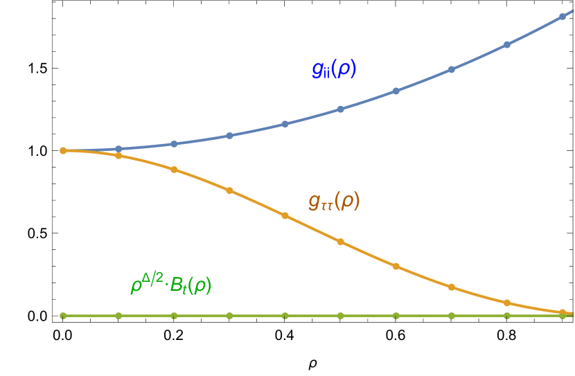
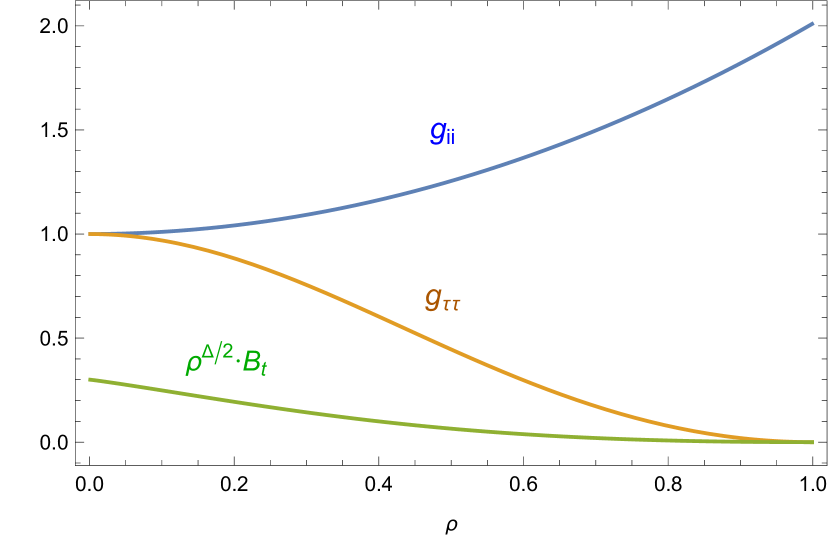
It is possible to find an analytic solution of the background for the case with . This is given by
| (7) |
We display in Fig. 1 (left) the numerical solution of the equations of motion for (dots), and compare it with the corresponding analytical solution (solid lines). We display also in the right panel the numerical solution for .
3 Anomalous conductivity
To compute these correlators, we will follow the general procedure of the perturbation of the fields on top of the background, and later use the AdS/CFT dictionary to compute the correlators.
3.1 Fluctuations
Within this approach, we perturb the fields on top of the numerical solution for the background displayed in Fig. 1. We will study the linear response of the fluctuations by splitting the metric and gauge field into background and linear perturbation components, i.e.
| (8) |
where the terms with (0) correspond to the background metric/field, and the terms with the fluctuations of this metric/field. Then, we will follow the general procedure of Fourier mode decomposition Amado:2011zx
| (9) | |||||
| (10) |
Without loss of generality, we consider perturbations with frequency and momentum in the -direction. Since we aim to compute correlators at zero frequency, we set the frequency-dependent parts to zero in the equations and solve the system up to first order in . In this limit, the fields decouple from the system and become constant. Thus, we can write the system of differential equations for the shear sector as follows
| (11) | |||
| (12) |
where . The explicit expressions of the functions and are given in Appendix A of Rai:2023nxe .
The asymptotic behaviour of the fields up to the first subleading term are given by
| (13) | |||||
| (14) |
where the leading-order terms and play the role of sources.
Conductivities
From the holographic description of the correlation functions, one can evaluate the one-point functions as
| (15) |
with . is the renormalized action, with the action given in Eq. (3) and the counterterm. The two-point functions can be obtained by taking the variation of one-point function with respect to the corresponding source term and the conductivities are evaluated using the Kubo formulae given in (1) and (2), i.e.
| (16) | ||||
| (17) |
A comparison of the variation of the action under axial gauge transformations with the consistent form of the anomaly for chiral fermions book1 allows us to set the value of the anomaly coefficients to
| (18) |
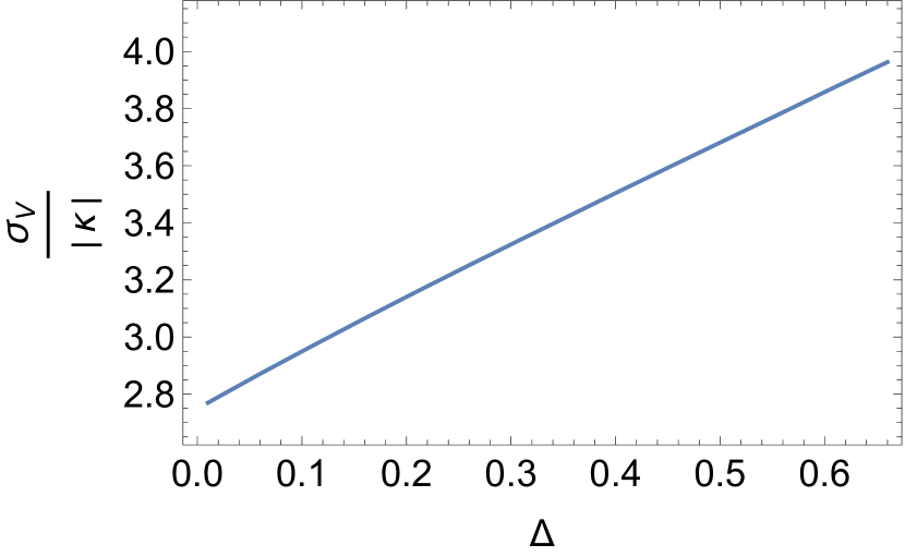
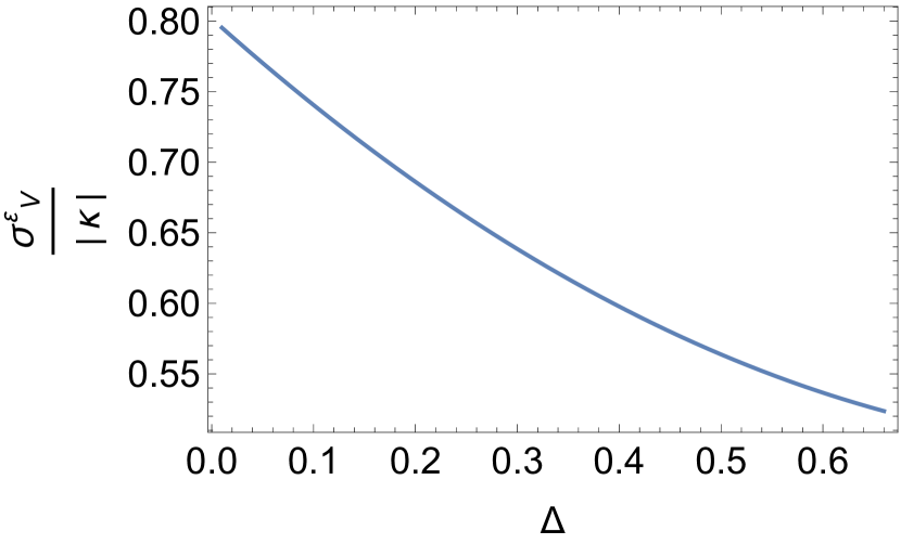
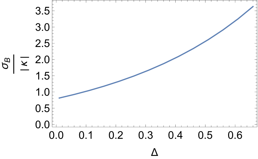
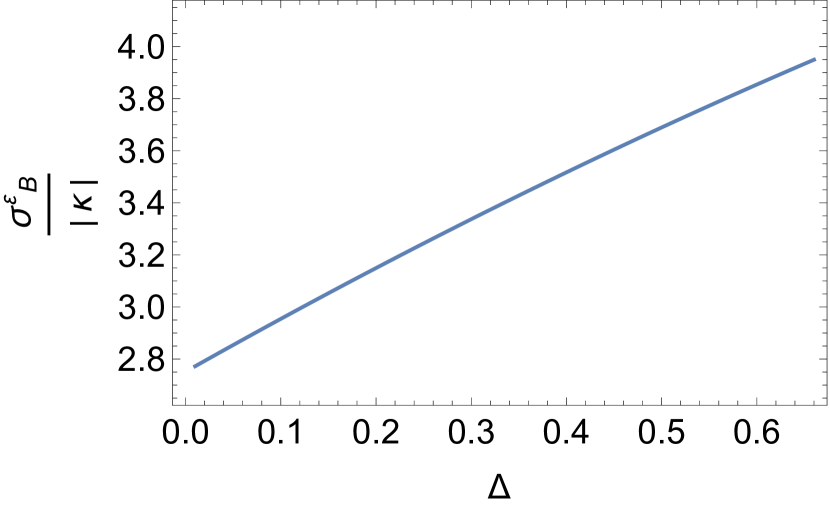
In this regard we will be setting , so that and . In Fig. 2 we have plotted the anomalous conductivities vs (a parameter related to the mass of the gauge field). From this figure, we observe that the chiral vortical conductivity and the chiral magnetic conductivity for energy current are the same even at finite mass, i.e., , and both increase with . Additionally, we see that the chiral vortical conductivity of energy current, , decreases with , but the rate decreases rapidly. Conversely, in the case of the chiral magnetic conductivity, , it increases with as shown in Fig. 2. In the limit of vanishing mass, our results lead to , which exactly coincides with the results in Landsteiner:2011iq ; Jimenez-Alba:2014iia where has been set to in both references 111 corresponds to the asymptotic value of the gauge field for . In our case, we assume for ..
4 Discussion
In this work we have studied the mass dependence of the anomalous conductivities in a holographic model for a massive gauge field, incorporating both pure gauge and mixed gauge-gravitational anomaly terms. In this model, the vortical sector was also accessible, and the conductivities corresponding to this sector were also studied. We observed that the chiral vortical conductivity, , and the chiral magnetic conductivity for energy current, , are equal and increase with . An intriguing finding is the presence of contributions to induced by the mixed gauge-gravitational anomaly term in the massive theory, which were absent in the massless case. Furthermore, the conductivities , , and all increase with , while the chiral vortical conductivity of energy current, , decreases with . We have explicitly verified that all our numerical results for the conductivities at finite mass converge to the known results at zero mass as .
Acknowledgments
N.R. thanks the International Centre for Theoretical Sciences (ICTS) for the support through the program - Field Theory and Turbulence (ICTS/FTT2023/12). The works of N.R. and E.M. are supported by the project PID2020-114767GB-I00 and by the Ramón y Cajal Program under Grant RYC-2016-20678 funded by MCIN/AEI/10.13039/501100011033 and by “FSE Investing in your future”, as well as by the FEDER/Junta de Andalucía-Consejería de Economía y Conocimiento 2014–2020 Operational Program under Grant A-FQM-178-UGR18. The work of E.M. is also supported by Junta de Andalucía under Grant FQM-225, and by the “Prórrogas de Contratos Ramón y Cajal” Program of the University of Granada.
References
- (1) J. M. Maldacena, Int. J. Theor. Phys. 38, 1113 (1999) [Adv. Theor. Math. Phys. 2, 231 (1998)] doi:10.1023/A:1026654312961 [hep-th/9711200].
- (2) E. Witten, Adv. Theor. Math. Phys. 2, 253 (1998) [hep-th/9802150].
- (3) S. Grieninger and S. Morales-Tejera, Phys. Rev. D 108 (2023) no.12, 126010 doi:10.1103/PhysRevD.108.126010 [arXiv:2308.14829 [hep-ph]].
- (4) M. Baggioli, Y. Bu and V. Ziogas, JHEP 09 (2023), 019 doi:10.1007/JHEP09(2023)019 [arXiv:2304.14173 [hep-th]].
- (5) S. Morales-Tejera, V. E. Ambruş and M. N. Chernodub, [arXiv:2403.19755 [hep-th]].
- (6) K. Landsteiner, S. Morales-Tejera and P. Saura-Bastida, Phys. Rev. D 107 (2023) no.12, 125003 doi:10.1103/PhysRevD.107.125003 [arXiv:2212.14088 [hep-th]].
- (7) N. Rai and E. Megías, JHEP 06 (2023), 215 doi:10.1007/JHEP06(2023)215 [arXiv:2301.00361 [hep-th]].
- (8) S. Mukhopadhyay and N. Rai, JHEP 09 (2021), 160 doi:10.1007/JHEP09(2021)160 [arXiv:2008.00432 [hep-th]].
- (9) N. Rai, Eur. Phys. J. C 79 (2019) no.11, 972 doi:10.1140/epjc/s10052-019-7469-x
- (10) S. Mukhopadhyay and N. Rai, Phys. Rev. D 96 (2017) no.6, 066001 doi:10.1103/PhysRevD.96.066001
- (11) S. Mukhopadhyay and N. Rai, Phys. Rev. D 96 (2017) no.2, 026005 doi:10.1103/PhysRevD.96.026005
- (12) M. Ammon, D. Arean, M. Baggioli, S. Gray and S. Grieninger, JHEP 03 (2022), 015 doi:10.1007/JHEP03(2022)015 [arXiv:2111.10305 [hep-th]].
- (13) S. Grieninger and S. Morales-Tejera, EPJ Web Conf. 258 (2022), 10007 doi:10.1051/epjconf/202225810007 [arXiv:2111.14116 [hep-ph]].
- (14) Y. Ahn, M. Baggioli, Y. Liu and X. M. Wu, JHEP 03 (2024), 124 doi:10.1007/JHEP03(2024)124 [arXiv:2401.07772 [hep-th]].
- (15) H. Chu, X. Ji and Y. W. Sun, JHEP 05 (2024), 166 doi:10.1007/JHEP05(2024)166 [arXiv:2403.02669 [hep-th]].
- (16) K. Landsteiner and Y. Liu, Phys. Lett. B 753 (2016), 453-457 doi:10.1016/j.physletb.2015.12.052 [arXiv:1505.04772 [hep-th]].
- (17) K. Landsteiner and L. Melgar, JHEP 10 (2012), 131 doi:10.1007/JHEP10(2012)131 [arXiv:1206.4440 [hep-th]].
- (18) E. Megías and F. Pena-Benitez, JHEP 05, 115 (2013) doi:10.1007/JHEP05(2013)115 [arXiv:1304.5529 [hep-th]].
- (19) G. M. Newman and D. T. Son, Phys. Rev. D 73 (2006), 045006 doi:10.1103/PhysRevD.73.045006 [arXiv:hep-ph/0510049 [hep-ph]].
- (20) G. M. Newman, JHEP 01 (2006), 158 doi:10.1088/1126-6708/2006/01/158 [arXiv:hep-ph/0511236 [hep-ph]].
- (21) E. Megías, EPJ Web Conf. 164 (2017), 08001 doi:10.1051/epjconf/201716408001 [arXiv:1701.00087 [hep-th]].
- (22) K. Landsteiner, E. Megías and F. Pena-Benitez, Phys. Rev. D 90, no.6, 065026 (2014) doi:10.1103/PhysRevD.90.065026 [arXiv:1312.1204 [hep-ph]].
- (23) R. A. Bertlmann, Oxford, UK: Clarendon (1996) 566 p. (International series of monographs on physics: 91).
- (24) F. Bastianelli and P. van Nieuwenhuizen, Cambridge,UK: Univ. Pr. (2006) 379p.
- (25) K. Fujikawa and H. Suzuki, Oxford,UK: Clarendon (2004) 284p.
- (26) K. Landsteiner, E. Megías and F. Pena-Benitez, Lect. Notes Phys. 871 (2013), 433-468 doi:10.1007/978-3-642-37305-3_17 [arXiv:1207.5808 [hep-th]].
- (27) A. Vilenkin, Phys. Rev. D20 (1979) 1807. A. Vilenkin, Phys. Rev. D21 (1980) 2260. A. Vilenkin, Phys. Rev. D22 (1980) 3067. A. Vilenkin, Phys. Rev. D22 (1980) 3080.
- (28) K. Fukushima, D. E. Kharzeev and H. J. Warringa, Phys. Rev. D 78 (2008), 074033 doi:10.1103/PhysRevD.78.074033 [arXiv:0808.3382 [hep-ph]].
- (29) D. Kharzeev and A. Zhitnitsky, Nucl. Phys. A 797 (2007), 67-79 doi:10.1016/j.nuclphysa.2007.10.001 [arXiv:0706.1026 [hep-ph]].
- (30) N. Banerjee, J. Bhattacharya, S. Bhattacharyya, S. Dutta, R. Loganayagam and P. Surowka, JHEP 01 (2011), 094 doi:10.1007/JHEP01(2011)094 [arXiv:0809.2596 [hep-th]].
- (31) D. T. Son and P. Surowka, Phys. Rev. Lett. 103 (2009), 191601 doi:10.1103/PhysRevLett.103.191601 [arXiv:0906.5044 [hep-th]].
- (32) K. Landsteiner, E. Megías and F. Pena-Benitez, Phys. Rev. Lett. 107, 021601 (2011) doi:10.1103/PhysRevLett.107.021601 [arXiv:1103.5006 [hep-ph]].
- (33) B. I. Abelev et al. [STAR], Phys. Rev. Lett. 103 (2009), 251601 doi:10.1103/PhysRevLett.103.251601 [arXiv:0909.1739 [nucl-ex]].
- (34) G. Basar, D. E. Kharzeev and H. U. Yee, Phys. Rev. B 89, no.3, 035142 (2014) doi:10.1103/PhysRevB.89.035142 [arXiv:1305.6338 [hep-th]].
- (35) K. Landsteiner, Phys. Rev. B 89, no.7, 075124 (2014) doi:10.1103/PhysRevB.89.075124 [arXiv:1306.4932 [hep-th]].
- (36) K. Landsteiner, E. Megías, L. Melgar and F. Pena-Benitez, JHEP 09 (2011), 121 doi:10.1007/JHEP09(2011)121 [arXiv:1107.0368 [hep-th]].
- (37) D. T. Son and A. O. Starinets, JHEP 09 (2002), 042 doi:10.1088/1126-6708/2002/09/042 [arXiv:hep-th/0205051 [hep-th]].
- (38) C. P. Herzog and D. T. Son, JHEP 03 (2003), 046 doi:10.1088/1126-6708/2003/03/046 [arXiv:hep-th/0212072 [hep-th]].
- (39) A. Jimenez-Alba, K. Landsteiner and L. Melgar, Phys. Rev. D 90 (2014), 126004 doi:10.1103/PhysRevD.90.126004 [arXiv:1407.8162 [hep-th]].
- (40) I. R. Klebanov, P. Ouyang and E. Witten, Phys. Rev. D 65 (2002), 105007 doi:10.1103/PhysRevD.65.105007 [arXiv:hep-th/0202056 [hep-th]].
- (41) U. Gürsoy and A. Jansen, JHEP 10 (2014), 092 doi:10.1007/JHEP10(2014)092 [arXiv:1407.3282 [hep-th]].
- (42) R. Casero, E. Kiritsis and A. Paredes, Nucl. Phys. B 787 (2007), 98-134 doi:10.1016/j.nuclphysb.2007.07.009 [arXiv:hep-th/0702155 [hep-th]].
- (43) E. Megías and M. Valle, Fortsch. Phys. 66, no.7, 1800035 (2018) doi:10.1002/prop.201800035 [arXiv:1707.04747 [hep-th]].
- (44) E. Megías, J. Phys. Conf. Ser. 1416, no.1, 012022 (2019) doi:10.1088/1742-6596/1416/1/012022 [arXiv:1909.13836 [hep-th]].
- (45) I. Amado, K. Landsteiner and F. Pena-Benitez, JHEP 05 (2011), 081 doi:10.1007/JHEP05(2011)081 [arXiv:1102.4577 [hep-th]].
- (46) A. Gynther, K. Landsteiner, F. Pena-Benitez and A. Rebhan, JHEP 02 (2011), 110 doi:10.1007/JHEP02(2011)110 [arXiv:1005.2587 [hep-th]].