High Throughput Polar Code Decoders with Information Bottleneck Quantization

Abstract

In digital baseband processing, the forward error correction (FEC) unit belongs to the most demanding components in terms of computational complexity and power consumption. Hence, efficient implementation of FEC decoders is crucial for next generation mobile broadband standards and an ongoing research topic. Quantization has a significant impact on the decoder area, power consumption and throughput. Thus, lower bit-widths are preferred for efficient implementations but degrade the error-correction capability. To address this issue, a non-uniform quantization based on the Information Bottleneck (IB) method, was proposed that enables a low bit width while maintaining the essential information. Many investigations on the use of IB method for Low-density parity-check code (LDPC) decoders exist and have shown its advantages from an implementation perspective. However, for polar code decoder implementations, there exists only one publication that is not based on the state-of-the-art Fast-SSC decoding algorithm, and only synthesis implementation results without energy estimation are shown. In contrast, our paper presents several optimized Fast Simplified Successive-Cancellation (Fast-SSC) polar code decoder implementations using IB-based quantization with placement&routing results in an advanced 12 nm FinFET technology. Gains of up to 16 % in area and 13 % in energy efficiency are achieved with IB-based quantization at a Frame Error Rate (FER) of $10^{-7}$ and a Polar Code of $N=1024,R=0.5$ compared to state-of-the-art decoders.

I Introduction

Polar codes are a relatively new class of Forward Error Correction (FEC) codes, first described by Erdal Arıkan in 2009 [1]. These codes are part of the 5G standard. They offer low-complexity encoding and decoding algorithms, which is especially important for high-throughput and low-latency applications in upcoming standards such as 6G [2]. The most commonly used decoding algorithms for polar codes, Successive Cancellation (SC) and Successive Cancellation List (SCL), can be efficiently pipelined to achieve very high throughput and low latency [3, 4].

Quantization has a significant impact on implementation costs. Coarse quantization improves implementation efficiency in terms of area, power and throughput but may decrease the error-correction performance. Finding a good trade-off is therefore essential for efficient hardware implementations.

One promising technique to maintain the message information but enable a reduction of the bit width is the Information Bottleneck (IB) method [5]. Here, an information compression is achieved by maximizing the mutual information between an observed and a compressed random variable for a given bit width. This yields a non-uniform quantization.

While IB-based quantization for Low Density Parity Check (LDPC) decoder implementations is well investigated [6, 7, 8], the efficiency of the IB method for polar code decoder is quite unexplored. It is an open research question whether IB based quantization in polar decoders can yield more efficient implementations compared to standard quantization methods. It was shown in [8, 9], that a pure lookup table (LUT)-based application of the IB method yields very large LUTs, making this approach unfeasible. The Reconstruction Computation Quantization (RCQ) scheme [10] also uses LUTs to reconstruct and, after computation, quantize back to smaller bit width. The resulting LUTs have much lower complexity. Hence, the RCQ scheme is the most promising approach from an implementation perspective.

To the best of our knowledge, only one publication investigates the efficiency of IB-based polar decoder implementation [9]. However, the investigations in [9] do not consider the state-of-the-art Fast Simplified Successive Cancellation (Fast-SSC) decoding algorithm and, even more importantly, provides only synthesis results without any power data, which is one of the most important implementation metrics.

This work therefore makes the following new contributions:

• We present the first Fast-SSC polar decoder architecture using IB-based quantization with optimized LUTs to improve area and energy efficiency.

• We compare the non-uniform, IB-based quantization scheme with uniformly quantized fixed-point (FP) representations in terms of error correction performance and implementation efficiency for code lengths of $128\text{\,}\mathrm{bit}\text{/}$ and $1024\text{\,}\mathrm{bit}\text{/}$.

• We analyse the impact of the IB-based quantization on area and power consumption with 7 different designs in an advanced $12\text{\,}\mathrm{nm}\text{/}$ FinFET technology.

The remainder of this paper is structured as follows: We provide the required background of polar codes, their decoding algorithms and the IB method in Sec. II. IB-based Fast-SSC decoding and our decoder architecture is described in Sec. III. Sec. IV presents a detailed comparison with uniformly quantized FP decoders in terms of error correction performance and implementation costs and Sec. V concludes this paper.

II Background

II-A Polar Codes

Polar codes $\mathcal{P}(N,K)$ are linear block codes with code length $N=2^{n}$, that encode $K$ information bits. Channel polarization derives $N$ virtual channels where $K$ reliable channels (information set $\mathcal{I}$) are used to transmit the information. The $N-K$ remaining (unreliable) channels are set to zero and called frozen bits (frozen set $\mathcal{F}$). The encoding includes a bit-reversal permutation [1].

II-B Successive Cancellation Decoding

SC decoding can be described as depth-first tree traversal of the Polar Factor Tree (PFT) [11]. The PFT has ${\log(N)+1}$ stages $s$ and $N$ leaf nodes at stage $s=0$, representing the frozen and information bits. Each node $v$ receives a Log-Likelihood Ratio (LLR) vector $\boldsymbol{\alpha}^{v}$ of size $N_{s}$ to first calculate the $N_{s}/2$ elements of the left-child message $\boldsymbol{\alpha}^{l}$ by the hardware-efficient min-sum formulation of the $f$-function

$$\alpha^{l}_{i} =f(\alpha^{v}_{2i},\alpha^{v}_{2i+1})$$ (1)

$$=\operatorname{sign}\left(\alpha^{v}_{2i}\right)\operatorname{sign}\left(\alpha^{v}_{2i+1}\right)\min\left(\left|\alpha^{v}_{2i}\right|,\left|\alpha^{v}_{2i+1}\right|\right).$$

With the bit vector $\boldsymbol{\beta}^{l}$ received from the left child, the $N_{s}/2$ elements of $\boldsymbol{\alpha}^{r}$ are calculated using the $g$-function

$$\alpha^{r}_{i}=g\left(\alpha^{v}_{2i},\alpha^{v}_{2i+1},\beta^{l}_{i}\right)=\left(1-2\beta^{l}_{i}\right)\cdot\alpha^{v}_{2i}+\alpha^{v}_{2i+1},$$ (2)

and sent to the child on the right. With the results of both children, the $h$-function calculates the partial-sum $\boldsymbol{\beta}^{v}$ with $\oplus$, the binary XOR-operator, as

$$\left(\beta^{v}_{2i},\beta^{v}_{2i+1}\right)=h\left(\beta^{l}_{i},\beta^{r}_{i}\right)=\left(\beta^{l}_{i}\oplus\beta^{r}_{i},\beta^{r}_{i}\right),$$ (3)

that is sent to the parent node. In leaf nodes, bit decisions are made. Frozen bits are $0$ per definition, and information bit nodes return the Hard Decision (HD) on the LLR:

$$\beta^{v}=\operatorname{sign}\left(\alpha^{v}\right)\triangleq\begin{cases}0&\text{if }\alpha^{v}\geq 0\\ 1&\text{otherwise.}\end{cases}$$ (4)

The decoder outputs the partial-sum $\boldsymbol{\beta}^{0}$ of the root node.

II-C Fast-SSC Decoding

Pruning the PFT reduces the number of operations required to decode one code word [11]. Subtrees containing only frozen bits do not have to be traversed, because their decoding result is known to be an all-zero vector in advance. Such Rate-0 nodes are always left children and are merged into their parent nodes. Here, the $g$- and $h$-functions are executed with the known all-zero $\boldsymbol{\beta}^{l}$, denoted by $g_{0}$ and $h_{0}$, respectively. Similarly, subtrees without any frozen bits can be decoded directly by the HD, because no parity information is contained. Merging these Rate-1 nodes results in the $h_{1}$-function, which directly calculates $\boldsymbol{\beta}^{r}$ using

$$\beta^{r}_{i}=\operatorname{sign}\left(g\left(\alpha^{v}_{2i},\alpha^{v}_{2i+1},\beta^{l}_{i}\right)\right),$$ (5)

and combines it with $\boldsymbol{\beta}^{l}$ to observe $\boldsymbol{\beta}^{v}$.

Fast-SSC decoding [12] applies further optimizations: If a subtree contains only one information bit, it is considered a Repetition (REP) code and replaced by a specialized REP node. All its bits are decoded by summing up the vector $\alpha^{v}$ of received LLR values and extracting the sign bit of the sum:

$$\beta^{v,\text{REP}}_{i}=\operatorname{sign}\left(\sum_{j=0}^{N_{s}-1}\alpha^{v}_{j}\right).$$ (6)

In subtrees containing only one frozen bit, this bit always acts as parity bit. Thus, the partial sum of this subtree represents a Single Parity-Check (SPC) code. A specialized SPC node performs Maximum Likelihood (ML) decoding by calculating the parity $\gamma^{v}\in\{0,1\}$ of the input:

$$\gamma^{v}=\bigoplus_{i=0}^{N_{s}-1}\operatorname{sign}\left(\alpha^{v}_{i}\right),$$ (7)

finding the least reliable bit

$$i_{\min}=\operatorname*{arg\,min}_{i\in[0,N_{s})}\left|\alpha^{v}_{i}\right|$$ (8)

and setting $\boldsymbol{\beta}^{v}$ to satisfy the single parity constraint:

$$\beta^{v,\text{SPC}}_{i}=\begin{cases}\operatorname{sign}\alpha^{v}_{i}\oplus\gamma^{v}&\text{if }i=i_{\min}\\ \operatorname{sign}\alpha^{v}_{i}&\text{otherwise.}\end{cases}$$ (9)

II-D Information Bottleneck Method

The IB method is a mathematical framework used for clustering in information theory and machine learning [5]. In the IB setup, the target is to preserve the shared mutual information $I(X;Y)$ between an observed random variable $Y$ and the relevant random variable $X$ while compressing $Y$ to $T$, i. e., maximizing $I(T;X)$. Different IB algorithms exist [13] to provide the compression mapping $p(t|y)$ derived only from the joint distribution $p(x;y)$ and the cardinality of the compressed event space ($|\mathcal{T}|$), with $x\in\mathcal{X}=\{0,1\},y\in\mathcal{Y},t\in\mathcal{T}$ being realizations of the random variables $X,Y,T$, respectively and $|\mathcal{T}|\ll|\mathcal{Y}|$. A collection of IB algorithms is provided by [14] and is used in this work. This compression is applied to the output of an Additive White Gaussian Noise (AWGN) channel to obtain a coarse, non-uniform quantization.

In the case of our IB decoder, $y\in\mathcal{Y}$ are the received LLRs that are quantized with a high bit width, e.g. $10\text{\,}\mathrm{b}\mathrm{i}\mathrm{t}$, which equals $|\mathcal{Y}|=2^{10}=1024$ bins. The IB algorithm then iteratively tries to find pairs of bins to combine into one bin with the least loss of mutual information $I(X;Y)$. In that way $|\mathcal{Y}|$ is reduced to $|\mathcal{T}|=16$ ($4\text{\,}\mathrm{b}\mathrm{i}\mathrm{t}$) and a mapping from $y$ to $t$ is derived.

III IB Decoder

III-A Numerical Representations and LUT Generation

In this paper, we focus on decoders with very high throughput and low latency. These decoders are fully unrolled and pipelined and use a Sign-Magnitude (SM) representation of the quantized, FP LLR values [15]. For high Signal-to-Noise-Ratios (SNRs), saturation reduces signal toggling because only the sign bit changes, which reduces power consumption. Additionally, the comparators in the $f$-functions (1) and SPC nodes (8) can directly operate on the magnitude. To perform the additions in the $g$-functions (2) and REP nodes (6), the SM representations are converted to Two’s-Complement (TC) to efficiently perform the calculations.

Our IB decoder implementations exploit all these optimizations. However, because of the non-uniform distribution characterizing the IB indices, mathematical computations must be replaced by LUTs [9]. However, these LUTs can become extremely large. For example, for a $g$-function (2) with one binary and two LLR inputs, the resulting LUT is of size $2\cdot|\mathcal{T}|^{2}$. From an implementation perspective, the LUTs are transformed into Boolean functions. Despite the logic optimization executed by state-of-the-art synthesis tools, the resulting logic costs can quickly outweigh the benefits of reduced bit widths, particularly for increasing LUT sizes [8].

A promising approach to address this problem is the RCQ scheme [10, 16]. RCQ combines non-uniform quantization with the traditional node computations. Only small LUTs are necessary that are placed in front of the computation units to upscale the reduced non-uniform IB quantization to a uniform FP quantization (Reconstruction). Node computations are then performed on the uniform FP quantization (Computation). After computation the results are downscaled to smaller bit width (Quantization). The RCQ scheme results in much smaller LUTs because the mappings for the conversions between IB and FP domains can be implemented as LUTs of size $2^{Q}$ for each value where $Q$ is the bit width. We use $Q_{\text{IB}}=\log_{2}(|\mathcal{T}|)$ and $Q_{\text{FP}}$ to denote the bit widths in the IB and FP domains, respectively. For the $g$-function example mentioned above, the number of entries in the LUTs shrinks from $2\cdot|\mathcal{T}|^{2}=2^{1+2\cdot Q_{\text{IB}}}$ to $2\cdot 2^{Q_{\text{IB}}}+2^{Q_{\text{FP}}}$.

TABLE I: Hardware-aware representation of $3\text{\,}\mathrm{bit}\text{/}$ IB indices

IB Index $t$	0	1	2	3	4	5	6	7
SM IB	-3	-2	-1	-0	0	1	2	3
Binary	1 11	1 10	1 01	1 00	0 00	0 01	0 10	0 11

We use density evolution to generate samples. At least 100K samples are monitored at each node in the decoder, i. e., at each edge of the PFT. These samples yield the joint distributions $p(x;y)$ which are input to the IB algorithm [13] that calculates the compression mappings $p(t|y)$ for every edge. Then, the Symmetric information bottleneck algorithm [7, 14] is applied which is optimized to preserve the symmetry of the transmission channel (assuming an AWGN channel and Binary Phase Shift Keying (BPSK) modulation). Exploiting this symmetry enables a bisection of the LUT , because it is sufficient to store only the magnitudes. Accordingly, we use a SM-like representation of the IB indices as shown in the example in Table I for $|\mathcal{T}|=8$. Therefore, for both directions of conversion (IB to FP, and FP to IB), the LUTs directly map one magnitude to another, i. e., the magnitudes in both domains also act as indices for the LUTs. Thus, the size of each LUT is $2^{Q-1}$ and the total number of entries for the example of the $g$-function becomes $2\cdot 2^{Q_{\text{IB}}-1}+2^{Q_{\text{FP}}-1}$. As shown in Figure 1 this means a reduction from $2*16^{2}=512$ entries to $2*2^{4-1}$ for the upscaling LUT and $2^{5-1}$ for the downscaling LUT, making it just 32 entries.

Furthermore, this approach eliminates the need for multiple comparisons with thresholds per conversion as in [16].

Notation

To differentiate between the numerical representations, we use $\alpha$ to denote values in the IB domain, $\tilde{\alpha}$ for SM and $\ddot{\alpha}$ for TC representation. The $j$-th bit of the binary expansion of $\alpha_{i}$ is given by $\alpha_{i_{(j)}}$ and the most significant bit (MSB) $Q-1$ refers to the sign bit.

III-B IB-based Fast-SSC Decoding

III-B1 $f$-Function

With the symmetric mapping and inherent order of the IB indices (Table I), the $f$-function (1) can be directly performed in the non-uniform IB domain and no LUTs are necessary, which corresponds to the “re-MS-IB decoder” implementation of [9]. In contrast to [9], we map the IB indices so that negative values also correspond to negative LLRs and, thus, do not need to invert the result of the XOR-ed sign bits.

III-B2 $g$-Function

Figure 1: RCQ schematic for the $g$-function

As in [16], we apply an RCQ scheme, but based on our optimized up- and downscale LUTs:

$$\alpha^{r}_{i}=\mathrm{LUT}^{v}_{\text{down}}\left(g\left(\mathrm{LUT}^{v}_{\text{up}}\left(\alpha^{v}_{2i}\right),\mathrm{LUT}^{v}_{\text{up}}\left(\alpha^{v}_{2i+1}\right),\beta^{l}_{i}\right)\right).$$ (10)

The internal separation between the different number representations is maintained for the reasons described in Sec. III-A and shown in Fig. 1. The Reconstruction with $\mathrm{LUT}^{v}_{\text{up}}$ maps the magnitude of the IB index $\alpha^{v}_{i}$ to its SM representation $\tilde{\alpha}^{v}_{i}$ with preserved sign bit. $\beta^{l}_{i}$ must be considered before conversion to the TC representation $\ddot{\alpha}^{v}_{i}$ for the Computation step. The result $\ddot{\alpha}^{r}_{i}$ has a $1\text{\,}\mathrm{bit}\text{/}$ larger resolution, implying a saturation for the conversion back to SM representation with $Q_{\text{FP}}\text{\,}\mathrm{bit}\text{/}$. The Quantization step is again realized as magnitude $\mathrm{LUT}^{v}_{\text{down}}$ for the transformation back to the IB domain.

For the special case of merged Rate-0 nodes, i. e., the $g_{0}$-function, the XOR-operation with $\beta^{v}_{i}$ is omitted.

III-B3 REP Nodes

REP nodes calculate the sum over all input values to observe the single (repeated) information bit by HD on the sum (6). Thus, the RCQ scheme as described for the $g$-function is applied for REP nodes. An adder tree of $N_{s}-1$ adders and a depth of $s=\log_{2}N_{s}$ operates on the TC representations of the $N_{s}$ input values. The final HD as Quantization step extracts the single sign bit as bit decision of the node, for which reason no further conversion of the sum is needed.

III-B4 SPC Nodes

As in the f-function, due to the ordered mapping of the IB indices, the minimum search of the SPC node (8) can be performed directly in the IB domain. Furthermore, the chosen mapping is also suitable for the direct parity calculation (7) and the bit estimations (9), because the sign bits are preserved in the IB domain.

III-B5 $h_{1}$-Function

The $h_{1}$-function internally uses the $g$-function to compute $\beta^{r}$ (5). However, in this $g$-function, the backward conversion is not needed, because the HD is made directly in the compute domain with TC representation, as already described for the REP nodes.

III-C Decoder Architecture

Figure 2: Unrolled and pipelined Fast-SSC decoder architecture for a $\mathcal{P}(16,8)$. Colors represent numerical domains: green for IB, red for FP, blue for binary and dark green shows the LUTs.

An outline of the fully unrolled and deeply pipelined Fast-Simplified SC (SSC) decoder architecture for a $\mathcal{P}(16,8)$ is shown in Figure  2. We omit the clock signals and the delay lines are represented by shift registers. The pipeline consists of various building blocks that implements the decoding functions described in the previous section. The IB, FP and binary domains are represented by the coloring of the blocks and signals. The decoders presented in this paper are based on the framework presented in [15] which we extended to apply the IB method as described above.

IV Results

We present 7 decoder designs for $N\!=\!128$ and $N\!=\!1024$ which are optimized for a target frequency of $500\text{\,}\mathrm{MHz}\text{/}$ and $750\text{\,}\mathrm{MHz}\text{/}$, respectively. Throughput is considered as coded throughput. The designs were synthesized with Design Compiler and placed and routed with IC-Compiler, both from Synopsys in a $12\text{\,}\mathrm{nm}\text{/}$ FinFET technology with a super-low $V_{t}$ transistor library from Global Foundries under worst case Process, Voltage and Temperature (PVT) conditions ($125\text{\,}\mathrm{\SIUnitSymbolCelsius}\text{/}$, $0.72\text{\,}\mathrm{V}\text{/}$) for timing and nominal case PVT ($25\text{\,}\mathrm{\SIUnitSymbolCelsius}\text{/}$, $0.8\text{\,}\mathrm{V}\text{/}$) for power. Error-correction performance was simulated for an AWGN channel and BPSK modulation with a minimum of 100 erroneous code words.

IV-A Decoder for the Polar(128,64) Code

The Frame Error Rate (FER) of the $\mathcal{P}(128,64)$ is shown in Figure 3. The IB decoder with $4\text{\,}\mathrm{bit}\text{/}$ and the FP decoder with $5\text{\,}\mathrm{bit}\text{/}$ show similar error-correction performance, whereas the error-correction performance of the $4\text{\,}\mathrm{bit}\text{/}$ FP decoder starts to degrade at an FER of $10^{-3}$.

TABLE II: Implementation results for $\mathcal{P}(128,64)$ decoders

	IB 4bit	[9]*	FP 4bit	FP 5bit
	Place&Route	Synthesis	Place&Route	Place&Route
Technology	$12\text{\,}\mathrm{nm}\text{/}$	$28\text{\,}\mathrm{nm}\text{/}$$\rightarrow$$12\text{\,}\mathrm{nm}\text{/}$	$12\text{\,}\mathrm{nm}\text{/}$	$12\text{\,}\mathrm{nm}\text{/}$
Frequency [MHz]	500	1000 (3681)	500	500
Throughput [Gbps]	64	13 (47)	64	64
Latency [ns]	18	86 (23)	18	18
Latency [CC]	9	86	9	9
Area [mm2]	0.014	0.026	0.012	0.015
- Registers	0.005	—	0.005	0.006
- Combinatorial	0.005	—	0.003	0.005
Area Eff. [Gbps/mm2]	4528	502 (1847)	5384	4248
Power Total [mW]	21	—	17	24
- Clock	7	—	7	9
- Registers	3	—	3	4
- Combinatorial	10	—	7	11
Energy Eff. [pJ/bit]	0.32	—	0.27	0.37
Power Density [W/mm2]	1.46	—	1.47	1.58

^* Synthesis only, scaled from $28\text{\,}\mathrm{nm}\text{/}$ to $12\text{\,}\mathrm{nm}\text{/}$ (numbers in brackets) with equations from [17] and maximum frequency limited to $1000\text{\,}\mathrm{MHz}\text{/}$. For $28\text{\,}\mathrm{nm}\text{/}$ and $12\text{\,}\mathrm{nm}\text{/}$ the scaling factors of $32\text{\,}\mathrm{nm}\text{/}$ and $14\text{\,}\mathrm{nm}\text{/}$ were used, since they belong to the same technology generation and give the best approximation.

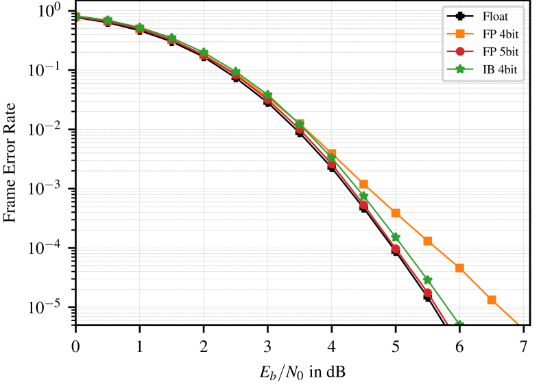
Figure 3: FER of the $\mathcal{P}(128,64)$, Float vs. FP vs. IB Quantization

Table II presents the corresponding implementation results. Comparing the decoders with similar FER (IB vs. $5\text{\,}\mathrm{bit}\text{/}$ FP), we observe similar combinatorial area (logic), whereas the area for the memory (registers) is reduced by ~$16\text{\,}\mathrm{\char 37\relax}\text{/}$. This improves the area efficiency by ~$7\text{\,}\mathrm{\char 37\relax}\text{/}$ and yields power savings and energy efficiency improvements of ~$13\text{\,}\mathrm{\char 37\relax}\text{/}$.

When comparing the IB decoder with the $4\text{\,}\mathrm{bit}\text{/}$ FP decoder, the cost of the LUTs can be directly observed in the combinatorial area (0.005 mm² vs. 0.003mm²) while the area for the registers is identical. This cost can be considered as the price for the improved error correction performance of the IB decoder.

As already mentioned there exits only one other publication that gives implementation results for IB-based decoders. Since the authors of [9] only provide synthesis results in an older $28\text{\,}\mathrm{nm}\text{/}$ technology, a fair comparison is difficult. To enable at least some comparison, we scaled the results of [9] to $12\text{\,}\mathrm{nm}\text{/}$ according to the equations of [17]. The scaled results are included in Table II. We limited the maximum frequency to $1000\text{\,}\mathrm{MHz}\text{/}$ which is more reasonable, since $3681\text{\,}\mathrm{MHz}\text{/}$ (and even $1510\text{\,}\mathrm{MHz}\text{/}$ in the original publication) are not realistic for a design in $28\text{\,}\mathrm{nm}\text{/}$ after placement. The reasons are: first, the power consumption and power density becomes infeasible with this high frequency. Second, $3681\text{\,}\mathrm{MHz}\text{/}$ are unfeasible for standard placement and routing in semi-custom design flows in $28\text{\,}\mathrm{nm}\text{/}$ technology. Even with the scaled estimate without frequency limitation, we observe that our optimised decoders outperform [9] in throughput, latency, area and area efficiency.

IV-B Decoder for the Polar(1024,512) Code

The longer $\mathcal{P}(1024,512)$ polar code has a longer pipeline and is therefore more affected by accumulating quantization errors. In contrast to the shorter code, $6\text{\,}\mathrm{bit}\text{/}$ FP are necessary to match the floating point precision. We compare the $4\text{\,}\mathrm{bit}\text{/}$ IB decoder to the FP decoder with $5\text{\,}\mathrm{bit}\text{/}$, as they show similar error-correction performance (Figure 4). Here, the IB decoder even outperforms the $5\text{\,}\mathrm{bit}\text{/}$ FP decoder at an FER of $10^{-7}$.

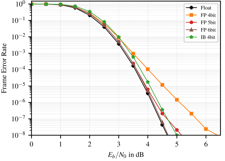
Figure 4: FER of the $\mathcal{P}(1024,512)$, Float vs. FP vs. IB 

TABLE III: Implementation results for $\mathcal{P}(1024,512)$ decoders

	IB 4bit	FP 4bit	FP 5bit	FP 6bit
Frequency [MHz]	750	750	750	750
Throughput [Gbps]	768	768	768	768
Latency [CC]	92	92	92	92
Area [mm2]	0.822	0.785	0.968	1.158
- Registers	0.360	0.360	0.439	0.517
- Combinatorial	0.200	0.168	0.208	0.274
Area Eff. [Gbps/mm2]	935	979	794	663
Power Total [W]	0.984	0.866	1.149	1.431
- Clock	0.208	0.207	0.254	0.298
- Registers	0.280	0.263	0.354	0.404
- Combinatorial	0.479	0.381	0.523	0.706
Energy Eff. [pJ/bit]	1.28	1.13	1.50	1.86
Power Density [W/mm2]	1.20	1.10	1.19	1.24

Comparing the implementation results of the IB decoder and the $5\text{\,}\mathrm{bit}\text{/}$ FP decoder (Table III), the total area is reduced by ~$15\text{\,}\mathrm{\char 37\relax}\text{/}$, mostly stemming from the reduction in registers. This leads to an improved area efficiency of ~$18\text{\,}\mathrm{\char 37\relax}\text{/}$, whereas the energy efficiency improves by ~$15\text{\,}\mathrm{\char 37\relax}\text{/}$. Figure 5 shows the layouts of the $5\text{\,}\mathrm{bit}\text{/}$ FP and the $4\text{\,}\mathrm{bit}\text{/}$ IB decoder. It is also worth noting that, when compared to the close-to-float $6\text{\,}\mathrm{bit}\text{/}$ FP decoder, accepting a small loss of ~$0.2\text{\,}\mathrm{dB}\text{/}$ in the error correction leads to improvements of ~$41\text{\,}\mathrm{\char 37\relax}\text{/}$ in area efficiency and ~$31\text{\,}\mathrm{\char 37\relax}\text{/}$ energy efficiency.

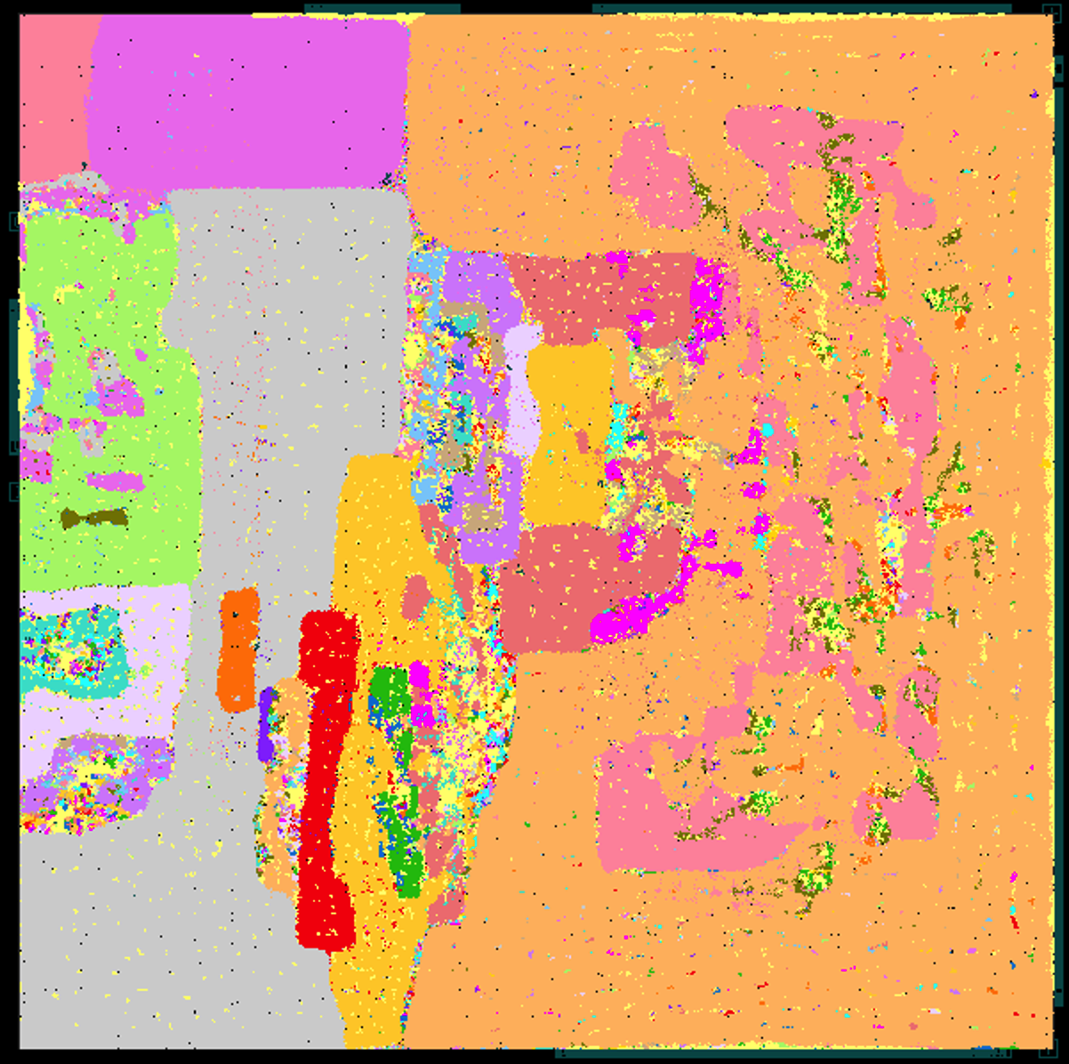
(a) FP $5\text{\,}\mathrm{bit}\text{/}$: $0.968\text{\,}{\mathrm{mm}}^{2}\text{/}$

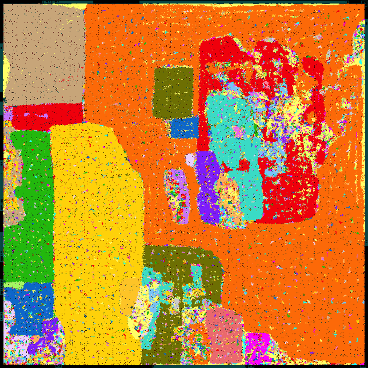
(b) IB $4\text{\,}\mathrm{bit}\text{/}$: $0.822\text{\,}{\mathrm{mm}}^{2}\text{/}$

Figure 5: Layout pictures for FP and IB polar code decoders

V Conclusion

We presented fully characterized Fast-SSC Polar Decoders with an optimized IB-based quantization scheme. Especially for ultra-high throughput we outperform decoders with comparable bit-width by $18\text{\,}\mathrm{\char 37\relax}\text{/}$ in area efficiency and $15\text{\,}\mathrm{\char 37\relax}\text{/}$ in energy efficiency. This effect can be explained by the savings in memory requirements of fully pipelined and unrolled decoders which is minimized with the IB-based quantization.

References

- [1] E. Arıkan, “Channel polarization: A method for constructing capacity-achieving codes for symmetric binary-input memoryless channels,” IEEE Trans. Inf. Theory, vol. 55, no. 7, pp. 3051–3073, 2009.
- [2] W. Saad, M. Bennis, and M. Chen, “A vision of 6G wireless systems: Applications, trends, technologies, and open research problems,” IEEE Network, vol. 34, no. 3, pp. 134–142, 2020.
- [3] A. Süral, E. G. Sezer, E. Kolagasioglu, V. Derudder, and K. Bertrand, “Tb/s polar successive cancellation decoder 16nm ASIC implementation,” CoRR, vol. abs/2009.09388, 2020. [Online]. Available: https://arxiv.org/abs/2009.09388
- [4] C. Kestel, L. Johannsen, O. Griebel, J. Jimenez, T. Vogt, T. Lehnigk-Emden, and N. Wehn, “A 506gbit/s polar successive cancellation list decoder with crc,” in 2020 IEEE 31st Annual International Symposium on Personal, Indoor and Mobile Radio Communications, Virtual Conference, Aug 2020, pp. 1–7.
- [5] N. Tishby, F. C. Pereira, and W. Bialek, “The information bottleneck method,” in Proc. of the 37-Th Annual Allerton Conference on Communication, Control and Computing, Monticello, IL, USA, 1999, pp. 368–377.
- [6] B. M. Kurkoski, K. Yamaguchi, and K. Kobayashi, “Noise Thresholds for Discrete LDPC Decoding Mappings,” in GLOBECOM 2008 - 2008 IEEE Global Telecommunications Conference, New Orleans, LA, USA, Nov 2008, pp. 1–5.
- [7] J. Lewandowsky and G. Bauch, “Information-optimum ldpc decoders based on the information bottleneck method,” IEEE Access, vol. 6, pp. 4054–4071, 2018.
- [8] T. Monsees, O. Griebel, M. Herrmann, D. Wübben, A. Dekorsy, and N. Wehn, “Minimum-integer computation finite alphabet message passing decoder: From theory to decoder implementations towards 1 tb/s,” Entropy, vol. 24, Article 1452, no. 10, 2022. [Online]. Available: https://www.mdpi.com/1099-4300/24/10/1452
- [9] P. Giard, S. A. A. Shah, A. Balatsoukas-Stimming, M. Stark, and G. Bauch, “Unrolled and pipelined decoders based on look-up tables for polar codes,” in 2023 12th International Symposium on Topics in Coding (ISTC), Brest, France, Sept 2023, pp. 1–5.
- [10] L. Wang, R. D. Wesel, M. Stark, and G. Bauch, “A Reconstruction-Computation-Quantization (RCQ) Approach to Node Operations in LDPC Decoding,” in GLOBECOM 2020 - 2020 IEEE Global Communications Conference. Taipei, Taiwan: IEEE, Dec 2020, pp. 1–6.
- [11] A. Alamdar-Yazdi and F. R. Kschischang, “A simplified successive-cancellation decoder for polar codes,” IEEE Commun. Lett., vol. 15, pp. 1378–1380, Dec 2011.
- [12] G. Sarkis, P. Giard, A. Vardy, C. Thibeault, and W. J. Gross, “Fast polar decoders: Algorithm and implementation,” IEEE J. Sel. Areas Commun., vol. 32, no. 5, pp. 946–957, may 2014.
- [13] N. Slonim, “The information bottleneck: Theory and applications,” http://www.yaroslavvb.com/papers/slonim-information.pdf, 2002.
- [14] M. Stark and J. Lewandowsky, “Information bottleneck algorithms in python,” {https://goo.gl/QjBTZf/}, 2018.
- [15] T. Lehnigk-Emden, M. Alles, C. Kestel, and N. Wehn, “Polar code decoder framework,” in 2019 Design, Automation, Test in Europe Conference and Exhibition (DATE), Florence, Italy, March 2019, pp. 1208–1209.
- [16] P. Mohr, S. A. A. Shah, and G. Bauch, “Implementation-Efficient Finite Alphabet Decoding of Polar Codes,” in GLOBECOM 2023 - 2023 IEEE Global Communications Conference, Kuala Lumpur, Malaysia, Dec 2023, pp. 5318–5323.
- [17] A. Stillmaker and B. Baas, “Scaling equations for the accurate prediction of cmos device performance from 180nm to 7nm,” Integration, vol. 58, pp. 74–81, 2017. [Online]. Available: https://www.sciencedirect.com/science/article/pii/S0167926017300755