Antinucleon-nucleon interactions in covariant chiral effective field theory

Abstract

Motivated by the recent progress in developing high-precision relativistic chiral nucleon-nucleon interactions, we study the antinucleon-nucleon interaction at the leading order in the covariant chiral effective field theory. The phase shifts and inelasticities with $J\leq 1$ are obtained and compared to their non-relativistic counterparts. For most partial waves, the descriptions of phase shifts and inelasticities in the leading-order covariant chiral effective field theory are comparable to those in the next-to-leading order non-relativistic chiral effective field theory, confirming the relatively faster convergence observed in the nucleon-nucleon sector. In addition, we search for bound states/resonances near the $\bar{N}N$ threshold and find several structures that can be associated with those states recently observed by the BESIII Collaboration.

I Introduction

There has been ongoing interest in antinucleon-nucleon ($\bar{N}N$) interactions over the last decade. One primary motivation is the observations of near-threshold $\bar{N}N$ enhancements in charmonium  decays Bai et al. (2003); Ablikim et al. (2005, 2012, 2016, 2022, 2024), $B$ meson decays Abe et al. (2002a, b), and $e^{+}e^{-}\rightarrow\bar{p}p$ reactions Aubert et al. (2005, 2006) . Those observations provided an opportunity to elucidate the existence of speculated $\bar{N}N$ molecules and stimulate studies of the $\bar{N}N$ interactions at low energies. Other motivations include the novel proposal of a super $J/\psi$ factory Yuan and Karliner (2021) and the construction of next-generation facilities, such as the Facility for Antiproton and Ion Research (FAIR) in Darmstadt Sturm et al. (2010) and the Super Tau-Charm Facility (STCF) in Huizhou Peng et al. (2020).

The experimental advances have revived theoretical studies. Early studies on the $\bar{N}N$ interactions are mainly by phenomenological models Dover and Richard (1980, 1982); Cote et al. (1982); Timmers et al. (1984); Hippchen et al. (1991); Mull et al. (1991); Mull and Holinde (1995); Entem and Fernandez (2006); El-Bennich et al. (2009). Inspired by the pioneering work of Weinberg Weinberg (1990, 1991, 1992), state-of-the-art microscopic $\bar{N}N$ interactions have been constructed based on the chiral effective field theory (ChEFT). ChEFT is an effective field theory of QCD, which satisfies all relevant symmetries of QCD for momenta below $\Lambda_{\chi}\sim 1$ GeV, especially the chiral symmetry and its breaking patterns, accompanied by low-energy constants (LECs) that parameterize high-energy physics. By utilizing the so-called power counting rule, the relative importance of various terms contained in the most general Lagrangians can be organized self-consistently, endowing some distinct characteristics compared to the phenomenological models, such as self-consistent incorporation of many-body interactions, systematic improvement in accuracy, and reliable estimation of theoretical uncertainties.

Historically, Weinberg’s idea was first realized in the $NN$ sector Ordonez et al. (1994); van Kolck (1994). Nowadays, the chiral nuclear force has been constructed up to the fifth order Epelbaum et al. (2015); Reinert et al. (2018); Entem et al. (2017), becoming the cornerstone of ab initio nuclear studies Machleidt (2023). The $\bar{N}N$ interaction, although remaining poorly understood compared to the $NN$ interaction because of limited experiment data and sophisticated annihilation processes, is closely connected to the $NN$ interaction in ChEFT in the sense that the intermediate/long-range part of the potential can be obtained by performing $G$-parity transformations to the pion exchange potentials. In contrast, the short-range/annihilation part is described by introducing real/complex contact terms in analogy to the $NN$ interaction with LECs adjusted to data. There are several varieties of chiral $\bar{N}N$ interactions Chen and Ma (2011); Kang et al. (2014); Dai et al. (2017). The most accurate chiral $\bar{N}N$ interaction to date was constructed by the Jülich group Kang et al. (2014); Dai et al. (2017). The Jülich potential has some successful applications in the studies of nucleon electromagnetic form factors Haidenbauer et al. (2014); Yang et al. (2023a), semileptonic baryonic decays Cheng and Kang (2018), near $\bar{p}p$ threshold structures Dai et al. (2018); Yang et al. (2023b), and neutron-antineutron oscillations Haidenbauer and Meißner (2020). However, there is a long-standing renormalization-group (RG) invariance issue rooted in the Weinberg power counting, suggesting a modification on the basic assumption of this approach, namely naive dimensional analysis (NDA) Epelbaum et al. (2018); van Kolck (2020); Zhou et al. (2022).

One possible solution to the NDA is its covariant counterpart. It has long been noticed that Lorentz covariance sheds light on a variety of long-standing puzzles in the baryonic sector, such as baryon magnetic moments Geng et al. (2008), Compton scattering off protons Lensky and Pascalutsa (2010), pion nucleon scattering Alarcon et al. (2012), baryon masses Martin Camalich et al. (2010); Ren et al. (2012), and the two-pole structures Lu et al. (2023). Motivated by these successful applications and the need for relativistic studies of nuclear structure and reactions, a relativistic chiral nuclear force based on the covariant NDA was proposed in 2018 Ren et al. (2018); Xiao et al. (2019) and reached the level of high precision very recently Lu et al. (2022). Apart from an accurate description of the $NN$ data and better convergence, the covariant framework exhibits unique advantages in improving the renormalization group invariance of the ${}^{1}S_{0}$ Ren et al. (2021) and ${}^{3}P_{0}$ Wang et al. (2021) partial waves, accelerating the two-pion exchange convergence Xiao et al. (2020); Wang et al. (2022), providing better extrapolation of the lattice QCD simulations to the unphysical regime Bai et al. (2020, 2022), solving the $A_{y}$ puzzle Girlanda et al. (2019), and naturally explaining the saturation of nuclear matter Zou et al. (2024), in comparison with its non-relativistic counterparts. Encouraged by these successful applications, studying the $\bar{N}N$ interaction in the covariant ChEFT is intriguing to explore whether the aforementioned distinct features hold in the $\bar{N}N$ system.

In this work, we construct the antinucleon-nucleon interaction in covariant chiral effective field theory at leading order (LO). A relativistic three-dimensional reduction of the Bethe-Salpeter equation is used to obtain the scattering amplitude from the chiral potential. All 26 LECs parameterizing the short-range and annihilation potentials are fixed by fitting to the energy-dependent Nijmegen partial wave analysis (PWA) of the $\bar{p}p$ data Zhou and Timmermans (2012). A satisfactory description of the phase shifts and inelasticities of low angular momenta is achieved in analogy to the pertinent relativistic $NN$ interaction.

The paper is organized as follows. In Sect. II, we explain how to derive the leading-order chiral potentials. The scattering equation and the procedure to obtain the phase shifts are shown in Sect. III. In this formalism, the $\bar{N}N$ phase shifts for $J\leq 1$ partial waves are calculated, and possible near-threshold bound/resonant states are searched for in Sect. IV. Finally, we provide a summary in Sect. V.

II Chiral potentials at leading order

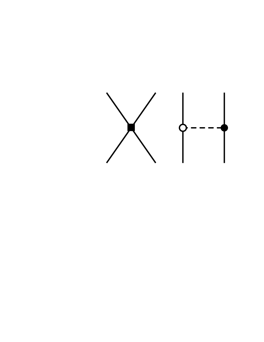
Figure 1: Feynman diagrams contributing to the $\bar{N}N$ interaction at leading order in the covariant power counting. The solid lines denote nucleons/antinucleons, and the dashed line represents the pion. The box denotes the vertex from $\mathcal{L}_{\bar{N}N}^{(0)}$, while the circle/dot shows vertex from $\mathcal{L}_{\pi\bar{N}}^{(1)}$/$\mathcal{L}_{\pi N}^{(1)}$.

The $\bar{N}N$ interaction contains scattering and annihilation potentials, which reads

$$V_{\bar{N}N}=V^{\text{S}}+V^{\text{A}}.$$ (1)

For the scattering process, the underlying covariant power counting of the $\bar{N}N$ interaction is the same as the $NN$ case, which is described in detail in Refs. Ren et al. (2018); Xiao et al. (2019); Lu et al. (2022), because the antinucleon field (spinor $v$) and the nucleon field (spinor $u$) are treated on an equal footing as spin-1/2 fields. The corresponding Feynman diagrams at LO are summarized in Fig. 1, and the relevant Lagrangians are,

$$\mathcal{L}_{\text{eff.}}=\mathcal{L}_{\pi\pi}^{(2)}+\mathcal{L}_{\pi\bar{N}}^{(1)}+\mathcal{L}_{\pi N}^{(1)}+\mathcal{L}_{\bar{N}N}^{(0)},$$ (2)

where the superscript denotes the chiral dimension. The lowest order $\pi\pi$, $\pi\bar{N}$, $\pi N$, and $\bar{N}N$ Lagrangians read,

$$\mathcal{L}_{\pi\pi}^{(2)}= \frac{f_{\pi}^{2}}{4}\text{Tr}\left[\partial_{\mu}U\partial^{\mu}U^{\dagger}+\left(U+U^{\dagger}\right)m_{\pi}^{2}\right],$$ (3)

$$\mathcal{L}_{\pi\bar{N}}^{(1)}= \mathcal{L}_{\pi N}^{(1)}=\bar{\Psi}\left(i\not{D}-M+\frac{g_{A}}{2}\gamma^{\mu}\gamma_{5}u_{\mu}\right)\Psi,$$ (4)

$$\mathcal{L}_{\bar{N}N}^{(0)}= C_{S}\left(\bar{\Psi}\Psi\right)\left(\bar{\Psi}\Psi\right)+C_{A}\left(\bar{\Psi}\gamma_{5}\Psi\right)\left(\bar{\Psi}\gamma_{5}\Psi\right)$$ (5)

$$+ C_{V}\left(\bar{\Psi}\gamma_{\mu}\Psi\right)\left(\bar{\Psi}\gamma^{\mu}\Psi\right)$$

$$+ C_{AV}\left(\bar{\Psi}\gamma_{\mu}\gamma_{5}\Psi\right)\left(\bar{\Psi}\gamma^{\mu}\gamma_{5}\Psi\right)$$

$$+ C_{T}\left(\bar{\Psi}\sigma_{\mu\nu}\Psi\right)\left(\bar{\Psi}\sigma^{\mu\nu}\Psi\right),$$

with the pion decay constant $f_{\pi}=92.4$ MeV, the axial coupling constant $g_{A}=1.29$ Machleidt and Entem (2011), the $SU(2)$ matrix $U=u^{2}=\text{exp}\left(\frac{i\Phi}{f_{\pi}}\right)$, where $\Phi$ and $\Psi$ are,

$$\Phi=\left(\begin{matrix}\pi^{0}&\sqrt{2}\pi^{+}\\ \sqrt{2}\pi^{-}&-\pi^{0}\end{matrix}\right),~{}~{}~{}~{}\Psi=\left(\begin{matrix}p\\ n\end{matrix}\right).$$ (6)

The covariant derivative of the nucleon field $\Psi$ is defined as,

$$D_{\mu}\Psi =\partial_{\mu}\psi+\left[\Gamma_{\mu},\Psi\right],$$ (7)

$$\Gamma_{\mu} =\frac{1}{2}\left(u^{\dagger}\partial_{\mu}u+u\partial_{\mu}u^{\dagger}\right),$$ (8)

and the axial current $u_{\mu}$ is,

$$u_{\mu}=i\left(u^{\dagger}\partial_{\mu}u-u\partial_{\mu}u^{\dagger}\right).$$ (9)

The covariant scattering potentials at leading order $V^{\text{S}}_{\text{LO}}$ can be obtained by summing the contact (CT) and one-pion-exchange (OPE) terms shown in Fig. 1,

$$V_{\text{LO}}^{\text{S}}=V^{\text{S}}_{\text{CT}}+V^{\text{S}}_{\text{OPE}},$$ (10)

where the contact potential $V^{\text{S}}_{\text{CT}}$ is,

$$V^{\text{S}}_{\text{CT}}\left(\bm{p},\bm{p}^{\prime}\right)= C_{S}\left[\bar{v}\left(\bm{p},s_{1}\right)v\left(\bm{p}^{\prime},s_{1}^{\prime}\right)\right]\left[\bar{u}\left(-\bm{p}^{\prime},s_{2}^{\prime}\right)u\left(-\bm{p},s_{2}\right)\right]+C_{A}\left[\bar{v}\left(\bm{p},s_{1}\right)\gamma_{5}v\left(\bm{p}^{\prime},s_{1}^{\prime}\right)\right]\left[\bar{u}\left(-\bm{p}^{\prime},s_{2}^{\prime}\right)\gamma_{5}u\left(-\bm{p},s_{2}\right)\right]$$ (11)

$$+ C_{V}\left[\bar{v}\left(\bm{p},s_{1}\right)\gamma_{\mu}v\left(\bm{p}^{\prime},s_{1}^{\prime}\right)\right]\left[\bar{u}\left(-\bm{p}^{\prime},s_{2}^{\prime}\right)\gamma^{\mu}u\left(-\bm{p},s_{2}\right)\right]+C_{AV}\left[\bar{v}\left(\bm{p},s_{1}\right)\gamma_{\mu}\gamma_{5}v\left(\bm{p}^{\prime},s_{1}^{\prime}\right)\right]\left[\bar{u}\left(-\bm{p}^{\prime},s_{2}^{\prime}\right)\gamma^{5}\gamma_{5}u\left(-\bm{p},s_{2}\right)\right]$$

$$+ C_{T}\left[\bar{v}\left(\bm{p},s_{1}\right)\sigma_{\mu\nu}v\left(\bm{p}^{\prime},s_{1}^{\prime}\right)\right]\left[\bar{u}\left(-\bm{p}^{\prime},s_{2}^{\prime}\right)\sigma^{\mu\nu}u\left(-\bm{p},s_{2}\right)\right],$$

and the one-pion-exchange potential $V^{\text{S}}_{\text{OPE}}$ is

$$V^{\text{S}}_{\text{OPE}}\left(\bm{p},\bm{p}^{\prime}\right)=\frac{g_{A}^{2}}{4f_{\pi}^{2}}\frac{\left[\bar{v}\left(\bm{p},s_{1}\right)\bm{\tau}_{1}\gamma_{\mu}\gamma_{5}q^{\mu}v\left(\bm{p}^{\prime},s_{1}^{\prime}\right)\right]\left[\bar{u}\left(-\bm{p}^{\prime},s_{2}^{\prime}\right)\bm{\tau}_{2}\gamma_{\nu}\gamma_{5}q^{\nu}u\left(-\bm{p},s_{2}\right)\right]}{\left(E_{p^{\prime}}-E_{p}\right)^{2}-\left(\bm{p}^{\prime}-\bm{p}\right)^{2}-m_{\pi}^{2}},$$ (12)

where $p$/$p^{\prime}$ is the incoming/outgoing three momentum, $m_{\pi}$ refers to the pion mass and we use the isospin-averaged value $m_{\pi}=138$ MeV, $q^{\mu}=\left(E_{p^{\prime}}-E_{p},\bm{p}^{\prime}-\bm{p}\right)$, and $\bm{\tau}$ is the isospin Pauli matrix. The Dirac spinor $u(\bm{p},s)$ is,

$$u(\bm{p},s)=N_{p}\left(\begin{matrix}1\\ \frac{\bm{\sigma}\cdot\bm{p}}{\epsilon_{p}}\end{matrix}\right)\chi_{s},~{}~{}~{}~{}N_{p}=\sqrt{\frac{\epsilon_{p}}{2m_{N}}},$$ (13)

where $m_{N}$ refers to the nucleon mass, and we use the isospin-averaged value $m_{N}=939$ MeV, $\epsilon_{p}=E_{p}+m_{N}$, $\chi_{s}$ denotes the Pauli spinor matrix, and $\bm{\sigma}$ is the Pauli matrix. The Spinor $v\left(\bm{p},s\right)=\gamma_{0}Cu^{*}\left(\bm{p},s\right)$ with $C$ represents the charge transformation operator,

$$C=i\gamma_{0}\gamma_{2}=\left(\begin{matrix}0&i\bm{\sigma}_{2}\\ i\bm{\sigma}_{2}&0\end{matrix}\right).$$ (14)

The antinucleon-nucleon contact terms include one antinucleon field $v$, one nucleon field $u$, and their adjoint fields $\bar{v}$ and $\bar{u}$. The different arrangements of these four-baryon fields are of the following schematic form:

$$\sum_{i}C_{i}\left[\bar{v}\left(\bm{p},s_{1}\right)\Gamma_{i}v\left(\bm{p}^{\prime},s_{1}^{\prime}\right)\right]\left[\bar{u}\left(-\bm{p}^{\prime},s_{2}^{\prime}\right)\Gamma^{i}u\left(-\bm{p},s_{2}\right)\right],$$

$$\sum_{i}C_{i}\left[\bar{v}\left(\bm{p},s_{1}\right)\Gamma_{i}u\left(-\bm{p},s_{2}\right)\right]\left[\bar{u}\left(-\bm{p}^{\prime},s_{2}^{\prime}\right)\Gamma^{i}v\left(\bm{p}^{\prime},s_{1}^{\prime}\right)\right],$$

$$\sum_{i}C_{i}\left[\bar{v}\left(\bm{p},s_{1}\right)\Gamma_{i}u\left(-\bm{p},s_{2}\right)\right]\left[\bar{u}\left(\bm{p}^{\prime},s_{1}^{\prime}\right)\Gamma^{i}v\left(-\bm{p}^{\prime},s_{2}^{\prime}\right)\right],$$

$$\sum_{i}C_{i}\left[\bar{v}\left(\bm{p},s_{1}\right)\Gamma_{i}v\left(-\bm{p}^{\prime},s_{2}^{\prime}\right)\right]\left[\bar{u}\left(\bm{p}^{\prime},s_{1}^{\prime}\right)\Gamma^{i}u\left(-\bm{p},s_{2}\right)\right],$$

where $C_{i\in\{S,A,V,AV,T\}}$ refers to the low-energy constants and $\Gamma_{i}$ is the corresponding Clifford algebra. Using the generalized Fierz identities Nieves and Pal (2004), a product of two bilinears can be rearranged as

$$\bm{e}\left(1234\right)=\bm{K}^{\left(abcd\right)}\bm{e}\left(abcd\right),$$ (15)

where $\bm{e}\left(abcd\right)$ represents an ordering of quadrilinears and $\bm{K}^{\left(abcd\right)}$ is the transformation matrix, whose explicit forms are given in the Appendix A. This allows one to express all the arrangements as a linear combination of the chosen type, in our case, Eq. (11). Here the $C_{A}\left[\bar{v}\left(\bm{p},s_{1}\right)\gamma_{5}v\left(\bm{p}^{\prime},s_{1}^{\prime}\right)\right]\left[\bar{u}\left(-\bm{p}^{\prime},s_{2}^{\prime}\right)\gamma_{5}u\left(-\bm{p},s_{2}\right)\right]$ term, which arises from the next-to-leading order potential according to Refs. Xiao et al. (2019); Lu et al. (2022), is ascended to leading order to ensure that one can make use of the generalized Fierz identities to get rid of redundant terms in the potential.

In computing the observables, it is convenient to transform the potentials into the $LSJ$ basis, where $L$ denotes the total orbital angular momentum, $S$ is the total spin, and $J$ is the total angular momentum. The procedure for the partial wave projection is standard Erkelenz et al. (1971); Erkelenz (1974). The explicit expression for the OPE potential in the $LSJ$ basis is of the opposite sign as that in the $NN$ case given in Ref. Ren et al. (2018) after partial wave projection, while the contact potentials are of the following form,

$$V^{\text{S}}_{1S0}=\xi\left[C_{1S0}\left(R_{p}^{2}+R_{p^{\prime}}^{2}\right)+\hat{C}_{1S0}\left(1+R_{p}^{2}R_{p^{\prime}}^{2}\right)\right],$$

$$V^{\text{S}}_{3P0}=\xi C_{3P0}R_{p}R_{p^{\prime}},$$

$$V^{\text{S}}_{1P1}=2\xi\left(C_{3S1}-3\hat{C}_{3S1}\right)R_{p}R_{p^{\prime}},$$

$$V^{\text{S}}_{3P1}=\frac{4}{3}\xi\left(C_{1S0}-\hat{C}_{1S0}\right)R_{p}R_{p^{\prime}},$$

$$V^{\text{S}}_{3S1}=\xi\left[C_{3S1}\left(R_{p}^{2}+R_{p^{\prime}}^{2}\right)+\hat{C}_{3S1}\left(9+R_{p}^{2}R_{p^{\prime}}^{2}\right)\right],$$

$$V^{\text{S}}_{3D1}=8\xi\hat{C}_{3S1}R_{p}^{2}R_{p^{\prime}}^{2},$$

$$V^{\text{S}}_{3S1-3D1}=2\sqrt{2}\xi\left(2C_{3S1}R_{p}^{2}+\hat{C}_{3S1}R_{p}^{2}R_{p^{\prime}}^{2}\right),$$

$$V^{\text{S}}_{3D1-3S1}=2\sqrt{2}\xi\left(2C_{3S1}R_{p^{\prime}}^{2}+\hat{C}_{3S1}R_{p}^{2}R_{p^{\prime}}^{2}\right),$$ (16)

where $\xi=-4\pi N_{p}^{2}N_{p^{\prime}}^{2}$, $R_{p}=|\bm{p}|/\epsilon_{p}$, and $R_{p^{\prime}}=|\bm{p^{\prime}}|/\epsilon_{p^{\prime}}$. The low-energy constants are linear combinations of $C_{S,A,V,AV,T}$ of the following form,

$$C_{1S0}=C_{A}+C_{AV}-6C_{T}+3C_{V},$$

$$\hat{C}_{1S0}=3C_{AV}+C_{S}-6C_{T}+C_{V},$$

$$C_{3P0}=-2\left(C_{A}-4C_{AV}+C_{S}-12C_{T}-4C_{V}\right),$$

$$C_{3S1}=\frac{1}{3}\left(-C_{A}-C_{AV}-2C_{T}+C_{V}\right),$$

$$\hat{C}_{3S1}=\frac{1}{9}\left(-C_{AV}+C_{S}+2C_{T}+C_{V}\right).$$ (17)

The covariant contact potential contributes to all $J=0,1$ partial waves with 5 independent rearranged low-energy constants $C_{1S0},\hat{C}_{1S0},C_{3S1},\hat{C}_{3S1}$, and $C_{3P0}$. The ${}^{1}P_{1},^{3}P_{1},^{3}D_{1},^{3}S_{1}-^{3}D_{1}$, and ${}^{3}D_{1}-^{3}S_{1}$ potentials are constrained only by the $S$-wave parameters, which allow us to check the relativistic corrections to the short-range $\bar{N}N$ interaction. The Pauli principle does not hold in the $\bar{N}N$ interaction, so the number of low-energy constants is twice that of the $NN$ case.

Compared to the $NN$ interaction, a new feature of the $\bar{N}N$ interaction is the presence of the annihilation process, which leads to an intrinsic difficulty in describing a system that has hundreds of annihilation many-body channels at rest Carbonell et al. (2023). Here, we follow the approach of Ref. Kang et al. (2014) that manifestly fulfills unitarity and considers the annihilation potential of the following form,

$$V^{\text{A}}=\sum_{X=2\pi,3\pi,...}V_{\bar{N}N\rightarrow X}G_{X}V_{X\rightarrow\bar{N}N},$$ (18)

where $X$ is the sum over all open annihilation channels, and $G_{X}$ is the propagator of the intermediate state $X$. Making use of the identity

$$\frac{1}{x\pm i\epsilon}=\mathcal{P}\frac{1}{x}\mp i\pi\delta\left(x\right),$$ (19)

The imaginary part of Eq. (18) is constrained by,

$$\text{Im}V^{\text{A}}=-\pi\sum_{X}V_{\bar{N}N\rightarrow X}V_{X\rightarrow\bar{N}N}.$$ (20)

Then, expanding $V_{\bar{N}N\rightarrow X}$ in powers of the nucleon three momentum up to next-to-leading order (NLO), one can obtain the annihilation potential,

$$V_{1S0}^{\text{A}}=-i\left(C_{1S0}^{a}+\hat{C}_{1S0}^{a}\frac{p^{2}}{4m_{N}^{2}}\right)\left(C_{1S0}^{a}+\hat{C}_{1S0}^{a}\frac{p^{\prime 2}}{4m_{N}^{2}}\right),$$

$$V_{3P0}^{\text{A}}=-i\left(C_{3P0}^{a}\right)^{2}\frac{pp^{\prime}}{4m_{N}^{2}},$$

$$V_{1P1}^{\text{A}}=-i\left(C_{1P1}^{a}\right)^{2}\frac{pp^{\prime}}{4m_{N}^{2}},$$

$$V_{3P1}^{\text{A}}=-i\left(C_{3P1}^{a}\right)^{2}\frac{pp^{\prime}}{4m_{N}^{2}},$$

$$V_{3S1}^{\text{A}}=-i\left(C_{3S1}^{a}+\hat{C}_{3S1}^{a}\frac{p^{2}}{4m_{N}^{2}}\right)\left(C_{3S1}^{a}+\hat{C}_{3S1}^{a}\frac{p^{\prime 2}}{4m_{N}^{2}}\right),$$

$$V_{3S1-3D1}^{\text{A}}=-i\left(C_{3S1}^{a}+\hat{C}_{3S1}^{a}\frac{p^{2}}{4m_{N}^{2}}\right)C_{\epsilon_{1}}^{a}\frac{p^{\prime 2}}{4m_{N}^{2}},$$

$$V_{3D1-3S1}^{\text{A}}=-iC_{\epsilon_{1}}^{a}\frac{p^{2}}{4m_{N}^{2}}\left(C_{3S1}^{a}+\hat{C}_{3S1}^{a}\frac{p^{\prime 2}}{4m_{N}^{2}}\right),$$

$$V_{3D1}^{\text{A}}=-i\left(C_{\epsilon_{1}}^{a}\right)^{2}\frac{p^{2}p^{\prime 2}}{16m_{N}^{4}}.$$ (21)

The factors $\frac{1}{4m_{N}^{2}}$ and $\frac{1}{16m_{N}^{4}}$ are introduced to ensure that all annihilation constants are of the same dimension. There are several issues to address regarding the annihilation potential. 1) Eq. (II) only contains the $J=0,1$ partial waves to be consistent with the scattering potential given in Eq. (II). 2) Eq. (II) is organized in the conventional Weinberg power counting, while a more self-consistent annihilation potential should be constructed in the covariant power counting. The main difficulty in evaluating a covariant annihilation potential is the complexity of the explicit expressions for all open annihilation potentials $V_{\bar{N}N\rightarrow X}$. Based on the experience in the $NN$ interaction, the accuracy of the covariant potential is comparable to the non-relativistic potential at one order higher. Therefore, we expand $V_{\bar{N}N\rightarrow X}$ up to NLO in the conventional Weinberg power counting to evaluate the annihilation potential as an approximation of the exact covariant annihilation potential at LO. 3) The full annihilation potential contains a real part from the principal value in Eq. (18), whose structure is accounted for by the LECs in the conventional non-relativistic scattering potential at the corresponding order. By contrast, the contribution of the real part of Eq. (18) can only be absorbed in the covariant LECs partly in our case because the number of independent LECs in the covariant power counting at LO is less than that in the non-relativistic power counting at NLO. However, this real part does not break unitarity. In addition, the contribution to the $\bar{N}N$ interaction from the additional structures is suppressed because it is of order $\mathcal{O}\left(p^{2}\right)$ (here $p$ refers to the small quantity in the conventional Weinberg power counting). Therefore, we use the pure imaginary potential in Eq. (II) to account for the annihilation process in practice. It should be mentioned that the problem above can be solved by constructing a self-consistent annihilation potential in the covariant power counting. We will explore how to implement this idea in the future.

III Scattering equation and phase shifts

The partial wave projected scattering $T$-matrix is obtained by solving the Kadyshevsky equation in the $LSJ$ basis,

$$T^{SJ}_{L^{\prime},L}\left(p^{\prime},p\right) =V^{SJ}_{L^{\prime},L}\left(p^{\prime},p\right)+\sum_{L^{\prime\prime}}\int_{0}^{+\infty}\frac{k^{2}\text{d}k}{\left(2\pi\right)^{3}}V^{SJ}_{L^{\prime},L}\left(p^{\prime},k\right)$$

$$\times\frac{m_{N}^{2}}{2\left(k^{2}+m_{N}^{2}\right)}\frac{1}{\sqrt{p^{2}+m_{N}^{2}}-\sqrt{k^{2}+m_{N}^{2}}+i\epsilon}$$

$$\times T^{SJ}_{L^{\prime\prime},L}\left(k,p\right).$$ (22)

We separately solve the Kadyshevsky in the isospin basis for $I=0$ and $I=1$ and fit the resulting phase shifts to those in Ref. Zhou and Timmermans (2012) to determine the corresponding LECs. To remove the ultraviolet divergences, the potential is regularized with a non-local Gaussian-type cut-off function,

$$f^{\Lambda}\left(p,p^{\prime}\right)=\exp\left[-\left(p^{6}+p^{\prime 6}\right)/\Lambda^{6}\right],$$ (23)

with the cut-off value varied in the range $\Lambda=450-600$ MeV. We use the non-local cut-off function so that the contribution of the contact term in each partial wave is not mixed.

The partial wave $S$ matrix is related to the on-shell $T$ matrix by,

$$S^{SJ}_{L^{\prime},L}\left(p\right)=\delta_{L^{\prime},L}-i\frac{p~{}m_{N}^{2}}{8\pi^{2}E_{p}}T^{SJ}_{L^{\prime},L}\left(p\right).$$ (24)

Phase shifts and mixing angles can be obtained from the matrix $S$ using the idea of “Stapp” Stapp et al. (1957). The annihilation process makes the phase shifts complex for the $\bar{N}N$ interaction. We follow the procedure of Ref. Bystricky, J. et al. (1987) to evaluate the phase shifts. For uncoupled channels, the real and imaginary parts of the phase shift $\delta_{L}$ can be obtained from the on-shell $S$ matrix,

$$\text{Re}\left(\delta_{L}\right) =\frac{1}{2}\arctan\frac{\text{Im}\left(S_{L}\right)}{\text{Re}\left(S_{L}\right)},$$

$$\text{Im}\left(\delta_{L}\right) =-\frac{1}{2}\log\lvert S_{L}\rvert.$$ (25)

For coupled channels, the phase shifts $\delta_{L\pm 1}$ and mixing angles $\epsilon_{J}$ are,

$$\text{Re}\left(\delta_{L\pm 1}\right) =\frac{1}{2}\arctan\frac{\text{Im}\left(\eta_{L\pm 1}\right)}{\text{Re}\left(\eta_{L\pm 1}\right)},$$

$$\text{Im}\left(\delta_{L\pm 1}\right) =-\frac{1}{2}\log\lvert\eta_{L\pm 1}\rvert,$$

$$\epsilon_{J} =\frac{1}{2}\arctan\left(\frac{i\left(S_{L-1,L-1}+S_{L+1,L+1}\right)}{2\sqrt{S_{L-1,L-1}S_{L+1,L+1}}}\right),$$

where $\eta_{L}=\frac{S_{L,L}}{\cos 2\epsilon_{J}}$.

IV Results and discussions

In the fitting procedure, we perform a simultaneous fit to the $J=0,1$ PWA of Ref. Zhou and Timmermans (2012) at laboratory energies below 125 MeV $\left(p_{\text{lab}}\leq 500~{}\text{MeV}\right)$ with cutoff values varying in the range $\Lambda=450-600$ MeV, except for the ${}^{1}S_{0}$ and ${}^{3}P_{0}$ partial waves with $I=1$, where we consider extra data at $p_{\text{lab}}=600$ MeV because of the resonance-like behaviors. Table 1 lists the numerical values of the LECs. The values for $\hat{C}_{3S1}$ are of one or two orders of magnitude smaller than $C_{3S1}$. Still, its contribution to the ${}^{3}S_{1}$ potential is comparable to that from $C_{3S1}$ because the contribution to the ${}^{3}S_{1}$ potential from $C_{3S1}$ is suppressed by $1/\left(4m_{N}^{2}\right)$ to some extent since it is multiplied by $R_{p}^{2},R_{p^{\prime}}^{2}$. A similar situation occurs in the ${{}^{1}S_{0}}$ partial wave and the annihilation process.

Table 1: LO low-energy constants for different cutoffs. The parameters related to the scattering process are in units of $10^{4}$ GeV^-2, while the parameters related to the annihilation process are in units of $10^{2}$ GeV^-1

LEC		$\Lambda=450$ MeV	$\Lambda=600$ MeV
$I=0$	$C_{1S0}$	$0.213$	$0.154$
	$\hat{C}_{1S0}$	$0.031$	$0.013$
	$C_{1S0}^{a}$	$-1.080$	$0.668$
	$\hat{C}_{1S0}^{a}$	$20.987$	$-9.199$
	$C_{3P0}$	$-0.019$	$-0.117$
	$C_{3P0}^{a}$	$1.472$	$0.971$
	$C_{1P1}^{a}$	$1.281$	$1.478$
	$C_{3P1}^{a}$	$0.737$	$0.447$
	$C_{3S1}$	$-0.043$	$-0.025$
	$\hat{C}_{3S1}$	$0.001$	$0.0002$
	$C_{3S1}^{a}$	$0.207$	$-0.388$
	$\hat{C}_{3S1}^{a}$	$4.533$	$3.326$
	$C_{\epsilon 1}^{a}$	$-1.982$	$0.743$
$I=1$	$C_{1S0}$	$-0.051$	$0.016$
	$\hat{C}_{1S0}$	$-0.004$	$0.025$
	$C_{1S0}^{a}$	$-0.398$	$1.270$
	$\hat{C}_{1S0}^{a}$	$4.730$	$-14.110$
	$C_{3P0}$	$0.242$	$0.179$
	$C_{3P0}^{a}$	$1.177$	$0.570$
	$C_{1P1}^{a}$	$1.270$	$1.066$
	$C_{3P1}^{a}$	$1.336$	$1.214$
	$C_{3S1}$	$0.014$	$0.032$
	$\hat{C}_{3S1}$	$0.001$	$0.001$
	$C_{3S1}^{a}$	$0.211$	$-0.081$
	$\hat{C}_{3S1}^{a}$	$9.208$	$-4.512$
	$C_{\epsilon 1}^{a}$	$1.720$	$-2.078$

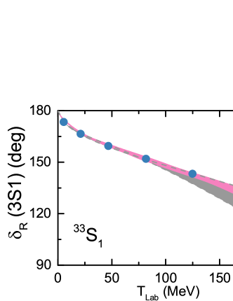
(a)

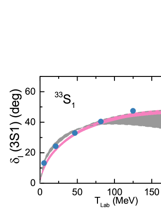
(b)

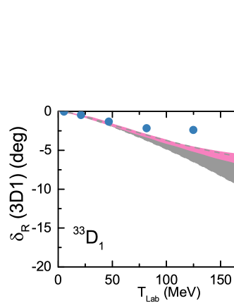
(c)

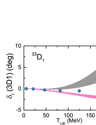
(d)

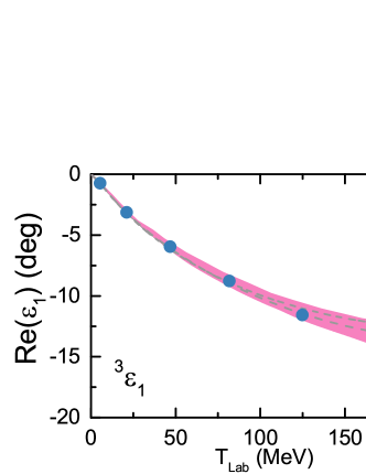
(e)

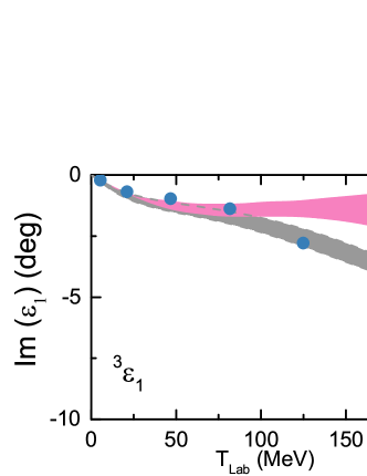
(f)

Figure 5: Same as Fig. 2, but for the ${{}^{3}S_{1}}-{{}^{3}D_{1}}$ partial waves with $I=1$.

The phase shifts obtained in our study, the NLO non-relativistic results Kang et al. (2014), and the $\bar{N}N$ PWA Zhou and Timmermans (2012) for laboratory energies up to $200$ MeV are shown in Figs. 2-5. The partial waves are labeled in the spectral notation ${}^{\left(2I+1\right)\left(2S+1\right)}L_{J}$, and the bands are generated by varying the cutoff in the range $\Lambda=450-600$ MeV for both the relativistic and non-relativistic calculations. The LO non-relativistic phase shifts are not included for comparison because the annihilation potential, in this case, is only non-zero for the ${}^{1}S_{0}$ and ${}^{3}S_{1}$ partial waves. Hence, the descriptions of the phase shifts of other partial waves are very bad. In addition, even for the ${}^{1}S_{0}$ and ${}^{3}S_{1}$ partial waves, the differences between the LO non-relativistic phase shifts and the PWA are significant compared with the differences between the NLO non-relativistic phase shifts and the PWA.

The LO relativistic results of the $J=0$ partial waves agree with the PWA for the energy region shown here. Compared with its NLO non-relativistic counterpart, the overall cutoff dependence of the LO relativistic phase shifts is weaker, especially for the real parts of the phase shifts of the $I=1$ partial waves. At the same time, one can observe a sizeable cutoff dependence in the NLO non-relativistic results for energies above $150$ MeV because of the resonance-like behaviors. Since the number of free parameters for the $J=0$ partial waves in the LO relativistic and NLO non-relativistic potentials is identical ($4$ for the ${}^{1}S_{0}$ partial wave and $2$ for the ${}^{3}P_{0}$ partial wave, including annihilation parameters), the relatively weaker cutoff dependence has to do with the relativistic corrections of the scattering equation and the scattering potentials at orders higher than $\mathcal{O}\left(p^{2}\right)$ (in the conventional Weinberg power counting). Note that the NLO non-relativistic results are obtained by fitting to the PWA of Ref. Zhou and Timmermans (2012) at $p_{\text{lab}}\leq 500$ MeV, while in our study one more datum at $p_{\text{lab}}=600$ MeV is also included in the fitting process for the ${}^{31}S_{0}$ and ${}^{33}P_{0}$ partial waves as explained above. However, adapting the same fitting strategy in the NLO non-relativistic framework ruins the descriptions of PWA at $p_{\text{lab}}\leq 500$ MeV. Therefore, the improvement in the cutoff dependence in the relativistic framework cannot be completely attributed to the differences in the fitting procedures. An exception exists in the imaginary part of the phase shift of the ${}^{11}S_{0}$ partial wave, where the cutoff dependence of the LO relativistic results is sizeable at laboratory energies above $150$ MeV. This is related to the description of the ${}^{13}P_{1}$ partial wave, whose PWA yields a negative phase at low energies, which tends to become positive at higher energies. As argued in Ref. Kang et al. (2014), reproducing such phase shifts requires a repulsive potential at large separations of the antinucleon and nucleon but becomes attractive at short distances. Since the scattering potential for ${}^{3}P_{1}$ is controlled by the LECs in the ${}^{1}S_{0}$ partial wave as shown in Eq. II, the description of $\delta_{\text{I}}\left({}^{11}S_{0}\right)$ is influenced by the demand for such an attractive potential. Improvement might be possible at NLO.

For the $J=1$ uncoupled channels, the LO relativistic and NLO non-relativistic results are comparable. The NLO non-relativistic result is better for the imaginary part of the phase shift in the ${}^{11}P_{1}$ partial wave. In comparison, the LO relativistic results are better for the real part of the phase shift in the ${}^{31}P_{1}$ partial wave. Still, the relativistic corrections are not attractive enough to account for the discrepancies between the calculated phase shifts and the PWA. As for other partial waves, both results are comparable, but the cutoff dependence of the LO relativistic results is weaker than that of the NLO non-relativistic results at laboratory energies above 150 MeV, in analogy to the results for the ${}^{31}S_{0}$ and ${}^{33}P_{0}$ partial waves. It should be emphasized that the LO relativistic scattering potentials for the ${}^{1}P_{1}$ and ${}^{3}P_{1}$ partial waves are determined by $S$- wave LECs as shown in Eq. (II). In contrast, the NLO non-relativistic scattering potentials contain as many LECs as the annihilation potentials. Thus, the improvements in the cutoff dependence must originate from the relativistic corrections.

For the $J=1$ coupled channels, the $S$-wave phase shifts are generally well reproduced. The ${}^{3}D_{1}$ phase shift and mixing angle $\epsilon_{1}$ show strong cutoff dependence. However, it is not so surprising since they have no free parameters. The intriguing thing is that the relativistic corrections shift the trends of $\delta_{\text{I}}\left({}^{33}D_{1}\right)$ and $\text{Im}\left(\epsilon_{1}\right)$ to the right direction at laboratory energies above $100$ MeV compared to their non-relativistic counterparts. However, the correction seems too large for the ${}^{33}D_{1}$ partial wave. As a result, the cutoff dependence of $\delta_{\text{I}}\left({}^{33}S_{1}\right)$ becomes large at that energy region.

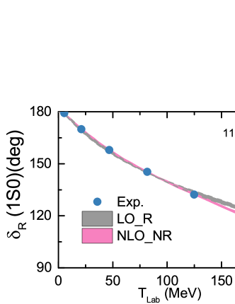
(a)

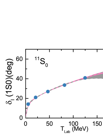
(b)

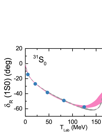
(c)

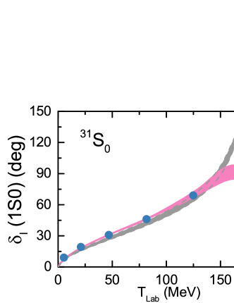
(d)

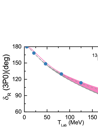
(e)

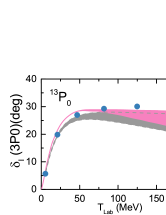
(f)

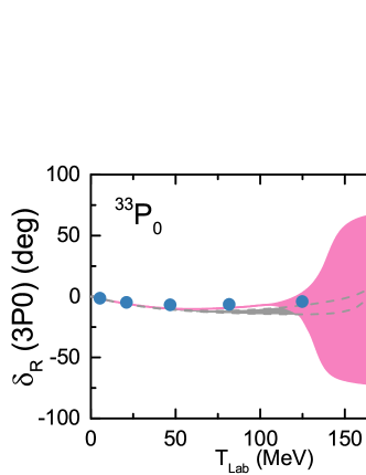
(g)

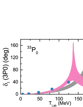
(h)

Figure 2: Real and imaginary parts of the phase shift for the ${}^{1}S_{0}$ and ${}^{3}P_{0}$ partial waves. The gray bands show the LO relativistic chiral EFT results with the cutoff in the range $\Lambda$ = 450–600 MeV. The pink bands show the NLO non-relativistic chiral EFT results of Ref. Kang et al. (2014). The blue dots refer to the solution of the PWA of Ref. Zhou and Timmermans (2012).

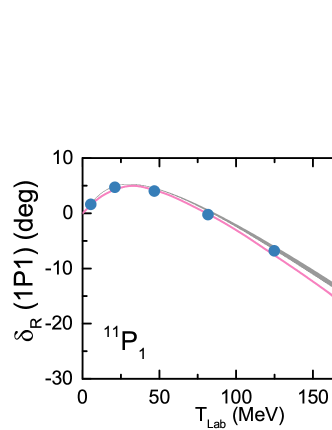
(a)

(b)

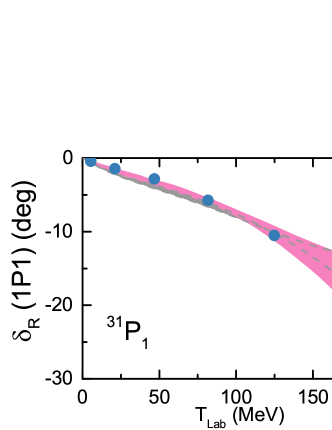
(c)

(d)

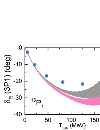
(e)

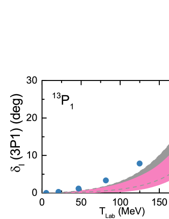
(f)

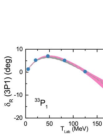
(g)

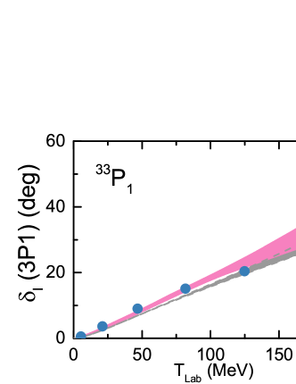
(h)

Figure 3: Same as Fig. 2, but for the ${}^{1}P_{1}$ and ${}^{3}P_{1}$ partial waves.

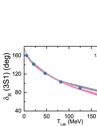
(a)

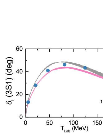
(b)

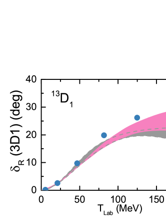
(c)

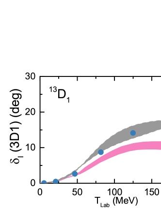
(d)

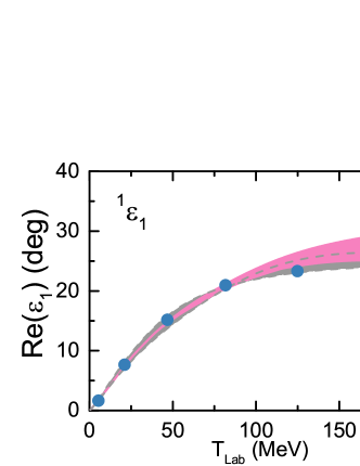
(e)

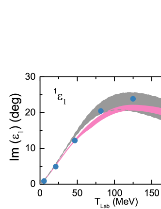
(f)

Figure 4: Same as Fig. 2, but for the ${{}^{3}S_{1}}-{{}^{3}D_{1}}$ partial waves with $I=0$.

Next, we turn to the near-threshold $\bar{N}N$ structures. The phase shifts shown in Figs. 2- 5 suggest the existence of bound states in the ${}^{11}S_{0},^{13}P_{0},^{13}S_{1},$ and ${}^{33}S_{1}$ channels because their phase shifts are about $180^{\circ}$ at threshold. Therefore, we search for possible bound states at the energy region near the $\bar{N}N$ threshold. The corresponding binding energies obtained with our relativistic potential and the NLO non-relativistic potential Kang et al. (2014) are summarized in Table 2. Although these structures have complex $E_{B}$, and the sign of the real part of $E_{B}$ is even positive in some cases, according to Refs. Kang et al. (2014); Badalian et al. (1982), the poles that we found can still be referred to as bound states because they lie on the physical sheet and move below the threshold when the annihilation potential is switched off. Note that compared to the NLO non-relativistic results, a bound state emerges in the ${}^{33}S_{1}$ channel with a relatively large width, which reflects the differences in the potentials of the ${}^{33}S_{1}-^{33}D_{1}$ coupled channel. Moreover, We also find a deeply bound state with $E_{B}=\left(-102.2,-152.5\right)-\text{i}\left(79.1,199.3\right)$ MeV in the ${}^{11}S_{0}$ channel, whose quantum number is consistent with the pseudoscalar interpretation of $X(1835)$, $X(1840)$, and $X(1880)$ suggested by the BESIII Collaboration Ablikim et al. (2005, 2024), despite that it is located far below the $\bar{N}N$ threshold and our result suffer relatively large uncertainties. A firm conclusion can only be drawn once reliable theoretical uncertainties can be estimated. We want to mention that the studies employing the semi-phenomenological $\bar{N}N$ interactions have found a bound state in the ${}^{11}S_{0}$ channel Yan et al. (2005); Sibirtsev et al. (2005); Ding and Yan (2005); Dedonder et al. (2009), although the predicted binding energies are rather different. Therefore, a NLO study is needed to confirm the nature of this state. Apart from the bound states, the phase shifts exhibit resonance-like structures in ${}^{31}S_{0}$ and ${}^{33}P_{0}$ partial waves at energies above $150$ MeV. Thus, we also look for poles in the second Riemann sheet in these two channels. However, we do not find any resonant states in this energy region.

Table 2: $\bar{N}N$ bound states and their binding energies. The uncertainties originate from the variation of the cutoff in the range $\Lambda=450-600$ MeV.

Partial Wave	$E_{B}$ (MeV)
	LO relativistic	NLO non-relativistic Kang et al. (2014)
${}^{11}S_{0}$	$\left(-102.2,-152.5\right)-\text{i}\left(79.1,199.3\right)$	No near-threshold structure
${}^{13}P_{0}$	$\left(-1.5,-2.1\right)-\text{i}\left(20.2,21.0\right)$	$\left(-1.1,1.9\right)-\text{i}\left(17.8,22.4\right)$
${}^{13}S_{1}$	$\left(-7.1,28.8\right)-\text{i}\left(45.5,49.2\right)$	$\left(5.6,7.7\right)-\text{i}\left(49.2,60.5\right)$
${}^{33}S_{1}$	$\left(-17.6,7.0\right)-\text{i}\left(128.9,134.4\right)$	No near-threshold structure

V Summary and Outlook

We have studied the $\bar{N}N$ interaction in the covariant chiral effective field theory. The $\bar{N}N$ potential was calculated at LO, and the corresponding LECs were determined by fitting to the phase shifts and inelasticities provided by the PWA of the $\bar{p}p$ scattering data Zhou and Timmermans (2012). The overall description of the PWA with the LO relativistic potential is comparable to that obtained with the NLO non-relativistic potential, similar to the situation observed in the $NN$ interaction. In addition, we searched for near $\bar{N}N$ threshold structures, and found several bound states in the ${}^{11}S_{0},^{13}P_{0},^{13}S_{1}$, and ${}^{33}S_{1}$ channels. The quantum number of ${}^{11}S_{0}$ supports the pseudoscalar interpretation of $X(1835)$, $X(1840)$, and $X(1880)$ observed by the BESIII Collaboration. However, the mass of this bound state is much smaller than $X(1835)$, $X(1840)$, and $X(1880)$. A NLO study is needed to confirm the nature of this state. We note that there is a bound state with a binding energy $E_{B}=\left(-17.6,7.0\right)-\text{i}\left(128.9,134.4\right)\text{MeV}$ in the ${}^{33}S_{1}$ channel, which is, however, missing in the non-relativistic interaction.

Although the $\bar{p}p$ data can be described reasonably well in the relativistic approach, comparable to or even slightly better than the NLO non-relativistic results, further refinements can still be made. For example, the annihilation potential is approximated in the conventional Weinberg power counting, the theoretical uncertainties are estimated roughly by varying the cutoff, and full renormalization group invariance has not been achieved. We will study these issues in the future.

VI Acknowledgments

This work was supported in part by the National Key R&D Program of China under Grant No.2023YFA1606700, the National Natural Science Foundation of China under Grants No.12347113, and the Chinese Postdoctoral Science Foundation under Grants No.2022M720360. We thank Dr. Xian-Wei Kang for the enlightening discussions regarding the annihilation potential. Yang Xiao thanks Dr. Chun-Xuan Wang for the valuable discussions.

Appendix A Generalized Fierz identities

This section briefly introduces the generalized Fierz identities; a detailed derivation can be found in Ref. Nieves and Pal (2004). We start with some notations. The Clifford algebra $\Gamma_{i}$ matrices are,

$$\Gamma_{S} =\mathbbm{1},$$

$$\Gamma_{V} =\gamma_{\mu},$$

$$\Gamma_{T} =\sigma^{\mu\nu},$$

$$\Gamma_{AV} =i\gamma^{\mu}\gamma_{5},$$

$$\Gamma_{A} =\gamma_{5}.$$ (26)

An ordering of quadrilinears is defined as

$$e_{I}\left(1234\right)=\left(\bar{\Psi}_{1}\Gamma_{I}\Psi_{2}\right)\left(\bar{\Psi}_{3}\Gamma^{I}\Psi_{4}\right),$$ (27)

where $I\in\{S,A,V,AV,T\}$. In this notation, the standard Fierz transformation gives the relation between the $e_{I}(1234)$ and the $e_{J}(1432)$,

$$e_{I}\left(1234\right)=\sum_{J}F_{IJ}e_{J}\left(1432\right),$$ (28)

where $F_{IJ}$ is the matrix element of a $4\times 4$ matrix $\bm{F}$,

$$\bm{F}=\frac{1}{4}\left(\begin{matrix}1&1&\frac{1}{2}&-1&1\\ 4&-2&0&-2&-4\\ 12&0&-2&0&12\\ -4&-2&0&-2&4\\ 1&-1&\frac{1}{2}&1&1\end{matrix}\right).$$ (29)

Eq. (27) can be abbreviated as

$$\bm{e}\left(1234\right)=\bm{F}\left(1432\right).$$ (30)

In the standard Fierz relation, the exchanged spinors remain the same type, i.e., a $u$-spinor/$v$-spinor remains a $u$-spinor/$v$-spinor. It is possible to interchange a pair of $u$-spinors to $v$-spinors in quadrilinears. For illustration, we consider a simple example where we want to interchange the positions of the spinors in the first and second place. The results of other rearrangements can be obtained similarly. Consider a quadrilinear

$$e_{I}\left(2^{c}1^{c}34\right)=\left(\bar{\Psi}^{c}\Gamma_{I}\Psi^{c}\right)\left(\bar{\Psi}\Gamma^{I}\Psi\right),$$ (31)

where $\Psi^{c}$ denotes that if $\Psi$ is a $u$-spinor, $\Psi^{c}$ is a $v$-spinor and vice versa. $\Psi^{c}$ and $\Psi$ are related by,

$${\Psi}^{c}=\gamma_{0}C{\Psi}^{*},$$ (32)

with $C$ the aforementioned charge transformation operator, and

$$C^{-1}\Gamma_{I}C=\eta_{I}\Gamma_{I}^{\mathrm{T}},$$ (33)

with the value of $\eta_{I}$ is

$$\eta_{I}=\left\{\begin{matrix}+1&I=S,AV,A\\ -1&I=V,T\end{matrix}\right..$$ (34)

Using Eq. (33) and some matrix algebra, we obtain

$$\bar{\Psi}\Gamma_{I}\Psi=-\eta_{I}\bar{\Psi}^{c}\Gamma_{I}\Psi^{c}.$$ (35)

Therefore, we obtain the relation between the quadrilinears $e_{I}\left(1234\right)$ and the quadrilinears that the position of the first and second spinors are interchanged $e_{J}\left(2^{c}1^{c}34\right)$,

$$e_{I}\left(1234\right)=\sum_{J}S_{IJ}e_{J}\left(2^{c}1^{c}34\right),$$ (36)

where $S_{IJ}$ is the element of the matrix

$$\bm{S}=\text{diag}\left(-1,+1,+1,-1,-1\right).$$ (37)

Following the procedure introduced above and making full use of the standard Fierz transformations, we can obtain the generalized Fierz identities,

$$\bm{e}\left(1234\right)=\bm{K}^{(abcd)}\bm{e}(abcd),$$ (38)

where the matrix $K$ is summarized in Table 3.

Table 3: Fierz matrices for all scalar combinations.

Final order	$\bm{K}$
$(1234)$	$\mathbbm{1}$
$(1432)$	$\bm{F}$
$(2^{c}1^{c}34)$	$\bm{S}$
$(124^{c}3^{c})$	$\bm{S}$
$(13^{c}2^{c}4)$	$\bm{SFS}$
$(13^{c}4^{c}2)$	$\bm{SF}$
$(142^{c}3^{c})$	$\bm{FS}$
$(2^{c}1^{c}4^{c}3^{c})$	$\bm{SS}=\mathbbm{1}$
$(31^{c}2^{c}4)$	$\bm{SF}$
$(31^{c}4^{c}2)$	$\bm{SFS}$
$(4^{c}1^{c}2^{c}3^{c})$	$\bm{F}$
$(4^{c}1^{c}32)$	$\bm{FS}$

References

- Bai et al. (2003) J. Z. Bai et al. (BES), Phys. Rev. Lett. 91, 022001 (2003), arXiv:hep-ex/0303006 .
- Ablikim et al. (2005) M. Ablikim et al. (BES), Phys. Rev. Lett. 95, 262001 (2005), arXiv:hep-ex/0508025 .
- Ablikim et al. (2012) M. Ablikim et al. (BESIII), Phys. Rev. Lett. 108, 112003 (2012), arXiv:1112.0942 [hep-ex] .
- Ablikim et al. (2016) M. Ablikim et al. (BESIII), Phys. Rev. Lett. 117, 042002 (2016), arXiv:1603.09653 [hep-ex] .
- Ablikim et al. (2022) M. Ablikim et al. (BESIII), Phys. Rev. Lett. 129, 022002 (2022), arXiv:2112.14369 [hep-ex] .
- Ablikim et al. (2024) M. Ablikim et al. (BESIII), Phys. Rev. Lett. 132, 151901 (2024), arXiv:2310.17937 [hep-ex] .
- Abe et al. (2002a) K. Abe et al. (Belle), Phys. Rev. Lett. 88, 181803 (2002a), arXiv:hep-ex/0202017 .
- Abe et al. (2002b) K. Abe et al. (Belle), Phys. Rev. Lett. 89, 151802 (2002b), arXiv:hep-ex/0205083 .
- Aubert et al. (2005) B. Aubert et al. (BaBar), Phys. Rev. D 72, 051101 (2005), arXiv:hep-ex/0507012 .
- Aubert et al. (2006) B. Aubert et al. (BaBar), Phys. Rev. D 73, 012005 (2006), arXiv:hep-ex/0512023 .
- Yuan and Karliner (2021) C.-Z. Yuan and M. Karliner, Phys. Rev. Lett. 127, 012003 (2021), arXiv:2103.06658 [hep-ex] .
- Sturm et al. (2010) C. Sturm, B. Sharkov, and H. Stöcker, Nucl. Phys. A 834, 682c (2010).
- Peng et al. (2020) H. P. Peng, Y. H. Zheng, and X. R. Zhou, Physics 49, 513 (2020).
- Dover and Richard (1980) C. B. Dover and J. M. Richard, Phys. Rev. C 21, 1466 (1980).
- Dover and Richard (1982) C. B. Dover and J. M. Richard, Phys. Rev. C 25, 1952 (1982).
- Cote et al. (1982) J. Cote, M. Lacombe, B. Loiseau, B. Moussallam, and R. Vinh Mau, Phys. Rev. Lett. 48, 1319 (1982).
- Timmers et al. (1984) P. H. Timmers, W. A. van der Sanden, and J. J. de Swart, Phys. Rev. D 29, 1928 (1984), [Erratum: Phys.Rev.D 30, 1995 (1984)].
- Hippchen et al. (1991) T. Hippchen, J. Haidenbauer, K. Holinde, and V. Mull, Phys. Rev. C 44, 1323 (1991).
- Mull et al. (1991) V. Mull, J. Haidenbauer, T. Hippchen, and K. Holinde, Phys. Rev. C 44, 1337 (1991).
- Mull and Holinde (1995) V. Mull and K. Holinde, Phys. Rev. C 51, 2360 (1995), arXiv:nucl-th/9411014 .
- Entem and Fernandez (2006) D. R. Entem and F. Fernandez, Phys. Rev. C 73, 045214 (2006).
- El-Bennich et al. (2009) B. El-Bennich, M. Lacombe, B. Loiseau, and S. Wycech, Phys. Rev. C 79, 054001 (2009), arXiv:0807.4454 [nucl-th] .
- Weinberg (1990) S. Weinberg, Phys. Lett. B 251, 288 (1990).
- Weinberg (1991) S. Weinberg, Nucl. Phys. B 363, 3 (1991).
- Weinberg (1992) S. Weinberg, Phys. Lett. B 295, 114 (1992), arXiv:hep-ph/9209257 .
- Ordonez et al. (1994) C. Ordonez, L. Ray, and U. van Kolck, Phys. Rev. Lett. 72, 1982 (1994).
- van Kolck (1994) U. van Kolck, Phys. Rev. C 49, 2932 (1994).
- Epelbaum et al. (2015) E. Epelbaum, H. Krebs, and U. G. Meißner, Phys. Rev. Lett. 115, 122301 (2015), arXiv:1412.4623 [nucl-th] .
- Reinert et al. (2018) P. Reinert, H. Krebs, and E. Epelbaum, Eur. Phys. J. A 54, 86 (2018), arXiv:1711.08821 [nucl-th] .
- Entem et al. (2017) D. R. Entem, R. Machleidt, and Y. Nosyk, Phys. Rev. C 96, 024004 (2017), arXiv:1703.05454 [nucl-th] .
- Machleidt (2023) R. Machleidt, Few Body Syst. 64, 77 (2023), arXiv:2307.06416 [nucl-th] .
- Chen and Ma (2011) G. Y. Chen and J. P. Ma, Phys. Rev. D 83, 094029 (2011), arXiv:1101.4071 [hep-ph] .
- Kang et al. (2014) X.-W. Kang, J. Haidenbauer, and U.-G. Meißner, JHEP 02, 113 (2014), arXiv:1311.1658 [hep-ph] .
- Dai et al. (2017) L.-Y. Dai, J. Haidenbauer, and U.-G. Meißner, JHEP 07, 078 (2017), arXiv:1702.02065 [nucl-th] .
- Haidenbauer et al. (2014) J. Haidenbauer, X. W. Kang, and U. G. Meißner, Nucl. Phys. A 929, 102 (2014), arXiv:1405.1628 [nucl-th] .
- Yang et al. (2023a) Q.-H. Yang, D. Guo, L.-Y. Dai, J. Haidenbauer, X.-W. Kang, and U.-G. Meißner, Sci. Bull. 68, 2729 (2023a), arXiv:2206.01494 [nucl-th] .
- Cheng and Kang (2018) H.-Y. Cheng and X.-W. Kang, Phys. Lett. B 780, 100 (2018), arXiv:1712.00566 [hep-ph] .
- Dai et al. (2018) L.-Y. Dai, J. Haidenbauer, and U.-G. Meißner, Phys. Rev. D 98, 014005 (2018), arXiv:1804.07077 [hep-ph] .
- Yang et al. (2023b) Q.-H. Yang, D. Guo, and L.-Y. Dai, Phys. Rev. D 107, 034030 (2023b), arXiv:2209.10101 [hep-ph] .
- Haidenbauer and Meißner (2020) J. Haidenbauer and U.-G. Meißner, Chin. Phys. C 44, 033101 (2020), arXiv:1910.14423 [hep-ph] .
- Epelbaum et al. (2018) E. Epelbaum, A. M. Gasparyan, J. Gegelia, and U.-G. Meißner, Eur. Phys. J. A 54, 186 (2018), arXiv:1810.02646 [nucl-th] .
- van Kolck (2020) U. van Kolck, Front. in Phys. 8, 79 (2020), arXiv:2003.06721 [nucl-th] .
- Zhou et al. (2022) D. Zhou, B. Long, R. G. E. Timmermans, and U. van Kolck, Phys. Rev. C 105, 054005 (2022), arXiv:2203.06840 [nucl-th] .
- Geng et al. (2008) L. S. Geng, J. Martin Camalich, L. Alvarez-Ruso, and M. J. Vicente Vacas, Phys. Rev. Lett. 101, 222002 (2008), arXiv:0805.1419 [hep-ph] .
- Lensky and Pascalutsa (2010) V. Lensky and V. Pascalutsa, Eur. Phys. J. C 65, 195 (2010), arXiv:0907.0451 [hep-ph] .
- Alarcon et al. (2012) J. M. Alarcon, J. Martin Camalich, and J. A. Oller, Phys. Rev. D 85, 051503 (2012), arXiv:1110.3797 [hep-ph] .
- Martin Camalich et al. (2010) J. Martin Camalich, L. S. Geng, and M. J. Vicente Vacas, Phys. Rev. D 82, 074504 (2010), arXiv:1003.1929 [hep-lat] .
- Ren et al. (2012) X. L. Ren, L. S. Geng, J. Martin Camalich, J. Meng, and H. Toki, JHEP 12, 073 (2012), arXiv:1209.3641 [nucl-th] .
- Lu et al. (2023) J.-X. Lu, L.-S. Geng, M. Doering, and M. Mai, Phys. Rev. Lett. 130, 071902 (2023), arXiv:2209.02471 [hep-ph] .
- Ren et al. (2018) X.-L. Ren, K.-W. Li, L.-S. Geng, B.-W. Long, P. Ring, and J. Meng, Chin. Phys. C 42, 014103 (2018), arXiv:1611.08475 [nucl-th] .
- Xiao et al. (2019) Y. Xiao, L.-S. Geng, and X.-L. Ren, Phys. Rev. C 99, 024004 (2019), arXiv:1812.03005 [nucl-th] .
- Lu et al. (2022) J.-X. Lu, C.-X. Wang, Y. Xiao, L.-S. Geng, J. Meng, and P. Ring, Phys. Rev. Lett. 128, 142002 (2022), arXiv:2111.07766 [nucl-th] .
- Ren et al. (2021) X.-L. Ren, C.-X. Wang, K.-W. Li, L.-S. Geng, and J. Meng, Chin. Phys. Lett. 38, 062101 (2021), arXiv:1712.10083 [nucl-th] .
- Wang et al. (2021) C.-X. Wang, L.-S. Geng, and B. Long, Chin. Phys. C 45, 054101 (2021), arXiv:2001.08483 [nucl-th] .
- Xiao et al. (2020) Y. Xiao, C.-X. Wang, J.-X. Lu, and L.-S. Geng, Phys. Rev. C 102, 054001 (2020), arXiv:2007.13675 [nucl-th] .
- Wang et al. (2022) C.-X. Wang, J.-X. Lu, Y. Xiao, and L.-S. Geng, Phys. Rev. C 105, 014003 (2022), arXiv:2110.05278 [nucl-th] .
- Bai et al. (2020) Q.-Q. Bai, C.-X. Wang, Y. Xiao, and L.-S. Geng, Phys. Lett. B, 135745 (2020), arXiv:2007.01638 [nucl-th] .
- Bai et al. (2022) Q.-Q. Bai, C.-X. Wang, Y. Xiao, J.-X. Lu, and L.-S. Geng, Phys. Lett. B 833, 137347 (2022), arXiv:2105.06113 [hep-ph] .
- Girlanda et al. (2019) L. Girlanda, A. Kievsky, M. Viviani, and L. E. Marcucci, Phys. Rev. C 99, 054003 (2019), arXiv:1811.09398 [nucl-th] .
- Zou et al. (2024) W.-J. Zou, J.-X. Lu, P.-W. Zhao, L.-S. Geng, and J. Meng, Phys. Lett. B 854, 138732 (2024), arXiv:2312.15672 [nucl-th] .
- Zhou and Timmermans (2012) D. Zhou and R. G. E. Timmermans, Phys. Rev. C 86, 044003 (2012), arXiv:1210.7074 [hep-ph] .
- Machleidt and Entem (2011) R. Machleidt and D. R. Entem, Phys. Rept. 503, 1 (2011), arXiv:1105.2919 [nucl-th] .
- Nieves and Pal (2004) J. F. Nieves and P. B. Pal, Am. J. Phys. 72, 1100 (2004), arXiv:hep-ph/0306087 .
- Erkelenz et al. (1971) K. Erkelenz, R. Alzetta, and K. Holinde, Nucl. Phys. A 176, 413 (1971).
- Erkelenz (1974) K. Erkelenz, Phys. Rept. 13, 191 (1974).
- Carbonell et al. (2023) J. Carbonell, G. Hupin, and S. Wycech, Eur. Phys. J. A 59, 259 (2023), arXiv:2309.14831 [nucl-th] .
- Stapp et al. (1957) H. P. Stapp, T. J. Ypsilantis, and N. Metropolis, Phys. Rev. 105, 302 (1957).
- Bystricky, J. et al. (1987) Bystricky, J., Lechanoine-Leluc, C., and Lehar, F., J. Phys. France 48, 199 (1987).
- Badalian et al. (1982) A. M. Badalian, L. P. Kok, M. I. Polikarpov, and Y. A. Simonov, Phys. Rept. 82, 31 (1982).
- Yan et al. (2005) M.-L. Yan, S. Li, B. Wu, and B.-Q. Ma, Phys. Rev. D 72, 034027 (2005), arXiv:hep-ph/0405087 .
- Sibirtsev et al. (2005) A. Sibirtsev, J. Haidenbauer, S. Krewald, U.-G. Meissner, and A. W. Thomas, Phys. Rev. D 71, 054010 (2005), arXiv:hep-ph/0411386 .
- Ding and Yan (2005) G.-J. Ding and M.-L. Yan, Phys. Rev. C 72, 015208 (2005), arXiv:hep-ph/0502127 .
- Dedonder et al. (2009) J. P. Dedonder, B. Loiseau, B. El-Bennich, and S. Wycech, Phys. Rev. C 80, 045207 (2009), arXiv:0904.2163 [nucl-th] .