Global Rewards in Restless Multi-Armed Bandits
Abstract
Restless multi-armed bandits (rmab) extend multi-armed bandits so pulling an arm impacts future states. Despite the success of rmabs, a key limiting assumption is the separability of rewards into a sum across arms. We address this deficiency by proposing restless-multi-armed bandit with global rewards (rmab-g), a generalization of rmabs to global non-separable rewards. To solve rmab-g, we develop the Linear- and Shapley-Whittle indices, which extend Whittle indices from rmabs to rmab-gs. We prove approximation bounds but also point out how these indices could fail when reward functions are highly non-linear. To overcome this, we propose two sets of adaptive policies: the first computes indices iteratively, and the second combines indices with Monte-Carlo Tree Search (MCTS). Empirically, we demonstrate that our proposed policies outperform baselines and index-based policies with synthetic data and real-world data from food rescue.
1 Introduction
Restless multi-armed bandits (rmab) are models of resource allocation that combine multi-armed bandits with states for each bandit’s arm. Such a model is “restless” because arms can change state even when not pulled. rmabs are an enticing framework because optimal decisions can be efficiently made using pre-computed Whittle indices [1, 2]. As a result, rmab have been used in scheduling [3], autonomous driving [4], multichannel access [5], and maternal health [6].
The existing rmab model assumes that rewards are separable into a sum of per-arm rewards. However, many real-world objectives are non-separable functions of the arms pulled. We find this situation in food rescue platforms. These platforms notify subsets of volunteers about upcoming food rescue trips and aim to maximize the trip completion rate [7]. When modeling this with rmabs, arms correspond to volunteers, arm pulls correspond to notifications, and the reward corresponds to the trip completion rate. The trip completion rate is non-separable as we only need one volunteer to complete each trip (more details in Section 3). Beyond food rescue, rmabs can potentially model problems in peer review [8], blood donation [9], and emergency dispatch [10], but the rewards are again non-separable.
Motivated by these situations, we propose the restless multi-armed bandit with global rewards (rmab-g), a generalization of rmabs to non-separable rewards. Whittle indices from rmabs [1] fail for rmab-gs due to the non-separability of the reward. Because of this, we propose a generalization of Whittle indices to global rewards called the Linear-Whittle and Shapley-Whittle indices. Our approximation bounds demonstrate that these policies perform well for near-linear rewards but struggle for highly non-linear rewards. We address this by developing adaptive policies that combine Linear- and Shapley-Whittle indices with search techniques. We empirically verify that adaptive policies outperform index-based and baseline approaches on synthetic and food rescue datasets. 111We plan to release code and all non-proprietary data after the camera ready
Our contributions are: (1) We propose the rmab-g problem, which extends rmabs to situations with global rewards. We additionally characterize the difficulty of solving and approximating rmab-gs; (2) We develop the Linear-Whittle and Shapley-Whittle indices, which extend Whittle indices for global rewards, and detail approximation bounds; (3) We design a set of adaptive policies which combine Linear- and Shapley-Whittle indices with greedy and Monte Carlo Tree Search (MCTS) algorithms; and (4) We empirically demonstrate that adaptive policies improve upon baselines and pre-computed index-based policies for the rmab-g problem with synthetic and food rescue datasets.
2 Background and Notation
An instance of restless multi-armed bandits (rmabs) consists of arms, each of which is defined through the following Markov Decision Process (mdp): . Here, is the state space, is the action space, is a reward function, is a transition function detailing the probability of an arm transitioning into a new state, and is a discount factor. For a time period , we define the state of all arm as , and for each round, a planner takes action ; we drop the superscript when clear from context. Following prior work [11, 6], we assume throughout this paper to represent not pulling and pulling an arm respectively. A planner chooses subject to a budget , so that at most arms can be pulled in each time step: . The objective is to find a policy, that maximizes the discounted total reward, summed over all arms:
| (1) |
To solve an rmab, one can pre-compute the “Whittle index” for each arm and possible state : , where , and . Here, represents the expected future reward for playing action , given a penalty for pulling an arm. The Whittle index computes the minimum penalty needed to prevent arm pulls; larger penalties () indicate more value for pulling an arm. In each round, the planner pulls the arms with the largest Whittle indices given the states of the arms. Such a Whittle index-based policy is asymptotically optimal [1, 2].
3 Defining Restless Multi-Armed Bandits with Global Rewards
Objectives in rmabs are written as the sum of per-arm rewards (Equation 1), while real-world objectives involve non-separable rewards. For example, food rescue organizations, which notify volunteers about food rescue trips, aim to maximize the trip completion rate, i.e., the fraction of completed trips. Suppose we model volunteers as arms and volunteer notifications as arm pulls. Then arm states correspond to volunteer engagement (e.g., active or inactive) and rewards are the probability that any notified volunteers complete the rescue. Here, we cannot split the reward into per-volunteer functions.
Inspired by situations such as food rescue, we propose the restless multi-armed bandit with global rewards (rmab-g) problem, which generalizes rmabs to problems with a global reward function:
Definition 1.
We define an instance of rmab-g through the following MDP for each arm: . The aim is to find a policy, , that maximizes:
| (2) |
Throughout this paper, we focus on scenarios where is monotonic and submodular in ; , where is submodular and monotonic. Such rewards have diminishing returns as extra arms are pulled. We select this because a) monotonic and submodular functions can be efficiently optimized [12] and b) submodular functions are ubiquitous [13, 14, 8].
Our problem formulation can model various real-world scenarios including notification decisions in food rescue and reviewer assignments in peer review [8]. In food rescue, let be the probability that a volunteer picks up a given trip, given their state, . The global reward is the probability that any notified volunteer accepts a trip: . In peer review, journals select reviewers for submissions where selection impacts future reviewer availability [8]. The goal is to select a subset of available reviewers with comprehensive subject-matter expertise. If reviewer expertise is a set , then we maximize the overlap between the required expertise, , and the expertise across selected () and available () reviewers: . Our formulation inherits the per-arm reward from rmabs as there may be per-arm rewards. For example, food rescue platforms might care about the number of active volunteers, so .
Let . We characterize the difficulty of rmab-g:
Theorem 1.
The restless multi-armed bandit with global rewards is PSPACE-Hard.
Theorem 2.
No polynomial time algorithm can achieve better than a approximation to the restless multi-armed bandit with global rewards problem.
Theorem 3.
Consider an rmab-g instance . Let and let be the optimal policy. Let . Suppose , , monotonic and submodular in and , and submodular in . Then, with oracle access to we can compute in time so .
Theorem 1 and 2 demonstrate the difficulty of finding solutions to rmab-gs while Theorem 3 describes a potential panacea via . Leveraging is the best polynomial-time algorithm (due to matching bounds from Theorem 2 and 3), but the exponential state space makes it difficult to learn such a , motivating the need for better algorithms (we empirically demonstrate this in Section 6.1). We prove Theorem 1 through reduction from rmab, Theorem 2 through reduction from submodular optimization, and Theorem 3 through induction on value iteration. Full proofs are in Appendix K.
4 Linear-Whittle and Shapley-Whittle Indices
4.1 Defining Linear-Whittle and Shapley-Whittle
Because the Whittle index policy is optimal for rmabs [2], we investigate its extension to rmab-gs. We develop two extensions: the Linear-Whittle policy, which computes marginal rewards for each arm, and the Shapley-Whittle policy, which computes Shapley values for each arm. To define the Linear-Whittle policy, we define the marginal reward as , where is a vector with 1 at index and elsewhere. The Linear-Whittle policy linearizes the global reward by optimistically estimating and computing the Whittle index from this:
Definition 2.
Linear-Whittle - Consider an instance of rmab-g . Define , where . Then the Linear-Whittle index is . The Linear-Whittle policy pulls arms with the highest Linear-Whittle indices.
To improve on the Linear-Whittle policy, we develop the Shapley-Whittle policy, which uses Shapley values to linearize the global reward. The Linear-Whittle policy linearizes global rewards via , but this approximation could be loose as . The Shapley value, , improves this by averaging marginal rewards across subsets of arms (see Shapley et al. [15]). Let be the element-wise maximum, so means arms in and arm are pulled. Define:
| (3) |
Here, captures the added value of pulling arm , when are already pulled. While the Linear-Whittle policy estimates the global reward as , the Shapley-Whittle policy estimates the global reward as . The Linear-Whittle policy overestimates marginal contributions, as (proof in Appendix L), so by using Shapley values, we take a pessimistic approach (by taking the minimum over all ). This approach could lead to more accurate estimates of :
Definition 3.
Shapley-Whittle - Consider an instance of rmab-g . Let , where . Then the Shapley-Whittle index is . The Shapley-Whittle policy pulls arms with the highest Shapley-Whittle indices.
4.2 Approximation Bounds
To characterize the performance of our policies, we prove approximation bounds:
Theorem 4.
For any fixed set of transitions, , let for some . For an rmab-g , let , and let the induced linear rmab be . Let be the Linear-Whittle policy, and let . Define as
| (4) |
If the induced linear rmab is irreducible and indexable with the uniform global attractor property, then asymptotically in for any set of transitions, .
Theorem 5.
For any fixed set of transitions, , let for some . For an rmab-g , let , and let the induced Shapley rmab be . Let be the Shapley-Whittle policy, and let . Define as
| (5) |
If the induced Shapley rmab is irreducible and indexable with the uniform global attractor property, then asymptotically in for any choice of transitions, .
Corollary 5.1.
Let be the Linear-Whittle policy, and for some . Then for any .
lower bounds policy performance; small does not guarantee poor performance but large guarantees good performance. For example, and are near for near-linear global rewards, so Linear- and Shapley-Whittle policies perform well in those situations. We prove all three Theorems by bounding the gap between the linear (or Shapley) approximation and (proofs in Appendix L). We note that the assumptions made by all Theorems are the same assumptions needed for the optimality of Whittle indices [2]. We present an example of these lower bounds:
Example 4.1.
Consider an scenario for rmab-g with . Let and . Here, are sets corresponding to each arm, with , and . Let for all , and consider the Linear-Whittle policy. Next, note that , so .
Now let and let . Here, , while . Therefore, , so the Linear-Whittle policy is a approximation to this problem.
We describe upper bounds and apply these bounds to Example 4.1.
Theorem 6.
Let . For a set of transitions , let and . Define as follows:
| (6) |
Then there exists some transitions, , and initial state , so that
Theorem 7.
Let . For a set of transitions and initial state , let and . Let be:
| (7) |
Then there exists some transitions, and initial state so that
Example 4.2.
Recall the situation from Example 4.1. Let for all , and consider the Linear-Whittle policy. Construct construct , so that or in other words, . The Linear-Whittle policy will pull arms and , as . This results in an action , so that , while the optimal action is with . Computing matches this upper bound of in this scenario.
Our upper bounds demonstrate that, for any reward function, there exists a set of transitions where our policies perform a -fraction worse than optimal. is small when the optimal action diverges from the action taken by the Linear-Whittle policy (analogously for Shapley-Whittle). Such situations occur because policies fail to account for inter-arm interactions (e.g. Example 4.2). We present lower bounds using the average reward because Whittle optimality holds in that situation. Otherwise, we follow prior work, and focus on discounted reward [11] (for more discussion see Ghosh et al. [16])
5 Adaptive Approaches for RMAB-G
5.1 Limitations of Pre-Computed Index-Based Policies
Despite the approximation bounds given in Appendix L, Linear- and Shapley-Whittle policies can exhibit poor performance when upper bounds and are small. We detail such a situation:
Lemma 8.
(Informal) Let be either the Linear or Shapley-Whittle policies. There exist problem settings where will achieve an approximation ratio no better than .
In general, pre-computed index-based policies perform poorly because of their inability to consider inter-arm interactions (proof in Appendix L). This approximation ratio matches lower bounds, , which motivates new policies which select arms adaptively.
5.2 Iterative Whittle Indices
Lemma 8 motivates the need for policies that select arms adaptively and go beyond pre-computed indices. Based on this, we propose two new policies: Iterative Linear-Whittle and Iterative Shapley-Whittle. Both policies compute current time step rewards, , based on the arms pulled, .
Definition 4.
Iterative Linear-Whittle - Consider an instance of rmab-g . Consider a state , and construct a new state, , with . Let and for . Then the Iterative Linear-Whittle index is , where
Definition 5.
Iterative Shapley-Whittle - Consider an instance of rmab-g , with defined by Equation 3. Construct a new state, , with . Let and for . Then the Iterative Shapley-Whittle Index is . Here is computed as:
| (8) |
By incorporating the arms pulled, , both policies better estimate the present reward. Here, represents the expected discounted reward when receiving currently and in the future (similarly for Shapley-Whittle). To model this, we construct a new state, , which mirrors except for the reward in the current timestep. The Iterative Linear-Whittle and Shapley-Whittle policies then iteratively select arms that maximize and respectively and stop after selecting arms.
5.3 MCTS-based Approaches
To improve upon the greedy selection done by iterative policies, we combine Monte Carlo Tree Search (mcts) with Whittle indices. mcts allows us to look beyond greedy selection by searching through various arm combinations. We propose two policies: MCTS Linear-Whittle and MCTS Shapley-Whittle. For both, we search through arm combinations, , compute the present value (), and estimate the future value via Linear- and Shapley-Whittle indices. Nodes in the mcts tree correspond to arm combinations, edges to individual arms, and leaf nodes to actions .
Our implementation of mcts matches the upper confidence tree algorithm for selection, expansion, and backpropogation [17], while we differ for rollout (details in Appendix C). During rollout, we select nodes according to an -greedy algorithm [18] and leverage the Linear- and Shapley-Whittle policies for greedy selection. We do so because -greedy is a simple strategy that could potentially improve upon random rollouts. Once at a leaf node, the reward is for MCTS Linear-Whittle and for MCTS Shapley-Whittle. Here, is the known current value, and is the estimated future value when accounting for the present reward .
6 Experiments
We evaluate our policies across both synthetic and real-world datasets. We compare our six policies (Section 4.1, Section 5.2, and Section 5.3) to the following baselines (more details in Appendix B):
-
1.
Random - We uniform randomly select arms at each timestep.
-
2.
Vanilla Whittle - We run the vanilla Whittle index, which optimizes only for .
-
3.
Greedy - We select actions which have the highest value of .
-
4.
MCTS - We run mcts up to some depth, , where is a constant.
- 5.
-
6.
DQN Greedy - Inspired by Theorem 3, we first learn a dqn then greedily optimize .
-
7.
Optimal - We compute the optimal policy through value iteration when .
We run all experiments for 15 seeds and 5 trials per seed. We report the normalized reward, which is the accumulated discounted reward divided by that of the random policy. This normalization is due to differences in magnitudes within and across problem instances and we use discounted rewards due to prior work [11]. We additionally compute the standard error across all runs.
6.1 Results with Synthetic Data
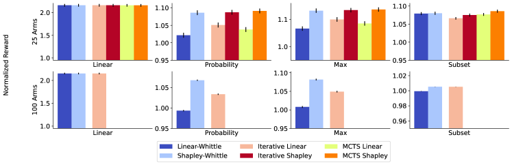
To understand performance across synthetic scenarios, we develop synthetic problem instances that leverage each of the following global reward functions (details on and choices in Appendix A):
-
1.
Linear - Given , then .
-
2.
Probability - Given , then .
-
3.
Max - Given , then .
-
4.
Subset - Given sets, , , then .
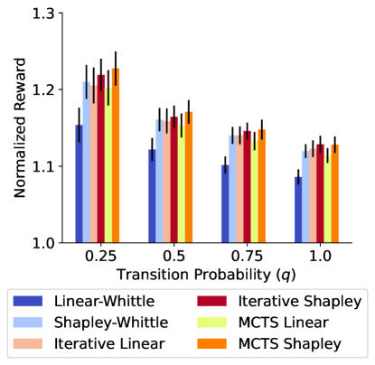
We select these rewards, as they range from linear or near-linear (Linear and Probability) to highly non-linear (Max and Subset). The reward functions can also be employed to model real-world situations; the Probability reward models food rescue and the Subset reward models peer review (see Section 3). For all rewards, we let and , which matches prior work [6]. We construct synthetic transitions parameterized by , so , where is the uniform distribution (see Appendix A). We construct transition probabilities so that having or only improves transition probabilities (see Wang et al. [11]). We vary in Appendix G and find that our choice of does not impact findings. Unless otherwise specified, we fix .
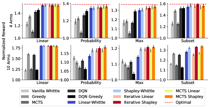
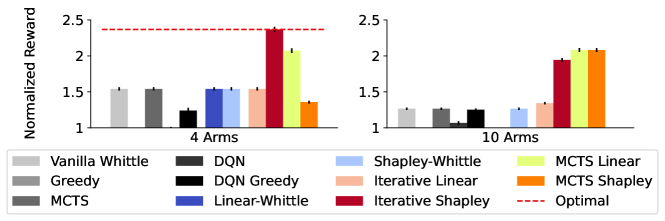
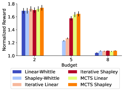
Figure 1 shows that our policies consistently outperform baselines. Among our policies, Iterative and MCTS Shapley-Whittle policies perform best. For , Iterative and MCTS Shapley-Whittle significantly outperform baselines (paired t-test ) and index-based policies except for the Linear reward (). dqn-based policies regress from on average worse for to on average worse for compared to our best policy, which occurs due to the exponential state space. In Appendix I, we consider more combinations of and and find similar results.
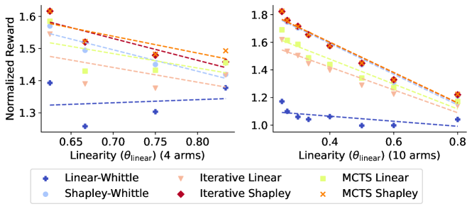
To understand policy performance across rewards, we analyze how reward linearity impacts performance. We quantify linearity via (see Theorem 6) and compute for Subset instances varying in (see Appendix A). For non-linear reward functions (small ), Iterative and MCTS-Shapley-Whittle are best, outperforming Linear-Whittle by 56%, while for near-linear reward functions (large ), all policies are within 18% of each other (Figure 2, ). Appendix H shows that, for some rewards, adaptive policies outperform non-adaptive policies by 50%.
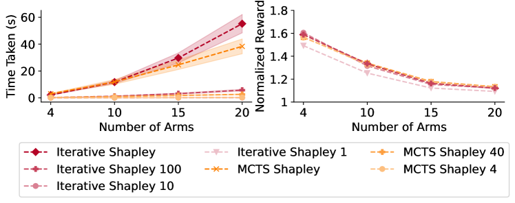
To understand the tradeoff between efficiency and performance we plot the time taken and normalized reward for various (Figure 3). We evaluate variants of Iterative Shapley-Whittle and MCTS Shapley-Whittle because both perform well yet are computationally expensive. For Iterative Shapley-Whittle, 1000 samples are used for Shapley estimation by default, so we consider variants that use 100, 10, and 1 samples. For MCTS Shapley-Whittle, we run 400 iterations of MCTS by default, so we consider variants that run 40 and 4 iterations. Iterative Shapley-Whittle policies are the slowest but can be made faster without impacting performance by reducing the number of samples. Our results demonstrate how we can develop efficient adaptive policies which perform well.
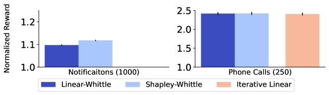
6.2 Results with Real-World Data in Food Rescue
To evaluate our policies in real-world contexts, we apply our policies to a food rescue dataset. We leverage data from a partnering multi-city food rescue organization and construct an rmab-g instance using their data (details in Appendix D). Here, arms correspond to volunteers, and states correspond to engagement, with indicating an engaged volunteer. Notifications are budget-limited because sending out too many notifications can lead to burned-out volunteers.
We compute transition probabilities from volunteer participation data and compute match probabilities from volunteer response rates. Using this, we study whether our policies maintain a high trip completion rate and volunteer engagement. We assume that food rescue organizations are indifferent to the tradeoff between trip completion and engagement. Because such an assumption might not hold in reality, we explore alternative tradeoffs in Appendix I. If volunteer is both notified () and engaged (), then they match to a trip with probability . We do so because unengaged volunteers are less likely to accept food rescue trips. Under this formulation, our global reward is the probability that any volunteer accepts a trip, which is exactly the Probability reward. For engagement, we let , which captures the fraction of engaged volunteers. We model two food rescue scenarios, and detail scenarios with more volunteers in Appendix J:
Notifications - Food rescue organizations deliver notifications to volunteers as new trips arise [7]. To model this scenario, we consider volunteers and notifications.
Phone Calls - When a trip remains unclaimed after notifications, food rescue organizations call a small set of experienced volunteers. We model this with , , and using only arms corresponding to experienced volunteers with more than 100 trips completed (details in Appendix D).
In Table 1, we compare our policies against baselines and find that our policies achieve higher normalized rewards. All of our policies outperform all baselines by at least 5%. Comparing between policies, we find that Iterative and MCTS Shapley-Whittle perform best, performing slightly better than the Shapley-Whittle policy. Currently, food rescue organizations perform notifications greedily, so an rmab-g framework could improve the engagement and trip completion rate.
| Vanilla Whittle | Greedy | MCTS | DQN | Linear Whittle | |
| Notifications | 0.975 0.012 | 1.829 0.016 | 1.047 0.012 | 1.547 0.025 | 1.932 0.017 |
| Phone Calls | 0.989 0.009 | 1.228 0.008 | 1.070 0.016 | 1.209 0.007 | 1.288 0.008 |
| Shapley Whittle | Iter. Linear | Iter. Shapley | MCTS Linear | MCTS Shapley | |
| Notifications | 1.931 0.016 | 1.921 0.017 | |||
| Phone Calls | 1.290 0.008 | 1.287 0.009 | 1.294 0.009 | 1.291 0.008 | 1.293 0.008 |
7 Related Works and Problem Setup
Multi-armed Bandits In our work, we explore multi-armed bandits with two properties: combinatorial actions [20] and non-separable rewards. Combinatorial bandits can be solved through follow-the-perturbed-leader algorithms [21], which are necessary because the large action space causes traditional linear bandit algorithms to be inefficient [18]. Prior work has tackled non-separable rewards in slate bandits [22], through an explore-then-commit framework, and adversarial combinatorial bandits [23], from a minimax optimality perspective. In this work, we leverage the structure of rmab-gs to tackle both combinatorial actions and non-separable rewards.
Submodular Bandits Additionally related to our work are prior investigations into submodular bandits. Submodular bandits combine submodular functions with bandits and have been investigated from an explore-then-commit perspective [24] and through upper confidence bound (UCB) algorithms [25]. Similar to prior work, we focus on optimizing submodular functions under uncertainty. However, prior work focuses on learning the reward structure when the submodular function is unknown, while we focus on learning optimal decisions when state transitions are stochastic.
Restless Multi-Armed Bandits rmabs extend multi-armed bandits to situations where unpulled arms can transition between states [1]. While finding optimal solutions to this problem is PSPACE-Hard [26], index-based solutions are efficient and asymptotically optimal [2]. As a result, rmabs have been used across a variety of domains [4, 3, 27] and have been deployed in public health scenarios [6]. While prior work has relaxed assumptions by considering rmabs that have contexts [28], combinatorial arms [29], graph-based interactions [30], and global state [31], we focus on combinatorial situations with a global reward.
8 Limitations and Conclusion
Limitations - While we present approximation bounds for index-based policies, our adaptive policies lack theoretical guarantees. Developing bounds for adaptive policies is difficult due to the difficulty in leveraging Whittle index optimality. However, these bounds may explain the empirical performance of adaptive policies. Our empirical analysis is limited to one real-world dataset (food rescue). We aimed to mitigate this by exploring different scenarios within food rescue, but empirical evaluation in domains such as peer review would be valuable. Finally, evaluating policies when global rewards are neither submodular nor monotonic would improve our understanding of rmab-g.
Conclusion - rmabs fail to account for situations with non-separable global rewards, so we propose the rmab-g problem. We tackle rmab-g by developing index-based, iterative, and MCTS policies. We prove performance bounds for index-based policies and empirically find that iterative and MCTS policies perform well on synthetic and real-world food rescue datasets. Our results show how rmabs can extend to scenarios where rewards are global and non-separable.
Acknowledgements
We thank Gati Aher and Gaurav Ghosal for the comments they provided on an earlier draft of this paper. We additionally thank Milind Tambe for his comments. This work was supported in part by NSF grant IIS-2200410. Co-author Raman is also supported by an NSF Fellowship. Co-author Shi is supported in part by a Pitt Mascaro Center for Sustainable Innovation fellowship.
References
- Whittle [1988] Peter Whittle. Restless bandits: Activity allocation in a changing world. Journal of applied probability, 25(A):287–298, 1988.
- Weber and Weiss [1990] Richard R Weber and Gideon Weiss. On an index policy for restless bandits. Journal of applied probability, 27(3):637–648, 1990.
- Borkar et al. [2017] Vivek S Borkar, Gaurav S Kasbekar, Sarath Pattathil, and Priyesh Y Shetty. Opportunistic scheduling as restless bandits. IEEE Transactions on Control of Network Systems, 5(4):1952–1961, 2017.
- Li et al. [2021] Mushu Li, Jie Gao, Lian Zhao, and Xuemin Shen. Adaptive computing scheduling for edge-assisted autonomous driving. IEEE Transactions on Vehicular Technology, 70(6):5318–5331, 2021.
- Liu and Zhao [2010] Keqin Liu and Qing Zhao. Indexability of restless bandit problems and optimality of whittle index for dynamic multichannel access. IEEE Transactions on Information Theory, 56(11):5547–5567, 2010.
- Mate et al. [2020] Aditya Mate, Jackson Killian, Haifeng Xu, Andrew Perrault, and Milind Tambe. Collapsing bandits and their application to public health intervention. Advances in Neural Information Processing Systems, 33:15639–15650, 2020.
- Shi et al. [2021] Zheyuan Ryan Shi, Leah Lizarondo, and Fei Fang. A recommender system for crowdsourcing food rescue platforms. In Proceedings of the Web Conference 2021, pages 857–865, 2021.
- Payan and Zick [2021] Justin Payan and Yair Zick. I will have order! optimizing orders for fair reviewer assignment. arXiv preprint arXiv:2108.02126, 2021.
- McElfresh et al. [2020] Duncan C McElfresh, Christian Kroer, Sergey Pupyrev, Eric Sodomka, Karthik Abinav Sankararaman, Zack Chauvin, Neil Dexter, and John P Dickerson. Matching algorithms for blood donation. In Proceedings of the 21st ACM Conference on Economics and Computation, pages 463–464, 2020.
- van den Berg et al. [2021] Pieter L van den Berg, Shane G Henderson, Caroline Jagtenberg, and Hemeng Li. Modeling emergency medical service volunteer response. Available at SSRN 3825060, 2021.
- Wang et al. [2023] Kai Wang, Lily Xu, Aparna Taneja, and Milind Tambe. Optimistic whittle index policy: Online learning for restless bandits. In Proceedings of the AAAI Conference on Artificial Intelligence, volume 37, pages 10131–10139, 2023.
- Nemhauser et al. [1978] George L Nemhauser, Laurence A Wolsey, and Marshall L Fisher. An analysis of approximations for maximizing submodular set functions—i. Mathematical programming, 14:265–294, 1978.
- Chateauneuf and Cornet [2022] Alain Chateauneuf and Bernard Cornet. Submodular financial markets with frictions. Economic Theory, 73(2):721–744, 2022.
- Prajapat et al. [2023] Manish Prajapat, Mojmír Mutnỳ, Melanie N Zeilinger, and Andreas Krause. Submodular reinforcement learning. arXiv preprint arXiv:2307.13372, 2023.
- Shapley et al. [1953] Lloyd S Shapley et al. A value for n-person games. 1953.
- Ghosh et al. [2022] Abheek Ghosh, Dheeraj Nagaraj, Manish Jain, and Milind Tambe. Indexability is not enough for whittle: Improved, near-optimal algorithms for restless bandits. arXiv preprint arXiv:2211.00112, 2022.
- Kocsis and Szepesvári [2006] Levente Kocsis and Csaba Szepesvári. Bandit based monte-carlo planning. In European conference on machine learning, pages 282–293. Springer, 2006.
- Lattimore and Szepesvári [2020] Tor Lattimore and Csaba Szepesvári. Bandit algorithms. Cambridge University Press, 2020.
- Mnih et al. [2013] Volodymyr Mnih, Koray Kavukcuoglu, David Silver, Alex Graves, Ioannis Antonoglou, Daan Wierstra, and Martin Riedmiller. Playing atari with deep reinforcement learning. arXiv preprint arXiv:1312.5602, 2013.
- Cesa-Bianchi and Lugosi [2012] Nicolo Cesa-Bianchi and Gábor Lugosi. Combinatorial bandits. Journal of Computer and System Sciences, 78(5):1404–1422, 2012.
- Kalai and Vempala [2005] Adam Kalai and Santosh Vempala. Efficient algorithms for online decision problems. Journal of Computer and System Sciences, 71(3):291–307, 2005.
- Rhuggenaath et al. [2020] Jason Rhuggenaath, Alp Akcay, Yingqian Zhang, and Uzay Kaymak. Algorithms for slate bandits with non-separable reward functions. arXiv preprint arXiv:2004.09957, 2020.
- Han et al. [2021] Yanjun Han, Yining Wang, and Xi Chen. Adversarial combinatorial bandits with general non-linear reward functions. In International Conference on Machine Learning, pages 4030–4039. PMLR, 2021.
- Fourati et al. [2024] Fares Fourati, Christopher John Quinn, Mohamed-Slim Alouini, and Vaneet Aggarwal. Combinatorial stochastic-greedy bandit. In Proceedings of the AAAI Conference on Artificial Intelligence, volume 38, pages 12052–12060, 2024.
- Takemori et al. [2020] Sho Takemori, Masahiro Sato, Takashi Sonoda, Janmajay Singh, and Tomoko Ohkuma. Submodular bandit problem under multiple constraints. In Conference on Uncertainty in Artificial Intelligence, pages 191–200. PMLR, 2020.
- Papadimitriou and Tsitsiklis [1994] Christos H Papadimitriou and John N Tsitsiklis. The complexity of optimal queueing network control. In Proceedings of IEEE 9th annual conference on structure in complexity Theory, pages 318–322. IEEE, 1994.
- Bhattacharya [2018] Biswarup Bhattacharya. Restless bandits visiting villages: A preliminary study on distributing public health services. In Proceedings of the 1st ACM SIGCAS Conference on Computing and Sustainable Societies, pages 1–8, 2018.
- Liang et al. [2024] Biyonka Liang, Lily Xu, Aparna Taneja, Milind Tambe, and Lucas Janson. A bayesian approach to online learning for contextual restless bandits with applications to public health. arXiv preprint arXiv:2402.04933, 2024.
- Xu et al. [2023] Lily Xu, Bryan Wilder, Elias B. Khalil, and Milind Tambe. Reinforcement learning with combinatorial actions for coupled restless bandits. In arXiv, 2023.
- Herlihy and Dickerson [2023] Christine Herlihy and John P Dickerson. Networked restless bandits with positive externalities. In Proceedings of the AAAI Conference on Artificial Intelligence, volume 37, pages 11997–12004, 2023.
- Gafni et al. [2022] Tomer Gafni, Michal Yemini, and Kobi Cohen. Learning in restless bandits under exogenous global markov process. IEEE Transactions on Signal Processing, 70:5679–5693, 2022.
- Paszke et al. [2019] Adam Paszke, Sam Gross, Francisco Massa, Adam Lerer, James Bradbury, Gregory Chanan, Trevor Killeen, Zeming Lin, Natalia Gimelshein, Luca Antiga, et al. Pytorch: An imperative style, high-performance deep learning library. Advances in neural information processing systems, 32, 2019.
- Feige [1998] Uriel Feige. A threshold of ln n for approximating set cover. Journal of the ACM (JACM), 45(4):634–652, 1998.
- Schrijver [2003] Alexander Schrijver. A course in combinatorial optimization. CWI, Kruislaan, 413:1098, 2003.
Broader Impact
In this paper, we analyze the use of restless multi-armed bandits to tackle general reward functions and apply this to real-world problems in food rescue. Our goal is to develop practically motivated and theoretically insightful algorithms. With this goal, we evaluate our algorithms on real-world data to understand whether such decision-making algorithms have real-world validity. Our proposed algorithms and analysis are a step towards improving the deployment of restless multi-armed bandit algorithms in real-world situations such as food rescue.
Appendix A Experimental Details
We provide additional details on our experiments and experimental conditions. For all experiments in the main paper, we run experiments for 15 seeds, and for each seed, we run experiments across 5 choices of initial state (5 trials). For all ablations in the Appendix, we run for 9 seeds and run experiments across 5 choices of initial state. Random seeds change the reward parameters ( or ) and the transitions. For all plots, we plot the normalized reward averaged across seeds along with the standard error. We compute the discounted reward with an infinite time horizon and normalize this as the improvement over the random policy. We do this so that we can standardize the magnitude of rewards, as such a magnitude can vary across rewards and selections of reward parameters. For all experiments . We estimate the infinite-horizon discounted reward by computing the discounted reward for timesteps; we do this because for , , and so we can compute the discounted reward with only a small difference from the infinite time horizon.
To construct synthetic transitions, we consider a parameter , and let where is the uniform distribution. Then and . Finally, . We construct transitions in such a way so that being in or playing action can only help with these synthetic transitions, which matches from prior work [11]. We vary in Appendix G, and find similar results across selections of .
We additionally detail some of the choices for parameters for each of the rewards used in Section 6.1. For the Linear, Probability, and Max rewards, we select . For the Probability distribution, such a selection is natural (as probabilities are between 0 and 1), while for the Linear and Max reward, we find similar results no matter the distribution of chosen. We consider different selections for the sizes of the subset and use these different sizes to investigate the impact of linearity on performance. By default, we let and let be sets of size . We select such a size so that is non-linear in , as when is too small the problem becomes more linear (because is empty).
To understand the impact of linearity, we construct the sets in such a way to control . In particular, we consider two parameters and . We construct (where is the budget) sets which where , and we construct disjoint sets which are size . For the disjoint sets, they would be . Under this construction, . We then vary , and vary , then compute the performance of each policy for each of these rewards. Constructing sets in this way allows us to directly measure the impact of linearity on performance, as we can control the linearity of the reward function by varying and .
We run all experiments on a TITAN Xp with 12 GB of GPU RAM running on Ubuntu 20.04 with 64 GB of RAM. Each policy runs in under 30 minutes, and we use 300-400 hours of computation time for all experiments. We develop dqn policies using PyTorch [32].
Appendix B Baseline Details
We provide additional details on select baselines here:
-
1.
DQN - We develop a Deep Q Network (dqn), where a state consists of the set of arms pulled and the current state of all arms. The arms correspond to a new arm to pull; we structure the dqn to avoid the number of actions being exponential in the budget (which is often linear in the number of arms). We train the dqn for 100 epochs and evaluate with other choices in Appendix F. We let the learning rate be , a batch size of 16, and an Adam optimizer. We use an MLP with a 128-dimension as our hidden layer, and use 2 such hidden layers. We use ReLu activation for all layers. We provide more details on training dqns in our supplemental codebase.
-
2.
DQN Greedy - Inspired by Theorem 3, we combine a dqn with greedy search. We first learn a dqn network where states directly correspond to the states of the arms, and actions correspond to subsets of arms pulled. Due to the large number of actions, such a method does not scale when the number of arms is increased (as the number of actions is exponential in the budget). Using this learned Q function, we greedily select arms one-by-one, until total arms are selected. We let the learning rate be , a batch size of 16, and an Adam optimizer.
-
3.
MCTS - We run our MCTS baseline algorithm and use the upper confidence tree algorithm [17]. We run this for 400 iterations, and recurse until a depth of is reached; we detail other choices for this in Appendix E. We select a depth of so that arm selections are non-myopic. By letting the depth be , the MCTS algorithm would simplify into a better version of greedy search, whereas we want to see if we can non-myopically select arms using MCTS.
Appendix C Policy Details
We provide details for each of our policies below. For Shapley-based methods, we approximate the Shapley value by computing 1000 random samples of combinations. We do this because computing the exact Shapley value takes exponential time in the number of arms. In Section 6, we consider the impact of other choices on the efficiency and performance of models.
We additionally provide the pseudo-code for our MCTS Shapley-Whittle and MCTS Linear-Whittle algorithms (Algorithm 1), and note that these follow from the typical upper confidence trees framework, varying only in the rollout step. We let for the rollout function, and let .
Appendix D Food Rescue Details
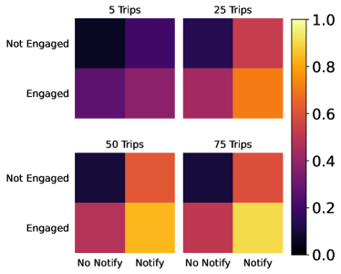
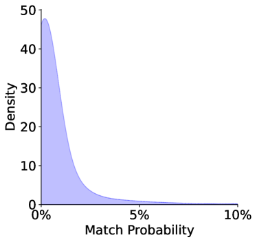
To apply the food rescue scenario to rmabs, we compute aggregate transition probabilities for volunteers through clustering. Each volunteer in the food rescue performs a certain number of trips, and we use this information to construct clusters. We ignore volunteers who have performed 1 or 2 trips, as those volunteers have too little information to construct transition functions for. We construct 100 clusters of roughly equal size, where each cluster consists of volunteers who perform a certain number of trips; for example, the 1st cluster consists of all volunteers who perform 3 trips, and the 90th cluster is those who perform 107-115 trips. From this, we compute transition probabilities by letting the state (which represents engagement) denote whether a volunteer has completed a trip in the past two weeks. We then see if completing a trip in the current two weeks impacts the chance that they complete a trip in the next two weeks. We use this as a proxy for engagement due to the lack of ground truth information on whether a volunteer is truly engaged. We average this over all volunteers in a cluster and across time periods to compute transition probabilities. We present examples of such transition probabilities in Figure 4. To compute the corresponding match probabilities for each volunteer, we compute the fraction of notifications they accept, across all notifications seen. This way, each arm corresponds to a cluster of volunteers, with a transition probability and match probability. We compute match probabilities on a per-volunteer basis so that multiple arms can have the same transition probability (corresponding to volunteers being in the same cluster) while differing in match probability. Such a situation corresponds to the real world as well; not all volunteers who complete between 107-115 trips have the same match probability.
We analyze the distribution of match probabilities for each volunteer, across all trips that they are notified for. We find that most volunteers accept less than 2% of the trips they’ve seen, while a few volunteers answer more than 10% (Figure 4). We note the difference between our two scenarios: notifications and phone calls. For notifications, we consider all volunteers and notify a large fraction of these volunteers, while for phone calls, we consider only volunteers who have completed more than 100 trips, as they generally have a higher match probability. We then cluster those volunteers into 20 groups and similarly compute transition probabilities. We do this because food rescue organizations target more active volunteers when making phone calls due to the limited number of phone calls that can be made.
Appendix E Vanilla MCTS Experiments
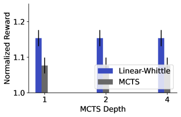
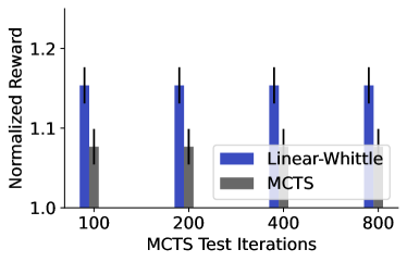
To understand the impact of our choice of hyperparameters for the MCTS baseline algorithm, we vary the depth of the MCTS search, along with the number of iterations. We vary the depth of MCTS in (while setting the iterations to ), and we vary the number of iterations run for MCTS in (while searching up to depth ). For all runs, we let and for the Max reward.
In Figure 5, we see that increasing MCTS depth only lowers performance, while increasing the number of iterations MCTS is run for increases performance. This is due to the stochasticity in rewards as the depth of exploration increases; there are possible combinations of states, making exploration difficult. We find that for any combination of iterations and depth, the performance of MCTS lags significantly behind Linear-Whittle. While running MCTS for additional iterations would be helpful, this comes at a cost of time, so we run MCTS for iterations throughout our experiments to balance these.
Appendix F Deep Q Networks
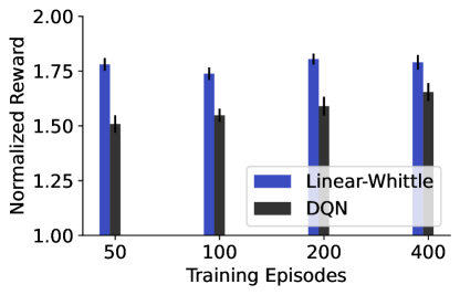
We compare the performance of our reinforcement learning baseline (dqn) to the Linear-Whittle policy as we vary the number of epochs that the dqn is trained for. We vary the number of train epochs in and plot our results in Figure 6. We see that increasing the number of iterations does not provide a big advantage in performance; this is because dqn fails to learn past epochs, and so additional training steps do not lead to much better performance. Moreover, we see that, no matter the selection of train iterations, dqn performs worse than Linear-Whittle. We believe the reason for this is the stochasticity in the dataset; because the number of actions is large, it becomes difficult to learn state values in this scenario, which leads to the poor performance of dqn.
Appendix G Synthetic Transitions
Throughout our experiments, we sample synthetic transitions, with a maximum probability for of ; we vary the value of to understand if this impacts the performance of policies. We vary , and evaluate the performance of our policies on the Max reward.
We find that, across all values of , the MCTS Shapley-Whittle policy performs best. We find large gaps between MCTS Shapley-Whittle and Linear-Whittle for small ; in these scenarios, the transitions are more stochastic, leading to greater impact from MCTS Shapley-Whittle. However, regardless of the choice of , our conclusion remains that Iterative and MCTS Shapley-Whittle policies outperform other alternatives.
Appendix H Other Constructions of Transitions
We investigate whether situations detailed in Lemma 8 can be tackled by adaptive algorithms. We construct a situation for the Max reward where transitions are and ; pulling an arm always leads to , and otherwise, arms stay in their current state. We design such a situation to see whether adaptive policies can perform well in situations where index-based policies are proven to perform poorly. We let the values , then let the other choices of . We do this to encourage arms to be pulled one at a time, rather than pulling and together. In Figure 8, we compare the performance of policies in this situation and see that Iterative Shapley-Whittle significantly outperforms all other policies when , and that MCTS Linear- and Shapley-Whittle outperform all other policies when . When , we see that all non-adaptive Whittle policies achieve similar performance, demonstrating the need for adaptive policies.
Appendix I Other Combinations of Arms and Budget
More arms
We evaluate the performance of policies when or and plot this in Figure 9. We run Iterative Shapley-Whittle, MCTS Linear-Whittle, and MCTS Shapley-Whittle policies for and refrain from running them when due to the time needed. We find that MCTS Shapley-Whittle policies perform better than alternatives, and that they perform significantly better than Linear-Whittle policies. The results with and confirm the trends from Section 6.1 even when the number of arms is large.
Weighting Individual and Global Rewards
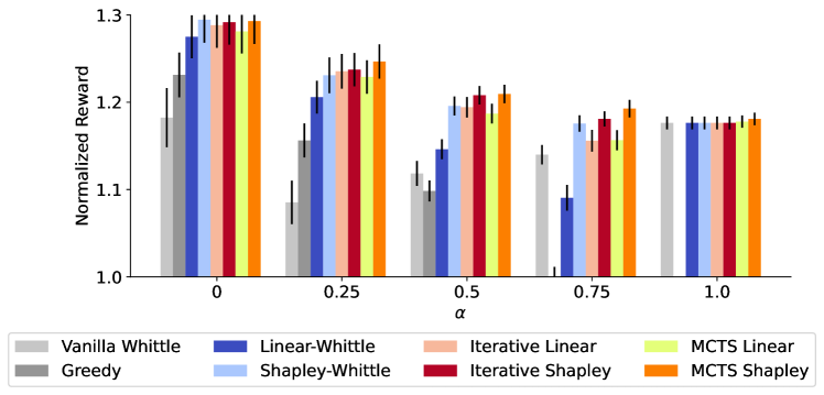
Throughout our experiments, we weight the impact of the global reward, , and the individual reward, , equally. We evaluate the impact of various weighting factors so that . By default, throughout our experiments, so we vary and evaluate the reward for baselines and our policies on the maximum reward.
In Figure 10, we see that, regardless of the choice of , our policies outperform baselines. We additionally see that the Shapley-Whittle and Iterative Shapley-Whittle perform well across the choices of , implying that the results we found with are not limited to one choice of .
Varying Budget
Throughout our experiments, we let the budget, , so we analyze the impact of varying when fixing . We vary , and note that with or , all policies perform the same (as all or no arms are selected). We see that, across all choices of budget, Linear-Whittle performs worse than all other policies (Figure 11). Moreover, we see again that regardless of the choice of , MCTS Shapley-Whittle is the best policy.
Appendix J Food Rescue More Arms
In addition to the experiments in Section 6.2, we evaluate the impact of increasing the number of arms in food rescue on the performance of various policies. We consider a situation with and , for the notification scenario, and another situation with and , which corresponds to the phone calls scenario. We plot both situations in Figure 12, and we see that all policies perform similarly in both of these situations. When the number of arms is this large, all policies will select the top arms as arms are likely to have a large match probability due to the sheer number of arms. We can differentiate between policies in the notification scenario, where Shapley-Whittle policies perform better than Linaer-Whittle policies, but in the phone calls settings, all policies perform similarly. Additionally, due to the large budget, the match probability will be large, so policies should focus on engagement in this scenario. In reality, the choice of whether to use pre-computed index policies or adaptive policies depends on the time available, the size of the problem, and the structure of the reward.
Appendix K Proofs of Problem Difficulty
Theorem 1.
The restless multi-armed bandit with global rewards is PSPACE-Hard.
Proof.
We reduce rmab to rmab-g. Note that rmab-g aims to maximize
| (9) |
Consider an rmab instance with reward . We can construct an instance of rmab-g with and with . Therefore, we have reduced rmab to rmab-g. Because rmab is PSPACE-Hard [26], rmab-g is as well. ∎
Theorem 2.
No polynomial time algorithm can achieve better than a approximation to the restless multi-armed bandit with global rewards problem.
Proof.
Consider any submodular function and a cardinality constraint . Unless , maximizing with a cardinality constraint can only be approximated up to a factor of [33]. Next, we will show that we can reduce submodular maximization to rmab-g.
For a given submodular function , we construct an instance of rmab-g with . Let , where is the vector of 1s. Finally let , so that all arms are in state for timesteps . Let if , and let otherwise. Note that only at time can you achieve any reward, as afterwards, .
The optimal solution to the rmab-g problem is the action, that maximizes subject to the constraint, . Note that this is the same as the cardinality constraint for submodular maximization, , along with the function of interest, . Therefore, if we can efficiently solve rmab-g, then we can efficiently solve the original submodular maximization problem in . Because we cannot do better than a approximation to the submodular maximization problem in polynomial time, we cannot do better than a approximation to the rmab-g problem. ∎
Lemma 9.
Let be a set of transition functions, , where is the number of arms. Let . Let for some policy , and let be the optimal policy. Let . If is monotonic in and for any , then is monotonic in
Proof.
We construct by stepping through inductive steps in value iteration, and showing that the monotonicity property is preserved throughout these steps. We note that performing Value iteration from any initialization results in the optimal policy,
Let represent the value for iteration of Value iteration, and let be the value function for iteration .
We initialize for any , and note that the initialization should not impact the process.
Running an iteration of value iteration leads , so that .
Base Case: Initially, . Next consider any two states, and , so that .
Here implies that .
Let .
Then .
Therefore, is monotonic.
Inductive Hypothesis: Assume that is monotonic in .
Next, we will prove that .
Here is the vector with 1 at location and 0 everywhere else.
Before proving this, we will first show that this implies monotonicity for any two states . Suppose that . Then consider some pair of states, . Because , if , then we can write for some set . If , then
Therefore, this implies that
| (10) |
We get this by expanding into a telescoping series.
Because each term in the sum is non-negative, the whole sum is non-negative.
Next we prove our original statement: .
We first expand for some , where .
We note that
Therefore:
| (11) |
We note that due to the monotonicity of with fixed .
Let be the set of 0-1 vectors of length so that if then .
Additionally, let .
We note that
Let be the vector of all 1s except at .
Let be the element-wise minimum operator.
Then sets while leaving other indices unchanged.
Because transition probabilities add to one,
Next:
The second step splits the sum into transitions for states with and those with . The final step applies the inductive hypothesis and noting that . ∎
Lemma 10.
Let be a set of transition functions, , where is the number of arms. Let . Let for some policy , and let be the optimal policy. Let . If is submodular in both and , is submodular in , and for any , then is submodular in .
Proof.
We similarly construct through induction in the value iteration steps.
Base Case: We start with the base case: , which is submodular by assumption.
Inductive Hypothesis: Again let be the value function at step of value iteration. We assume that is submodular, and aim to prove that .
We note that this is an equivalent definition of submodularity [34].
Now, consider .
The sum of submodular functions is submodular and note that .
We note that the first term is submodular by assumption, so we focus on proving the submodularity of .
Let be the set of 0-1 vectors of length so that if then , and let ; note the different definition of from the previous proof.
Finally, let , then we can write the following:
The last step arises because , are all non-negative, and the inductive hypothesis. ∎
Theorem 3.
Consider an rmab-g instance . Let and let be the optimal policy. Let . Suppose , , monotonic and submodular in and , and submodular in . Then with oracle access to we can compute in time so .
Proof.
We first demonstrate that is submodular and monotonic in .
Prior work demonstrates that monotonic submodular function can be approximated within an approximation factor of with evaluations of the function, so all that remains is to demonstrate submodularity [12].
We note that , and that is both monotonic and submodular in .
Therefore, we demonstrate that is monotonic and submodular in .
Let for fixed .
We start by demonstrating monotonicity.
First, let , and by assumption, .
Then:
The last steps follows from the monotonicity of , which was proven in Lemma 9.
Next, we prove submodularity of , by showing that . That is
The last line follows from the submodularity of , as proven in Lemma 10. Therefore, we have shown that is submodular, which completes the proof. ∎
Appendix L Proofs of Index-Based Bounds
L.1 Lower Bounds
Theorem 4.
For any fixed set of transitions, , let for some . For an rmab-g , let , and let the induced linear rmab be . Let be the Linear-Whittle policy, and let . Define as
| (12) |
If the induced linear rmab is irreducible and indexable with the uniform global attractor property, then asymptotically in for any set of transitions, .
Proof.
By the definition of the minimum, .
Additionally, note that .
This holds because .
So, by submodularity of .
We compare the linearized reward to the submodular reward for the set of actions played by the Linear-Whittle policy .
Let the actions be .
If we play for iterations, then:
| (13) |
Next, consider the following induced rmab with . By assumption, our relaxed rmab is indexable, irreducible, and has a global attractor. In this scenario, prior work [2] states that the Whittle index is asymptotically optimal.
For this relaxed rmab problem, we note that the Whittle Index solution corresponds exactly to the Linear-Whittle policy, . That is
| (14) |
Then, asymptotically,
∎
Theorem 5.
For any fixed set of transitions, , let for some . For an rmab-g , let , and let the induced Shapley rmab be . Let be the Shapley-Whittle policy, and let . Define as
| (15) |
If the induced Shapley rmab is irreducible and indexable with the uniform global attractor property, then asymptotically in for any choice of transitions, .
Proof.
Corollary 5.1.
Consider an rmab-g instance with a monotonic, submodular reward function , and let be the Linear-Whittle policy. Let and for some . Then for any transitions .
Proof.
By Theorem 4, we know that . We next show that .
For a monotonic, submodular function, , .
Next, applying this to our global reward function, for a fixed state , we note that .
Next, by construction, .
Additionally,
Next, for any state , .
Combining the bounds on and , gives that for any state ,
| (17) |
Therefore, , completing our proof.
∎
L.2 Upper Bounds
Theorem 6.
Let . For a set of transitions , let and . Define as follows:
| (18) |
Then there exists some transitions, , and initial state , so that
Proof.
We prove this by constructing such a set of transitions such that . Let . Next, let be the identity transition; for any . Under these transitions, all arms stay in the state for all time periods .
Because the state is constant, the set of actions played, is constant across time periods (as the Linear-Whittle algorithm is deterministic). We next show that the Linear-Whittle policy plays the action . We note that all arms have the same transitions; therefore, arms are played in order of , as each arm is predicted to receive a reward . This is because Linear-Whittle aims to maximize the sum of marginal rewards, and when the transitions are homogeneous, chooses the largest values for . In other words, the Linear-Whittle policy chooses an action, so that
| (19) |
Finally, we observe that the optimal action to play is . The ratio of rewards between these two actions is exactly , and therefore, ∎
Theorem 7.
Let . For a set of transitions and initial state , let and . Let be:
| (20) |
Then there exists some transitions, and initial state so that
Proof.
We follow the same strategy as the proof for the Linear-Whittle case and construct a set of transition probabilities so that . Again, let and be the identity transition. By the same reasoning as Theorem 6, the Shapley-Whittle policy will play the action ; the Linear- and Shapley-Whittle situations are analogous, with the only difference being that Shapley-Whittle assumes each arm receives a reward of instead of . The optimal action played receives a reward of , so that the ratio between the reward of the Shapley-Whittle policy and optimal is
| (21) |
This is exactly when . ∎
Lemma 8.
Define an index-based policy as any policy that can be described through a function , such that in state , the policy, selects the largest values of , where such a function is evaluated for each arm. Then index-based algorithms will achieve a discounted reward approximation ratio no better than
Proof.
Consider an arm system, with . Suppose our reward is . Next, define the transition probabilities for all arms as follows: and ; if an arm is pulled, then the arm will transition to state 0, and otherwise, the arm remains in its current state.
Then note that because of symmetry between the arms, is identical, as is symmetric across arms, and and is the same across arms. Moreover, because there are arms, all arms will be selected in the first time step. Therefore, any index-based strategy will lead to a reward of . However, selecting arm in timestep instead leads to rewards in each of the timesteps, leading to a total reward of when . Applying the geometric sum formula reveals that this is a approximation. ∎