On a perturbation analysis of Higham squared maximum Gaussian elimination growth matrices

Alan Edelman Department of Mathematics, Massachusetts Institute of Technology, Cambridge, MA, 02139 USA. edelman@mit.edu John Urschel urschel@mit.edu  and  Bowen Zhu bowenzhu@g.harvard.edu School of Engineering and Applied Sciences, Harvard University, Cambridge, MA, 02138 USA.
Abstract.

Gaussian elimination is the most popular technique for solving a dense linear system. Large errors in this procedure can occur in floating point arithmetic when the matrix’s growth factor is large. We study this potential issue and how perturbations can improve the robustness of the Gaussian elimination algorithm. In their 1989 paper, Higham and Higham characterized the complete set of real n by n matrices that achieves the maximum growth factor under partial pivoting. This set of matrices serves as the critical focus of this work. Through theoretical insights and empirical results, we illustrate the high sensitivity of the growth factor of these matrices to perturbations and show how subtle changes can be strategically applied to matrix entries to significantly reduce the growth, thus enhancing computational stability and accuracy.

2020 Mathematics Subject Classification:
Primary 65F05, 15A23.

1. Introduction to Partial Pivoting Growth

It is well-known, even to beginning students in engineering and science, that the most popular method for solving the dense linear system $Ax=b$ for $x$ is Gaussian elimination. Indeed, this method, employed using partial pivoting, is widely available through interfaces from high level languages such as Julia [1], Mathematica [12], Matlab [11], Python NumPy [7], R [13], etc. Error estimates for the stability of the Gaussian elimination algorithm in floating point arithmetic are governed by the bits of precision used, the condition number of the matrix, and the growth factor (i.e., the largest magnitude entry encountered during the Gaussian elimination algorithm) [5, Theorem 3.3.2]. Many researchers have studied and continue to study the question of why Gaussian elimination with partial pivoting has been so very effective [4, 8, 9, 10, 14, 15, 16, 17]. In contrast to complete pivoting, where the existence of matrices with even super-linear growth remains an open problem [2, 3, 6], it has been known since Wilkinson’s classic text The Algebraic Eigenvalue Problem [18, p.212] that, for partial pivoting, the growth factor is bounded above by $2^{n-1}$ and that this quantity can be achieved by the matrix

$$A=\begin{pmatrix}[r]1&0\phantom{.}&\cdots&0&1\\ -1&\ddots&\ddots&\vdots&\vdots\\ \vdots&\ddots&1&0&1\\ -1&\cdots&-1&1&1\\ -1&\cdots&-1&-1&1\end{pmatrix}.$$ (1.1)

Much later, Higham and Higham (from now on denoted Higham222We denote “Higham and Higham” as Higham2, to be read as “Higham squared,” yet we realize this has the appearance of a footnote, so for readers who saw it this way, we have included this footnote. ) identified the complete set of $n$ by $n$ real matrices that achieve the maximal growth of $2^{n-1}$ [9]. We call such matrices Higham2 matrices (see Proposition 2.2 for a description). A scalar quantity of interest is the last pivot of a Higham2 matrix, which is a differentiable function of the matrix entries. We can therefore ask for the gradient of this last pivot or, even better, to have a full (non-infinitesimal) perturbation analysis of the last pivot (for Gaussian elimination without pivoting). We provide such a perturbation analysis in Theorem 2.3. The last pivot is an ideal quantity to measure in order to understand the growth factor, as every entry of $U$ is the last pivot of the LU factorization of some submatrix of $A$. We observe that generically, large growth does not last very long in the sense that often a small perturbation can dramatically reduce a large pivot. We have a mental image that the Higham2 matrices live on a kind of “ridge” that one can easily fall off of. This picture is consistent with the smoothed analysis of Sankar, Spielman, and Teng [14]. The structure of the Higham2 matrices provide an ideal setting to better understand the ridge and its profile. Perhaps unsurprisingly, not all directions of descent are created equal. We provide numerical experiments (in Section 3) to visualize the effects of perturbing Higham2 matrices and confirm the conclusions gleaned from the theoretical results of Section 2.

2. Entrywise Perturbations & Higham2 Matrices

Here we provide mathematical estimates for the effects of entrywise perturbations on the last pivot of the LU factorization (without pivoting) of a matrix (Lemma 2.1), recall a characterization of Higham2 matrices (Proposition 2.2), and consider the effects of entrywise perturbations on this class (Theorem 2.3, Corollaries 2.4 & 2.5). These theoretical results give insight into the experimental observations in Section 3.

Lemma 2.1.

Let

$$A=\begin{pmatrix}\hat{L}&0\\ \bm{\ell}^{T}&1\end{pmatrix}\begin{pmatrix}\hat{U}&\bm{u}\\ 0&p\end{pmatrix}\in\mathrm{GL}_{n}(\mathbb{R}),$$

where $\hat{L}\in\mathrm{SL}_{n-1}(\mathbb{R})$ is lower unitriangular, $\hat{U}\in\mathrm{GL}_{n-1}(\mathbb{R})$ is upper triangular, and $\bm{\ell},\bm{u}\in\mathbb{R}^{n-1}$. Then the LU factorization, if it exists, of $A+\epsilon\,\bm{e}_{i}\bm{e}_{j}^{T}$, where $\bm{e}_{i}$ is the $i^{th}$ standard basis vector, has last pivot

$$p^{(i,j)}_{\epsilon}=p+\epsilon\frac{(\hat{U}^{-1}\bm{u})_{j}(\bm{\ell}^{T}\hat{L}^{-1})_{i}}{1+\epsilon(\hat{L}\hat{U})^{-1}_{ji}}\qquad\text{for}\quad i,j<n,$$

$p^{(i,n)}_{\epsilon}=p-\epsilon(\bm{\ell}^{T}\hat{L}^{-1})_{i}$ for $i<n$, $p^{(n,j)}_{\epsilon}=p-\epsilon(\hat{U}^{-1}\bm{u})_{j}$ for $j<n$, and $p^{(n,n)}_{\epsilon}=p+\epsilon$.

Proof.

We first consider the case $i,j<n$. The last pivot is a ratio of determinants

$$p^{(i,j)}_{\epsilon}=\frac{\det(A+\epsilon\,\bm{e}_{i}\bm{e}_{j}^{T})}{\det(\hat{L}\hat{U}+\epsilon\,\bm{\hat{e}}_{i}\bm{\hat{e}}_{j}^{T})}=\frac{\det(A)}{\det(\hat{L}\hat{U})}\,\bigg{(}\frac{1+\epsilon\bm{e}_{j}^{T}A^{-1}\bm{e}_{i}}{1+\epsilon\bm{\hat{e}}_{j}^{T}(\hat{L}\hat{U})^{-1}\bm{\hat{e}}_{i}}\bigg{)}=p\bigg{(}\frac{1+\epsilon A^{-1}_{ji}}{1+\epsilon(\hat{L}\hat{U})^{-1}_{ji}}\bigg{)},$$

where $\bm{\hat{e}}_{i}$ is the $i^{th}$ standard basis vector in $\mathbb{R}^{n-1}$. The matrix $A^{-1}$ has block form

$$A^{-1}=\begin{pmatrix}\hat{U}^{-1}&-p^{-1}\hat{U}^{-1}\bm{u}\\ 0&p^{-1}\end{pmatrix}\begin{pmatrix}\hat{L}^{-1}&0\\ -\bm{\ell}^{T}\hat{L}^{-1}&1\end{pmatrix}=\begin{pmatrix}(\hat{L}\hat{U})^{-1}+p^{-1}\hat{U}^{-1}\bm{u}\bm{\ell}^{T}\hat{L}^{-1}&-p^{-1}\hat{U}^{-1}\bm{u}\\ -p^{-1}\bm{\ell}^{T}\hat{L}^{-1}&p^{-1}\end{pmatrix},$$

and so $A^{-1}_{ji}=(\hat{L}\hat{U})_{ji}^{-1}+p^{-1}(\hat{U}^{-1}\bm{u})_{j}(\bm{\ell}^{T}\hat{L}^{-1})_{i}$. Therefore,

$$p^{(i,j)}_{\epsilon}-p=p\bigg{[}\frac{1+\epsilon A^{-1}_{ji}}{1+\epsilon(\hat{L}\hat{U})^{-1}_{ji}}-1\bigg{]}=\frac{\epsilon p(A^{-1}_{ji}-(\hat{L}\hat{U})^{-1}_{ji})}{1+\epsilon(\hat{L}\hat{U})^{-1}_{ji}}=\frac{\epsilon(\hat{U}^{-1}\bm{u})_{j}(\bm{\ell}^{T}\hat{L}^{-1})_{i}}{1+\epsilon(\hat{L}\hat{U})^{-1}_{ji}}.$$

When $i=n$ or $j=n$, $\displaystyle{p^{(i,j)}_{\epsilon}=\frac{\det(A+\epsilon\,\bm{e}_{i}\bm{e}_{j}^{T})}{\det(\hat{L}\hat{U})}=p(1+\epsilon A^{-1}_{ji}).}$ Noting that $A_{jn}^{-1}=-p^{-1}(\hat{U}^{-1}\bm{u})_{j}$ for $j<n$, $A_{ni}^{-1}=-p^{-1}(\bm{\ell}^{T}\hat{L}^{-1})_{i}$ for $i<n$, and $A_{nn}^{-1}=p^{-1}$ completes the proof. ∎

We recall the following characterization of Higham2 matrices from the original paper of Higham and Higham [9], where we have slightly adjusted the normalization and notation to suit our needs.

Proposition 2.2.

[9, Theorem 2.2] Every matrix $A\in\mathrm{GL}_{n}(\mathbb{R})$, $\|A\|_{\max}=1$, with growth factor under partial pivoting equal to $2^{n-1}$ is of the form

$$DPA=\begin{pmatrix}\hat{L}&0\\ -\bm{1}^{T}&1\end{pmatrix}\begin{pmatrix}\hat{U}&\bm{u}\\ 0&2^{n-1}\end{pmatrix}=\begin{pmatrix}\hat{L}\hat{U}&\bm{1}\\ -\bm{1}^{T}\hat{U}&1\end{pmatrix},$$ (2.1)

where $D\in\mathrm{GL}_{n}(\mathbb{R})$ is a $\pm 1$ diagonal matrix, $P\in\mathrm{GL}_{n}(\mathbb{R})$ is a permutation matrix associated with a partial pivoting of $A$, $\hat{L}\in\mathrm{GL}_{n-1}(\mathbb{R})$ is lower unitriangular with $\hat{L}_{ij}=-1$ for all $i>j$, $\bm{1}$, $\bm{u}=(1,2,...,2^{n-2})^{T}\in\mathbb{R}^{n-1}$, and $\hat{U}\in\mathrm{GL}_{n-1}(\mathbb{R})$ is upper triangular, with entries satisfying $\|\hat{L}\hat{U}\|_{\max}\leq 1$ and $\|\bm{1}^{T}\hat{U}\|_{\infty}\leq 1$.

Applying Lemma 2.1 to Higham2 matrices (described in Proposition 2.2) gives the following theorem.

Theorem 2.3.

Let $A\in\mathrm{GL}_{n}(\mathbb{R})$, $\|A\|_{\max}=1$, be a Higham2 matrix of the form in Equation 2.1 with $P=D=I$. Then the LU factorization, if it exists, of $A+\epsilon\,\bm{e}_{i}\bm{e}_{j}^{T}$ has last pivot

$$p_{\epsilon}^{(i,j)}=\begin{cases}\displaystyle{\frac{1}{2^{1-n}+\epsilon\,2^{-i}\sum_{\ell=1}^{n-j}2^{-\ell}\hat{U}_{j,n-\ell}^{-1}}}&\qquad\text{for}\quad i<j<n\\[12.91663pt] \displaystyle{\frac{1+\tfrac{1}{2}\epsilon\,(\hat{U}_{ji}^{-1}-\sum_{\ell=1}^{i-j}2^{-\ell}\hat{U}_{j,i-\ell}^{-1})}{2^{1-n}+\epsilon(2^{1-n}\hat{U}_{ji}^{-1}+2^{-i}\sum_{\ell=1}^{n-i-1}2^{-\ell}\hat{U}_{j,n-\ell}^{-1})}}&\qquad\text{for}\quad j\leq i<n\\[4.30554pt] \end{cases}\quad,$$ (2.2)

$p_{\epsilon}^{(i,n)}=2^{n-1}(1+\epsilon\,2^{-i})$ for $i<n$, $p_{\epsilon}^{(n,j)}=2^{n-1}(1-\epsilon\sum_{\ell=1}^{n-j}2^{-\ell}\hat{U}_{j,n-\ell}^{-1})$ for $j<n$, and $p_{\epsilon}^{(n,n)}=2^{n-1}+\epsilon$.

Proof.

By Proposition 2.2, $A=\begin{pmatrix}\hat{L}&0\\ -\bm{1}^{T}&1\end{pmatrix}\begin{pmatrix}\hat{U}&\bm{u}\\ 0&2^{n-1}\end{pmatrix}$, where $\hat{L}\in\mathrm{SL}_{n-1}(\mathbb{R})$ is lower unitriangular with $\hat{L}_{ij}=-1$ for all $i>j$, $\bm{u}=(1,2,...,2^{n-2})^{T}$, and $\hat{U}\in\mathrm{GL}_{n-1}(\mathbb{R})$ is upper triangular. The matrix $\hat{L}$ has a simple structure, and its inverse has entries given by $\hat{L}^{-1}_{ij}=\phi(i-j)$, where $\phi(k)$ equals zero for $k<0$, one for $k=0$, and $2^{k-1}$ for $k>0$. Therefore,

$$(\bm{1}^{T}\hat{L}^{-1})_{i}=\sum_{k=i}^{n-1}\phi(k-i)=2^{n-i-1}\qquad\text{and}\qquad(\hat{L}\hat{U})_{ji}^{-1}=\sum_{k=i}^{n-1}\phi(k-i)\hat{U}_{jk}^{-1}=\hat{U}_{ji}^{-1}+\sum_{k=i+1}^{n-1}2^{k-i-1}\hat{U}_{jk}^{-1}.$$

Applying Lemma 2.1 to $A$ and noting that $(\hat{U}^{-1}\bm{u})_{j}=\sum_{k=j}^{n-1}2^{k-1}\hat{U}^{-1}_{jk}$, we have $p_{\epsilon}^{(n,n)}=2^{n-1}+\epsilon$, $p_{\epsilon}^{(i,n)}=2^{n-1}(1+\epsilon\,2^{-i})$ for $i<n$, $p_{\epsilon}^{(n,j)}=2^{n-1}(1-\epsilon\sum_{\ell=1}^{n-j}2^{-\ell}\hat{U}_{j,n-\ell}^{-1})$ for $j<n$, and

$$p_{\epsilon}^{(i,j)}=2^{n-1}-\frac{\epsilon 2^{n-i-1}\sum_{k=j}^{n-1}2^{k-1}\hat{U}^{-1}_{jk}}{1+\epsilon(\hat{U}_{ji}^{-1}+\sum_{k=i+1}^{n-1}2^{k-i-1}\hat{U}_{jk}^{-1})}\qquad\text{for}\quad i,j<n.$$

When $i<j<n$, $\hat{U}_{ji}^{-1}=0$ and $\sum_{k=i+1}^{n-1}2^{k-i-1}\hat{U}_{jk}^{-1}=\sum_{k=j}^{n-1}2^{k-i-1}\hat{U}^{-1}_{jk}$, and so $p_{\epsilon}^{(i,j)}$ equals $(2^{1-n}+\epsilon\,2^{-i}\sum_{\ell=1}^{n-j}2^{-\ell}\hat{U}_{j,n-\ell}^{-1})^{-1}$. Finally, in the case $j\leq i<n$, we have

$$p_{\epsilon}^{(i,j)}=\frac{1+\tfrac{1}{2}\epsilon\,(\hat{U}_{ji}^{-1}-\sum_{\ell=1}^{i-j}2^{-\ell}\hat{U}_{j,i-\ell}^{-1})}{2^{1-n}+\epsilon(2^{1-n}\hat{U}_{ji}^{-1}+2^{-i}\sum_{\ell=1}^{n-i-1}2^{-\ell}\hat{U}_{j,n-\ell}^{-1})}.$$

Equation 2.2 of Theorem 2.3 deserves a number of observations. First, we note a connection between the rate at which $p_{\epsilon}^{(i,j)}$ decreases and the condition number of the matrix: if the last pivot under $\epsilon$ perturbation is much smaller than $1/|\epsilon|$, then $A$ is ill-conditioned.

Corollary 2.4.

Let $A\in\mathrm{GL}_{n}(\mathbb{R})$, $\|A\|_{\max}=1$, be a Higham2 matrix of the form in Equation 2.1 with $P=D=I$. If $|\epsilon|<1$ and $\sqrt{n}<|p_{\epsilon}^{(i,j)}|<2^{n-5}$, then $\kappa_{2}(A)=\|A\|_{2}\|A^{-1}\|_{2}\geq\sqrt{n}\,\big{|}3\epsilon p_{\epsilon}^{(i,j)}\big{|}^{-1}$.

Proof.

Let $|\epsilon|<1$ and $\sqrt{n}<|p_{\epsilon}^{(i,j)}|<2^{n-5}$ for some $i,j$. We first relate $\kappa_{2}(A)$ to the entries of $U^{-1}$:

$$\|A\|_{2}\|A^{-1}\|_{2}\geq\|A\mathbf{e}_{n}\|_{2}\|A^{-1}\|_{2}=\sqrt{n}\max_{y\neq 0}\frac{\|U^{-1}y\|_{2}}{\|Ly\|_{2}}\geq\sqrt{n}\max_{\ell}\frac{\|U^{-1}e_{n-\ell}\|_{2}}{\|Le_{n-\ell}\|_{2}}\geq\max_{k,\ell}\frac{\sqrt{n}\,|U^{-1}_{k,n-\ell}|}{\sqrt{\ell+1}}.$$

What remains is to show that $|U^{-1}_{k,n-\ell}|\geq\sqrt{\ell+1}\,\big{|}3\epsilon p_{\epsilon}^{(i,j)}\big{|}^{-1}$ for some $k,\ell$. We proceed by contradiction. If this is not the case, then

$$\left|\epsilon\sum_{\ell=1}^{k}\frac{\hat{U}_{j,n-\ell}^{-1}}{2^{\ell}}\right|<\frac{1}{\big{|}p_{\epsilon}^{(i,j)}\big{|}}\sum_{\ell=1}^{\infty}\frac{\sqrt{\ell+1}}{3\times 2^{\ell}}<\frac{0.57}{\big{|}p_{\epsilon}^{(i,j)}\big{|}}\quad\text{and}\quad\left|\epsilon\,(\hat{U}_{ji}^{-1}-\sum_{\ell=1}^{i-j}2^{-\ell}\hat{U}_{j,i-\ell}^{-1})\right|<\sum_{\ell=0}^{\infty}\frac{1}{3\times 2^{\ell}}=\frac{2}{3}.$$

These two bounds, combined with the formulae of Theorem 2.3, lead to a contradiction for all choices of $(i,j)$. For example, if $j\leq i<n$, then

$$\big{|}p_{\epsilon}^{(i,j)}\big{|}\geq\frac{1-\tfrac{1}{2}\left|\epsilon\,(\hat{U}_{ji}^{-1}-\sum_{\ell=1}^{i-j}2^{-\ell}\hat{U}_{j,i-\ell}^{-1})\right|}{2^{1-n}+\left|\epsilon(2^{1-n}\hat{U}_{ji}^{-1}+2^{-i}\sum_{\ell=1}^{n-i-1}2^{-\ell}\hat{U}_{j,n-\ell}^{-1})\right|}>\frac{2/3}{2^{1-n}+0.57/\big{|}p_{\epsilon}^{(i,j)}\big{|}}>\frac{2/3}{2^{-4}+0.57}\,\big{|}p_{\epsilon}^{(i,j)}\big{|},$$

a contradiction. The remaining cases are similar, and are left to the reader. ∎

Now, let us restrict our attention to the case $i<j<n$, with $i$ relatively small. As long as $\epsilon\,2^{-i}\sum_{\ell=1}^{n-j}2^{-\ell}\hat{U}_{j,n-\ell}^{-1}$ is not exponentially small in $n$, $p_{\epsilon}^{(i,j)}$ is approximately $2^{i}\,(\epsilon\,\sum_{\ell=1}^{n-j}2^{-\ell}\hat{U}_{j,n-\ell}^{-1})^{-1}$. One would expect this to be the case for “most” Higham2 matrices when $\epsilon$ is only polynomially small, though exceptions certainly exist (e.g., the Wilkinson matrix $\hat{U}=I$). This intuition is supported by experimental results in Section 3. The case $i=1$ and $j=n-1$ is particularly striking, and gives guaranteed improvement for all Higham2 matrices.

Corollary 2.5.

Let $A\in\mathrm{GL}_{n}(\mathbb{R})$, $\|A\|_{\max}=1$, be a Higham2 matrix of the form in Equation 2.1 with $P=D=I$. Then

$$|p^{(1,n-1)}_{\epsilon}|\leq\frac{4+o_{n}(1)}{|\epsilon|},\qquad\text{where}\qquad|o_{n}(1)|<2^{-(n-6)}|\epsilon|^{-1}\;\text{for}\;|\epsilon|>2^{-(n-4)}.$$ (2.3)
Proof.

By Equation 2.2,

$$p^{(1,n-1)}_{\epsilon}=\frac{4\hat{U}_{n-1,n-1}}{\epsilon+2^{-(n-3)}\hat{U}_{n-1,n-1}}=\frac{\hat{U}_{n-1,n-1}}{\epsilon}\bigg{(}4-\frac{2^{-(n-5)}\hat{U}_{n-1,n-1}}{\epsilon+2^{-(n-3)}\hat{U}_{n-1,n-1}}\bigg{)}.$$

Noting that $|\hat{U}_{n-1,n-1}|=\big{|}\big{[}(\hat{L}\hat{U})_{n-1,n-1}+(\bm{1}^{T}\hat{U})_{n-1}\big{]}/2\big{|}\leq 1$ gives the desired result. ∎

The entry $(1,n-1)$ is an example of a perturbation direction that always produces a small last pivot when $\epsilon$ is only polynomially small. Finally, we note that, while Lemma 2.1 and Theorem 2.3 apply only to the last pivot, this general framework holds for arbitrary entries of $U$, as every entry of $U$ is the last pivot of the LU factorization of some submatrix of $A$. For instance, Corollary 2.5 implies that a only polynomially small $\epsilon$ perturbation to the $(1,n-k)^{th}$ entry of a Higham2 matrix leads to $|U_{n-k+1,n}|\leq(4+o_{n}(1))/|\epsilon|$ for any fixed $k$ (with $n$ growing). In Section 3, we make use of the insights gained from Theorem 2.3 to suggest perturbations tailored to the most influential components of $A$, and compare their effect to perturbations applied uniformly to $A$.

3. Experimental Results

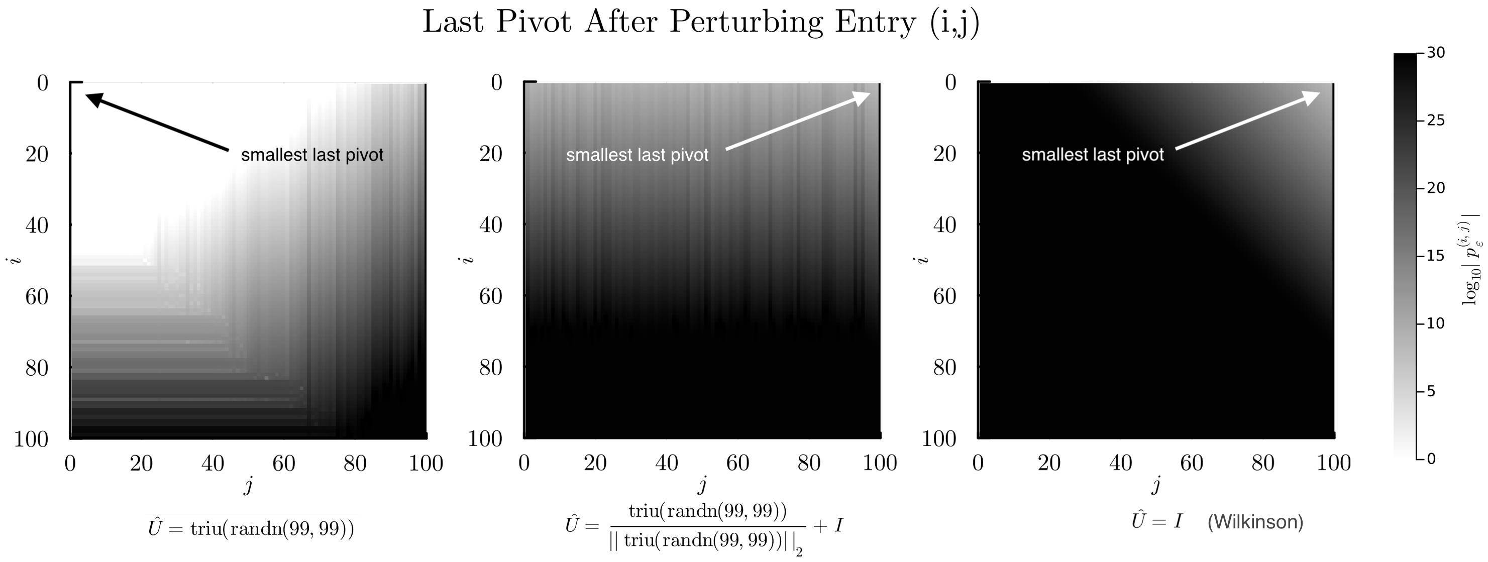
Here we perform two experiments, illustrated in Figures 1 and LABEL:fig:data. First, in Figure 1, we consider the effects of an $\epsilon=10^{-8}$ perturbation to the last pivot of Higham2 matrices of dimension $n=100$. Though $n=100$ is quite a small test-case, it is already more than sufficient for our purposes, as, in double precision, the last pivot is nearly equal to the inverse of machine epsilon squared. The heatmap on the left is of a Higham2 matrix generated by taking the $\hat{U}\in\mathrm{GL}_{n-1}(\mathbb{R})$ of Proposition 2.2 to have independent standard normal entries, scaled so that $\|A\|_{\max}=1$, the map on the right is of the Wilkinson matrix (see Equation 1.1), and the map in the middle is of a matrix in between the two (w.r.t. choice of $\hat{U}$). Perturbations in the top left portion of a random Higham2 matrix appear to be most impactful. This is consistent with Theorem 2.3 and the fact that the inverse of an upper triangular matrix with normal entries tends to have exponentially large entries (in $n$) near the upper-right corner. However, the Wilkinson matrix provides a clear reminder that this is not always the case. The inverse of $\hat{U}=I$ has zero entries above the diagonal, rendering perturbations to the top-left entries of $A$ relatively useless. Our results are also consistent with Inequality 2.3: perturbing the top-right $(1,n-1)$ entry with a sufficiently large $\epsilon$ is a reliable way to always decrease the last pivot size.

Refer to caption
Figure 1. The effects of an $\epsilon=10^{-8}$ perturbation at different entries of three $100\times 100$ Higham2 matrices for different choices of $\hat{U}$ ($\hat{U}=I$ is the Wilkinson matrix). We plot a heatmap for each, where the $(i,j)^{th}$ grid point is the value of $\log_{10}|p^{(i,j)}_{\epsilon}|$ (in exact arithmetic).

Of course, we are not merely interested in the last pivot, but in the quality of solution to $Ax=b$ we obtain using Gaussian elimination. Our theoretical and experimental results in Theorem 2.3, Corollary 2.5, and Figure 1 give key insights into the stability of the last pivot, with implications for the growth factor itself, as every entry of $U$ is the last pivot of a sub-matrix of $A$. In Figure LABEL:fig:data, we examine the effects of matrix perturbation on the numerical solution to $Ax=b$ for Higham2 matrices using Gaussian elimination with no pivoting. In the left plot, we observe that the ill-conditioning of a random Higham2 matrix is a major barrier to a reasonable solution. This is consistent with the theoretical observation that extremely fast decay in the last pivot implies ill-conditioning (Corollary 2.4). In both the middle and right plots, we observe that the perturbation to the first row is the superior strategy. It is quite possible that this observation holds more broadly than the class of maximum growth factor Higham2 matrices considered here, and that there may be benefits to considering perturbations tailored specifically to Gaussian elimination with partial pivoting.

Acknowledgements

This material is based upon work supported by the National Science Foundation under grant no. OAC-1835443, grant no. SII-2029670, grant no. ECCS-2029670, grant no. OAC-2103804, and grant no. PHY-2021825. We also gratefully acknowledge the U.S. Agency for International Development through Penn State for grant no. S002283-USAID. The information, data, or work presented herein was funded in part by the Advanced Research Projects Agency-Energy (ARPA-E), U.S. Department of Energy, under Award Number DE-AR0001211 and DE-AR0001222. The views and opinions of authors expressed herein do not necessarily state or reflect those of the United States Government or any agency thereof. This material was supported by The Research Council of Norway and Equinor ASA through Research Council project “308817 - Digital wells for optimal production and drainage”. Research was sponsored by the United States Air Force Research Laboratory and the United States Air Force Artificial Intelligence Accelerator and was accomplished under Cooperative Agreement Number FA8750-19-2-1000. The views and conclusions contained in this document are those of the authors and should not be interpreted as representing the official policies, either expressed or implied, of the United States Air Force or the U.S. Government. The U.S. Government is authorized to reproduce and distribute reprints for Government purposes notwithstanding any copyright notation herein. The third author’s masters thesis [19] contains some of the results presented here, as well as some additional analysis and figures.

References

  • [1] Jeff Bezanson, Alan Edelman, Stefan Karpinski, and Viral B Shah. Julia: A fresh approach to numerical computing. SIAM review, 59(1):65–98, 2017.
  • [2] Ankit Bisain, Alan Edelman, and John Urschel. A new upper bound for the growth factor in Gaussian elimination with complete pivoting. arXiv preprint arXiv:2312.00994, 2023.
  • [3] Alan Edelman and John Urschel. Some new results on the maximum growth factor in Gaussian elimination. SIAM Journal on Matrix Analysis and Applications, 45(2):967–991, 2024.
  • [4] Leslie V Foster. Gaussian elimination with partial pivoting can fail in practice. SIAM Journal on Matrix Analysis and Applications, 15(4):1354–1362, 1994.
  • [5] Gene H Golub and Charles F Van Loan. Matrix computations. JHU press, 2013.
  • [6] Nick Gould. On growth in Gaussian elimination with complete pivoting. SIAM Journal on Matrix Analysis and Applications, 12(2):354–361, 1991.
  • [7] Charles R. Harris, K. Jarrod Millman, Stéfan J. van der Walt, Ralf Gommers, Pauli Virtanen, David Cournapeau, Eric Wieser, Julian Taylor, Sebastian Berg, Nathaniel J. Smith, Robert Kern, Matti Picus, Stephan Hoyer, Marten H. van Kerkwijk, Matthew Brett, Allan Haldane, Jaime Fernández del Río, Mark Wiebe, Pearu Peterson, Pierre Gérard-Marchant, Kevin Sheppard, Tyler Reddy, Warren Weckesser, Hameer Abbasi, Christoph Gohlke, and Travis E. Oliphant. Array programming with NumPy. Nature, 585(7825):357–362, September 2020.
  • [8] Desmond J Higham, Nicholas J Higham, and Srikara Pranesh. Random matrices generating large growth in lu factorization with pivoting. SIAM Journal on Matrix Analysis and Applications, 42(1):185–201, 2021.
  • [9] Nicholas J Higham and Desmond J Higham. Large growth factors in Gaussian elimination with pivoting. SIAM Journal on Matrix Analysis and Applications, 10(2):155–164, 1989.
  • [10] Han Huang and Konstantin Tikhomirov. Average-case analysis of the Gaussian elimination with partial pivoting. arXiv preprint arXiv:2206.01726, 2022.
  • [11] The MathWorks Inc. Matlab version: 9.13.0 (r2022b), 2022.
  • [12] Wolfram Research, Inc. Mathematica, Version 14.0. Champaign, IL, 2024.
  • [13] R Core Team. R: A Language and Environment for Statistical Computing. R Foundation for Statistical Computing, Vienna, Austria, 2021.
  • [14] Arvind Sankar, Daniel A Spielman, and Shang-Hua Teng. Smoothed analysis of the condition numbers and growth factors of matrices. SIAM Journal on Matrix Analysis and Applications, 28(2):446–476, 2006.
  • [15] Daniel A Spielman and Shang-Hua Teng. Smoothed analysis of algorithms: Why the simplex algorithm usually takes polynomial time. Journal of the ACM (JACM), 51(3):385–463, 2004.
  • [16] Lloyd N Trefethen and David Bau. Numerical linear algebra, volume 181. Siam, 2022.
  • [17] Lloyd N Trefethen and Robert S Schreiber. Average-case stability of Gaussian elimination. SIAM Journal on Matrix Analysis and Applications, 11(3):335–360, 1990.
  • [18] J.H. Wilkinson. The Algebraic Eigenvalue Problem. Clarendon Press, Oxford, 1965.
  • [19] Bowen Zhu. Perturbation Analysis of Higham Squared Maximum Growth Matrices. Master’s thesis, Harvard University, Cambridge, MA, May 2024.