NuRF: Nudging the Particle Filter in Radiance Fields for Robot Visual Localization

Abstract

Can we localize a robot in radiance fields only using monocular vision? This study presents NuRF, a nudged particle filter framework for 6-DoF robot visual localization in radiance fields. NuRF sets anchors in SE(3) to leverage visual place recognition, which provides image comparisons to guide the sampling process. This guidance could improve the convergence and robustness of particle filters for robot localization. Additionally, an adaptive scheme is designed to enhance the performance of NuRF, thus enabling both global visual localization and local pose tracking. Real-world experiments are conducted with comprehensive tests to demonstrate the effectiveness of NuRF. The results showcase the advantages of NuRF in terms of accuracy and efficiency, including comparisons with alternative approaches. Furthermore, we report our findings for future studies and advancements in robot navigation in radiance fields.

I Introduction

Visual localization on a map is a critical topic for robot navigation, which is close to how humans perceive the world. Existing feature-based techniques, like Perspective-n-Point (PnP) [1] offer stable and accurate pose tracking for robots, they struggle to directly address global localization in cases of localization failure [2]. On the other hand, learning-based approaches like visual place recognition (VPR) [3, 4, 5] can regress or retrieve poses through trained networks from scratch. These approaches fall short of providing a comprehensive and cost-effective solution for continuous 6-degree-of-freedom (6-DoF) pose tracking.

There is a growing need for a unified framework that integrates global localization and pose tracking for robot visual localization, enabling the use of one localization method on one map for two tasks. Particle filters, also referred to as Monte Carlo localization [6], are commonly employed as back-end estimators for such problems [7] due to their ability to represent arbitrary distributions of poses. However, achieving effective 6-DOF pose estimation localization often requires a large number of particles, leading to inefficiencies in visual localization for robots. Furthermore, explicit visual features or space discretization are typically necessary to support particle filter-based localization, which restricts the practicality of real-world deployment.

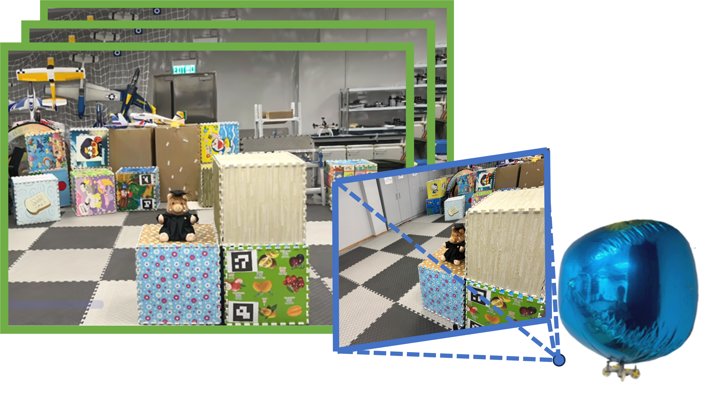
Figure 1: NuRF achieves monocular localization on images generated from radiance fields. The image within the blue box is observed by our blimp robot, while the image in the green box is a reference image rendered from radiance fields..

In recent years, the neural radiance field (NeRF) has emerged as a novel implicit representation [8], enabling the generation of high-quality, dense photographic images without the need for intricate feature extraction and alignment. This has led to the exploration of using NeRF-based map representations in pose estimation tasks. Maggio et al. [9] proposed to use particle filter as a back-end estimator for pose estimation from radiance field-based maps. Our previous work by Lin et al. [7] utilized similar techniques, incorporating VPR for pose estimation. However, current methods primarily rely on pixel-level differences for estimating robot positions, disregarding the valuable semantic and feature information present in the rendered images. This limitation results in slow convergence, particularly in global localization tasks.

To address these limitations, we design a nudged particle filter framework in radiance fields (NuRF), which achieves robot visual localization only using NeRF as map. NuRF incorporates the nudged technique and adaptive image resolution, thus enhancing global localization and pose tracking performances. Specifically, it generates a diverse set of 2D submanifold images on the special Euclidean group (SE(3)) and vectorizes them using a place recognition network. This process creates a comprehensive vector database that encapsulates the rich information present in the radiance fields. This vector database forms the foundation of our particle filter, representing the posterior probability density of the robot’s pose through particle distributions and weights. By utilizing this database, NuRF is able to estimate and track the robot pose more robustly and accurately.

In summary, our primary contributions are threefold:

• We set anchor poses for visual place recognition, improving the convergence of particle filters by nudging.

• We design an adaptive scheme that switches between global localization and position tracking, thus achieving robust and efficient indoor visual localization.

• All experiments are conducted with our blimp robot in the real world, with ablated tests.

The rest of our paper is organized as follows: Section II introduces the related work on radiance field, visual place recognition, and nudged particle filter; Section III presents the problem formulation and system overview. We detail the proposed method in Section IV and demonstrate its effectiveness with real-world experiments in Section V. The conclusions and future studies are summarized in Section VI.

II Related Work

II-A Radiance Field

A radiance field is a representation of how light is distributed in three-dimensional space, capturing the interactions between light and surfaces in the environment [10]. In the context of neural radiance fields, i.e., NeRF, it allows us to generate images from a neural model by giving any given camera pose. Hence, the neural radiance field can be seen as a low-dimensional sub-manifold that encompasses all the rendered images of the scene in a high-dimensional pixel space. In recent years, NeRF is a new wave for robotic applications, as summarized in the survey paper [11].

Loc-NeRF by Maggio et al. [9] introduced a Monte Carlo localization method for estimating the posterior probability of individual camera poses in a given space by rendering multiple random images within a radiance field. These rendered images are then compared to the target image in pixel space, evaluating the pixel-space distances. The recent advancement in explicit neural radiance field Gaussian splatting [12] has achieved a rendering rate of 160 frames per second (fps) per image while requiring less than 500MB of storage [13]. Moreover, this technology can be implemented using handheld devices such as smartphones [14]. In the 3DGS-ReLoc by Jiang et al. [15], Gaussian splatting representation was utilized for visual re-localization in urban scenarios, following a coarse-to-fine manner for global localization. Specifically, the camera was first located by similarity comparisons, and then refined by the PnP technique.

This study is inspired by the Loc-NeRF [9]. Their work demonstrated that robot localization can be performed with a radiance field-based map. However, it is worth noting that the evaluation of the algorithm’s localization performance was limited to a confined space. Even using simulated annealing for acceleration, it still requires over 400 hours to achieve a position estimation error of 0.5 $m$ within a 4 $m^{2}$ room. This indicates that the proposed method may not be practically feasible for engineering implementation.

II-B Visual Place Recognition

Visual place recognition (VPR) is a fundamental problem in robotics and computer vision [3], aiming to provide a coarse pose estimation by retrieving geo-referenced frames in close proximity. Modern learning-based VPR solutions, such as AnyLoc [16], offer comprehensive and accurate frame retrieval due to their robust representation of both images and maps. However, VPR achieves localization by considering the reference pose approximating the query pose. This inherent approximation limits the localization accuracy, especially when there is a significant deviation between the current pose and the queried poses in the database. Consequently, VPR is typically employed as a coarse or initial step in high-precision localization systems [17], which is also analyzed in the survey paper for global LiDAR localization [2]. On the other hand, constructing a database of landmark anchors for reference purposes can be a time-consuming and labor-intensive process. It involves collecting a reference image database from the robot’s onboard camera and odometer data as it navigates through the environment.

II-C Nudged Particle Filter

Nudging refers to a sampling approach in particle filtering that guides particles towards regions of high expected likelihood [18]. This technique is particularly effective when the posterior probabilities concentrate in relatively small areas of the state space, making it well-suited for high-resolution observation models, such as images. In our previous work conducted by Lin et al. [7], we conducted experiments demonstrating that the utilization of nudging particles enabled accurate tracking of a robot’s pose, even in cases where the initial distribution was incorrect and had low variance. However, we did not achieve successful global localization using the nudged particle filter in that particular study.

III Problem Formulation and System Overview

Mathematically, both implicit and explicit radiance fields can be represented as a pair, denoted as $[\mathcal{G},L]$. The term $\mathcal{G}$ represents a 3D scene in the world frame, and $L$ is the rendering function that takes $\mathcal{G}$ and a pair of camera parameters $[K,T]$ as inputs and produces the rendered image $I_{\mathcal{G}}$. The rendering function $L$ can be formulated as:

$$I_{\mathcal{G}}=L(\mathcal{G},K,T)$$ (1)

in which camera parameter $K$ is the intrinsic matrix that encodes the field of view and the resolution of the rendered image, and the extrinsic matrix $T\in$ SE(3) represents the 6-DoF pose of the camera regarding the world frame. For convenience, let the pose of a camera-mounted robot at time $\tau$ be the same as the extrinsic matrix of the camera $T_{\tau}$. From time $\tau-1$ to $\tau$, the robot pose is integrated by relative transformations $H_{\tau}\in$ SE(3), described as follows:

$$T_{\tau}=T_{\tau-1}H_{\tau}=\begin{bmatrix}\boldsymbol{R}_{\tau-1}\boldsymbol{V}_{\tau}&\boldsymbol{R}_{\tau-1}\boldsymbol{u}_{\tau}+\boldsymbol{t}_{\tau-1}\\ \boldsymbol{0}^{T}&1\end{bmatrix}$$ (2)

in which $\boldsymbol{t},\boldsymbol{u}\in\mathbb{R}^{3}$ are the translation vectors and $\boldsymbol{R},\boldsymbol{V}\in\mathbb{R}^{3\times 3}$ are rotation matrices. For two consecutive poses, we assume the sensors equipped on the robot can capture two images $I_{\tau-1}$, $I_{\tau}$ and the motion $\hat{H}_{\tau}$. Note that the motion model is perturbed by noise $\boldsymbol{\epsilon}\sim\mathcal{N}(0,\Sigma)\in\mathbb{R}^{3}$ and $\boldsymbol{\varepsilon}\sim\boldsymbol{U}[-a,a]\in\mathbb{R}^{3}$. The relative transformation is therefore given by:

$$\hat{\boldsymbol{u}}_{\tau}=\boldsymbol{u}_{\tau}+\boldsymbol{\epsilon}$$ (3)

$$\hat{\boldsymbol{V}}_{\tau}=f_{\boldsymbol{R}}(\boldsymbol{\varepsilon})\boldsymbol{V}_{\tau}$$

where $f_{\boldsymbol{R}}$ converts the sampled Euler angle to a rotation matrix. Then, the posterior probability density function of the robot pose $T_{\tau}$ can be written as:

$$p(T_{\tau}|I_{1:\tau},\hat{H}_{2:\tau})=\frac{p(I_{1:\tau}|\hat{H}_{2:\tau},T_{\tau})p(\hat{H}_{2:\tau},T_{\tau})}{p(I_{1:\tau},\hat{H}_{2:\tau})}$$ (4)

Then, we can formulate the visual-based global localization problem as Problem III.1.

Problem III.1

Given a sequence of RGB images $\boldsymbol{I}=[I_{1},I_{2},\dots,I_{\tau}]$ and a motion model $\boldsymbol{\hat{H}}=[\hat{H}2,\hat{H}3,\dots,\hat{H}{\tau}]$, the task is to approximate the posterior distribution of the robot pose $T{\tau}$ as delineated in equation (4), and to achieve the maximum likelihood estimation of the robot pose, denoted as $T^{*}_{\tau}$.

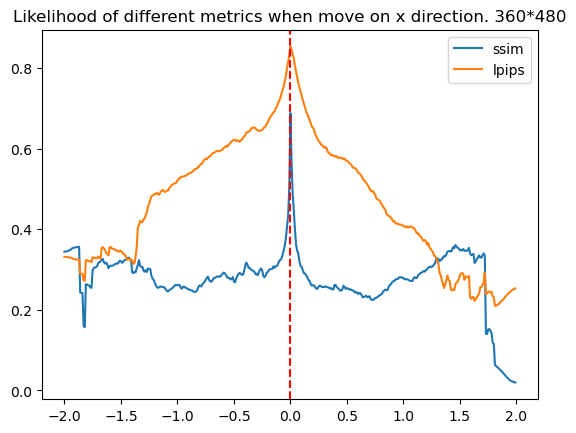
(a) X direction

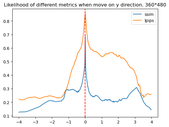
(b) Y direction

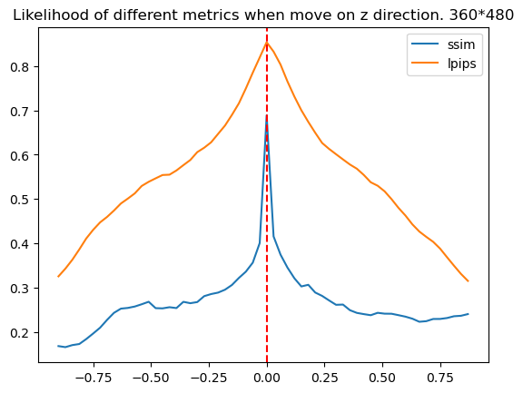
(c) Z direction

Figure 2: We assess the similarity between a query image and images rendered in the same orientation but shifted along the X/Y/Z axis using pixel-wise similarity (SSIM) and feature-wise similarity (LPIPS).

Let $\varXi_{\tau}=\{\zeta_{\tau,i}\}^{N}_{i=1}$ be the set of particles at time $\tau$, where each particle $\zeta_{\tau,i}=[w_{\tau,i},T_{\tau,i}]$ with weight $w_{\tau,i}$ and pose $T_{\tau,i}$. Consequently, the posterior probability density function (4) can be approximated as follows:

$$f(z;\varXi_{\tau})=\eta\sum_{i=1}^{N}w_{\tau,i}\delta(z-T_{\tau,i})$$ (5)

in which $\delta$ is the Dirac delta function, and $\eta$ is a normalisation constant; if $T_{\tau,i}$ is a sample point in (4) and $w_{\tau,i}$ presents the likelihood that the camera captured image $I_{\tau}$ at $T_{\tau,i}$ after motions $\hat{H}_{2:\tau}$ as:

$$w_{\tau,i}=p(I_{\tau}|\hat{H}_{2:\tau},T_{\tau})=\frac{p(I_{1:\tau}|\hat{H}_{2:\tau},T_{\tau})}{p(I_{1:\tau-1}|\hat{H}_{2:\tau},T_{\tau})}$$ (6)

It’s very difficult to calculate (6) directly. But, with the radiance field representation, we could approximate (6) using the similarity between the rendered images and the observed image at $T_{\tau,i}$. The most intuitive method to calculate the similarity between two images is calculating the pixel-wised distances between those images. The structural similarity index measure (SSIM) [19] is a typical pixel-wised image similarity function. With SSIM, the distance between image $x$ and $y$ can be calculate as:

$$\text{Distance}(x,y) =1-\text{SSIM}(x,y)$$ (7)

$$=1-\frac{(2\mu_{x}\mu_{y}+c_{1})(2\sigma_{xy}+c_{2})}{(\mu_{x}^{2}+\mu_{y}^{2}+c_{1})(\sigma_{x}^{2}+\sigma_{y}^{2}+c_{2})}$$

in which $\mu$ and $\sigma$ represent the mean and standard deviation of each image, respectively. Another kind of method involves learning techniques that transform the image into a learned feature space and subsequently utilize the distances within this feature space to estimate the similarity. A typical approach is learned perceptual image patch similarity (LPIPS)[20]:

$$\text{Distance}(x,y) =\text{LPIPS}(x,y)$$ (8)

$$=\sum_{l}^{L}\frac{\sum_{h,w}||w_{l}\odot(\hat{x}^{l}_{hw}-\hat{y}^{l}_{h}w)||^{2}_{2}}{H_{l}W_{l}}$$

in which $\hat{x}^{l}$ and $\hat{y}^{l}$ represent the feature maps of the images at a particular feature layer, and $w_{l}$ denotes the corresponding layer weight.

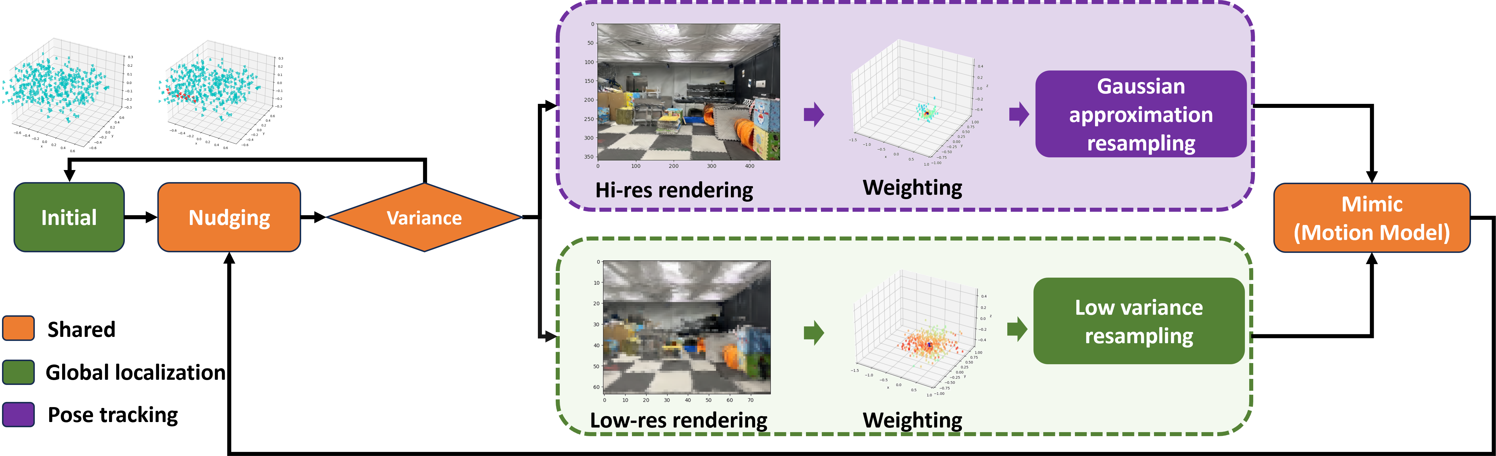
Figure 3: The pipeline of our designed NuRF framework. We first use radiance fields to generate images on anchor poses, store these images in a database, and vectorize them for retrieval. Then, a particle filter is built for robot localization in radiance fields. The nudging step uses retrieved results (from VPR) to guide the particles toward more confident states. The measurement model updates particle weights based on images that are observed and rendered by particles. The motion model adjusts particles according to robot motion. Our adaptive workflow enables switching between global localization and pose tracking to address the robot kidnapping problem.

Figure 2 shows that the linear correlation between image similarity and robot pose is more prominent when utilizing the feature-wised approach [21]. This attribute makes it easier to employ the feature-wised similarity as the key factor to approximate the term in (6). However, although it is more accurate to use the feature-wise similarity function to weight particles, projecting the image rendered by each particle into the feature space needs large computing resources. Therefore, a pixel-based similarity function is required if a real-time particle filter is needed. This leads to Problem 9.

Problem III.2

Given two particle sets $\varXi^{1}$ and $\varXi^{2}$. Known that $T^{1}\equiv T^{2}$, and $w^{1}$ and $w^{2}$ are calculated by (7) and (8) respectively. Add some extra particles into $\varXi^{1}$ to get $\varXi^{1+}$. And make $\varXi^{1+}$ satisfied:

$$\varXi^{1+}=\arg\min_{\varXi^{1+}}\parallel 1-\frac{f(z;\varXi^{2})}{f(z;\varXi^{1+})}\parallel$$ (9)

The solution to Problem 9 holds the key to effectively addressing Problem III.1 for practical deployment. Furthermore, in practice, another classic problem in robot localization is the kidnapping problem, which can be described as Problem III.3.

Problem III.3

Move the robot to a new location and observe a new image $I_{\tau+1}$, but incorrect motion information is provided. Detect this motion in limited time steps.

To address the outlined problems, we introduce the NuRF framework as depicted in Figure 3. This framework integrates anchor points in close proximity to the target image $I_{\tau}$ within the feature space during the resampling phase. By implementing this strategy, both Problem 9 and Problem III.1 are effectively addressed for real-world deployment. Additionally, the utilization of nudging particles facilitates the monitoring of particle dispersion, i.e., the variance of particles, which is used to switch the global localization and poser tracking in the radiance fields. We will detail the NuRF modules in the following section.

IV Methodology

IV-A Anchor Setting in Radiance Fields

Pixel-wised similarity is sensitive to translational movement, as shown in Figure 2. Even if the orientation error is $0$, only images rendered in a very small spatial neighborhood of the target image location can obtain a high similarity response. In global localization, when the number of particles is limited, the probability of randomly generated particles falling into this neighborhood is also very small, and the particle filter might fail to converge to the ground truth pose.

In order to overcome these problems and build an efficient NuRF (Problem III.1), we introduce the VPR on anchor poses. As shown in Figure 4, VPR technology requires a set of anchor points in the space and stores the images generated at these anchor points. Specifically, we detail the anchor setting in Algorithm 1, the process initiates by sampling a set of 3-DoF anchors, denoted as $s=(x,y,\omega)$, from a 2D sub-manifold of SE(3). Subsequently, each anchor $s$ is converted into a 6-DoF pose $\xi=(\eta_{1},\eta_{2})$ by incorporating zero values for the z-axis, pitch, and roll angles. This conversion employs the exponential map for $\xi$ to SE(3), as follows:

$$\exp{(\xi^{\wedge})}=\sum_{n=0}^{\infty}\frac{1}{n!}(\xi^{\wedge})^{n}=\begin{bmatrix}\boldsymbol{R}&\boldsymbol{t}\\ \boldsymbol{0}&1\end{bmatrix}$$ (10)

Following this, the rendered image $I$ is embedded into a feature space $\boldsymbol{F}$ using a pre-trained embedding function [22]. Both the image feature $\boldsymbol{F}$ and the pose $T$ are subsequently stored in a database $\boldsymbol{D}$.

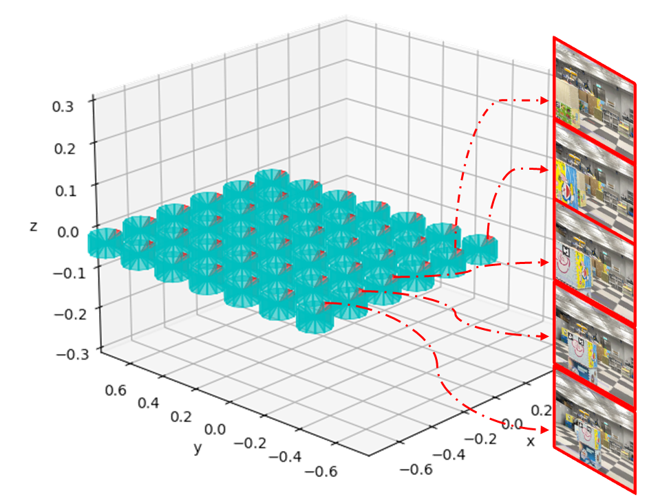
Figure 4: We display 504 anchor poses in 2D sub-manifold $S$, along with images rendered at these specific anchors for visualization.

1

Input : $\mathcal{G},L,K,N,S$

Output : $\boldsymbol{D}$

2

3$\boldsymbol{T}\leftarrow\emptyset$;

4 $\boldsymbol{F}\leftarrow\emptyset$;

5 $\boldsymbol{S}\leftarrow[(x_{1},y_{1},\omega_{1}),\dots,(x_{N},y_{N},\omega_{N})]$;

6

7for $s\in\boldsymbol{S}$ do

8       $\xi\leftarrow[s[1],s[2],0,s[3],0,0]$;

       $T\leftarrow\exp{(\xi^{\wedge})}$ ;

        // Equation (10)

       $I\leftarrow L(\mathcal{G},K,T)$ ;

        // Equation (1)

9       $\boldsymbol{F}\leftarrow\boldsymbol{F}\cup$ Embedding($I$);

10       $\boldsymbol{T}\leftarrow\boldsymbol{T}\cup T$;

11      

12 end for

13

14$\boldsymbol{D}\leftarrow\{\boldsymbol{F}:\boldsymbol{T}\}$;

15

16return $\boldsymbol{D}$;

17

Algorithm 1 Anchor Setting in Radiance Fields

IV-B Nudging by Visual Place Recognition

After generating the VPR anchors, we need to incorporate the reference information provided by the VPR results into the pixel-wised weighting particle filter to solve Problem 9. We adopt the definition of the nudging step provided by Akyildiz[18], illustrated in Definition IV.1. In this definition, $x_{\tau}\in\mathsf{X}$ represents the system state at time $\tau$, and $y_{\tau}$ denotes the observations at time $\tau$. The state after the nudging step is denoted as $x^{+}$.

Definition IV.1

A nudging operator $\alpha_{\tau}^{y_{\tau}}:\mathsf{X}\rightarrow\mathsf{X}$ associated with the likelihood function $g_{\tau}(x)$ is a map such that if $x^{+}=\alpha_{\tau}^{y_{\tau}}(x)$, then $g_{\tau}(x^{+})\geq g_{\tau}(x)$.

Intuitively, the nudging step adapts the generation of particles in a manner that is not compensated by the importance of weights but enhances the likelihood of accurate estimation. To achieve this, we have developed a novel technique termed VPR nudging.

Figure 5 demonstrates the VPR nudging step, as illustrated in Definition IV.1. The algorithm inputs include the reference image database $\boldsymbol{D}$ at anchors, the observed image $I$, the number of nudging particles $M$, the radiance field $[\mathcal{G},L]$, and the low-resolution camera intrinsic $K^{-}$. The objective is to identify the top $M$ images in the database $D$ that are most similar to $I$ and to render low-resolution images $I_{m}$ at each corresponding pose $T_{m}$. If the weight of nudged particles $w_{m}$ exceeds the current average weight $\bar{w}$, the pose $T_{m}$ is incorporated into the nudging particle set $\varXi^{+}$.

The VPR nudging step modifies the stochastic generation of particles in a manner that is not offset by the importance weights. This strategic alteration enables the integration of valuable feature information without necessitating computationally intensive embedding operations on every image rendered by particles. This approach enhances both the accuracy and efficiency of the global localization.

IV-C Adaptive Scheme in NuRF

Figure 5: Particles are nudged by retrieving and utilizing images corresponding to anchors.

We introduce an adaptive scheme within the particle filter framework to switch the global localization and pose tracking. Initially, in global localization, we lower the resolution of both the input and rendered images. This reduces localization accuracy slightly but expands the area where high similarity responses are detected, lessening sensitivity to small movements. As the process iterates and the particles begin to converge, we maintain the original input image quality and enhance the resolution of the rendered images to improve pose tracking accuracy. This adaptive strategy dynamically adjusts the resolution based on the discrepancy between nudged and original particles. This approach effectively addresses the issues of particle deficiency in global localization and aids in automatic recovery from kidnapping scenarios (Problem III.3).

Specifically, after each nudging step, we calculate the weighted variance of the current particles. This variance indicates how close the particle filter is to converging and reflects the diversity of particle distribution. It directly influences how we adjust the resolution in the image rendering process to optimize accuracy and performance. The weight variance is defined as follows:

$$\bar{T} =\frac{1}{N}\sum_{i=1}^{N}w_{i}T_{i}$$ (11)

$$\Sigma_{T} =\frac{1}{N}\frac{\sum_{i=1}^{N}w_{i}(T_{i}-\bar{T})(T_{i}-\bar{T})^{T}}{\sum_{i=1}^{N}w_{i}}$$ (12)

in which $\Sigma_{T}$ is a metric for assessing the convergence of the particle filter. When the weighted variance of the particles drops below a set threshold $\lambda$, the system shifts to a higher resolution setting ($K^{+}$), improving the accuracy of pose estimation. If the variance exceeds this threshold, the algorithm switches to a lower resolution setting ($K^{-}$), reducing computational load and increasing the efficiency of robot localization. The strategy is described as:

$$K=\left\{\begin{array}[]{r c l}K^{+}&&{\Sigma_{T}\leq\lambda}\\ K^{-}&&{\Sigma_{T}>\lambda}\\ \end{array}\right.$$ (13)

The system pipeline, as depicted in Figure 3, seamlessly integrates VPR nudging and adaptive resolution rendering techniques. Particle adjustments span extensive areas using low-resolution rendering for the global localization phase at a lower resolution ($K=K^{-}$). The resampling weights for this phase are calculated as follows:

$$w_{\tau,j}=\frac{\text{SSIM}(I_{\tau},L(\mathcal{G},K^{-},T_{\tau,j}))}{\sum_{i=1}^{N}\text{SSIM}(I_{\tau},L(\mathcal{G},K^{-},T_{\tau,i}))}$$ (14)

Conversely, during the local pose tracking phase at a higher resolution ($K=K^{+}$), the particle updates are refined in more confined areas using high-resolution rendering. The resampling weights in this phase are determined by:

$$w_{\tau,j}=\mathcal{N}(T_{\tau,j};\mu_{\tau},\Sigma_{\tau})$$ (15)

where $\mu_{\tau}$ and $\Sigma_{\tau}$ represent the weighted mean and variance, respectively, detailed in Equations (11) and (12). The Gaussian approximate resampling technique, often used in this phase, is particularly suited for environments expected to exhibit a single-peak distribution. This method is crucial in high-resolution settings, where even minor distortions such as rotations and translations can significantly impact particle convergence. The strategies for both global localization and local pose tracking, thoroughly described in Algorithm 2 and Algorithm 3, ensure robust performance across varying environmental complexities.

1

Input : $\varXi_{\tau-1},I_{\tau},\mathcal{G},L,D,M$

2

3for $\zeta_{\tau-1,i}\in\varXi_{\tau-1}$ do

       $T_{\tau,i}\leftarrow T_{\tau-1}H_{\tau}$ ;

        // Equation (2)

       $\hat{I}_{\tau,i}\leftarrow L(G,K^{-},T_{\tau,i})$ ;

        // Equation (1)

       $w_{\tau,i}\leftarrow$ SSIM($I_{\tau},\hat{I}_{\tau,i}$) ;

        // Equation (14)

4      

5 end for

6

$\varXi^{+}_{\tau}\leftarrow\alpha(D,I_{\tau},M,\mathcal{G},L,K^{-})$ ;

  // Nudging

7

8$\varXi^{\dagger}_{\tau}\leftarrow\emptyset$

9for $\zeta_{\tau,i}\in\varXi_{\tau}$ do

10       $\zeta^{\dagger}_{\tau,i}\leftarrow$ resampling($f(z;\varXi^{+})$)

11      $\varXi^{\dagger}_{\tau,i}\leftarrow\zeta^{\dagger}_{\tau,i}$

12 end for

13

14return $\varXi^{\dagger}_{\tau}$;

15

Algorithm 2 Global Localization

1

Input : $\varXi_{\tau-1},I_{\tau},\mathcal{G},L,D,M$

2

3for $\zeta_{\tau-1,i}\in\varXi_{\tau-1}$ do

       $T_{\tau,i}\leftarrow T_{\tau-1}H_{\tau}$ ;

        // Equation (2)

       $\hat{I}_{\tau,i}\leftarrow L(G,K^{+},T_{\tau,i})$ ;

        // Equation (1)

       $w_{\tau,i}\leftarrow$ SSIM($I_{\tau},\hat{I}_{\tau,i}$) ;

        // Equation (14)

4      

5 end for

6

$\varXi^{+}_{\tau}\leftarrow\alpha(D,I_{\tau},M,\mathcal{G},L,K^{+})$ ;

  // Nudging

7

$\mu_{\tau}\leftarrow$ E($\varXi^{+}_{\tau}$) ;

  // Equation (11)

8

$\Sigma_{\tau}\leftarrow$ Var($\varXi^{+}_{\tau}$) ;

  // Equation (12)

9

10$\varXi^{\dagger}_{\tau}\leftarrow\emptyset$

11for $\zeta_{\tau,i}\in\varXi_{\tau}$ do

12       $\zeta^{\dagger}_{\tau,i}\leftarrow$ resampling($\mathcal{N}(\mu_{\tau},\Sigma_{\tau})$)

13      $\varXi^{\dagger}_{\tau,i}\leftarrow\zeta^{\dagger}_{\tau,i}$

14 end for

15

16return $\varXi^{\dagger}_{\tau}$;

17

Algorithm 3 Pose Tracking

V Experiments and Evaluation

We validate the proposed NuRF in a motion capture room, which is a typical indoor environment with cluttered objects. The experiments are designed to assess the performance in terms of global localization and pose tracking, i.e., the convergence from scratch and local tracking accuracy. Additionally, within the NuRF framework, we conduct a thorough comparison of three widely used image similarity functions: SSIM, complex wavelet-SSIM (CW-SSIM)[23], and LPIPS. These functions calculate image similarity in different spaces and allow us to assess the impact of the nudging step on the approximation of the posterior distribution in the particle filter. All the experiments are conducted on a blimp robot [24].

V-A Experimental Setup

V-A1 Radiance Field in Indoor Environments

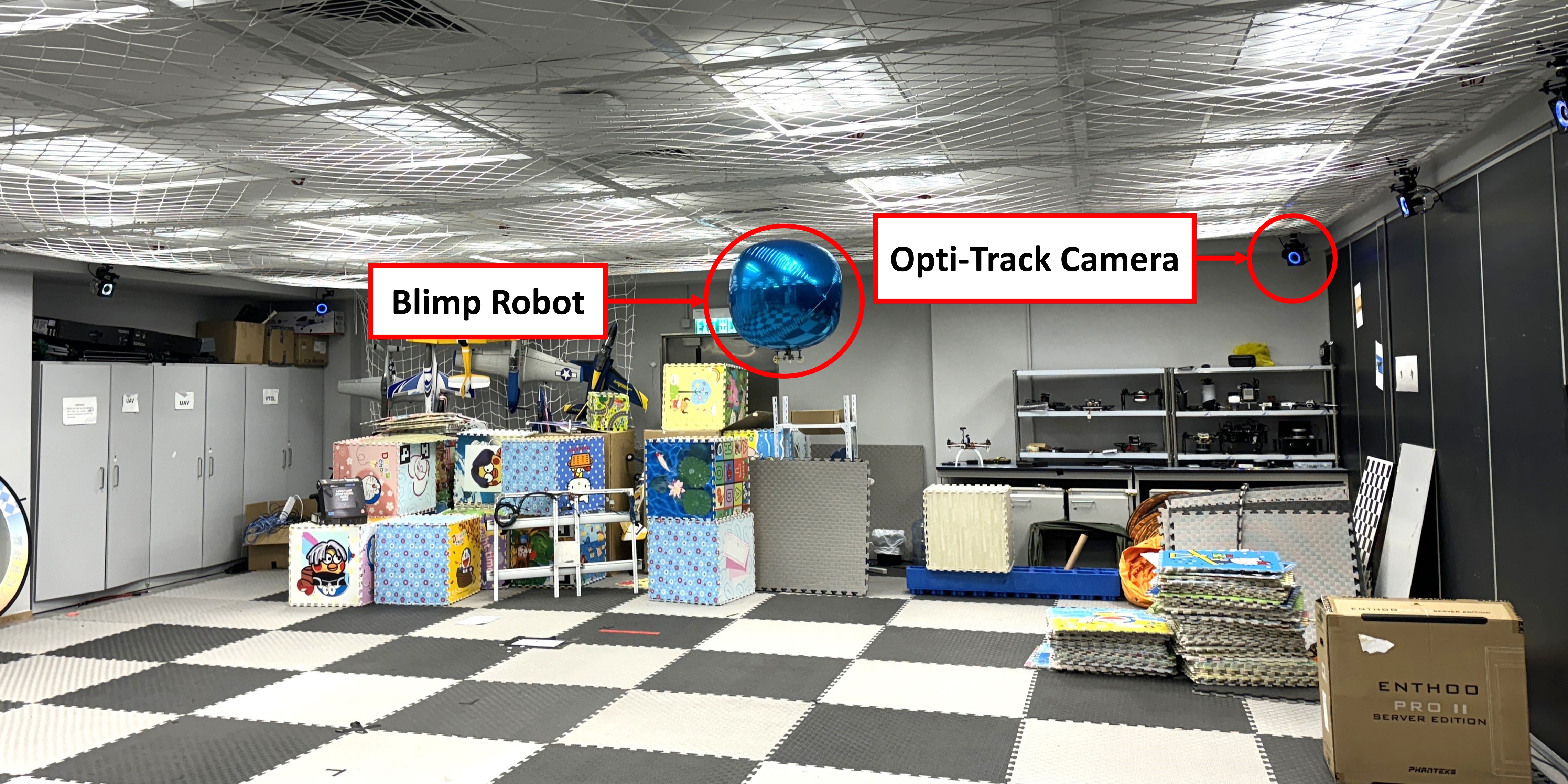
(a) Experimental setup

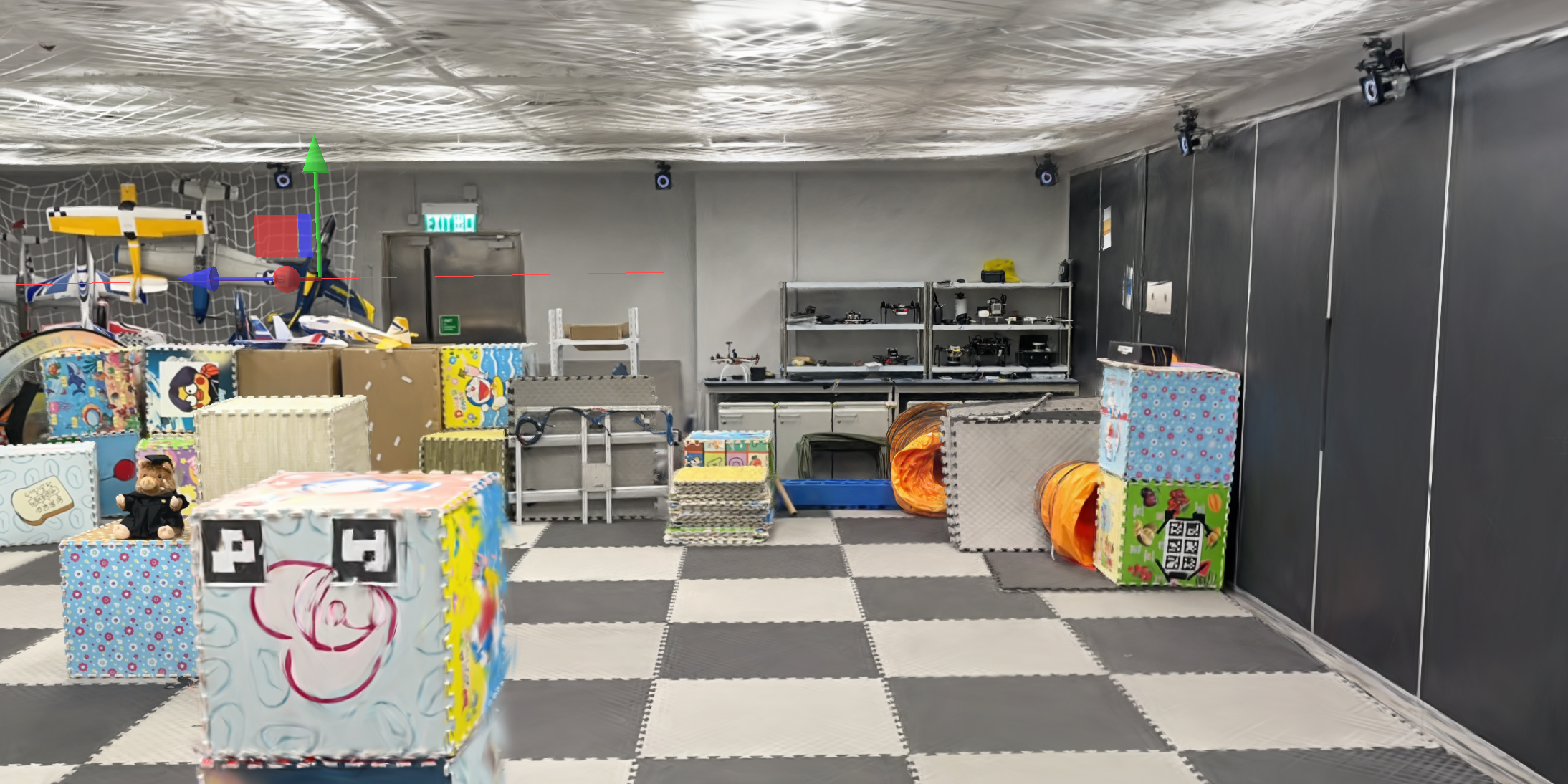
(b) Rendered image

Figure 6: (a) A Blimp robot in our motion capture room for experimental evaluation. (b) A rendered image in the motion capture room that closely mimics the real-world scenario.

Our method relies on a pre-trained 3D radiance field as a pre-built map for robot localization. We directly utilize the 3DGS [12], a real-time radiance field rendering technique known for its state-of-the-art performance. The input of the 3DGS is a trajectory consisting of continuous camera poses and corresponding images at each pose, which can be easily obtained on our blimp robot.

Our blimp robot is equipped with one camera for monocular localization. The robot was operated remotely within a 4-meter by 5-meter fly arena, as shown in Figure 6(a). A motion capture system is installed. to obtain the ground truth poses. To generate the 3DGS of the room, 534 images with a $1440\times 1920$ resolution are captured, and the rendered image is shown in Figure 6(b).

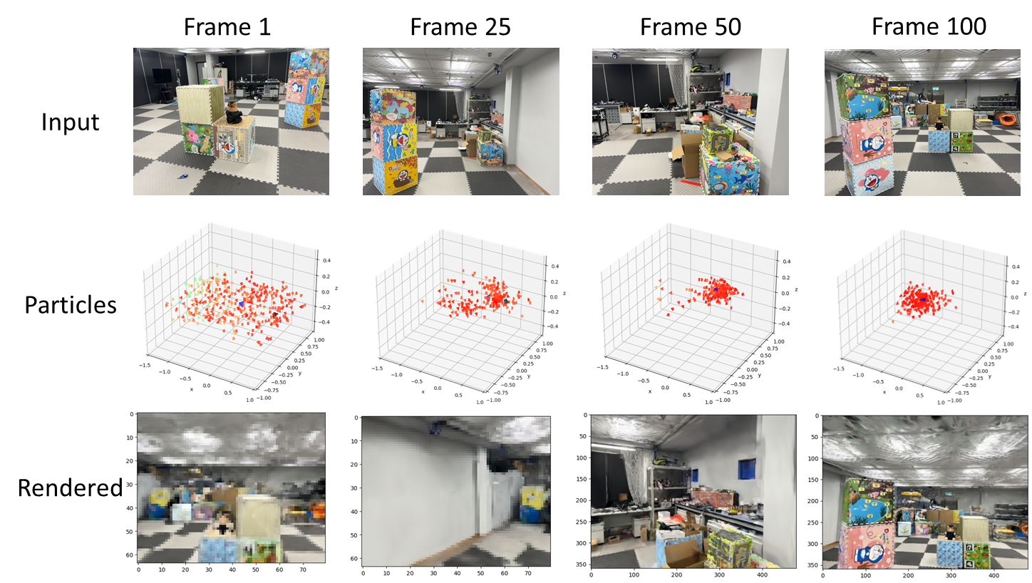
Figure 7: A case study for global visual localization in radiance fields. Top: Sequential observed images of the robot at frame 1, frame 25, frame 50, and frame 100. Middle: Particle filter states for each frame are shown. The larger blue pyramid indicates the estimated pose, while the black pyramid represents the ground truth pose. Smaller pyramids symbolize the particles, colored according to the visible spectrum, with red indicating the highest similarity and purple the lowest. Bottom: Rendered images at the estimated pose are shown, with the rendering resolution adapting from low to high based on the variance of particles.

V-A2 Image Database for Retrieval

In Section IV, an additional assumption is made that the radiance field could provide valuable visual place retrieval information to guide the particle behavior. Once the 3D radiance field is constructed, we then generate images from any desired pose within the model. We establish anchor points, denoted as $a=[x,y,\omega]$, uniformly on a two-dimensional sub-manifold of SE(3). Images are rendered from these anchor points and encoded into vectors using the Vision Transformer technique. The resulting vector representations, derived from the anchor point images, are then stored as vectors for the next steps.

V-A3 Implementation Details

The experiments are conducted with Pytorch-based implementation. The computing hardware comprises an Intel CPU i7-13700KF and a GeForce RTX4080 GPU. The input image size was set to $680\times 800$, with a render resolution of $64\times 80$ for global localization and a render resolution of $680\times 800$ for pose tracking. The thresholds for global localization and pose tracking switching were set to $\lambda^{+}=5$, while the threshold for kidnapping detection was set to $\lambda^{-}=15$.

V-B Global Visual Localization

To evaluate the NuRF method’s performance in global localization, we conducted experiments with 20 randomly chosen sets of image sequences. Each set contained 100 frames depicting continuous motion.

In Figure 7, the first column illustrates the utilization of 400 particles. The initial positions of these particles were obtained by uniformly perturbing the dimensions of the room, which has a height of $1.8m$, a length of $5m$, and a width of $4m$. For orientation, the yaw angles were uniformly initialized within the range of $[-180^{\circ},180^{\circ}]$, while the pitch and roll angles for all particles were set to $0^{\circ}$. Once the experiment begins, the motion model provides a 6-DoF (six degrees of freedom) motion matrix to update the pose of the particle swarm (depicted in the second to fourth columns of Figure 7). The resampling process also occurs in the 6-DoF space, meaning that the algorithm optimizes the particles in a complete 6-DoF state and performs only one update per image.

Furthermore, we conduct experiments involving three different similarity functions: SSIM, CW-SSIM, and LPIPS in Figure 8. These experiments demonstrate that the NuRF algorithm can enable the pixel-wise difference function to achieve a similar level of localization mean squared error (MSE) median as the feature-based difference functions. The results of these experiments are presented in Figure 9, which showcases 20 trials with the designed NuRF.

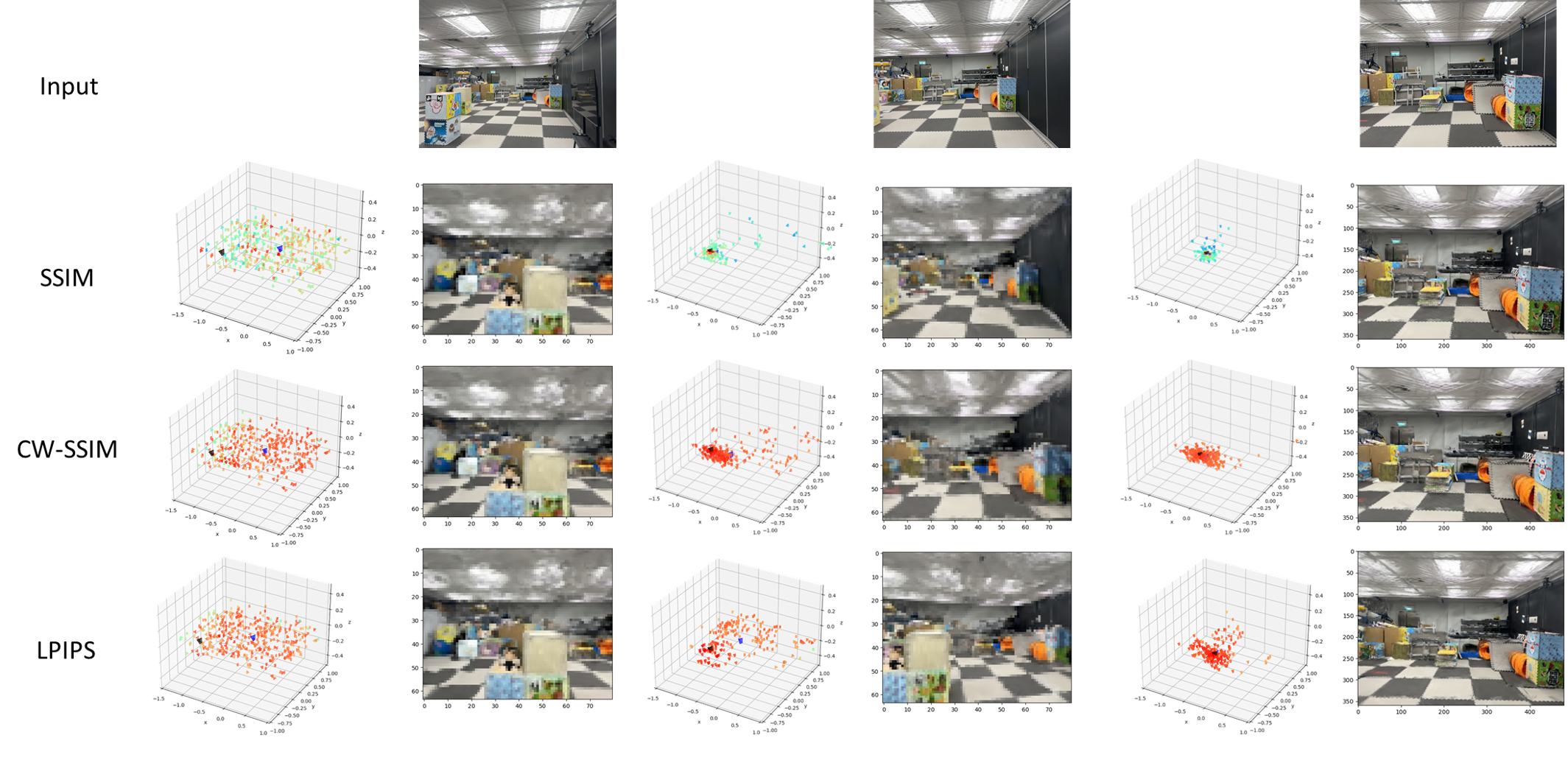
Figure 8: Global visual localization with different similarity evaluation functions in sub-manifold. First Row: From left to right are the observed images of the robot in frame 1, frame 25, and frame 50, respectively. Second to Fourth Row: The global localization performance of NuRF when using different similarity evaluation functions.

Figure 9(a) showcases the accuracy of global localization and the convergence efficiency achieved with different similarity functions. The results demonstrate the exceptional performance of the NuRF method in the global localization task, even using the pixel-wised similarity metric to calculate the importance factor of the particles. When considering both running time and localization accuracy, the combined comparison in Figure 9(b) demonstrates that the pixel-wise similarity function outperforms the feature-wise similarity function in terms of median running cost. This outcome highlights the capability of the NuRF framework to address the limitations associated with using the pixel-wise similarity function as the likelihood function, thereby achieving a more efficient and effective localization process.

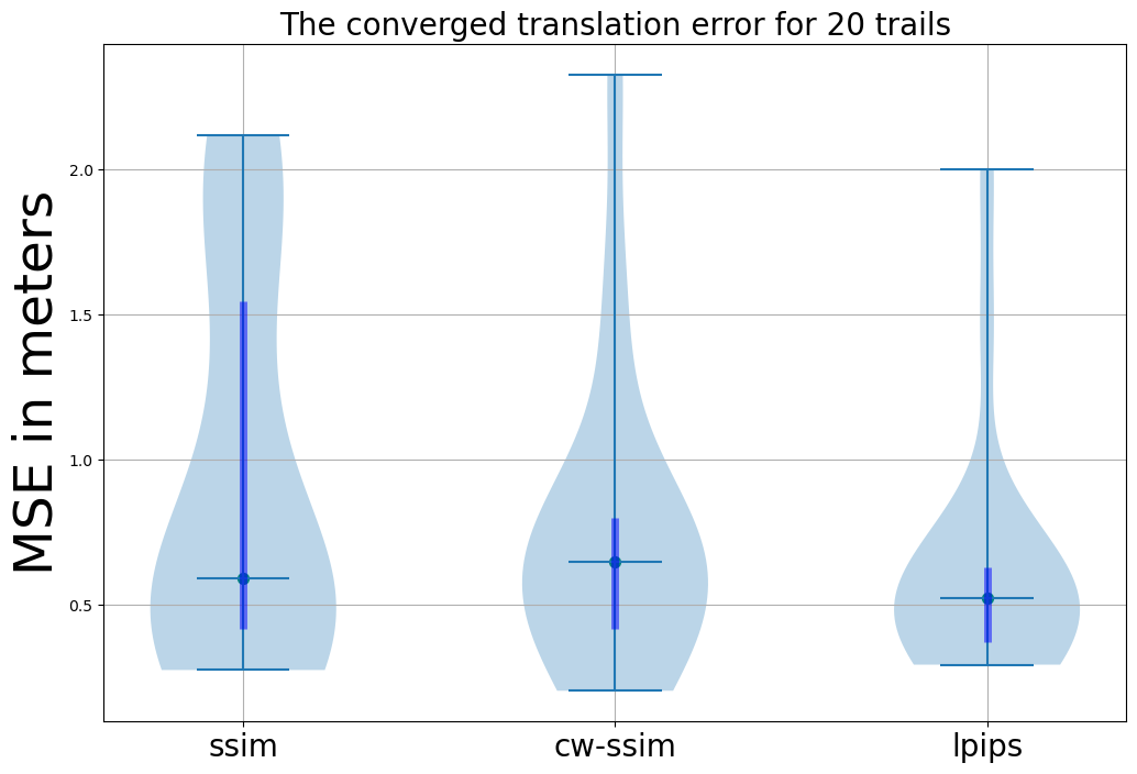
(a) Translational Mean Square Error

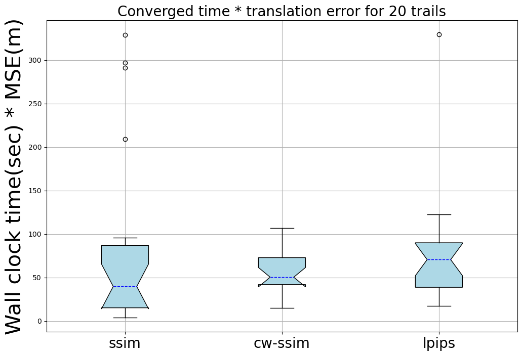
(b) Convergence time $\times$ Translational Mean Square Error

Figure 9: (a) The performance during the global localization task is depicted through violin plots derived from 20 independent trials. (b) We also show the product of convergence time and mean square translation error across all configurations.

V-C Pose Tracking in Radiance Fields

In this section, we evaluate the performance of the NuRF method in a pose tracking task using images captured from a blimp. We initiate the tracking process with the pose estimation obtained in Section V-B. We employ $200$ particles for the pose tracking task and initialize their positions by sampling from a normal distribution centered around the estimated position. The variances for the position dimensions are set to $[0.2,0.2,0.1]$ respectively. Similarly, we sample the yaw, pitch, and roll angles from normal distributions centered around the estimated rotation. The variances for the angles are set to $[5,1,1]$ respectively. Figure 10 illustrates the tracking process, where only one update is performed per image.

Figure 10: A case study of pose tracking. Top: observed images of the robot at key frames: frame 100, frame 110, and frame 120. Middle: The particle filter states at each frame, following the same color settings in Figure 9. Bottom: the rendered images at the estimated poses, with changes in rendering resolution based on the variance of the particles.

The demonstration presented in the first column of Figure 10 shows the re-generation of the particles around the initially estimated position when transitioning from global localization to positional tracking. In the second column of Figure 10, we observe the convergence of the particles after running the NuRF algorithm for 10 frames. In the pose tracking phase, the VPR system continues to generate particles. However, these particles are solely utilized to detect potential abduction issues and are not involved in the resampling process.

To validate the effectiveness of the NuRF, we conduct experiments on 20 randomly selected trajectories consisting of 40 frames each. These experiments aimed to demonstrate that the performance of the NuRF algorithm is not dependent on a specific similarity evaluation function. In order to further assess its adaptability, we repeated the tests using different similarity functions.

The results of orientation estimation are showing in Figure 11, the NuRF showcases its proficiency in accurately tracking yaw angles with an error margin of $15^{\circ}$ or less, irrespective of the similarity evaluation function employed (see Figure 11(a)). This emphasizes its robustness and effectiveness in precisely estimating and tracking yaw angles, regardless of the specific similarity metric utilized.

(a) Yaw Error

(b) Pitch Error

(c) Roll Error

Figure 11: (a) The average rotation error in yaw of 20 trails at each frame. The shaded area shows one standard deviation above and below the mean error. (b) The average rotation error in pitch of 20 trails at each frame. (c) The average rotation error in roll of 20 trails at each frame.

In high-resolution images, the similarity function tends to better recognize floors and ceilings in indoor scenes. The experimental results presented in Figure 11(b) show that the NuRF algorithm achieves stable tracking of the pitch angle of the camera pose within an error margin of $10^{\circ}$, regardless of the specific similarity function utilized. However, the experimental results in Figure 11(c) indicate that the tracking performance of the roll angle is influenced by the choice of similarity function. In real-time scenarios, employing feature-wise similarity functions like CW-SSIM and LPIPS for heading angle estimation entails significant computational power consumption and introduces errors in the roll direction during the resampling process. However, the use of the pixel-wise similarity function, complemented by nudging information, enables more precise and stable tracking of the robot’s pose. This suggests that the NuRF algorithm effectively compensates for and mitigates these errors, resulting in reliable roll angle tracking.

V-D Ablated Experiments

To validate the modules in NuRF, this section conducts ablated experiments on visual place recognition and explores the effect of the number of anchor points on global localization performance and the image resolution on global pose tracking performance.

TABLE I: Ablated Experiments on Anchor Number for VPR

Similarity function	Anchor number	Average translational MSE($m$)	Average convergent steps	FPS($Hz$)
	0	1.204	64.7	0.26
SSIM	504	0.951	60.1	0.23
	2502	0.642	24.2	0.21
	0	1.233	74.1	0.15
CW-SSIM	504	1.185	70.7	0.14
	2502	0.741	35.3	0.12
	0	0.984	50.3	0.07
LPIPS	504	0.865	50.9	0.07
	2502	0.517	22.5	0.07

The first ablated experiment is designed to evaluate global localization capabilities under two specific conditions: without VPR nudging (where the anchor point count was set to zero) and with attenuated VPR nudging (where the number of nudging particles was halved and the anchor point count was reduced to 504).

The results show that if there are no anchored points, i.e., no nudging step is performed, there is a noticeable decline in the accuracy. Specifically, the translational mean square error of position estimation decreases from 0.642 $m$ to 1.204 $m$ when using SSIM for visual place recognition. In terms of efficiency, the experimental results demonstrate that the nudging step leads to a slight increase in the time required for a single particle update, approximately 1 second. However, it significantly reduces the number of iteration steps needed for the convergence.

Following the convergence of global localization, the second ablation experiment assesses the impact of image resolution on pose tracking accuracy. By adjusting the resolution of rendered images, we explore its effect on the precision of the pose tracking algorithm. Figures 12, 13, and 14 present a comparison of estimation errors across different Euler angles using various rendering resolutions and perception functions. The results clearly show that using high-resolution images typically results in smaller estimation errors in two-thirds of the cases. Furthermore, a comparison with Figures 11 reveals that low-resolution images tend to perform better in the relatively simpler task of estimating the pitch angle, but they are 83% more likely to yield poorer results in the more challenging yaw and roll angle estimations. Overall, these findings strongly indicate that high-resolution images generally enhance pose tracking performance across the system.

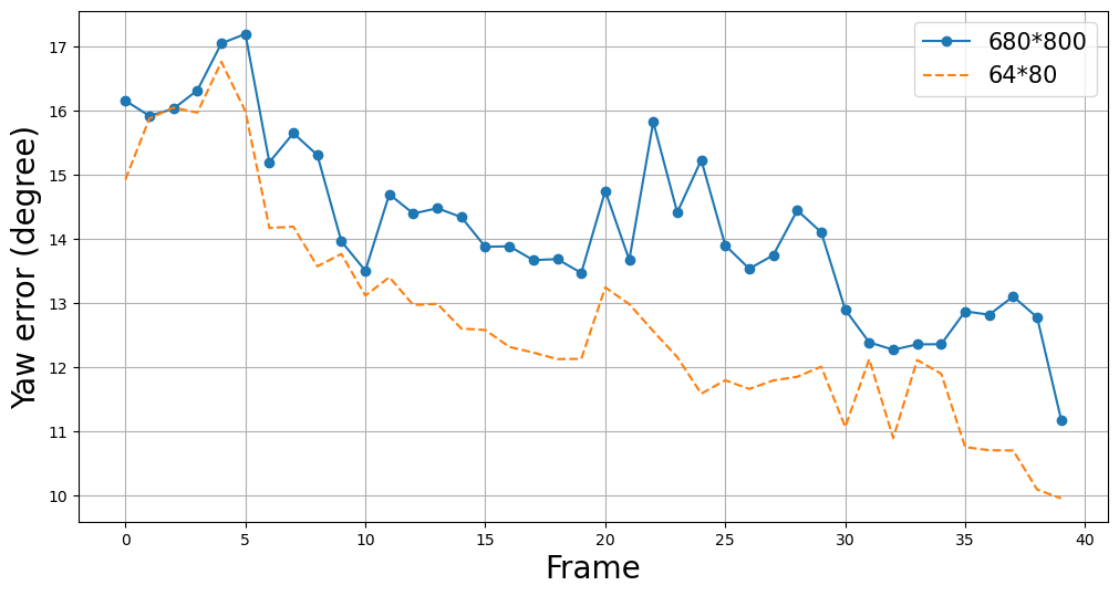
(a) SSIM

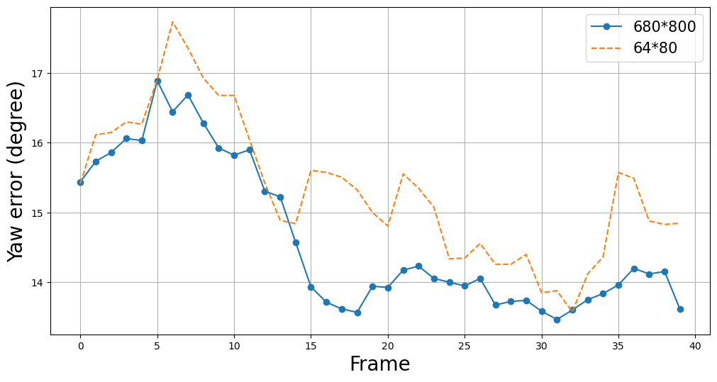
(b) CW-SSIM

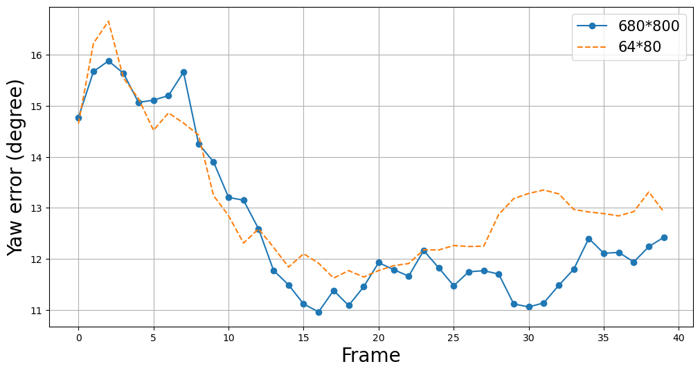
(c) LPIPS

Figure 12: (a) The comparison of average rotation error in yaw of 20 trails at each frame when using SSIM in different resolution. (b) The comparison of average rotation error in yaw of 20 trails at each frame when using CW-SSIM in different resolutions. (c) The comparison of average rotation error in yaw of 20 trails at each frame when using LPIPS in different resolutions.

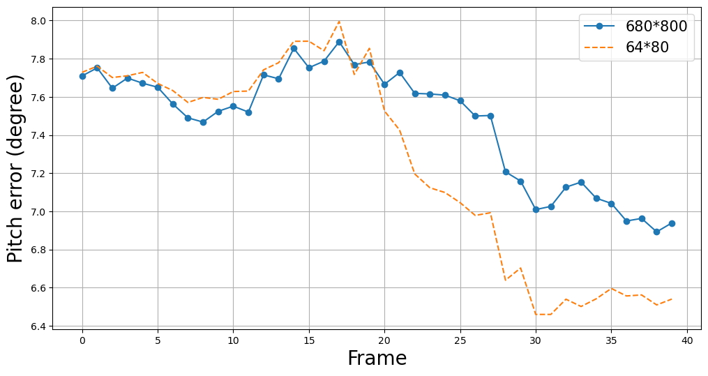
(a) SSIM

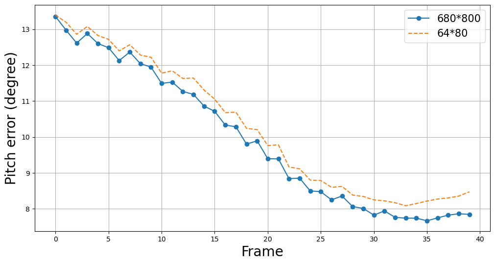
(b) CW-SSIM

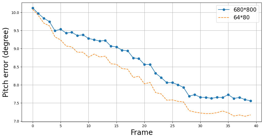
(c) LPIPS

Figure 13: (a) The comparison of average rotation error in the pitch of 20 trails at each frame when using SSIM in different resolutions. (b) The comparison of average rotation error in the pitch of 20 trails at each frame when using CW-SSIM in different resolutions. (c) The comparison of average rotation error in the pitch of 20 trails at each frame when using LPIPS in different resolutions.

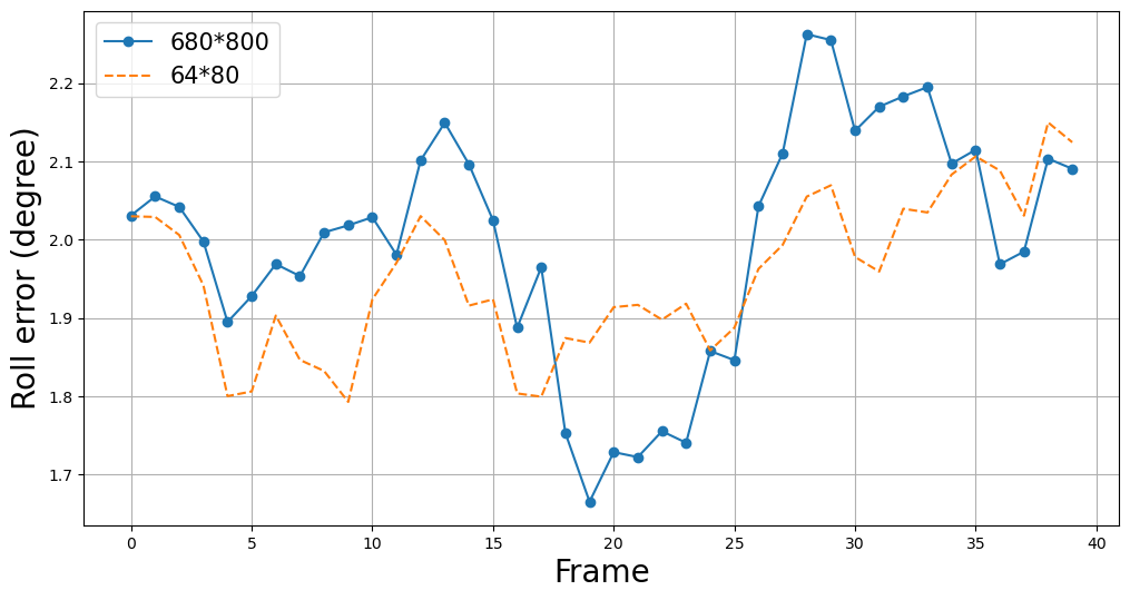
(a) SSIM

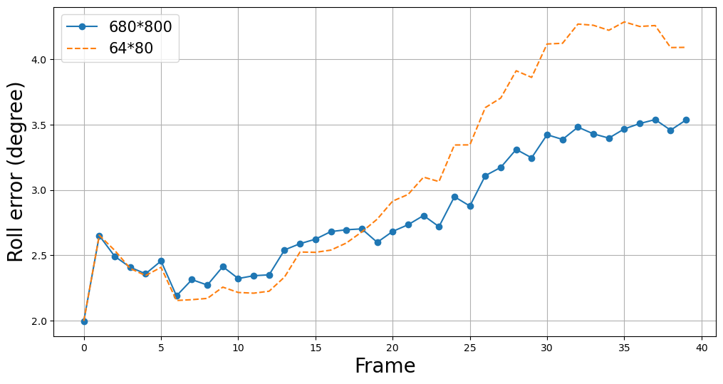
(b) CW-SSIM

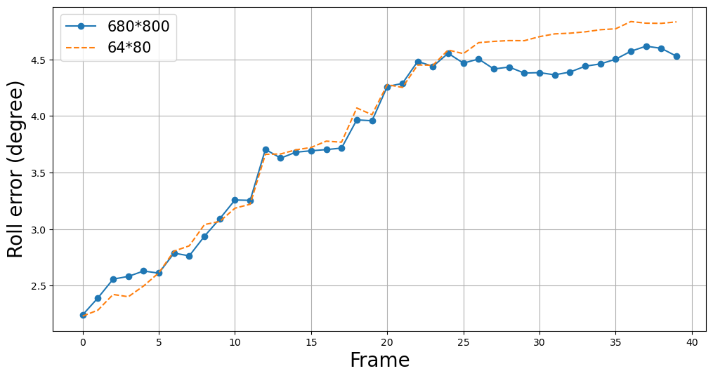
(c) LPIPS

Figure 14: (a) The comparison of average rotation error in the roll of 20 trails at each frame when using SSIM in different resolutions. (b) The comparison of average rotation error in the roll of 20 trails at each frame when using CW-SSIM in different resolutions. (c) The comparison of average rotation error in the roll of 20 trails at each frame when using LPIPS in different resolutions.

VI Conclusions and Future Study

We present NuRF, a nudged particle filter designed for robot visual localization in radiance fields. Our approach incorporates key insights, including visual place recognition for nudging and an adaptive scheme for both global localization and pose tracking. To evaluate the effectiveness of the NuRF framework, we perform real-world experiments and provide comparisons and ablated studies. These experiments serve to validate the effectiveness of NuRF in indoor environments.

We consider several promising directions that can be explored to advance NuRF. One potential direction is to investigate methods for determining the minimum number of anchors required to achieve satisfactory localization performance. Another promising direction is the integration of planning capabilities within the radiance fields, thus achieving full navigation with such implicit representations.

References

- [1] M. A. Fischler and R. C. Bolles, “Random sample consensus: a paradigm for model fitting with applications to image analysis and automated cartography,” Communications of the ACM, vol. 24, no. 6, pp. 381–395, 1981.
- [2] H. Yin, X. Xu, S. Lu, X. Chen, R. Xiong, S. Shen, C. Stachniss, and Y. Wang, “A survey on global lidar localization: Challenges, advances and open problems,” International Journal of Computer Vision, pp. 1–33, 2024.
- [3] S. Lowry, N. Sünderhauf, P. Newman, J. J. Leonard, D. Cox, P. Corke, and M. J. Milford, “Visual place recognition: A survey,” ieee transactions on robotics, vol. 32, no. 1, pp. 1–19, 2015.
- [4] S. Schubert, P. Neubert, S. Garg, M. Milford, and T. Fischer, “Visual place recognition: A tutorial,” IEEE Robotics & Automation Magazine, 2023.
- [5] J. Miao, K. Jiang, T. Wen, Y. Wang, P. Jia, B. Wijaya, X. Zhao, Q. Cheng, Z. Xiao, J. Huang et al., “A survey on monocular re-localization: From the perspective of scene map representation,” IEEE Transactions on Intelligent Vehicles, 2024.
- [6] F. Dellaert, D. Fox, W. Burgard, and S. Thrun, “Monte carlo localization for mobile robots,” in Proceedings 1999 IEEE international conference on robotics and automation (Cat. No. 99CH36288C), vol. 2. IEEE, 1999, pp. 1322–1328.
- [7] T. X. Lin, S. Coogan, D. A. Sofge, and F. Zhang, “A particle fusion approach for distributed filtering and smoothing,” Unmanned Systems, pp. 1–15, 2024.
- [8] Y. Xie, T. Takikawa, S. Saito, O. Litany, S. Yan, N. Khan, F. Tombari, J. Tompkin, V. Sitzmann, and S. Sridhar, “Neural fields in visual computing and beyond,” in Computer Graphics Forum, vol. 41, no. 2. Wiley Online Library, 2022, pp. 641–676.
- [9] D. Maggio, M. Abate, J. Shi, C. Mario, and L. Carlone, “Loc-nerf: Monte carlo localization using neural radiance fields,” in 2023 IEEE International Conference on Robotics and Automation (ICRA). IEEE, 2023, pp. 4018–4025.
- [10] B. Mildenhall, P. P. Srinivasan, M. Tancik, J. T. Barron, R. Ramamoorthi, and R. Ng, “Nerf: Representing scenes as neural radiance fields for view synthesis,” Communications of the ACM, vol. 65, no. 1, pp. 99–106, 2021.
- [11] G. Wang, L. Pan, S. Peng, S. Liu, C. Xu, Y. Miao, W. Zhan, M. Tomizuka, M. Pollefeys, and H. Wang, “Nerf in robotics: A survey,” arXiv preprint arXiv:2405.01333, 2024.
- [12] B. Kerbl, G. Kopanas, T. Leimkühler, and G. Drettakis, “3d gaussian splatting for real-time radiance field rendering,” ACM Transactions on Graphics, vol. 42, no. 4, pp. 1–14, 2023.
- [13] A. Hamdi, L. Melas-Kyriazi, G. Qian, J. Mai, R. Liu, C. Vondrick, B. Ghanem, and A. Vedaldi, “Ges: Generalized exponential splatting for efficient radiance field rendering,” arXiv preprint arXiv:2402.10128, 2024.
- [14] N. Keetha, J. Karhade, K. M. Jatavallabhula, G. Yang, S. Scherer, D. Ramanan, and J. Luiten, “Splatam: Splat, track & map 3d gaussians for dense rgb-d slam,” arXiv preprint arXiv:2312.02126, 2023.
- [15] P. Jiang, G. Pandey, and S. Saripalli, “3dgs-reloc: 3d gaussian splatting for map representation and visual relocalization,” arXiv preprint arXiv:2403.11367, 2024.
- [16] N. Keetha, A. Mishra, J. Karhade, K. M. Jatavallabhula, S. Scherer, M. Krishna, and S. Garg, “Anyloc: Towards universal visual place recognition,” IEEE Robotics and Automation Letters, vol. 9, no. 2, pp. 1286–1293, 2023.
- [17] P.-E. Sarlin, C. Cadena, R. Siegwart, and M. Dymczyk, “From coarse to fine: Robust hierarchical localization at large scale,” in Proceedings of the IEEE/CVF conference on computer vision and pattern recognition, 2019, pp. 12 716–12 725.
- [18] Ö. D. Akyildiz and J. Míguez, “Nudging the particle filter,” Statistics and Computing, vol. 30, pp. 305–330, 2020.
- [19] J. Nilsson and T. Akenine-Möller, “Understanding ssim,” arXiv preprint arXiv:2006.13846, 2020.
- [20] R. Zhang, P. Isola, A. A. Efros, E. Shechtman, and O. Wang, “The unreasonable effectiveness of deep features as a perceptual metric,” in Proceedings of the IEEE conference on computer vision and pattern recognition, 2018, pp. 586–595.
- [21] J.-Y. Zhu, P. Krähenbühl, E. Shechtman, and A. A. Efros, “Generative visual manipulation on the natural image manifold,” in Computer Vision – ECCV 2016, B. Leibe, J. Matas, N. Sebe, and M. Welling, Eds. Cham: Springer International Publishing, 2016, pp. 597–613.
- [22] M. Oquab, T. Darcet, T. Moutakanni, H. V. Vo, M. Szafraniec, V. Khalidov, P. Fernandez, D. Haziza, F. Massa, A. El-Nouby, R. Howes, P.-Y. Huang, H. Xu, V. Sharma, S.-W. Li, W. Galuba, M. Rabbat, M. Assran, N. Ballas, G. Synnaeve, I. Misra, H. Jegou, J. Mairal, P. Labatut, A. Joulin, and P. Bojanowski, “Dinov2: Learning robust visual features without supervision,” 2023.
- [23] Y. Gao, A. Rehman, and Z. Wang, “Cw-ssim based image classification,” in 2011 18th IEEE International Conference on Image Processing. IEEE, 2011, pp. 1249–1252.
- [24] Q. Tao, J. Wang, Z. Xu, T. X. Lin, Y. Yuan, and F. Zhang, “Swing-reducing flight control system for an underactuated indoor miniature autonomous blimp,” IEEE/ASME Transactions on Mechatronics, vol. 26, no. 4, pp. 1895–1904, 2021.