Error evaluation of partial scattering functions obtained from contrast variation small-angle neutron scattering

Abstract

Contrast variation small-angle neutron scattering (CV-SANS) is a powerful tool to evaluate the structure of multi-component systems by decomposing scattering intensities $I$ measured with different scattering contrasts into partial scattering functions $S$ of self- and cross-correlations between components. The measured $I$ contains a measurement error, $\Delta I$, and $\Delta I$ results in an uncertainty of partial scattering functions, $\Delta S$. However, the error propagation from $\Delta I$ to $\Delta S$ has not been quantitatively clarified. In this work, we have established deterministic and statistical approaches to determine $\Delta S$ from $\Delta I$. We have applied the two methods to experimental SANS data of polyrotaxane solutions with different contrasts, and have successfully estimated the errors of $S$. The quantitative error estimation of $S$ offers us a strategy to optimize the combination of scattering contrasts to minimize error propagation.

1 Introduction

Contrast variation small-angle neutron scattering (CV-SANS) has been utilized to study the nano-structure of multicomponent systems, such as organic/inorganic composite materials [NCgel, filled_rubber, CaCo3], self-assembled systems of amphipathic molecules [blockcopolymer, selfassemble], complexes of biomolecules  [protein, biological_membrane], and supramolecular systems [CVSANS_PR, model_PR]. For isotropic materials, 2-D SANS data is converted to 1-D scattering function $I(Q)$, where $Q$ is the magnitude of the scattering vector. In the case of $p$-components systems, the scattering function is a sum of partial scattering functions, $S_{ij}(Q)$ [CVSANS]:

$$I(Q)=\sum_{i=1}^{p}\rho_{i}^{2}S_{ii}(Q)+2\sum_{i<j}\rho_{i}\rho_{j}S_{ij}(Q)$$ (1)

where $\rho_{i}$ is the scattering length density of the $i$th component, $S_{ii}(Q)$ is a self-term corresponding to the structure of the $i$th component, and $S_{ij}(Q)$ is a cross-term originated from the correlation between the $i$th component and $j$th component. On the assumption of incompressibility, Eq. (1) can be reduced to the following equation [CVSANS]:

$$I(Q)=\sum_{i=1}^{p-1}(\rho_{i}-\rho_{p})^{2}S_{ii}(Q)+2\sum_{i<j}(\rho_{i}-\rho_{p})(\rho_{j}-\rho_{p})S_{ij}(Q).$$ (2)

For 3-components systems, in which two solutes ($i=1,2$) are dissolved in a solvent ($i=3$), the scattering function is given as below:

$$I(Q) =(\rho_{1}-\rho_{3})^{2}S_{11}(Q)+(\rho_{2}-\rho_{3})^{2}S_{22}(Q)+2(\rho_{1}-\rho_{3})(\rho_{2}-\rho_{3})S_{12}(Q)$$

$$=\Delta\rho_{1}^{2}S_{11}(Q)+\Delta\rho_{2}^{2}S_{22}(Q)+2\Delta\rho_{1}\Delta\rho_{2}S_{12}(Q)$$ (3)

Here, $\Delta\rho_{i}$ is the scattering length density difference between the $i$th solute and solvent. Based on Eq. (1), by measuring $I(Q)$’s of $N$ samples ($N\geq 3$) with different scattering contrasts ($\Delta\rho_{1}$ and $\Delta\rho_{2}$), it is possible to determine the three partial scattering functions, $S_{11}(Q)$, $S_{22}(Q)$, and $S_{12}(Q)$:

$$\begin{bmatrix}I_{1}\\ \vdots\\ I_{N}\end{bmatrix}=\begin{bmatrix}\Delta_{1}\rho_{1}^{2}&\Delta_{1}\rho_{2}^{2}&2\Delta_{1}\rho_{1}\Delta_{1}\rho_{2}\\ \vdots&\vdots&\vdots\\ \Delta_{N}\rho_{1}^{2}&\Delta_{N}\rho_{2}^{2}&2\Delta_{N}\rho_{1}\Delta_{N}\rho_{2}\end{bmatrix}\begin{bmatrix}S_{11}\\ S_{22}\\ S_{12}\end{bmatrix}$$ (4)

From the calculated partial scattering functions, we can analyze the structure of each solute and cross-correlation between the two solutes. Despite the usefulness of CV-SANS, its application has been limited due to the complexity and uncertainty of the calculation. The experimentally obtained $I(Q)$ has a statistical error $\Delta I$, and therefore we should consider how $\Delta I$ propagates to the error of $S(Q)$:

$$\begin{bmatrix}I_{1}+\Delta I_{1}\\ \vdots\\ I_{N}+\Delta I_{N}\end{bmatrix}=\begin{bmatrix}\Delta_{1}\rho_{1}^{2}&\Delta_{1}\rho_{2}^{2}&2\Delta_{1}\rho_{1}\Delta_{1}\rho_{2}\\ \vdots&\vdots&\vdots\\ \Delta_{N}\rho_{1}^{2}&\Delta_{N}\rho_{2}^{2}&2\Delta_{N}\rho_{1}\Delta_{N}\rho_{2}\end{bmatrix}\begin{bmatrix}S_{11}+\Delta S_{11}\\ S_{22}+\Delta S_{22}\\ S_{12}+\Delta S_{12}\end{bmatrix}$$ (5)

However, as far as we know, the relationship between $\Delta I$ and $\Delta S$ has not been clarified. The contribution of this study is an estimation of the transition from $\Delta I$ to $\Delta S$. To achieve this, we adopted two approaches: deterministic and statistical error estimations.

The objective of deterministic error estimation is to analytically estimate the upper bounds of $|\Delta S_{11}|$, $|\Delta S_{12}|$, and $|\Delta S_{22}|$ in Eq. (5). This essentially amounts to quantitatively clarifying the sensitivity of $S$ to the variations in $I$. It is essential to recognize this relationship, because it has a direct impact on the precision required for observing $I$. Theoretically, solving a least square problem is equivalent to multiplying its right-hand side vector by the Moore-Penrose inverse (e.g., [GV]), which is a kind of generalized inverse of its coefficient matrix. Therefore, the Moore-Penrose inverse plays a vital role in this analysis, enabling a detailed examination of the impact of each input variable. This sheds light on the complex pathways of error propagation within a system. Such an error estimation has already been done in the contexts of verified numerical computation (see [M], e.g.), and its effectiveness has been confirmed.

The objective of statistical error estimation is to establish the probabilistic description of $\Delta S$ from data under some statistical assumptions. Statisticians have long considered the problem of error estimation, such as interval estimation [intro_stat] and Bayesian statistics [bayesian_stat]. Recently, this field has been referred to as uncertainty quantification [uqtextbook] and has been widely studied. This study applies basic Bayesian inference with a noninformative prior distribution to estimate $\Delta S$. The estimation assumes that the error in $I$, namely $\Delta I$, follows a normal distribution. The framework is also used to examine the robustness of the estimation.

These approaches effectively capture the inherent uncertainties in the observational errors. The error bounds are accurately derived from the mathematical structure of Eq. (4), thereby offering significant insights into the reliability and precision of the computational results for the partial scattering functions. In this study, we applied our error estimation methods to the CV-SANS data of polyrotaxane solutions [CVSANS_PR]. Polyrotaxane is a topological supramolecular assembly, in which ring molecules are threaded onto a linear polymer chain. In our previous work, we performed contrast variation SANS measurements of polyrotaxane solutions to calculate their partial scattering functions. However, the errors of the obtained partial scattering functions were not fully evaluated. This study demonstrates the effectiveness of our method in quantifying uncertainties arising from the randomness of observational errors. In both error estimation approaches, the condition number of the coefficient matrix is a useful tool (see Sections 2.1 and 2.2 for detail).

2 Methods

2.1 Deterministic error estimation

Despite the usefulness of CV-SANS, its application has been limited due to the statistical error $\Delta I$ associated with the experimentally obtained $I(Q)$. It is not well-studied how $\Delta I$ propagates to the error of $S(Q)$. To address this issue, this subsection presents a theory that clarifies how $\Delta I$ propagates to the error of $S(Q)$, $\Delta S$, in a deterministic sense.

Define

$$I :=\begin{bmatrix}I_{1}\\ \vdots\\ I_{N}\end{bmatrix},\quad\Delta I:=\begin{bmatrix}\Delta I_{1}\\ \vdots\\ \Delta I_{N}\end{bmatrix},\quad A:=\begin{bmatrix}\Delta_{1}\rho_{1}^{2}&\Delta_{1}\rho_{2}^{2}&2\Delta_{1}\rho_{1}\Delta_{1}\rho_{2}\\ \vdots&\vdots&\vdots\\ \Delta_{N}\rho_{1}^{2}&\Delta_{N}\rho_{2}^{2}&2\Delta_{N}\rho_{1}\Delta_{N}\rho_{2}\end{bmatrix},$$ (6)

$$S :=\begin{bmatrix}S_{11}\\ S_{22}\\ S_{12}\end{bmatrix},\quad\Delta S:=\begin{bmatrix}\Delta S_{11}\\ \Delta S_{22}\\ \Delta S_{12}\end{bmatrix}.$$

Then, (5) can be written as

$$I+\Delta I=A(S+\Delta S).$$ (7)

It is obvious that $S$ and $\Delta S$ are 3-dimensional vectors, and $A$ is an $N\times 3$ matrix. Sections 2.1 and 2.2 generalize Eq. (5), and treat the case where $S$ and $\Delta S$ are $m$-dimensional vectors, and $A$ is a $N\times m$ matrix. To this end, we introduce notations used in Sections 2.1 and 2.2. For $v\in\mathbb{R}^{n}$, let $v_{i}$ for $i=1,\dots,n$ be the $i$-th component of $v$, and $\|v\|:=\sqrt{v_{1}^{2}+\cdots+v_{n}^{2}}$. For $v,w\in\mathbb{R}^{n}$, the inequality $v\leq w$ means that $v_{i}\leq w_{i}$ holds for all $i$. Let $\mathbb{R}^{n}_{\geq 0}:=\{v\in\mathbb{R}^{n}\ |\ v\geq 0\}$. For $B\in\mathbb{R}^{m\times n}$, let $b_{ij}$ and $\|B\|$ be the $(i,j)$ element and 2-norm (see [GV], e.g.) of $B$, respectively. Suppose $v\leq w$, and define

$$[v,w]:=\left(\begin{array}[]{c}[v_{1},w_{1}]\\ \vdots\\ {[}v_{n},w_{n}{]}\\ \end{array}\right),\quad|v|:=\left(\begin{array}[]{c}|v_{1}|\\ \vdots\\ |v_{n}|\end{array}\right),\quad|B|:=\left(\begin{array}[]{ccc}|b_{11}|&\cdots&|b_{1n}|\\ \vdots&\ddots&\vdots\\ |b_{n1}|&\cdots&|b_{nn}|\\ \end{array}\right).$$

Denote the Moore-Penrose inverse of $B$ by $B^{+}$. When $m\geq n$ and $B$ has full column rank in particular, we have $B^{+}=(B^{T}B)^{-1}B^{T}$, where $B^{T}$ denotes the transpose of $B$.

We present Theorem 1 for clarifying how $\Delta I$ propagates to $\Delta S$ in a deterministic sense. See Appendix A for its proof. Theorem 1 says that we can analytically estimate an upper bound on $|\Delta S|$.

Theorem 1.

Let $A\in\mathbb{R}^{N\times m}$, $I,\Delta I\in\mathbb{R}^{N}$, $\Delta J\in\mathbb{R}^{N}_{\geq 0}$, $S,\Delta S\in\mathbb{R}^{m}$, and $\Delta T:=|A^{+}|\Delta J$. Suppose that $N\geq m$, $AS=I$, $I+\Delta I=A(S+\Delta S)$, $|\Delta I|\leq\Delta J$, and $A$ has full column rank. It then follows that

$$|\Delta S|\leq\Delta T.$$ (8)

Remark 1.

In practice, we regard the standard deviation of the experimentally obtained $I(Q)$ as $\Delta J$

Define the condition number ${\rm cond}(A)$ by ${\rm cond}(A):=\|A\|\|A^{+}\|$. Let $\lambda_{\max}$ and $\lambda_{\min}$ be the largest and smallest singular values of $A$, respectively. We then have $\|A\|=\lambda_{\max}$, $\|A^{+}\|=1/\lambda_{\min}$, so that ${\rm cond}(A)=\lambda_{\max}/\lambda_{\min}$. It can be shown by using the singular value decomposition (e.g., [GV]) of $A^{+}$ that $\|A^{+}I\|\geq\|I\|/\lambda_{\max}$. These relations and $S=A^{+}I$ give

$$\frac{\|\Delta T\|}{\|S\|}=\frac{\||A^{+}|\Delta J\|}{\|A^{+}I\|}\leq\frac{\|A^{+}\|\|\Delta J\|}{\|I\|/\lambda_{\max}}=\frac{\lambda_{\max}\|\Delta J\|}{\lambda_{\min}\|I\|}=\frac{{\rm cond}(A)\|\Delta J\|}{\|I\|}$$

if $S\neq 0$ and $I\neq 0$. This inequality implies that $\|\Delta T\|/\|S\|$ is enlarged by ${\rm cond}(A)$.

2.2 Statistical error estimation

To statistically quantify the estimation errors $\Delta S_{ij}$, we rewrite (5) into the following statistical model:

$$I+\Delta I=AS,$$ (9)

where

$$I :=\begin{bmatrix}I_{1}\\ \vdots\\ I_{N}\end{bmatrix},\ \Delta I:=\begin{bmatrix}\Delta I_{1}\\ \vdots\\ \Delta I_{N}\end{bmatrix},\ A:=\begin{bmatrix}\Delta_{1}\rho_{1}^{2}&\Delta_{1}\rho_{2}^{2}&2\Delta_{1}\rho_{1}\Delta_{1}\rho_{2}\\ \vdots&\vdots&\vdots\\ \Delta_{N}\rho_{1}^{2}&\Delta_{N}\rho_{2}^{2}&2\Delta_{N}\rho_{1}\Delta_{N}\rho_{2}\end{bmatrix},\ S:=\begin{bmatrix}S_{11}\\ S_{22}\\ S_{12}\end{bmatrix}.$$

In this formulation, $S_{ij}$ includes $\Delta S_{ij}$ since the values we want to estimate are considered random variables with a prior distribution in the Bayesian framework. The following assumptions are made to build the statistical model.

• Each $\Delta I_{i}$ is a normal random variable with mean zero and standard deviation $\sigma_{i}$

• $\Delta I_{1},\ldots,\Delta I_{N}$ are probabilistically independent

• The prior distribution of $S$ is a multivariate normal distribution $\mathcal{N}(0,\alpha^{2}E)$, where $\alpha>0$ is a parameter and $E$ is an $N\times N$ identity matrix

From the first two assumptions, $\Delta I$ is a multivariate normal random variable with mean zero and covariance matrix $\Sigma$, where

$$\Sigma=\begin{bmatrix}\sigma_{1}^{2}&&\\ &\ddots&\\ &&\sigma_{N}^{2}\end{bmatrix}.$$

Then the posterior distribution of $S$ is $\mathcal{N}(\bar{S}_{\alpha},\bar{\Sigma}_{\alpha})$ from Bayes’ formula for multivariate normal distributions [Section 6.1 in [uqtextbook]], where $\bar{\Sigma}_{\alpha}=(\alpha^{-2}E+A^{T}\Sigma^{-1}A)^{-1}$ and $\bar{S}_{\alpha}=\bar{\Sigma}_{\alpha}A^{T}\Sigma^{-1}I$. The prior distribution represents the assumption on the scale of $S$, and we try to remove the effect of the assumption using noninformative prior by $\alpha\to+\infty$. As a result, the posterior distribution of $S$ is $\mathcal{N}(\bar{S},\bar{\Sigma})$, where

$$\bar{\Sigma}_{\alpha}\to\bar{\Sigma} =(A^{T}\Sigma^{-1}A)^{-1},$$ (10)

$$\bar{S}_{\alpha}\to\bar{S} =\bar{\Sigma}A^{T}\Sigma^{-1}I.$$

By setting

$$\bar{S}=\begin{bmatrix}\bar{S}_{11}\\ \bar{S}_{22}\\ \bar{S}_{12}\end{bmatrix},\text{ and }\bar{\Sigma}=\begin{bmatrix}\bar{\sigma}_{11,11}&\bar{\sigma}_{11,22}&\bar{\sigma}_{11,12}\\ \bar{\sigma}_{22,11}&\bar{\sigma}_{22,22}&\bar{\sigma}_{22,12}\\ \bar{\sigma}_{12,11}&\bar{\sigma}_{12,22}&\bar{\sigma}_{12,12}\end{bmatrix},$$ (11)

the result can be interpreted as follows:

• The posterior distribution of $S_{11}$ is a normal distribution with mean $\bar{S}_{11}$ and variance $\bar{\sigma}_{11,11}$. This means that $\bar{S}_{11}$ is the most likely value of $S_{11}$, but the uncertainty of the estimation is described by the normal distribution whose variance is $\bar{\sigma}_{11,11}$

• $S_{22}$ and $S_{12}$ can be also evaluated in the same way

• A non-diagonal element of $\bar{\Sigma}$ is the covariance of estimated values; that is, the estimated values are correlated

We remark that $\bar{S}$ differs from the solution of the standard least square problem, $A^{+}I$. In fact, $\bar{S}$ is the solution of the weighted least square problem: $\mathrm{argmin}_{S}\left\|\Sigma^{-1}(I-AS)\right\|$. This formula means that $\sigma_{j}$ quantifies the reliability of measurements, and squared errors are weighted by the reliability factors.

The following theorem is useful for estimating the error before an experiment since singular values can be calculated only from $A$. See Appendix A for its proof.

Theorem 2.

$\sqrt{|\text{an element of }\bar{\Sigma}|}\leq(1/\lambda_{\min})\max_{j}\Delta I_{j}$, where $\lambda_{\min}$ is the smallest singular value of the matrix $A$.

Because the diagonal elements of $\bar{\Sigma}$ are the standard deviations of $S_{11},S_{22}$, and $S_{12}$, we can say that the absolute error is roughly scaled by $1/\lambda_{\min}$. Because the observation $I$ is roughly equal to $A\bar{S}$, we can estimate the relation between $\|I\|$ and $\|\bar{S}\|$ as follows:

$$\|I\|\approx\|A\bar{S}\|\leq\|A\|\|\bar{S}\|=\lambda_{\max}\|\bar{S}\|,$$ (12)

where $\lambda_{\max}$ is the largest singular value of the matrix $A$. This means that $\|\bar{S}\|$ is approximately bounded by $\|I\|/\lambda_{\max}$ from below, and we can say that the relative error is roughly scaled by $\lambda_{\max}/\lambda_{\min}=\mathrm{cond}(A)$. This suggests that condition numbers are useful for estimating the relative errors from the viewpoint of Bayesian statistics.

Using the formulation, we can examine the robustness of the estimation. The assumptions on model (9) are not perfect, and real measurement has unknown error factors, such as the uncertainty of the scattering length density, deviation of the noise distribution from the normal distribution, and unknown bias of the measurement device. Of course, such errors are expected to be very small, but if these small errors significantly disturb the result, the estimated result will not be reliable.

One of the simplest ways to check the robustness of the result is to extend the error bars of the measurement virtually. Here, we consider what happened when $\sigma_{1},\ldots,\sigma_{N}$ are multiplied by $\mu>1$. In this case, $\Sigma$ is multiplied by $\mu^{2}$ in (10), and as a result $\bar{\Sigma}$ is multiplied by $\mu^{2}$ but $\bar{S}$ is not changed. Therefore, the standard deviations of the posterior distributions are multiplied by $\mu$, which means that the estimation’s uncertainty is enlarged by $\mu$.

2.3 SANS data of polyrotaxane solutions

The deterministic and statistical error estimation methods are applied to the CV-SANS data of polyrotaxane (PR) solutions  [CVSANS_PR]). For the CV-SANS measurements, we used PR consisting of polyethylene glycol (PEG) as a liner polymer chain and $\alpha$-cyclodextrins (CDs) as rings. According to Eq.(1), the measured scattering intensities $I(Q)^{\prime}s$ of the PR solutions are represented by three partial scatterings:

$$I(Q)=\Delta\rho_{\rm c}^{2}S_{\rm cc}(Q)+\Delta\rho_{p}^{2}S_{\rm pp}(Q)+2\Delta\rho_{\rm c}\Delta\rho_{\rm p}S_{\rm cp}(Q)$$ (13)

Here, $S_{\rm cc}(Q)$ is the self-term of CD, $S_{\rm pp}(Q)$ is the self-term of PEG, and $S_{\rm cp}(Q)$ is the cross-term of CD and PEG, as shown in Fig. 1. For the CV-SANS measurements, eight PR solutions with different scattering contrasts were used. The sample list is shown in Table 1. Two types of PR were synthesized: h-PR, composed of CD and hydrogenated PEG (h-PEG), and d-PR, composed of CD and deuterated PEG (d-PEG). The scattering-length densities $\rho$ of h-PEG, d-PEG, and CD were $0.65\times 10^{10}$, $7.1\times 10^{10}$, and $2.0\times 10^{10}$ cm^-2, respectively. h-PR and d-PR were dissolved in mixtures of dimethyl sulfoxide (DMSO) and deuterated DMSO. The volume fraction of PR in the solutions was 8%. The volume fractions of deuterated DMSO in the solvent, $\phi_{d}$ were 1.0, 0.95, 0.90, and 0.85, and the corresponding scattering-length densities of the solvents were $5.3\times 10^{10}$, $5.0\times 10^{10}$, $4.7\times 10^{10}$, and $4.5\times 10^{10}$ cm^-2, respectively. In Table 1, $\Delta\rho_{p}$ and $\Delta\rho_{c}$, corresponding to scattering contrasts of PEG and CD, are summarized.

The scattering intensities of the eight PR solutions were measured by SANS [CVSANS_PR]). SANS measurements of the PR solutions were performed at 298 K by using the SANS-U diffractometer of the Institute for Solid State Physics, The University of Tokyo, located at the JRR-3 research reactor of the Japan Atomic Energy Agency in Tokai, Japan. The incident beam wavelength was 7.0 Å, and the wavelength distribution was 10%. Sample-to-detector distances were 1 and 4 m, and the covered $Q$ range was $0.01\AA^{-1}<Q<0.3\AA^{-1}$. The scattered neutrons were collected with a two-dimensional detector and then the necessary corrections were made, such as air and cell scattering subtractions. After these corrections, the scattered intensity was normalized to the absolute intensity using a standard polyethylene film with known absolute scattering intensity. The two-dimensional intensity data were circularly averaged and the incoherent scattering was subtracted. The aravaged $I(Q)$’s of h-PR and d-PR solutions obtained by the SANS measurements are shown in Fig. 2. The error bars in Fig. 2 represent $\Delta I$ = $\pm\sigma$, in which $\sigma$ is the standard deviation of the circular averaged scattering intensity.

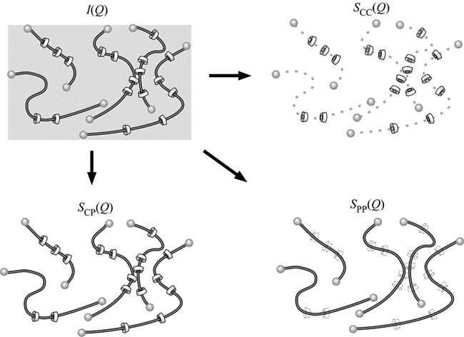
Figure 1: Schematic representations of polyrotaxane in solution showing the decomposition of scattering intensity $I(Q)$ into three partial scattering functions: self-term of PEG, $S_{\rm pp}(Q)$; self-term of CD, $S_{\rm cc}(Q)$; and a cross-term of PEG and CD, $S_{\rm cp}(Q)$.Reproduced from  [CVSANS_PR] with permission from American Chemical Society.

Table 1: Sample names, volume fractions of deuterated DMSO in the solvent, $\phi_{d}$, $\Delta\rho_{\rm c}$, and $\Delta\rho_{\rm p}$ of the PR solutions for the CV-SANS measurments.

Sample ID	PEG	$\phi_{d}$	$\Delta\rho_{\rm c}$ /$10^{10}$cm-2	$\Delta\rho_{\rm p}$ /$10^{10}$cm-2
h100	h-PEG	1.0	-3.3	-4.7
h095	h-PEG	0.95	-3.0	-4.4
h090	h-PEG	0.90	-2.7	-4.1
h085	h-PEG	0.85	-2.5	-3.9
d100	d-PEG	1.0	-3.3	1.8
d095	d-PEG	0.95	-3.0	2.1
d090	d-PEG	0.90	-2.7	2.4
d085	d-PEG	0.85	-2.5	2.6

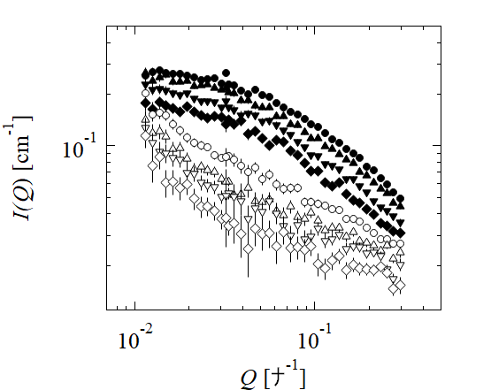
Figure 2: Scattering intensities of h-PR (solid symbols) and d-PR (open symbols) in mixtures of DMSO-d6 and DMSO. Circles ($\bullet$,$\circ$), upward triangles ($\blacktriangle$,$\vartriangle$), downward triangles ($\blacktriangledown$,$\triangledown$), and diamonds ($\blacklozenge$,$\lozenge$) correspond to $\phi_{\text{DMSO-d6}}=1.0$, $0.95$, $0.90$, and $0.85$, respectively, where $\phi_{\text{DMSO-d6}}$ is the volume fraction of DMSO-d6 in the solvent. The errors in $I(Q)$ are $\pm$ one standard deviations of the scattering intensities calculated during the circular averaging. Reproduced from  [CVSANS_PR] with permission from American Chemical Society.

3 Results

In this section, we report numerical results for the error estimations presented in Section 2. Specifically, Subsections 3.1 and 3.2 show the results for the estimations presented in Subsections 2.1 and 2.2, respectively.

This section considers the case when $S_{11}$, $S_{22}$, $S_{12}$, $\Delta_{i}\rho_{1}$, and $\Delta_{i}\rho_{2}$ for $i=1,\dots,N$ in Eq. (5) are $S_{\rm cc}$, $S_{\rm pp}$, $S_{\rm cp}$, $\Delta\rho_{\rm c}$, and $\Delta\rho_{\rm p}$, respectively, as defined in Subsection 2.3.

3.1 Results for the deterministic error estimation

For $c\in\mathbb{R}^{n}$ and $r\in\mathbb{R}^{n}_{\geq 0}$, define $\langle c,r\rangle:=[c-r,c+r]$. Let $I$, $\Delta I$, $A$, $S$, and $\Delta S$ be as in (6). We generated $I+\Delta I$ and $A$ based on the data in Subsection 2.3. As mentioned in Remark 1, we regarded the standard deviation of the experimentally obtained $I(Q)$ as $\Delta J$ in Theorem 1. Then, the interval $\langle I+\Delta I,\Delta J\rangle$ contains $I$ with the probability about 68.3% if $I$ follows a normal distribution. Because $\Delta T$ in Theorem 1 is the upper bound on $|\Delta S|$, the interval $\langle S+\Delta S,\Delta T\rangle$ contains $S$ a the probability equal to or larger than 68.3% in this case. If $I\in\langle I+\Delta I,\Delta J\rangle$ holds rigorously, then so does $S\in\langle S+\Delta S,\Delta T\rangle$.

Denote the upper bounds on $|\Delta S_{\rm cc}|$, $|\Delta S_{\rm pp}|$, and $|\Delta S_{\rm cp}|$ obtained based on Theorem 1 by $\Delta T_{\rm cc}$, $\Delta T_{\rm pp}$, and $\Delta T_{\rm cp}$, respectively. Fig. 3 displays numerically computed $S_{\rm cc}+\Delta S_{\rm cc}$, $S_{\rm pp}+\Delta S_{\rm pp}$, $S_{\rm cp}+\Delta S_{\rm cp}$, $\Delta T_{\rm cc}$, $\Delta T_{\rm pp}$, and $\Delta T_{\rm cp}$ for various $Q$. Fig. 4 reports $\Delta T_{\rm cc}/(S_{\rm cc}+\Delta S_{\rm cc})$, $\Delta T_{\rm pp}/(S_{\rm pp}+\Delta S_{\rm pp})$, and $\Delta T_{\rm cp}/(S_{\rm cp}+\Delta S_{\rm cp})$ for various $Q$.

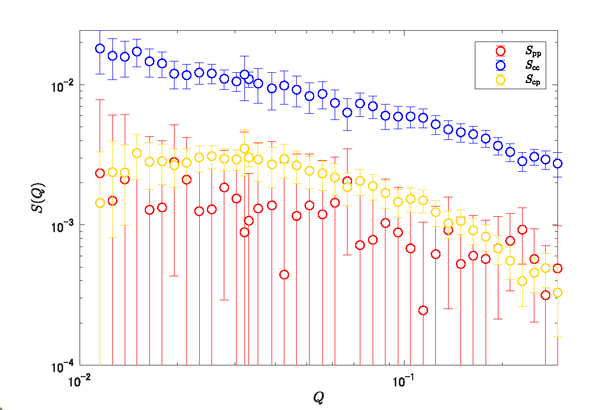
Figure 3: Numerically computed $S_{\rm cc}+\Delta S_{\rm cc}$, $S_{\rm pp}+\Delta S_{\rm pp}$, $S_{\rm cp}+\Delta S_{\rm cp}$, $\Delta T_{\rm cc}$, $\Delta T_{\rm pp}$, and $\Delta T_{\rm cp}$ for various $Q$. The circles stand for $S_{\rm cc}+\Delta S_{\rm cc}$, $S_{\rm pp}+\Delta S_{\rm pp}$, or $S_{\rm cp}+\Delta S_{\rm cp}$. The half lengths of the vertical line-segments denote $\Delta T_{\rm cc}$, $\Delta T_{\rm pp}$, or $\Delta T_{\rm cp}$.

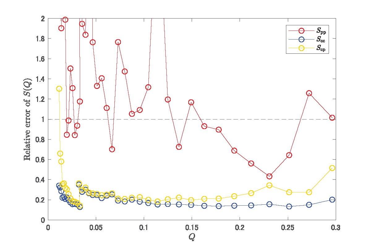
Figure 4: Numerically computed relative errors $\Delta T_{\rm cc}/(S_{\rm cc}+\Delta S_{\rm cc})$, $\Delta T_{\rm pp}/(S_{\rm pp}+\Delta S_{\rm pp})$, and $\Delta T_{\rm cp}/(S_{\rm cp}+\Delta S_{\rm cp})$ for various $Q$.

We see from Fig.s 3 and 4 that, for all $Q$, the error bound $\Delta T_{\rm pp}$ is much larger than $\Delta T_{\rm cc}$ and $\Delta T_{\rm cp}$. This result shows that $S_{\rm pp}+\Delta S_{\rm pp}$ is less reliable than $S_{\rm cc}+\Delta S_{\rm cc}$ and $S_{\rm cp}+\Delta S_{\rm cp}$. It can be observed that $\Delta T_{\rm cp}$ is large when $Q$ is the largest or smallest, whereas it is small in the other cases. The positive cross-term $S_{\rm cp}$ represents the topologically connection between CD and PEG  [CVSANS_PR, model_PR]. $S_{\rm cc}$ corresponding to the alignment of CDs on PEG can be described by a random copolymer model  [model_PR].

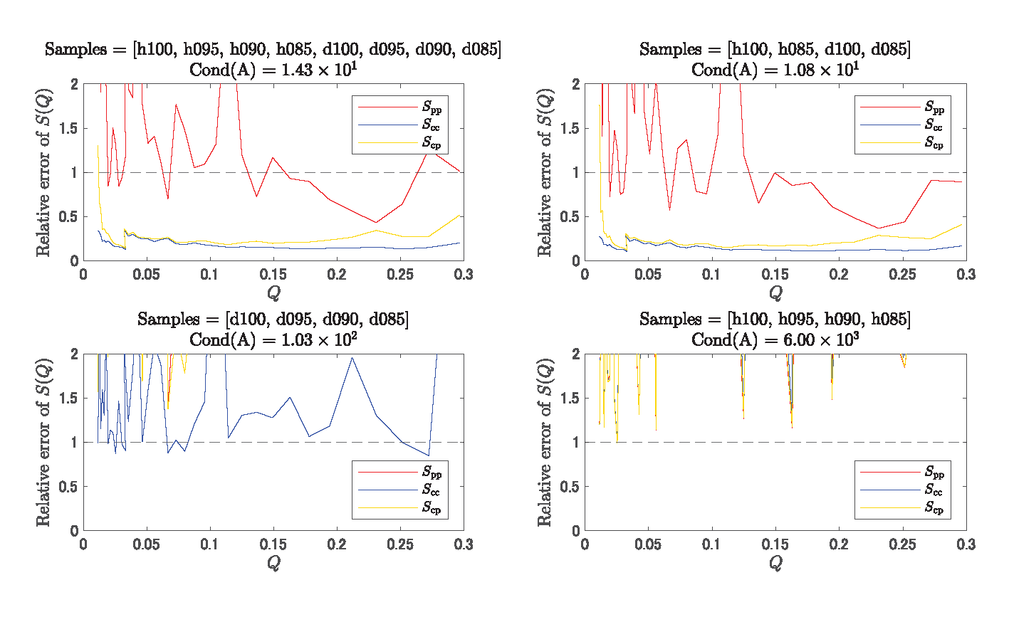
Figure 5: Comparison of relative errors in estimating $S_{\rm cc}$, $S_{\rm pp}$, and $S_{\rm cp}$ using different combinations of samples in Table 1.

The least-squares problem (4) consists of $N$ equations; however, to determine the three variables $S_{\rm cc}$, $S_{\rm pp}$, and $S_{\rm cp}$, selecting three or more of these equations is mathematically sufficient. However, using all available equations does not always yield the best error estimation. As previously mentioned, minimizing the condition number of $A$, as per Theorem 1, provides better deterministic error estimation.

Fig. 5 compares the errors of four different combinations of equations selected from the eight available. The vertical axis represents the relative error with respect to $S$. A relative error exceeding 1 implies that the error exceeds 100% of the true value, indicating that the results are unreliable unless the numbers are below this threshold.

The combination of samples h100, h085, d100, and d085 located at the top right, provided the best error estimation. This combination corresponds to selecting the two with the most distinct deuteration levels (i.e., contrast) from each PEG. Surprisingly, this resulted in smaller errors than capturing all samples located at the top left. However, it is important to note that statistical error estimation can yield more statistically significant confidence intervals with more equations, indicating that these results may not always align. See Subsection 3.2 and Fig. 8 for more details.

The bottom two combinations, which only altered the deuteration level of the solution using one type of PEG, resulted in relatively large condition numbers for $A$, and consequently, relative errors exceeding 1 for each S.

3.2 Results for statistical error estimation

We applied the method described in Section 2.2 to the SANS data by setting $I_{1},\ldots,I_{N}$ to the circular averaged scattering intensities and $\sigma_{1},\ldots,\sigma_{N}$ to the standard deviations of the circular averages. Fig. 6 shows the estimated partial scattering functions and estimated errors computed by (10). The error bars show $\bar{S}_{\rm cc}\pm\bar{\sigma}_{\rm cc},\ \bar{S}_{\rm pp}\pm\bar{\sigma}_{\rm pp}$ and $\bar{S}_{\rm cp}\pm\bar{\sigma}_{\rm cp}$, where $\bar{\sigma}_{\rm cc}=\sqrt{\bar{\sigma}_{\rm cc,\rm cc}}$, $\bar{\sigma}_{\rm pp}=\sqrt{\bar{\sigma}_{\rm pp,\rm pp}}$, and $\bar{\sigma}_{\rm cp}=\sqrt{\bar{\sigma}_{\rm cp,\rm cp}}$. Fig. 7 shows the relative estimated errors, that is, $\bar{\sigma}_{\rm cc}/\bar{S}_{\rm cc},\bar{\sigma}_{\rm pp}/\bar{S}_{\rm pp}$, and $\bar{\sigma}_{\rm cp}/\bar{S}_{\rm cp}$.

Using Bayesian inference, we can successfully evaluate the errors from the measurement data. From the result, we can say that the estimated $S_{\rm cc}$ and $S_{\rm cp}$ are relatively reliable, but $S_{\rm pp}$ is not completely reliable. The relative errors for $S_{\rm cc}$ are small for all $Q$, but the relative errors for $S_{\rm cp}$ are quite high for low-$Q$ and high-$Q$. For mid-$Q$, both $S_{\rm cc}$ and $S_{\rm cp}$ have small relative errors. We also say that the estimation of $S_{\rm cc}$ and $S_{\rm cp}$ for mid-$Q$ is quite robust using the robustness formula since the relative errors are less than 0.25 and a slight magnification of the errors (for example, $\times 1.2$) is not considered serious.

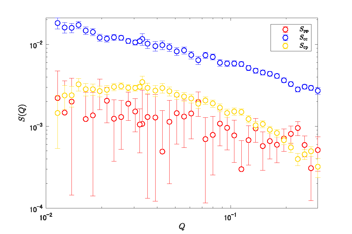
Figure 6: Estimated partial scattering functions and errors obtained through Bayesian inference. The error bars mean the standard deviations of the posterior distributions.

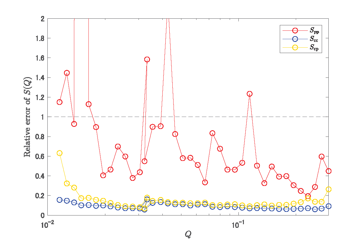
Figure 7: Relative estimated errors of the partial scattering functions obtained through Bayesian inference.

We apply the statistical method to the combinations of equations, as shown in Fig. 5. Fig. 8 displays the relative errors, which is consistent with the observations in Fig. 5. The combination of samples h100, h085, d100, and d085 (the top-right panel) exhibits relative error similar to those observed for all samples (the top-left panel). The finding suggests the utility of considering the condition number from the perspective of Bayesian inference. Indeed, the relative errors at the top right are slightly worse than at the top left, unlike in the deterministic case. This difference is likely due to the fact that, in statistical inference, both condition numbers and the amount of data influence the accuracy of the estimation.

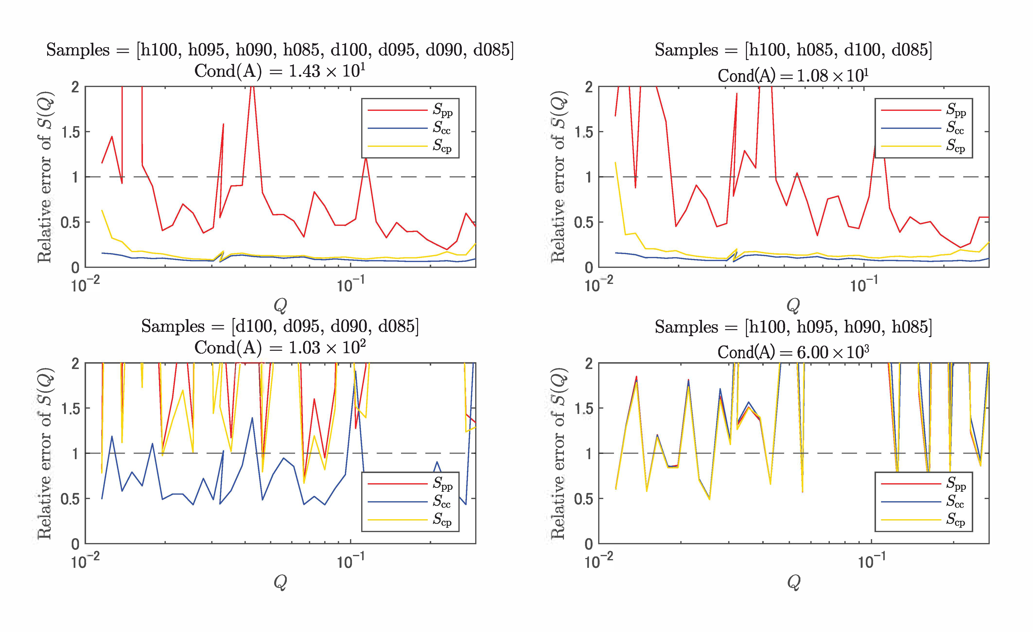
Figure 8: Comparison of relative errors by the Bayesian inference using different combinations of samples in Table 1.

4 Conclusion

In this study, we have established the deterministic and statistical error estimation methods for partial scattering functions obtained from scattering intensities of CV-SANS measurements. By applying these methods to CV-SANS data of polyrotaxane solutions, we successfully achieved theoretically grounded error estimations of their partial scattering functions. This approach is valuable for evaluating the reliability of partial scattering functions computed from CV-SANS data. Additionally, the error estimation can be used to optimize CV-SANS measurement conditions, such as scattering contrasts of samples and measurement times of the samples.

This study also highlighted the significance of the singular values of the matrix appearing on the right side of the problem (4) in predicting error bars of partial scattering functions. For both the deterministic and the statistical methods, the inverse of the minimum singular value, $1/\lambda_{\min}$, provides the scaling factor of absolute errors from CV-SANS measurements to the partial scattering functions, while the condition number, $\lambda_{\max}/\lambda_{\min}$, offers the scaling factor of relative errors. Because the singular values can be calculated only from scattering length densities $\rho_{i}$, the scaling factor can be estimated without CV-SANS measurements. Therefore, the singular values can aid in experimental design. For example, Figs. 5 and 8 demonstrate that only four CV-SANS experimental data provide almost the same error bars as all eight CV-SANS experimental data; this fact suggests the possibility of reducing experimental costs using condition numbers. A lower condition number indicates that a smaller $\Delta S$ is obtained for the same $\Delta I$, emphasizing the importance of exploring the choices of $\rho_{i}$ that minimizes this condition number. This exploration constitutes an intriguing aspect for future work.

5 Acknowledgments

This work is supported by the financial support of the JST FOREST Program (grant number JPMJFR2120). The SANS experiment was carried out by the JRR-3 general user program managed by the Institute for Solid State Physics, The University of Tokyo (Proposal No. 7607).

Appendix A Proof of Theorems

Proof of Theorem 1.

The assumptions $AS=I$ and $I+\Delta I=A(S+\Delta S)$ imply $A\Delta S=\Delta I$. Since $A$ has full column rank, we have $\Delta S=A^{+}\Delta I$, so $|\Delta I|\leq\Delta J$ yields

$$|\Delta S|=|A^{+}\Delta I|\leq|A^{+}||\Delta I|\leq\Delta T.$$

∎

Proof of Theorem 2.

Since $|\text{an element of }\bar{\Sigma}|\leq\|\bar{\Sigma}\|$, we will estimate the upper bound of $\|\bar{\Sigma}\|$. By using the minimal singular value, we have the following relation:

$$\|\bar{\Sigma}\|=\|{(A^{T}\Sigma^{-1}A)}^{-1}\|={(\text{minimal singular value of }A^{T}\Sigma^{-1}A)}^{-1}.$$

Since $A^{T}\Sigma^{-1}A$ is symmetric, the minimum singular value can be estimated as follows:

$$\text{minimum singular value of }A^{T}\Sigma^{-1}A =\min_{\|u\|=1}u^{T}A^{T}{(\sqrt{\Sigma})}^{-2}Au$$

$$=\min_{\|u\|=1}\|{(\sqrt{\Sigma})}^{-1}Au\|^{2}$$

$$\geq\min_{\|u\|=1}[(\min_{i}\sigma_{i}^{-2})\|Au\|^{2}]$$

$$\geq(\min_{i}\sigma_{i}^{-2})\lambda_{\min}^{2},$$

where

$$\sqrt{\Sigma}=\begin{bmatrix}\sigma_{1}&&\\ &\ddots&\\ &&\sigma_{N}\end{bmatrix}.$$

The above inequality provides the desired inequality.

∎

References

- [1] \harvarditemDekking2005intro_stat Dekking, F. \harvardyearleft2005\harvardyearright. A Modern Introduction to Probability and Statistics: Understanding Why and How. Springer Texts in Statistics. Springer.
- [2] \harvarditemEndo2006CVSANS Endo, H. \harvardyearleft2006\harvardyearright. Physica B, \volbf385, 682–684.
- [3] \harvarditem[Endo et al.]Endo, Mayumi, Osaka, Ito \harvardand Shibayama2011model_PR Endo, H., Mayumi, K., Osaka, N., Ito, K. \harvardand Shibayama, M. \harvardyearleft2011\harvardyearright. Polym. J. \volbf43, 155–163.
- [4] \harvarditem[Endo et al.]Endo, Miyazaki, Haraguchi \harvardand Shibayama2008NCgel Endo, H., Miyazaki, S., Haraguchi, K. \harvardand Shibayama, M. \harvardyearleft2008\harvardyearright. Macromolecules, \volbf41, 5406–5411.
- [5] \harvarditem[Endo et al.]Endo, Schwahn \harvardand Cölfen2004CaCo3 Endo, H., Schwahn, D. \harvardand Cölfen, H. \harvardyearleft2004\harvardyearright. J. Chem. Phys. \volbf120, 9410–9423.
- [6] \harvarditem[Fanova et al.]Fanova, Sotiropoulos, Radulescu \harvardand Papagiannopoulos2024selfassemble Fanova, A., Sotiropoulos, K., Radulescu, A. \harvardand Papagiannopoulos, A. \harvardyearleft2024\harvardyearright. Polymers, \volbf16, 490.
- [7] \harvarditemGolub \harvardand Van Loan2013GV Golub, G. \harvardand Van Loan, C. \harvardyearleft2013\harvardyearright. Matrix Computations. Baltimore and London: The Johns Hopkins University Press, 4th ed.
- [8] \harvarditemHoff2009bayesian_stat Hoff, P. D. \harvardyearleft2009\harvardyearright. A First Course in Bayesian Statistical Methods. Springer Publishing Company, Incorporated, 1st ed.
- [9] \harvarditem[Jeffries et al.]Jeffries, Graewert, Blanchet, Langley, Whitten \harvardand Svergun2016protein Jeffries, C. M., Graewert, M. A., Blanchet, C. E., Langley, D. B., Whitten, A. E. \harvardand Svergun, D. I. \harvardyearleft2016\harvardyearright. Nature Prot. \volbf11, 2122–2153.
- [10] \harvarditem[Mayumi et al.]Mayumi, Osaka, Endo, Yokoyama, H., Shibayama \harvardand Ito2008CVSANS_PR Mayumi, K., Osaka, N., Endo, H., Yokoyama, H., Sakai, Y., Shibayama, M. \harvardand Ito, K. \harvardyearleft2008\harvardyearright. Macromolecules, \volbf41, 6480–6485.
- [11] \harvarditemMiyajima2014M Miyajima, S. \harvardyearleft2014\harvardyearright. Linear Algebra Appl. \volbf444, 28–41.
- [12] \harvarditem[Nickels et al.]Nickels, Chatterjee, Stanley, Qian, Cheng, Myles, Standaert, Elkins \harvardand Katsaras2017biological_membrane Nickels, J. D., Chatterjee, S., Stanley, C. B., Qian, S., Cheng, X., Myles, D. A., Standaert, R. F., Elkins, J. G. \harvardand Katsaras, J. \harvardyearleft2017\harvardyearright. PLoS Biol. \volbf15, e2002214.
- [13] \harvarditem[Richter et al.]Richter, Schneiders, Monkenbusch, Willner, Fetters, Huang, Lin, Mortensen \harvardand Farago1997blockcopolymer Richter, D., Schneiders, D., Monkenbusch, M., Willner, L., Fetters, L. J., Huang, J. S., Lin, M., Mortensen, K. \harvardand Farago, B. \harvardyearleft1997\harvardyearright. Macromolecules, \volbf120, 1053–1068.
- [14] \harvarditemSullivan2015uqtextbook Sullivan, T. J. \harvardyearleft2015\harvardyearright. Introduction to uncertainty quantification.
- [15] \harvarditem[Takenaka et al.]Takenaka, Nishitsuji, Amino, Ishikawa, Yamagchi \harvardand Koizumi2009filled_rubber Takenaka, M., Nishitsuji, S., Amino, N., Ishikawa, Y., Yamagchi, D. \harvardand Koizumi, S. \harvardyearleft2009\harvardyearright. Macromolecules, \volbf42, 308–311.
- [16]