Optimized reinitialization based level-set method within industrial context

Abstract

This paper presents a solver using the Level-Set method (Sussman et al. [1994]) for incompressible two phase flows with surface tension. A one fluid approach is adopted where both phases share the same velocity and pressure field. The Level Set method has been coupled with the Ghost Fluid Method (Fedkiw et al. [1999]). An efficient and pragmatic solution is proposed to avoid interface displacement during the reinitialization of the level-Set fields. A solver called LSFoam has been implemented in the OpenFOAM (Weller et al. [1998]) framework with consistent Rhie & Chow interpolation Cubero and Fueyo [2007]. This solver has been tested on several test cases covering different scales and flow configurations: rising bubble test case, Hysing et al. [2007], Rayleigh-Taylor instability simulations Puckett et al. [1997], Ogee spillway flow Erpicum et al. [2018], 3D dambreak simulation with a square cylinder obstacle Gomez-Gesteira [2013] and KVLCC2 steady resistance calculations Larsson et al. [2014]. Overall results are in excellent agreement with reference data and the present approach is very promising for moderate free surface deformations.

Keywords Level Set  $\cdot$ Free surface flow  $\cdot$ Ghost Fluid Method  $\cdot$ OpenFOAM

1 Introduction

When simulating free surface flows in an engineering framework, the Volume-of-Fluid method (VoF, Hirt and Nichols [1981]) is very popular due to its natural ability to preserve mass. Two families can be distinguished among the VoF methods : algebraic-like approaches (Boris and Book [1997], Muzaferija [1998]) and geometric approaches (DeBar [1974], Roenby et al. [2016]). One of the main drawbacks of VoF methods for small scale flows is the difficulty to compute interface curvatures due to the sharpness of the volume fraction field. The Level Set (LS, Sussman et al. [1994]) method is another way to capture the interface between two phases. The method is based on the function $\phi$, being the signed distance to the interface. Unlike the VoF method, the assessment of the interface curvature is more reliable due to the smooth nature of the function $\phi$. Moreover, with the LS approach, the distance to the interface is readily accessible, making it an approach of choice for the Ghost Fluid Method (GFM), Fedkiw et al. [1999]. To capture the interface motions, the LS function is advected in a velocity field. As soon as the tangential component of the normal velocity gradient is non zero, such a procedure will break the distance property of the Level Set function ($\left|\boldsymbol{\nabla}\phi\right|\neq 1$). This behavior will generate unacceptable mass variations. Hence, a reinitialization procedure, Sussman et al. [1994], is often used for recovering the signed distance property of the LS function. To limit mass variations, researchers traditionally use a combination of 5th order WENO spatial schemes Liu et al. [1994], and Runge Kutta (RK2 or RK3) temporal scheme for the resolution of both transport and reinitialization equations (Huang et al. [2007], Lalanne et al. [2015]). Even with this numerical treatment there is still no guarantee that mass will be conserved, Gu et al. [2018]. Moreover, even if WENO schemes have been promisingly used for unstructured grids (Martin and Shevchuk [2018], Gärtner et al. [2020]) they remain complex to use for industrial applications. Indeed, WENO schemes require low Courant numbers ($<1/3$ in 3D, Titarev and Toro [2004]) which can be very restricting to decrease the calculation time when only the steady state regime is of interest (typically for ship resistance assessment). The sub-cell fix method, Hartmann et al. [2010], Russo and Smereka [2000], has been developed to limit interface displacements during the reinitilization, but its application is limited to Cartesian grids. Moreover, Sun et al. [2010] have shown that the zero Level-Set can be disturbed even with the sub-cell fix method. Applications of the original approach of Sussman et al. [1994] for 3D industrial situations remain limited : Khosronejad et al. [2019], Park et al. [2005], Huang et al. [2007] and restricted to structured grids. Hence, the approach efficiency, accuracy, robustness and range of applications for such situations remain unclear. Hence, using the available literature, this work aims at building an efficient Level-Set/GFM solver for arbitrary polyhedral cells, with enhancements of the Level-Set method, and that preserves the original simplicity of the approach of Sussman et al. [1994]. The solver, deployed within 2nd order finite volume OpenFOAM framework Weller et al. [1998] and referred as LSFoam, is tested for various flow configurations :

• Rising bubble (Hysing et al. [2007]),

• Rayleigh-Taylor instability simulations (Puckett et al. [1997]),

• Ogee spillway flow (Erpicum et al. [2018]),

• 3D dambreak simulation (Gomez-Gesteira [2013]),

• KVLCC2 steady resistance calculations (Larsson et al. [2014])

2 Mathematical and numerical procedure

2.1 The Level-Set equation

The computational domain is divided into two pieces $\varOmega^{+}$ and $\varOmega^{-}$ separated by the interface $\Gamma$. Where $\varOmega^{+}$ and $\varOmega^{-}$ represent respectively the domain of heavy and light phases. For a given point $\boldsymbol{x}$, the Level-Set function $\phi(x)$ is defined by the shortest distance $d$ to the interface. It is signed depending on the point domains (1), so that both numerical transport and stability near the interface are improved by avoiding $\boldsymbol{\nabla}\phi$ discontinuities.

$$\phi(\boldsymbol{x})=\begin{cases}0&\boldsymbol{x}\in\Gamma\\ d(\boldsymbol{x})&\boldsymbol{x}\in\varOmega^{+}\\ -d(\boldsymbol{x})&\boldsymbol{x}\in\varOmega^{-}\end{cases}$$ (1)

A consequence of this definition is that $\forall x,\left|\boldsymbol{\nabla}\phi\right|=1$.

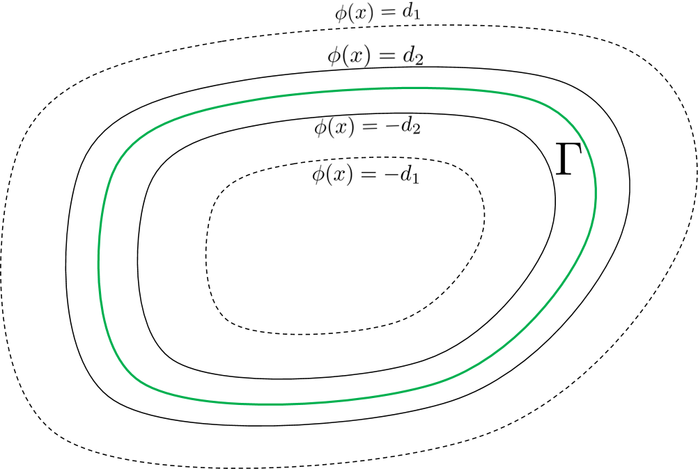
Figure 1: Illustration of the definition of the Level Set function. Each iso-contour $\left\{\boldsymbol{x}\mid\phi(\boldsymbol{x})=d\right\}$ define all the points $\boldsymbol{x}$ at a distance $d$ from the interface $\Gamma$.

Interface normal $\boldsymbol{n}$ and curvature $\kappa$ can be computed as follow:

$$\boldsymbol{n}=\frac{\boldsymbol{\nabla}\phi}{\left|\boldsymbol{\nabla}\phi\right|}$$ (2)

$$\kappa=\boldsymbol{\nabla}\cdot\boldsymbol{n}$$ (3)

The Level-Set function $\phi$ is advected in a flow field $\boldsymbol{u}$ (assumed incompressible) using a transport equation:

$$\frac{\partial\phi}{\partial t}+\boldsymbol{\nabla}\cdot(\boldsymbol{u}\phi)=0$$ (4)

The resolution of the transport equation is done with a sub-cycling strategy, Leroyer et al. [2011]. The time step is subdivided into $N$ sub-cycles enhancing mass conservation. However, the transport of the Level-Set function will breach the distance property and is likely to cause mass variations. To limit such consequences, a reinitialization procedure is adopted by solving the following (eikonal) equation (Sussman et al. [1994]):

$$\frac{\partial\phi}{\partial\tau}=S\left(\phi_{0}\right)\left(1-\left|\boldsymbol{\nabla}\phi\right|\right)$$ (5)

Where $S$ is the sign function, $\phi_{0}$ the initial value of the level set function and $\tau$ has the dimension of a length. The function $S$ is smoothed to improve the numerical resolution in the vicinity of the interface using the following expression Osher and Fedkiw [2003]:

$$S\left(\phi_{0}\right)=\frac{\phi_{0}}{\sqrt{\phi_{0}^{2}+\left|\boldsymbol{\nabla}\phi_{0}\right|\epsilon^{2}}}$$ (6)

The term $\left|\boldsymbol{\nabla}\phi_{0}\right|$ helps the reinitialization process when the initial field $\phi_{0}$ is away from the current level set field. $\epsilon$ can be a constant chosen as 2 or 3 times a user defined reference cell size. However, this can be prejudicial with non-uniform grids. To solve this issue, $\epsilon(x)$ becomes a variable computed on the domain for each cell $C(x)$ :

$$\epsilon(\boldsymbol{x})=kl_{e}$$ (7)

with k a user defined constant (usually $k=2$) and $l_{e}(x)$ the length of the edge so that :

$$\boldsymbol{l_{e}}\cdot\boldsymbol{n}=max(\boldsymbol{l_{e_{i}}}\cdot\boldsymbol{n}),\>\forall e_{i}\in C(x)$$

Kim and Park [2021] used an Euler explicit resolution of equation 5 based on the code of Yamamoto et al. [2017]. However, the explicit method has a limited range of applicability, especially for unstructured grids. Instead, Sussman et al. [1998] defined:

$$\boldsymbol{w}=S\left(\phi_{0}\right)\boldsymbol{n}$$ (8)

which leads to the following form of the reinitialization equation:

$$\frac{\partial\phi}{\partial\tau}+\boldsymbol{\nabla}\cdot(\boldsymbol{w}\phi)-\phi\boldsymbol{\nabla}\cdot\boldsymbol{w}=S\left(\phi_{0}\right)$$ (9)

Equation 9 is more suitable for implicit finite volume discretization Vukcevic and Jasak [2014], easing the use of unstructured meshes and improving the numerical stability. In this study, the reinitialization equation 9 is implicitly solved with the first order Euler scheme. The convective term $\boldsymbol{\nabla}\cdot(\boldsymbol{w}\phi)$ is discretized using 2nd order TVD MUSCL scheme, van Leer [1979]. The third term of equation 9 is treated implicitly. Authors generally use meshes with uniform cell size and define $\tau=0.5\Delta z$ where $\Delta z$ is the grid size. Nevertheless, for unstructured, highly distorted or non uniform meshes, used in industrial situations, this is not optimal as the cell size is likely to range from small near the walls to large in the far field region. We define the reinitialization Courant number $\gamma$ has:

$$\gamma(\boldsymbol{x})=\frac{\underset{f}{\sum}||\boldsymbol{w}_{f}||\tau}{V\left(\boldsymbol{x}\right)}$$ (10)

Where $V\left(\boldsymbol{x}\right)$ is the volume cell size and $\underset{f}{\sum}$ the face average operator. In practice, the magnitude of $\boldsymbol{w}$ is not always equal to 1, especially before reinitialization when $\phi$ can be far from the signed distance function or due to numerical errors. In this study, equation 9 is solved with a local time stepping approach (LTS) where the spatial time step $\tau$ is manipulated locally based on a given maximal reinitialization Courant number $\gamma_{max}$:

$$\frac{1.0}{\tau\left(\boldsymbol{x}\right)}=max\left(\frac{1.0}{\Delta z\left(\boldsymbol{x}\right)},\frac{\underset{f}{\sum}||\boldsymbol{w}_{f}||}{\gamma_{max}V\left(\boldsymbol{x}\right)}\right)$$ (11)

The above procedure allows to maximize the spatial time step for each cell based on $\gamma_{max}$ value. The spatial time step is limited by the local cell size $\Delta z\left(\boldsymbol{x}\right)$. In practice, interface displacements can occur during the reinitialization procedure leading to mass variations. If the reinitialization frequency and/or the iteration number are too important, strong interface displacements will occur. Traditionally, authors solve the eikonal equation for a given reinitialization frequency and for a number of iterations Henri [2021], Johansson [2011]. Hence, having to determine the optimal iteration number and frequency is the major drawback of this method. Moreover, these parameters are strongly case-dependent, and this is limiting its use for a wide range of complex situations.

To tackle all this, a simple and pragmatic solution that avoids any interface displacements during the resolution of the eikonal equation is proposed. The set of cells (called anchoring cells) crossing the zero Level-Set contour are detected. The corresponding Level-Set values are stored before the reinitialization procedure. Then, after each iteration of the eikonal equation resolution (reinitialization procedure), the anchoring cell Level-Set values are restored so that the zero Level-Set contour remains undisturbed during the reinitialization. This set of cells is constructed by grouping all the cells sharing the faces satisfying the criterion $\phi_{O}\phi_{N}<0$ ( equation 27). This method is then consistent with the GFM, that uses the same criterion to identify interface faces. The present approach is illustrated in 2 where the anchoring cells are colored in red. Level set contours are also plotted after reinitialization.

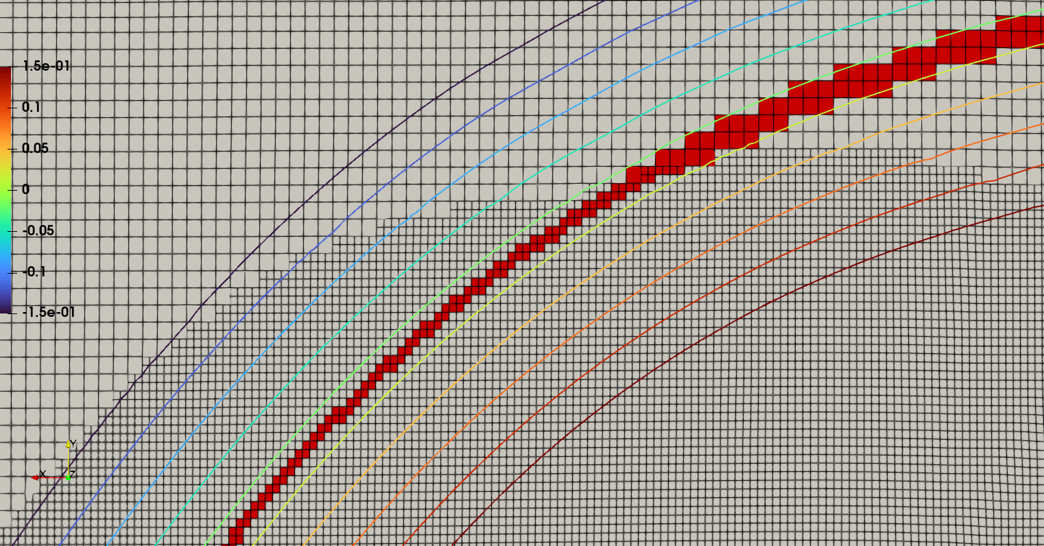
Figure 2: Illustration of the anchoring cells (coloured in red) used during the reinitialization procedure - level set contours are also plotted after reinitialization.

The Level-Set function is used to compute the phase fraction with a hyperbolic filtering function. The volume fraction $\alpha$ is calculated using the standard hyperbolic filtering function :

$$\alpha=\frac{1}{2}\left(tanh\left(\frac{\pi\phi}{\epsilon(\boldsymbol{x})}\right)+1\right)$$ (12)

The phase fraction $\alpha$ is then used to calculate the mixture viscosity $\mu$ as:

$$\mu=\alpha\mu^{+}+\left(1-\alpha\right)\mu^{-}$$ (13)

$$\begin{cases}\rho=\rho^{+}&if\;\phi>0\\ \rho=\rho^{-}&if\;\phi<0\end{cases}$$ (14)

Where $\mu^{+}$and $\mu^{-}$ are the dynamic viscosity of heavy and light phases and $\rho^{+}$ and $\rho^{-}$ their density.

2.2 Consistent pressure-velocity coupling

The momentum equation in each phase is given as follows, Trujillo [2021]:

$$\frac{\partial\boldsymbol{u}}{\partial t}+\boldsymbol{\nabla}\cdot(\boldsymbol{u}\cdot\boldsymbol{u})=\frac{1}{\rho}\left(-\boldsymbol{\nabla}p+\rho\boldsymbol{g}+\boldsymbol{\nabla^{2}}(\mu_{eff}\boldsymbol{u})+\boldsymbol{\nabla}\cdot\left[\mu_{eff}(\nabla\textbf{U})^{T}-\mu_{eff}\frac{2}{3}\mathrm{tr}(\nabla\textbf{U})^{T}\right]+\sigma\kappa\boldsymbol{n}\delta_{\Gamma}\right)$$ (15)

Where $\sigma$ is the surface tension coefficient, $\boldsymbol{n}$ the interface normal (equation 2), $\delta_{\Gamma}$ a surface Dirac function that equals one at the interface and zero otherwise and $\mu_{eff}$ the effective viscosity. In equation 15, the pressure is replaced by its decomposition into dynamic (or piezometric) $p_{d}$ and hydrostatic parts :

$$p=p_{d}+\rho\boldsymbol{g}\cdot\boldsymbol{x}$$ (16)

$$\boldsymbol{\nabla}p=\boldsymbol{\nabla}p_{d}+\boldsymbol{\nabla}\rho\boldsymbol{g}\cdot\boldsymbol{x}+\rho\boldsymbol{g}$$ (17)

The reason for using $p_{d}$ is to avoid any sudden changes of the pressure field at the boundaries for hydrostatic problems, Rusche [2002]. Then, assuming a piece-wise density field, the momentum balance takes the following form in each phase domain $\varOmega^{+}$ and $\varOmega^{-}$ :

$$\frac{\partial\boldsymbol{u}}{\partial t}+\boldsymbol{\nabla}\cdot(\boldsymbol{u}\cdot\boldsymbol{u})=\frac{1}{\rho}\left(\boldsymbol{\nabla}p_{d}+\boldsymbol{\nabla^{2}}(\mu_{eff}\boldsymbol{u})+\boldsymbol{\nabla}\cdot\left[\mu_{eff}(\nabla\textbf{U})^{T}-\mu_{eff}\frac{2}{3}\mathrm{tr}(\nabla\textbf{U})^{T}\right]\right),\;in\;\varOmega^{+}\;or\;\varOmega^{-}\;$$ (18)

Having a continuous velocity and dynamic viscosity fields, equation 18 is completed by the following set of jump conditions at the interface $\Gamma$:

$$\left[\frac{\boldsymbol{\nabla}p_{d}}{\rho}\right]_{\Gamma}=0$$ (19)

$$\left[p_{d}\right]_{\Gamma}=\sigma\kappa+\left[\rho\right]_{\Gamma}\boldsymbol{g}\cdot\boldsymbol{x}_{\Gamma}=\mathcal{H}$$ (20)

Where $\boldsymbol{x}_{\Gamma}$ is the interface coordinate vector. The bracket notation $\left[.\right]_{\Gamma}$ indicates a jump value between both sides of the interface. The momentum equation 18 is discretized without the pressure gradient term. The remaining terms are treated implicitly excepting $\frac{1}{\rho}\boldsymbol{\nabla}\cdot\left[\mu_{eff}(\nabla\textbf{U})^{T}-\mu_{eff}\frac{2}{3}\mathrm{tr}(\nabla\textbf{U})^{T}\right]$. The semi-discretized momentum equation takes the following form:

$$a_{p}\boldsymbol{u}_{p}=-\frac{\boldsymbol{\nabla}p_{d}}{\rho}-\underset{f}{\sum}a_{N}\boldsymbol{u}_{N}+\boldsymbol{s}(\boldsymbol{u})=-\frac{\boldsymbol{\nabla}p_{d}}{\rho}+\boldsymbol{H}(\boldsymbol{u}_{p})$$ (21)

The coefficient $a_{p}$ and $a_{N}$ are respectively the diagonal and off-diagonal terms of the discretized momentum equations. Explicit contributions are grouped in $\boldsymbol{H}(\boldsymbol{u})$. The summation stands for all the faces shared by the owner cell P and its neighboring cells N. To avoid checkerboard oscillations on collocated grids, the so-called Rhie and Chow [1983] interpolation is used to obtain the face velocity by mimicking Equation 21. In order to avoid relaxation factor and time step dependencies, the interpolation needs to be done in a consistent way. The approach of Cubero and Fueyo [2007] that has initially been developed for a single phase, is applied here for two-phase flows. The coefficient $a_{p}$ is decomposed between its temporal $a_{t}$ and spatial $a_{s}$ parts. The old time contribution is taken out from $\boldsymbol{H}(\boldsymbol{u})$ (first order Euler scheme here as an example) and relaxation is applied to Equation 21, resulting in:

$$(a_{t}+a_{s})\boldsymbol{u}_{p}=-\alpha_{u}\frac{\boldsymbol{\nabla}p_{d}}{\rho}+\alpha_{u}\boldsymbol{H}(\boldsymbol{u}_{p})+\alpha_{u}a_{t}\boldsymbol{u}_{p}^{0}+(1-\alpha_{u})(a_{t}+a_{s})\boldsymbol{u}_{p}^{k-1}$$ (22)

Where $\alpha_{u}$ is the relaxation factor, $\boldsymbol{u}_{p}^{k-1}$ the velocity field of the previous non linear iteration (PIMPLE loop), and $\boldsymbol{u}_{p}^{0}$ the previous time step velocity field. In the case of 2nd order time discretization (backward scheme), the previous equation can be easily adapted by adding the old-old contribution $\boldsymbol{u}_{p}^{00}$ and the proper coefficients. The equation 22 is re-arranged as follows :

$$\boldsymbol{u}_{p}=\frac{1}{1+d}\left(-\frac{\alpha_{u}}{a_{s}}\frac{\boldsymbol{\nabla}p_{d}}{\rho}+\frac{\alpha_{u}}{a_{s}}\boldsymbol{H}(\boldsymbol{u}_{p})+\alpha_{u}d\boldsymbol{u}_{p}^{0}\right)+(1-\alpha_{u})\boldsymbol{u}_{p}^{k-1}$$ (23)

Where $d=\frac{a_{t}}{a_{s}}$. The optional resolution of equation 23 with an explicit pressure field is the momentum predictor step. Following Rhie and Chow [1983], the face velocity equation is then obtained by mimicking Equation 23 at faces (written in term of flux $\phi$).

$$\phi_{f}=\frac{1}{1+[d]_{f}}\left(-\left[\frac{\alpha_{u}}{a_{s}}\right]_{f}\left(\frac{\boldsymbol{\nabla}p_{d}}{\rho}\right)_{f}+\left[\frac{\alpha_{u}\boldsymbol{H}(\boldsymbol{u}_{p})}{a_{s}}\right]_{f}+\alpha_{u}[d]_{f}\phi_{f}^{0}\right)+(1-\alpha_{u})\phi_{f}^{k-1}$$ (24)

Where $[.]$ is the operator that linearly interpolates from cell center to face center. The continuity equation is then used on Equation 24 to obtain the pressure Poisson equation in its finite volume discretized form:

$$\underset{f}{\sum}\frac{\left[\frac{\alpha_{u}}{a_{s}}\right]_{f}}{1+[d]_{f}}\left(\frac{\boldsymbol{\nabla}p_{d}}{\rho}\right)_{f}\cdot\boldsymbol{S}_{f}=\underset{f}{\sum}\frac{1}{1+[d]_{f}}\left(\left[\frac{\alpha_{u}\boldsymbol{H}(\boldsymbol{u}_{p})}{a_{s}}\right]_{f}+\alpha_{u}[d]_{f}\phi_{f}^{0}\right)+(1-\alpha_{u})\phi_{f}^{k-1}$$ (25)

The mesh non-orthogonality is handled using the over-relaxed approach, Jasak [1996]. The surface vector $\boldsymbol{S}_{f}$ is then decomposed in two parts : the orthogonal $\boldsymbol{\delta}$ and non-orthogonal $\boldsymbol{k}$ contributions:

$$\left(\frac{\boldsymbol{\nabla}p_{d}}{\rho}\right)_{f}\cdot\boldsymbol{S}_{f}=\underset{implicit}{\underbrace{\left(\frac{\boldsymbol{\nabla}p_{d}}{\rho}\right)_{f}\cdot\boldsymbol{\delta}}}+\underset{explicit}{\underbrace{\left(\frac{\boldsymbol{\nabla}p_{d}}{\rho}\right)_{f}\cdot\boldsymbol{k}}}$$ (26)

The orthogonal part is discretized implicitly while the non-orthogonal contribution is treated explicitly and added to the matrix source term. After the resolution of the pressure Poisson equation, velocity field and conservative face flux $\phi$ are respectively updated using Equations 23 and 24 with the updated pressure field.

2.3 Ghost Fluid Method for pressure extrapolation

The GFM has been initially proposed by Fedkiw et al. [1999] for sharp density handling in compressible flows. The method as been subjected to various extensions: Kang et al. [2000], Hong et al. [2007] or Lalanne et al. [2015]. The jump conditions 19 and 20 are used to derive interface corrected interpolation schemes in the manner of Vukcevic [2016] where the procedure is given in details. First, mesh faces that share the interface are marked (27) depending on the LS values $\phi_{O}$ and $\phi_{N}$ of an owner and its neighbor cells. Then, the coordinate vector of the interface $\boldsymbol{x}_{\Gamma}$ (29) is obtained by linear interpolation using distance weight $\lambda$ (28) and owner and neighbor cell coordinates. Finally, the extrapolated pressure at the ghost cell is calculated using jump conditions 19 and 20. The ghost pressures are directly given in equation 30 and equation 31.

$$\phi_{O}\phi_{N}<0$$ (27)

$$\lambda=\frac{\phi_{N}}{\phi_{O}-\phi_{N}}$$ (28)

$$\boldsymbol{x}_{\Gamma}=\boldsymbol{c}_{N}\text{+}\lambda\left(\boldsymbol{c}_{O}-\boldsymbol{c}_{N}\right)$$ (29)

$$\begin{cases}p_{N}^{+}=\frac{\rho^{+}}{\rho^{*}}p_{d,N}+\left(1-\frac{\rho^{+}}{\rho^{*}}\right)p_{d,O}-\frac{\rho^{+}}{\rho^{*}}\mathcal{H}&O\;wet,\;N\;dry\\ p_{O}^{-}=\frac{\rho^{-}}{\rho^{*}}p_{d,O}+\left(1-\frac{\rho^{-}}{\rho^{*}}\right)p_{d,N}-\frac{\rho^{-}}{\rho^{*}}\mathcal{H}&O\;wet,\;N\;dry\end{cases}$$ (30)

$$\begin{cases}p_{N}^{+}=\frac{\rho^{+}}{\rho^{*}}p_{d,N}+\left(1-\frac{\rho^{+}}{\rho^{*}}\right)p_{d,O}-\frac{\rho^{+}}{\rho^{*}}\mathcal{H}&O\;dry,\;N\;wet\\ p_{O}^{-}=\frac{\rho^{-}}{\rho^{*}}p_{d,O}+\left(1-\frac{\rho^{-}}{\rho^{*}}\right)p_{d,N}-\frac{\rho^{-}}{\rho^{*}}\mathcal{H}&O\;dry,\;N\;wet\end{cases}$$ (31)

Where $p_{d,N}$ and $p_{d,O}$ are the dynamic pressures at owner and neighbor cells of the interface face. $\rho^{*}=\rho^{-}\lambda+\rho^{+}\left(1-\lambda\right)$ is the weighted average density as in Haghshenas et al. [2019]. $\rho^{-}$and $\rho^{+}$ are the density of light and heavy phases. Expressions 30 and 31 are used to modify the pressure gradient (Gauss and least square methods) and Laplacian operators for the pressure Poisson equation during the pressure-velocity coupling.

2.4 Relaxation Zone

A relaxation zone method has been coded based on Jacobsen et al. [2012]. It can be used to initialize a see state or to damp induced waves so that numerical pollution or reflexion are avoided. The method presented by Jacobsen et al. [2012] consists in applying the following equation for all cells in a given zone for a given field $\phi$:

$$\phi=(1-\omega)\phi_{old}+\omega\phi_{target}$$ (32)

With $\phi_{target}$ the value desired and $\omega$ being a weight defined in the zone and null out of it that decays exponentially :

$$\omega=\frac{exp(\frac{d}{\lambda})-1}{e-1}$$ (33)

2.5 Solver chart of LSFoam

The Level-Set, the momentum, and the pressure Poisson equations are solved in a segregated manner with the PIMPLE algorithm available in OpenFOAM. The PIMPLE algorithm is a combination of SIMPLE (Patankar and Spalding [1972]) and PISO (Patankar and Spalding [1972], Issa [1986]) algorithms. At the beginning of the time step, the SIMPLE loop starts. Grid and flux are updated knowing rigid body motions (if any) and Level Set equation is solved. The reinitialization equation is solved only for the last SIMPLE corrector. Then, interface faces are marked and fluid properties are updated. The pressure Poisson equation is solved iteratively within the PISO loop and finally, the turbulence equations are solved. It has to be noticed that the H operator is updated for each corrector of the PISO loop. The steps are resumed in Figure 3.

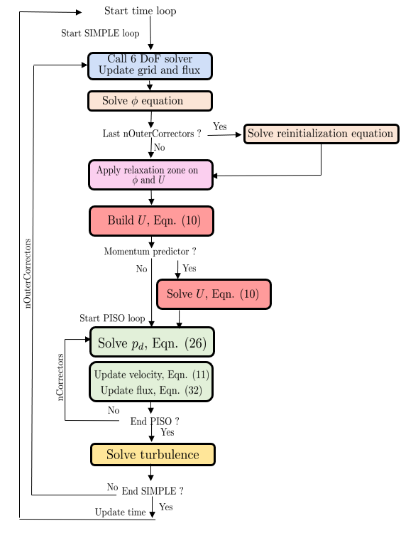
Figure 3: Segregated algorithm for LSFoam solver.

3 Test cases

3.1 The rising bubble test case, Hysing et al. [2007]

The rising bubble test case is a 2D benchmark from Hysing et al. [2007]. This test case has been simulated by many authors : Zuzio and Estivalezes [2011], Klostermann et al. [2013], Balcázar et al. [2016], Patel and Natarajan [2017], Gamet et al. [2020]. It consists of simulating a single rising bubble in a quiescent liquid. The domain sizes in the x and y directions are 1 m and 2 m. A bubble of diameter $D=0.5$ m is initially centered at coordinates (x,y)=(0.0, 0.5). Top and bottom boundaries are non-slipping walls, whereas lateral walls are slipping ones. Two configurations, TC1 and TC2 are simulated and resumed in table 1. The Reynolds number $R_{e}$, the Etvs number $E_{O}$ and the capillary number $C_{a}$ are defined as:

$$\begin{array}[]{ccc}R_{e}=\frac{\rho_{1}U_{g}D}{\mu_{1}}&\;\;\;\;E_{O}=\frac{\rho_{1}U_{g}^{2}D}{\sigma}&\;\;\;\;C_{a}=\frac{E_{O}}{R_{e}}\end{array}$$ (34)

Where $U_{g}=\sqrt{gD}$. Four levels of Cartesian grid refinements are studied : 32x64, 64x128, 128x256 and 256x512. Simulations are performed using an adaptive time step based on a maximal Courant number value of 0.05. The solver is set in PIMPLE (Issa [1986]) mode, and the number of loops depends on the residual of each iteration. The PIMPLE algorithm stops when the calculated residuals are lower than $\epsilon_{p_{d}}<10^{-5}$, $\epsilon_{\textbf{U}}<10^{-4}$ and $\epsilon_{\psi}<10^{-6}$. The convection term in the momentum equation is discretized with a second order upwind scheme (linearUpwind) and the dynamic pressure gradient is calculated using a least square method corrected at the interface (Ghost Fluid Method). Time advancement is achieved with the 2nd order backward scheme (backward). The reinitialization equation is solved 10 times at each time step with a reinitialization Courant number of 0.75. This procedure allows to fully recover the signed distance property of the level-set function. The characteristic length $\epsilon$ is chosen as $2\Delta z(\boldsymbol{x})$. The mass error is less than $10^{-3}$ %.

case	$\rho_{1}$	$\rho_{2}$	$\mu_{1}$	$\mu_{2}$	$g$	$\sigma$	$R_{e}$	$E_{O}$	$C_{a}$	$\frac{\rho_{1}}{\rho_{2}}$	$\frac{\mu_{1}}{\mu_{2}}$
TC1	1000	100	10	1	0.98	24.5	35	10	0.286	10	10
TC2	1000	1	10	0.1	0.98	1.96	35	125	3.571	1000	100

Table 1: TC1 and TC2: Physical properties and similarity parameters

Two quantities are used to compare the simulation results with the reference data of Hysing et al. [2007]: the position of the bubble center of mass (equation 35) and the bubble vertical velocity (equation 36).

$$\boldsymbol{X}_{c}=\frac{\int\alpha\boldsymbol{x}dx}{\int\alpha dx}$$ (35)

$$V_{y}=\frac{\int\alpha v_{y}dx}{\int\alpha dx}$$ (36)

Where $\alpha$ is the volume fraction as defined in equation 19. The bubble center of mass evolutions are presented in Figure 4 for each level of grid refinement. Overall results are in relatively good agreement with the data of Hysing et al. [2007], especially for the two finest grids. The rising velocity results are presented in Figure 5. As for the bubble center of mass, there is a good agreement between the presented results and the data of Hysing et al. [2007]. The results tend to be closer to the reference data with grid refinements. The numerical results can also be compared qualitatively by comparing the bubble shape for two test cases as presented in Figure 6.

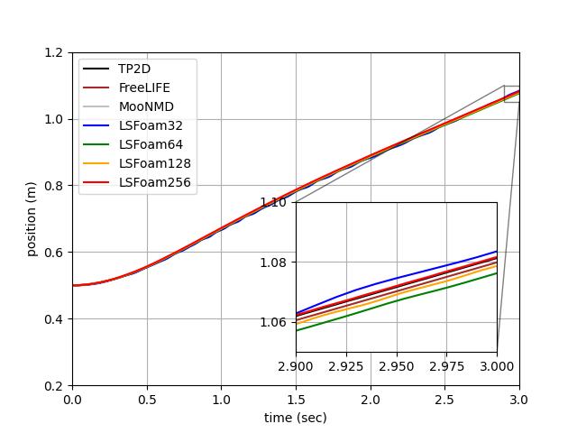
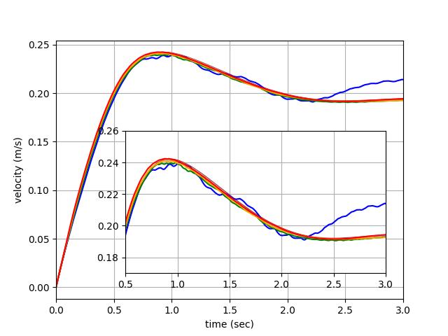
Figure 4: Case TC1 : Bubble center of mass coordinates and rising velocity comparison with data of Hysing et al. [2007] .

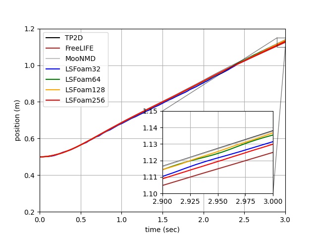
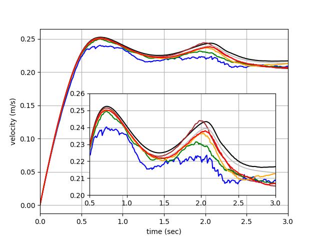
Figure 5: Case TC2 : Bubble center of mass coordinates and rising velocity comparison with data of Hysing et al. [2007] .

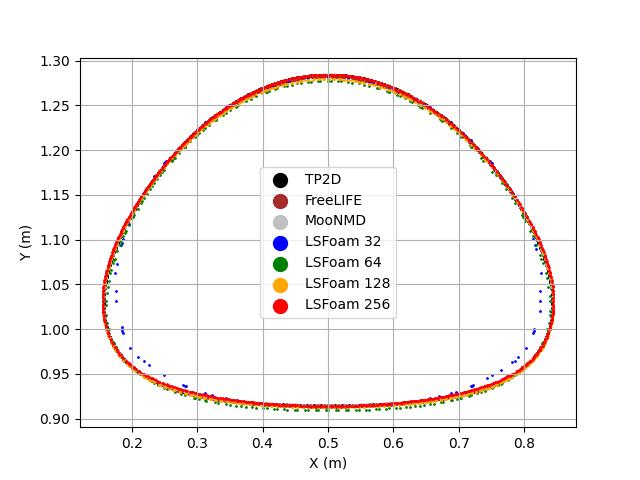
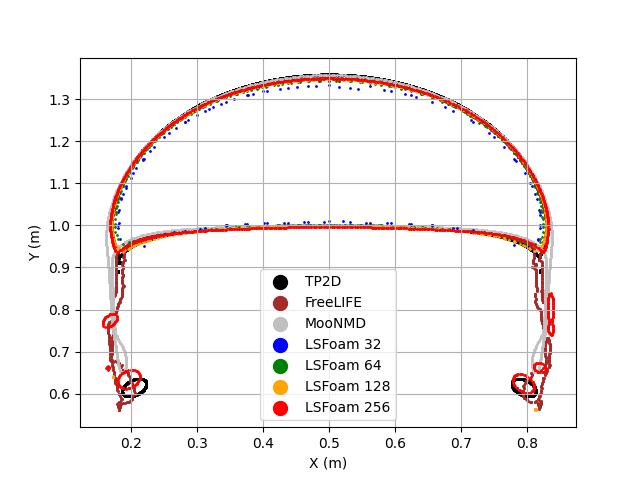
Figure 6: Case TC1 and TC2 : Bubble shape comparison with data of Hysing et al. [2007].

3.2 Rayleigh-Taylor instability, Puckett et al. [1997]

The Rayleigh-Taylor instability test case is a popular 2D numerical benchmark for complex multiphase flows. The problem has been initially proposed by Puckett et al. [1997] and simulated by many authors during the last two decades: Popinet and Zaleski [1999], Herrmann [2008], Sheu et al. [2009], Talat et al. [2018] or Kim and Park [2021]. The case consists in modeling two fluids with different density, $\rho_{1}=1.225$ and $\rho_{2}=0.1694kg/m^{3}$, but with the same viscosity $\mu=0.00313Pa.s$ in a rectangular domain of size 1 m x 4 m. The heavier fluid is positioned above the lighter one, and the interface is initially shaped with a sinusoidal perturbation of amplitude 0.05 m. The top and bottom boundaries are non-slipping walls, whereas the lateral ones are slipping walls. Four levels of Cartesian grid refinements are studied : 64x256, 128x512, 256x1024 and 512x2048. Simulations are performed using an adaptive time step based on a maximal Courant number value of 0.2. The numerical settings are identical to the rising bubble test cases. Results are presented in figures 7 and figure 8 for mesh sensitivity and comparison with reference data. The mushroom shape tends to converge with grid refinement. The comparison with reference results shows a medium level of agreement, except with the data of Sheu et al. [2009] where the results are closer. The mass variation relative error is below $10^{-4}$.

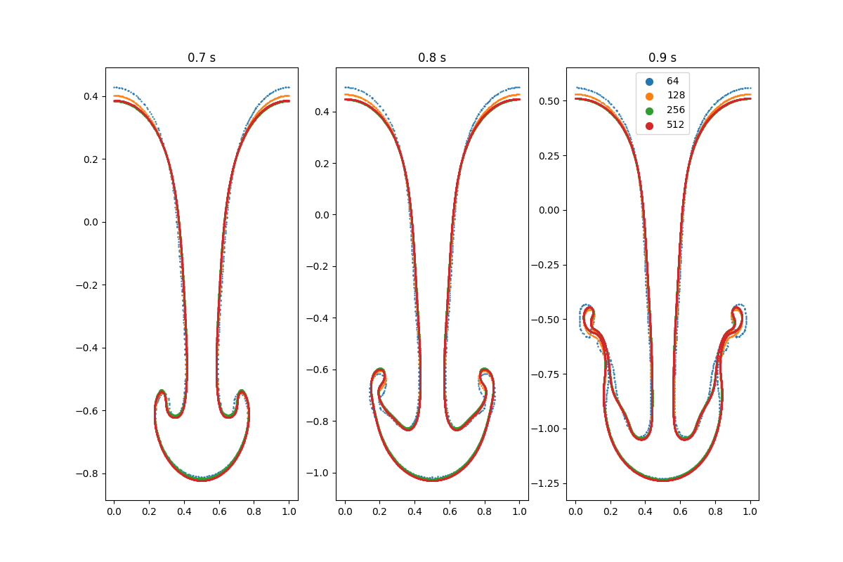
Figure 7: Rayleigh-Taylor instability. Shape comparison for mesh sensitivity results.

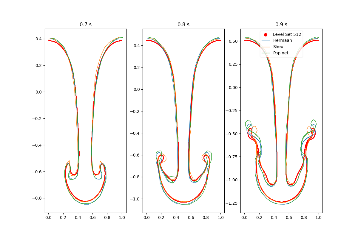
Figure 8: Rayleigh-Taylor instability. Shape comparison between finest grids and reference solutions.

3.3 Flow around an Ogee crest, Erpicum et al. [2018]

The flow around a scale model of an Ogee spillway crest is reproduced. The W2 Ogee spillway geometry is modeled with a design head $H_{d}$ of 10 cm (corresponding to case W2 of Peltier et al. [2018], Erpicum et al. [2018]) and have been built with the following equations from Hager [1987] and Imanian and Mohammadian [2019]:

$$\left(\frac{x}{H_{d}}+0.2418\right)^{2}+\left(\frac{z}{H_{d}}+0.1360\right)^{2}=0.04^{2}\;\text{for}\;-0.2818\leq\frac{x}{H_{d}}\leq-0.276\$$ (37)

$$\left(\frac{x}{H_{d}}+0.105\right)^{2}+\left(\frac{z}{H_{d}}+0.219\right)^{2}=0.2^{2}\;\text{for}\;-0.2276\leq\frac{x}{H_{d}}\leq-0.175$$ (38)

$$\left(\frac{x}{H_{d}}\right)^{2}+\left(\frac{z}{H_{d}}+0.5\right)^{2}=0.5^{2}\;\text{for}\;-0.175\leq\frac{x}{H_{d}}\leq 0$$ (39)

$$\frac{z}{H_{d}}=-0.5*\left(\frac{x}{H_{d}}\right)^{1.85}\;\text{for}\;\frac{x}{H_{d}}\geq 0$$ (40)

With x = 0 corresponding to the highest point of the Ogee spillway. The 2D numerical domain, illustrated in Figure 9, is composed of an upstream tank, the Ogee spillway, and a discharge zone. At the inlet, a Robin boundary condition is implemented, imposing the velocity of the water phase while applying a zero gradient condition for the air phase. The reference pressure is imposed at top through an atmospheric boundary condition. Zero gradient conditions are applied for the right patch while the remaining patches are of type wall. The mesh sensitivity study didn’t show significant variation in the results, thus, the results are presented for one unstructured grid generated with snappyHexMesh and composed of 200k cells. The turbulence is solved with the EARSM turbulence model of Hellsten [2005]. Regarding the numerical settings, the Euler scheme is used for time derivatives since only the steady-state is of interest. The convection terms are discretized with the 2nd order upwind scheme (linearUpwind) with a limited gradient (cellLimited Gauss linear 1), and the MUSCL scheme (van Leer [1979]) is used to discretize the Level-Set convective term. The gradients are discretized with the Gauss linear scheme, except for the pressure one, which is discretized with the least square scheme. The time step is fixed at 10 ms, and the PIMPLE algorithm stops when the calculated residuals are lower than $\epsilon_{p_{d}}<10^{-5}$. For such a flow, the head $H$ is defined by the water depth $h$ relative to the crest corrected y a kinetic energy term :

$$H=h+\frac{Q^{2}}{2gB^{2}(h+h_{uf})}$$ (41)

Where $Q$ is the discharge ($m^{3}/s$), $B$ the spillway width, and $h_{uf}$ the height of upstream face of the spillway. A sensitivity analysis on the water velocity at the inlet patch is performed for determining the discharge coefficient $C_{D}=\frac{Q}{B\sqrt{2gH^{3}}}$ relative to the head ratio $H/H_{d}$ and comparing to the experimental data of Erpicum et al. [2018]. The water level is initialized at the crest, and the water velocity is ramped during 5 sec. The simulations are conducted for a sufficient time (50 sec) to ensure a stabilized state. The discharge coefficient relative to head ratio is shown in Figure 10. The overall trend is in medium agreement with experimental data, and the discharge coefficient is underestimated. However, the flow separation near $H/H_{d}=5.5$ is well captured. The deviations from the experimental data are likely caused by turbulence and/or 3D effects. More detailed investigations are out of the scope of this study. It has to be noticed that no drift of the water level has been observed, showing that the present method, at least for this test case, is mass conservative.

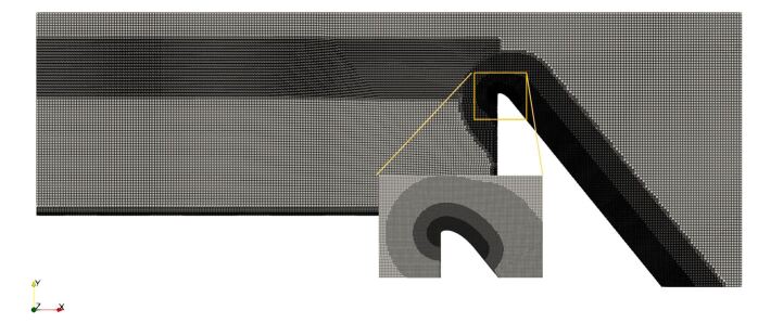
Figure 9: Ogee spillway simulation : Illustration of the two-dimensional mesh with 200k cells.

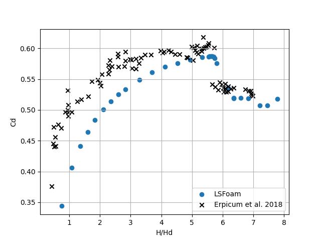
Figure 10: Discharge coefficients for different Head ratio with the W2 geometry.

3.4 Tridimensional dambreak simulation with a square cylinder obstacle, Gomez-Gesteira [2013]

This test case consists of simulating the fall of a water column and the impact of the generated wave on a square cylinder obstacle. Numerical facilities are described by Gomez-Gesteira [2013] and Ferro et al. [2022]. A water depth of 7.5 mm is initially placed beyond the gate (based on Vukcevic and Jasak [2014]). Force and fluid velocity in front of the obstacle measurements have been performed and are used for comparison with numerical results. The velocity probing point is located 146 mm in front of the obstacle, in the mid plane and 26 mm above the floor. Three mesh grids have been generated with blockMesh and are composed of : 130 k (coarse), 300 k (medium), and 3 M (fine) hexahedral cells. The finest one is illustrated Figure 11. Boundary conditions are wall types except for the top boundary, where an atmospheric boundary condition is simulated (totalPressure and pressureInletOutletVelocity). Simulations are carried out using an adaptive time step based on a maximal Courant number value of 0.25 for the interface and 0.5 for the rest. Turbulence is solved with the EARSM turbulence model of Hellsten [2005]. Convection terms are discretized with the 2nd order upwind scheme (linearUpwind) with a limited gradient (cellLimited Gauss linear 1). Gradients are discretized with the Gauss linear scheme, except the pressure one, which is discretize with the least square scheme. The MUSCL schemes (van Leer [1979]) is used to discretize the Level-Set convective term. Finally, the 2nd order backward scheme is chosen for time derivatives, and the PIMPLE algorithm stops when the calculated pressure residual is lower than $\epsilon_{p_{d}}<10^{-5}$. Force and velocity histories are presented in Figure 13. The offset in the first peak is also observed by Vukcevic and Jasak [2014] and Ye et al. [2020]. It may be caused by the fact that, experimentally, the gate can’t be instantly removed. Overall results are relatively similar and are in agreement with experimental data, even though the peaks are slightly overestimated. Regarding velocity measurements in front of the obstacle, the trend is properly captured. Free surface motions are detailed in Figure 14. The Figure 12 represents Level Set contours for the finest grid and illustrates that the Level Set distance property is well preserved. In this case, where the free surface motions are complex, the relative error of mass variation is inferior to 1%.

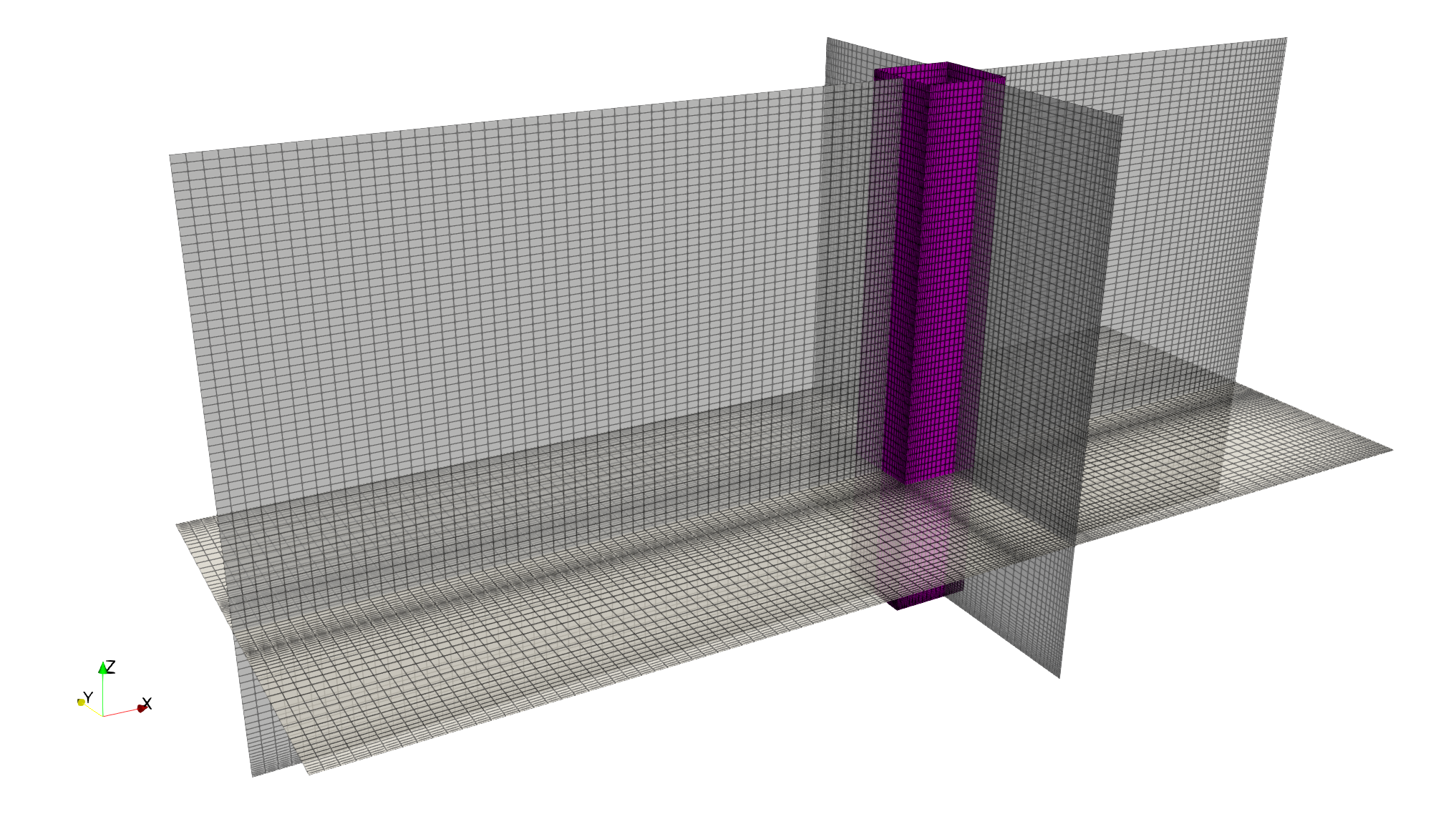
Figure 11: View of the finest non-uniform Cartesian grid built with blockMesh - 3 M cells. The square obstacle is colored in purple.

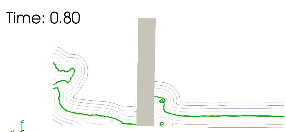
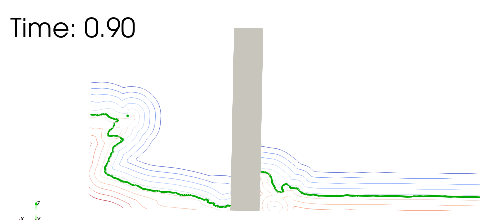
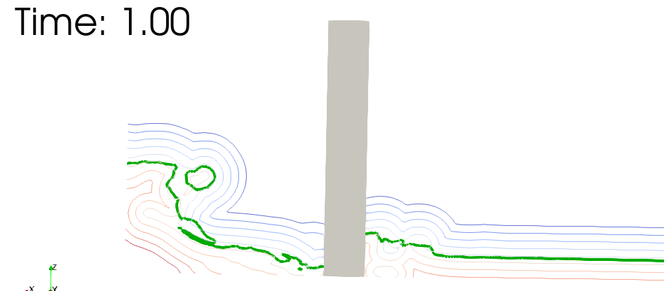
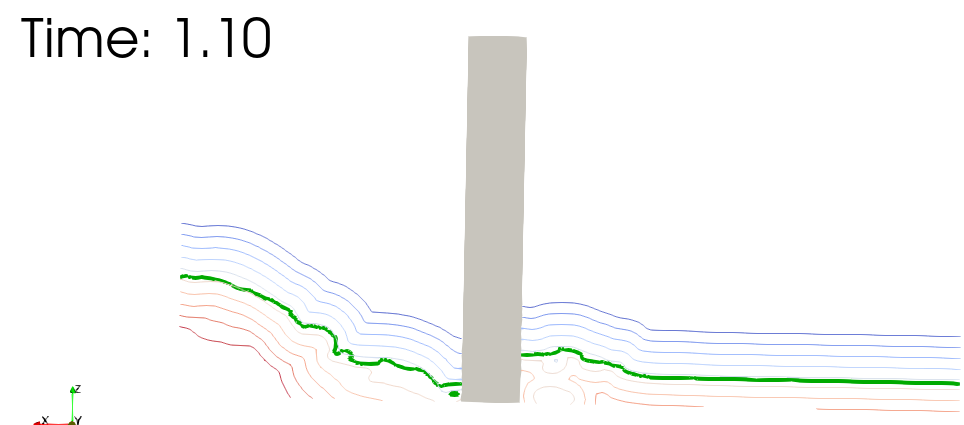
Figure 12: Level Set contours - from -0.1 to 0.1 - $\phi(\boldsymbol{x})=0$ in green.

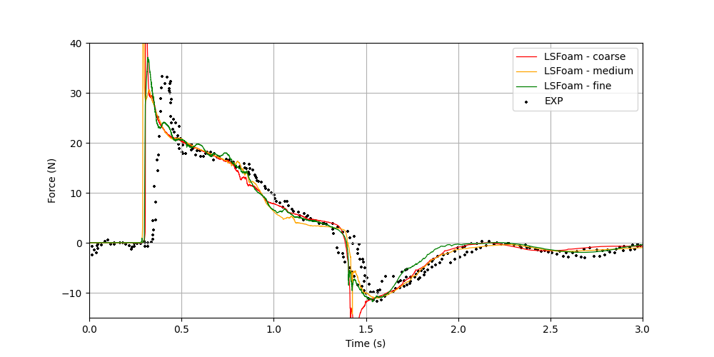
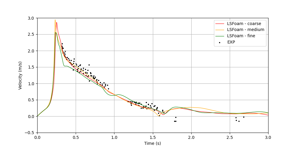
Figure 13: Force and velocities result and comparison for the 3 grids with experimental data Gomez-Gesteira [2013].

.

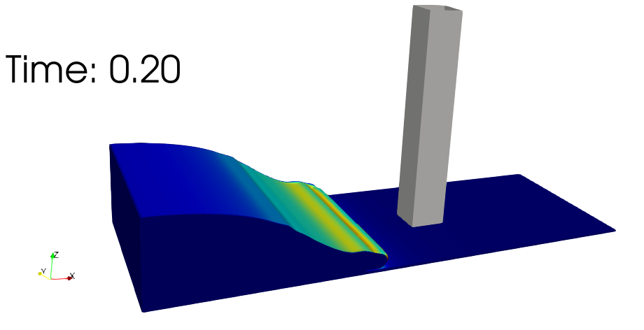
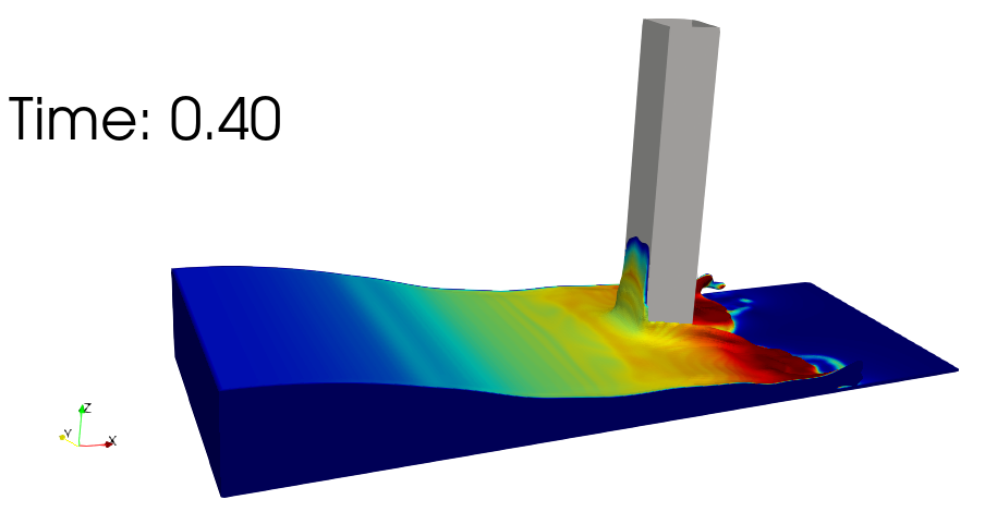
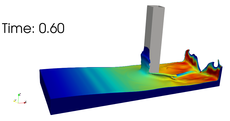
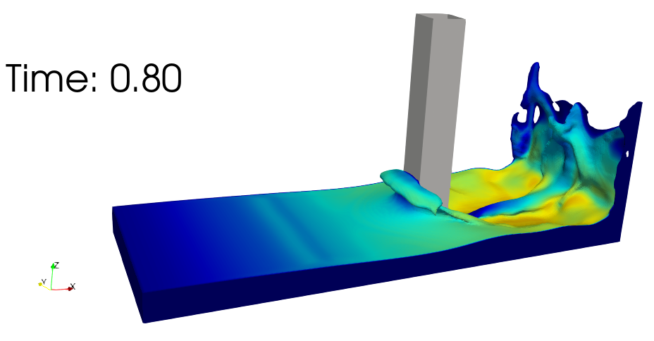
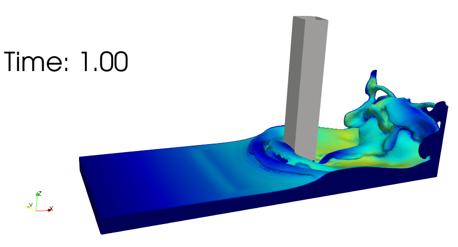
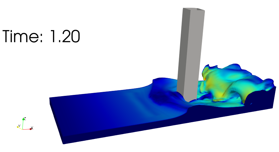
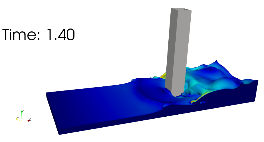
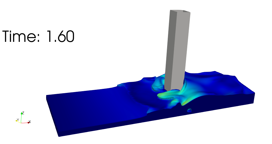
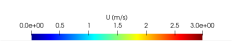
Figure 14: Free surface motions.

3.5 Gothenburg workshop, 2010, KVLCC2 steady resistance, Larsson et al. [2014]

The KVLCC2 (H and H [2001]) is a model scale ship. Its main particularities are detailed in Table 2. Test cases 1.b and 1.2a are parts of the 2010 Gothenburg workshop (Larsson et al. [2014]) and consist in simulating a towing tank test with a Froude number equal to 0.142 (1.047 m/s). The KVLCC2 test case is challenging for free surface methods as the maximum wave height is less than 1% of $L_{pp}.$ Numerical results are compared with resistance and wave elevation measurements. Simulations are carried out in the fixed ship reference frame with a symmetry hypothesis on the y = 0 plane. The air/water flow is imposed at the entrance of the computational box. A pressure reference is imposed on top through atmospheric boundary conditions. For bottom and lateral patches, a slip condition is used, while for outlet ones, zero gradient conditions are defined. Wall functions are used for the hull patch. Four levels of mesh refinement are generated with snappyHexMesh with respectively 1.7 M, 2.37 M , 3.2 M and 5.5 M cells (lately referred to coarse/grid 0, medium/grid 1, fine/grid 2 and vfine/grid 3). The average grid refinement ratio between grids, $r_{g}=1.2$ is calculated and used for the grid convergence study. The mesh is built using several refinement zones and illustrated on Figure 15. In the near-hull region, cells are refined in each direction within a rectangular box. Close to the free surface, cells are refined in the vertical direction. Moreover, in the Kelvin wake region, cells are also refined in longitudinal (Ox) and transversal (Oy) directions. Finally, 8 boundary layer cells are inflated with 100 % of cover layer rate. The time step has been fixed to 20 ms resulting in a maximum Courant number of 50 for the finest grid. The time discretization is achieved with first order Euler scheme because only steady-state results are of interest. The spatial discretization is identical to 3D dambreak simulation and the PIMPLE algorithm stops when the calculated pressure residual is lower than $\epsilon_{p_{d}}<10^{-5}$. An EARSM turbulence model Hellsten [2005] is used. The steady state drag coefficients are calculated and compared to experimental data for the 3 finest grids, as shown in Figure 16. Following Vukcevic [2016] guidelines, grid refinement study results and validation on grid 1, 2 and 3 are presented in Table 3. A relaxation zone is added to damp the free surface and velocity perturbations. The resistance coefficient relative errors are lower than 2%. Figure 17 represents the phase fraction and some contours $\phi(\boldsymbol{x})=constant$ illustrating that the Level Set function is well preserved. LSFoam wave patterns, presented on the top side of Figure 18, are reasonably matching the experimental data (bottom side of Figure 18). Regarding Figure 19, that represents the free surface elevations (z/Lpp for some planes y/Lpp = constant), LSFoam results fit the experimental data for planes y/Lpp= 0.09640 and y/Lpp = 0.1581. On the plane y/Lpp = 0.2993, free surface oscillations are slightly overestimated for the finest grid and probably caused by wave reflection due to the mesh transition outside the Kelvin triangle. Regarding mass conservation, for the finest grid, the relative error mass is below $10^{-5}$ showing the ability of the present method to maintain mass and hence the water level.

Designation	Prototype	TT model
Scale ratio	1	1/58
Speed (m/s)	7.9739	1.047
Froude number	0.142	0.142
Reynolds number	2.1 x $10^{9}$	4.6 x $10^{6}$
Length (m)	320	5.5172
Breadth (m)	58	1
Depth (m)	30	0.5172
Draft (m)	20.8	0.3586
Wetted surface area (m²)	27194	8038.8
Displacement (m3)	312.621	1.6023
Block coefficient	0.8098	0.8098

Table 2: KVLCC2 main particulars.

Figure 15: KVLCC2 mesh obtained with snappyHexMesh - very fine grid. 5.5 M cells.

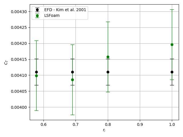
Figure 16: Force coefficient comparison between LSFoam and experimental data. The blue bars indicate the experimental uncertainty of 1 %. The green bars is the mesh uncertainty with a total height of $2U_{G}$.

Measurement Result	$C_{T}$
Experimental Result	0.00411
Experimental uncertainty (%)	1 %
Grid 1 solution	0.004158
Grid 2 solution	0.004086
Grid 3 solution	0.004099
Error grid 1	0.00004
Error grid 2	-0.00002
Error grid 3	-0.00001
Relative error grid 1 (%)	1.16 %
Relative error grid 2 (%)	-0.58 %
Relative error grid 3 (%)	-0.26 %
$R_{i}$	$-1<R_{i}<0$, oscillatory convergence
$U_{SN}$	0.01 %
$U_{G}$	1.3 %
$U_{v}$	0.01 %

Table 3: KVLCC2 validation and grid refinement study for the three finest grid.

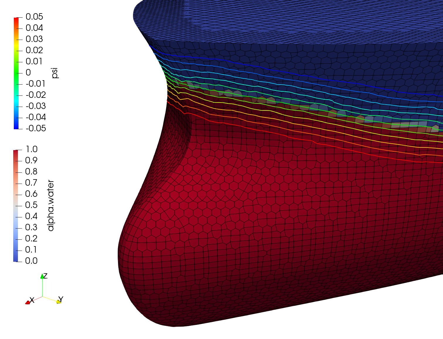
Figure 17: Illustration of hull phase fraction with $\phi(\boldsymbol{x})=$ -0.05 m to 0.05 m each 0.01 m.

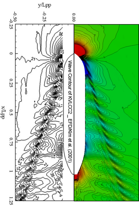
Figure 18: KVLCC2 wave pattern illustration - left EFD - right LSFoam finest grid.

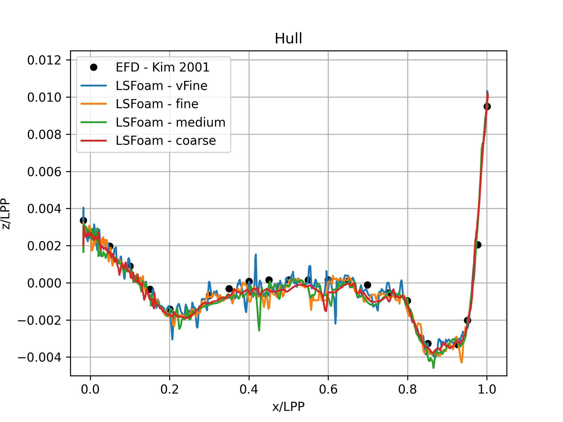
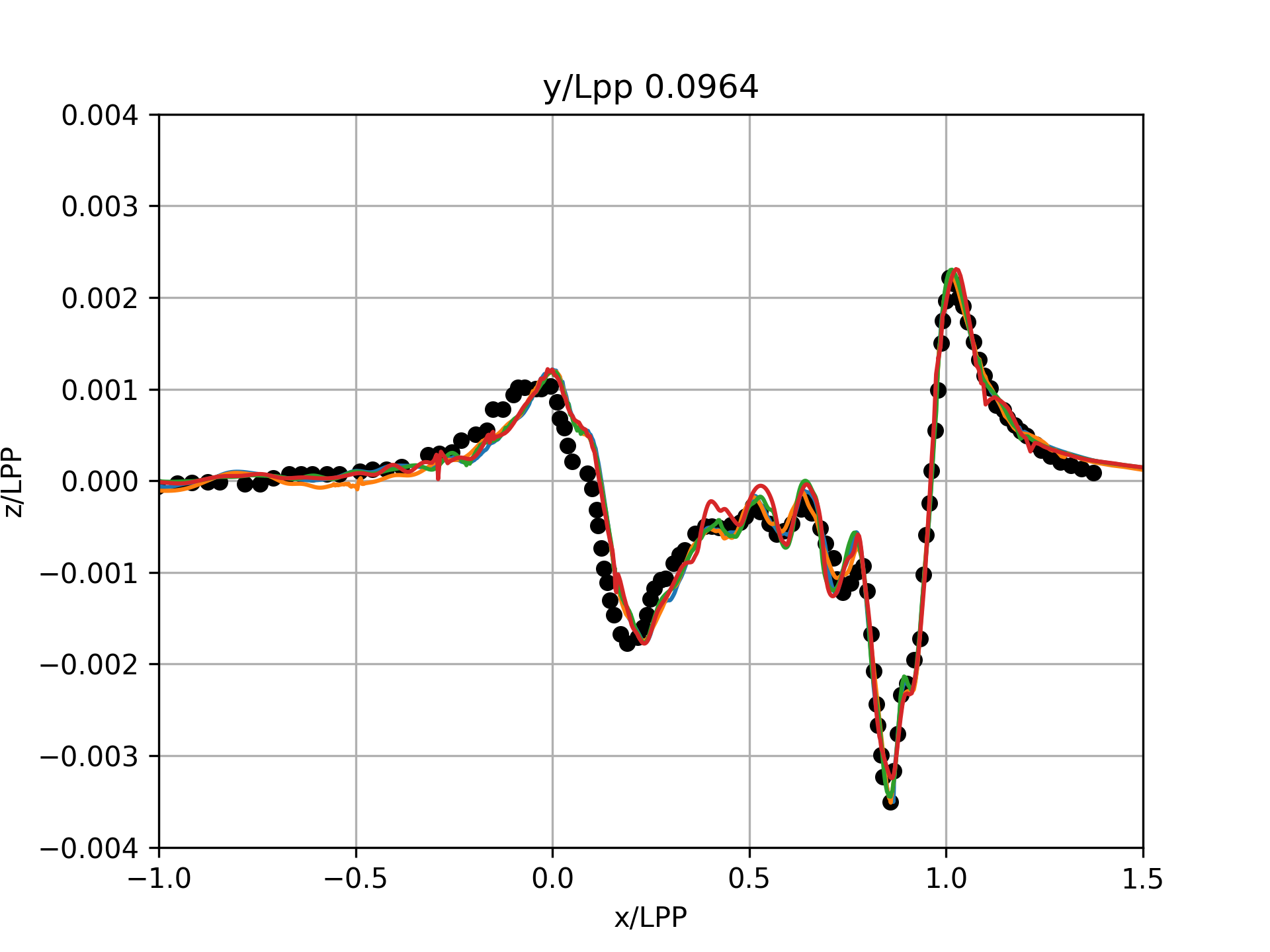
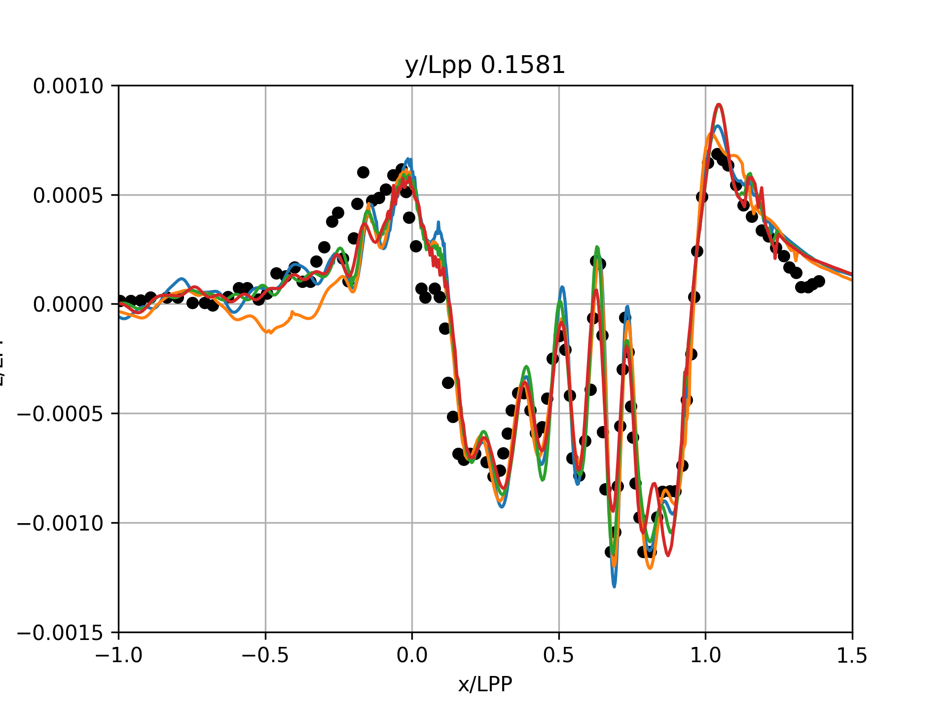
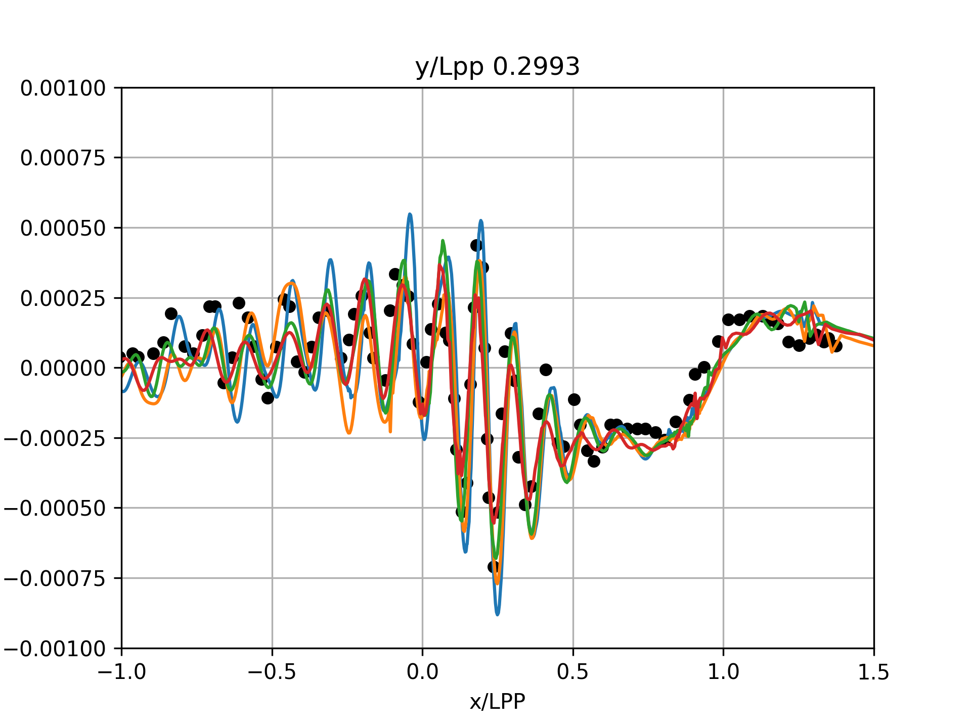
Figure 19: CFD free surface elevation (z/Lpp) comparison with experimental data on y/Lpp lines.

4 Conclusions

The Level Set algebraic-like approach (Sussman et al. [1994]) is based on a function $\phi$ being the signed distance to the interface. To capture interface motions, this function is advected in a flow field. Such a procedure will break its distance property and lead to unacceptable mass variations. To tackle these issues, the reinitialization Equation 5 from Sussman et al. [1994] is traditionally solved explicitly, but many practical limits remain : robustness, reinitialization frequency, number of iterations, mass variation, and polyhedral meshes. In this work, we propose to cover all these issues by :

• Adopting an implicit form of the reinitialization equation with LTS time advancement,

• Implementing an adaptive thickness size for sign and filtering functions,

• Enforcing the immobility of the interface during reinitialization iteration through the marking of anchoring cells.

For the pressure-velocity coupling, in a perspective to enhanced both accuracy and robustness, the solver takes advantage of the PIMPLE algorithm with a consistent momentum interpolation formulation Cubero and Fueyo [2007] and the GFM Fedkiw et al. [1999] for handling density discontinuities Vukčević et al. [2017]. With this Level-Set approach, the GFM is eased by the direct calculation of the distance to the interface.

The present approach has been coded in the OpenFOAM Weller et al. [1998] framework within a new solver, named LSFoam, and has been tested on five test cases covering different flow configurations: the rising bubble test case, Hysing et al. [2007], Rayleigh-Taylor instability simulations (Puckett et al. [1997]), Ogee spillway flow Erpicum et al. [2018], tridimensional dambreak simulation with a square cylinder obstacle Gomez-Gesteira [2013] and KVLCC2 steady resistance calculations (Larsson et al. [2014]). For the first two cases with surface tension dominated flow, the solver gave results very close to reference solutions. To challenge the method, non-uniform and unstructured grids have been used for the last 3 cases. For the Ogee spillway test, the method efficiently maintains the water level. The overall results are in medium agreement with the data of Erpicum et al. [2018] although the flow detachment is well predicted. Deviations in the discharge coefficient are observed but are likely caused by turbulence modeling and/or 2D assumption. For the dambreak simulation, the results are in good agreement with the experimental data. For ship resistance applications, the present method has shown excellent mass conservation properties as well as force calculations and wave patterns. Regarding mass losses, the conservation is excellent for all cases excepting for the 3D dambreak, where the motion of the free surface is very complex, although the mass error is limited to 1%. A potential solution could be to add a method to enforce mass conservations for such cases. The original approach of Sussman et al. [1994] with adequate enhancement is able to give overall excellent results for different flow configurations. The method is particularly promising for moderate free surface deformations typically encountered in marine and offshore applications.

5 Declaration of competing interests

The authors declare that they have no known competing financial.

References

- Balcázar et al. [2016] N. Balcázar, O. Lehmkuhl, L. Jofre, J. Rigola, and A. Oliva. A coupled volume-of-fluid/level-set method for simulation of two-phase flows on unstructured meshes. Computers and Fluids, 124:12–29, 2016. ISSN 0045-7930. doi: https://doi.org/10.1016/j.compfluid.2015.10.005. URL https://www.sciencedirect.com/science/article/pii/S0045793015003394. Special Issue for ICMMES-2014.
- Boris and Book [1997] J. P. Boris and D. L. Book. Flux-corrected transport. Journal of Computational Physics, 135(2):172–186, 1997. ISSN 0021-9991. doi: https://doi.org/10.1006/jcph.1997.5700. URL https://www.sciencedirect.com/science/article/pii/S0021999197957004.
- Cubero and Fueyo [2007] A. Cubero and N. Fueyo. A compact momentum interpolation procedure for unsteady flows and relaxation. Numerical Heat Transfer, Part B: Fundamentals, 52(6):507–529, 2007. doi: 10.1080/10407790701563334. URL https://doi.org/10.1080/10407790701563334.
- DeBar [1974] R. B. DeBar. Fundamentals of the kraken code. [eulerian hydrodynamics code for compressible nonviscous flow of several fluids in two-dimensional (axially symmetric) region]. 3 1974. doi: 10.2172/7227630. URL https://www.osti.gov/biblio/7227630.
- Erpicum et al. [2018] S. Erpicum, B. Blancher, J. Vermeulen, Y. Peltier, P. Archambeau, B. Dewals, and M. Pirotton. Experimental study of ogee crested weir operation above the design head and influence of the upstream quadrant geometry. 2018.
- Fedkiw et al. [1999] R. P. Fedkiw, T. Aslam, and S. Xu. The ghost fluid method for deflagration and detonation discontinuities. Journal of Computational Physics, 154(2), 9 1999. ISSN 0021-9991. doi: 10.1006/jcph.1999.6320. URL https://www.osti.gov/biblio/20000635.
- Ferro et al. [2022] P. Ferro, P. Landel, M. Pescheux, and S. Guillot. Development of a free surface flow solver using the ghost fluid method on openfoam. Ocean Engineering, 253:111236, 2022. ISSN 0029-8018. doi: https://doi.org/10.1016/j.oceaneng.2022.111236. URL https://www.sciencedirect.com/science/article/pii/S0029801822006321.
- Gamet et al. [2020] L. Gamet, M. Scala, J. Roenby, H. Scheufler, and J.-L. Pierson. Validation of volume-of-fluid openfoam® isoadvector solvers using single bubble benchmarks. Computers and Fluids, 213:104722, 2020. ISSN 0045-7930. doi: https://doi.org/10.1016/j.compfluid.2020.104722. URL https://www.sciencedirect.com/science/article/pii/S0045793020302929.
- Gomez-Gesteira [2013] Gomez-Gesteira. Spheric sph benchmark test cases: Test 1-force exerted by a schematic 3d dam break on a square cylinder. 2013.
- Gu et al. [2018] Z. Gu, H. Wen, C. Yu, and T. W. Sheu. Interface-preserving level set method for simulating dam-break flows. Journal of Computational Physics, 374:249–280, 2018. ISSN 0021-9991. doi: https://doi.org/10.1016/j.jcp.2018.07.057. URL https://www.sciencedirect.com/science/article/pii/S0021999118305205.
- Gärtner et al. [2020] J. W. Gärtner, A. Kronenburg, and T. Martin. Efficient weno library for openfoam. SoftwareX, 12:100611, 2020. ISSN 2352-7110. doi: https://doi.org/10.1016/j.softx.2020.100611. URL https://www.sciencedirect.com/science/article/pii/S2352711020303241.
- H and H [2001] K. W. J. V. S. H and K. D. H. Measurement of flows around modern commercial ship models. Experiments in Fluids, 31, Nov 2001. doi: 10.1007/s003480100332. URL https://doi.org/10.1007/s003480100332.
- Hager [1987] W. H. Hager. Continuous crest profile for standard spillway. Journal of Hydraulic Engineering, 113(11):1453–1457, 1987. doi: 10.1061/(ASCE)0733-9429(1987)113:11(1453). URL https://ascelibrary.org/doi/abs/10.1061/%28ASCE%290733-9429%281987%29113%3A11%281453%29.
- Haghshenas et al. [2019] M. Haghshenas, J. A. Wilson, and R. Kumar. Finite volume ghost fluid method implementation of interfacial forces in piso loop. Journal of Computational Physics, 376:20–27, 2019. ISSN 0021-9991. doi: https://doi.org/10.1016/j.jcp.2018.09.025. URL https://www.sciencedirect.com/science/article/pii/S0021999118306259.
- Hartmann et al. [2010] D. Hartmann, M. Meinke, and W. Schröder. The constrained reinitialization equation for level set methods. Journal of Computational Physics, 229(5):1514–1535, 2010. ISSN 0021-9991. doi: https://doi.org/10.1016/j.jcp.2009.10.042. URL https://www.sciencedirect.com/science/article/pii/S0021999109006032.
- Hellsten [2005] A. Hellsten. New advanced k-w turbulence model for high-lift aerodynamics. AIAA Journal, 43(9):1857–1869, 2005. doi: 10.2514/1.13754. URL https://doi.org/10.2514/1.13754.
- Henri [2021] F. Henri. Améliorations des méthodes Level Set pour l’impact de goutte de pluie. Theses, Université de Bordeaux, Dec. 2021. URL https://theses.hal.science/tel-03527520.
- Herrmann [2008] M. Herrmann. A balanced force refined level set grid method for two-phase flows on unstructured flow solver grids. Journal of Computational Physics, 227(4):2674–2706, 2008. ISSN 0021-9991. doi: https://doi.org/10.1016/j.jcp.2007.11.002. URL https://www.sciencedirect.com/science/article/pii/S0021999107004998.
- Hirt and Nichols [1981] C. Hirt and B. Nichols. Volume of fluid (vof) method for the dynamics of free boundaries. Journal of Computational Physics, 39(1):201–225, 1981. ISSN 0021-9991. doi: https://doi.org/10.1016/0021-9991(81)90145-5. URL https://www.sciencedirect.com/science/article/pii/0021999181901455.
- Hong et al. [2007] J.-M. Hong, T. Shinar, M. joo Kang, and R. Fedkiw. On boundary condition capturing for multiphase interfaces. Journal of Scientific Computing, 31:99–125, 2007.
- Huang et al. [2007] J. Huang, P. M. Carrica, and F. Stern. Coupled ghost fluid/two-phase level set method for curvilinear body-fitted grids. International Journal for Numerical Methods in Fluids, 55(9):867–897, 2007. doi: https://doi.org/10.1002/fld.1499. URL https://onlinelibrary.wiley.com/doi/abs/10.1002/fld.1499.
- Hysing et al. [2007] S. Hysing, S. Turek, D. Kuzmin, N. Parolini, E. Burman, S. Ganesan, and L. Tobiska. Proposal for quantitative benchmark computations of bubble dynamics. Ergebnisberichte des Instituts für Angewandte Mathematik, Nummer 351, Fakultät für Mathematik, TU Dortmund, 2007.
- Imanian and Mohammadian [2019] H. Imanian and A. Mohammadian. Numerical simulation of flow over ogee crested spillways under high hydraulic head ratio. Engineering Applications of Computational Fluid Mechanics, 13(1):983–1000, 2019. doi: 10.1080/19942060.2019.1661014. URL https://doi.org/10.1080/19942060.2019.1661014.
- Issa [1986] R. Issa. Solution of the implicitly discretised fluid flow equations by operator-splitting. Journal of Computational Physics, 62(1):40–65, 1986. ISSN 0021-9991. doi: https://doi.org/10.1016/0021-9991(86)90099-9. URL https://www.sciencedirect.com/science/article/pii/0021999186900999.
- Jacobsen et al. [2012] N. G. Jacobsen, D. R. Fuhrman, and J. Fredsøe. A wave generation toolbox for the open-source cfd library: Openfoam®. International Journal for Numerical Methods in Fluids, 70(9):1073–1088, 2012. doi: https://doi.org/10.1002/fld.2726. URL https://onlinelibrary.wiley.com/doi/abs/10.1002/fld.2726.
- Jasak [1996] H. Jasak. Error Analysis and Estimation for the Finite Volume Method with Applications to Fluid Flows. PhD thesis, 1996.
- Johansson [2011] N. Johansson. Implementation of a standard level set method for incompressible two-phase flow simulations. 2011. URL https://api.semanticscholar.org/CorpusID:118330967.
- Kang et al. [2000] M. Kang, R. P. Fedkiw, and X.-D. Liu. A boundary condition capturing method for multiphase incompressible flow. J. Sci. Comput., 15(3):323–360, sep 2000. ISSN 0885-7474. doi: 10.1023/A:1011178417620. URL https://doi.org/10.1023/A:1011178417620.
- Khosronejad et al. [2019] A. Khosronejad, M. G. Arabi, D. Angelidis, E. Bagherizadeh, K. Flora, and A. Farhadzadeh. Comparative hydrodynamic study of rigid-lid and level-set methods for les of open-channel flow. Journal of Hydraulic Engineering, 145(1):04018077, 2019. doi: 10.1061/(ASCE)HY.1943-7900.0001546. URL https://ascelibrary.org/doi/abs/10.1061/%28ASCE%29HY.1943-7900.0001546.
- Kim and Park [2021] H. Kim and S. Park. Coupled level-set and volume of fluid (clsvof) solver for air lubrication method of a flat plate. Journal of Marine Science and Engineering, 9(2), 2021. ISSN 2077-1312. doi: 10.3390/jmse9020231. URL https://www.mdpi.com/2077-1312/9/2/231.
- Klostermann et al. [2013] J. Klostermann, K. Schaake, and R. Schwarze. Numerical simulation of a single rising bubble by vof with surface compression. International Journal for Numerical Methods in Fluids, 71(8):960–982, 2013. doi: https://doi.org/10.1002/fld.3692. URL https://onlinelibrary.wiley.com/doi/abs/10.1002/fld.3692.
- Lalanne et al. [2015] B. Lalanne, L. R. Villegas, S. Tanguy, and F. Risso. On the computation of viscous terms for incompressible two-phase flows with level set/ghost fluid method. Journal of Computational Physics, 301:289–307, 2015. ISSN 0021-9991. doi: https://doi.org/10.1016/j.jcp.2015.08.036. URL https://www.sciencedirect.com/science/article/pii/S002199911500563X.
- Larsson et al. [2014] L. Larsson, F. Stern, and M. Visonneau. Numerical ship hydrodynamics. An assessment of the 6th Gothenburg 2010 workshop. Springer Netherlands, 1 edition, Dec. 2014. doi: 10.1007/978-94-007-7189-5.
- Leroyer et al. [2011] A. Leroyer, J. Wackers, P. Queutey, and E. Guilmineau. Numerical strategies to speed up cfd computations with free surface—application to the dynamic equilibrium of hulls. Ocean Engineering, 38(17):2070–2076, 2011. ISSN 0029-8018. doi: https://doi.org/10.1016/j.oceaneng.2011.09.006. URL https://www.sciencedirect.com/science/article/pii/S0029801811002009.
- Liu et al. [1994] X.-D. Liu, S. Osher, and T. Chan. Weighted essentially non-oscillatory schemes. Journal of Computational Physics, 115(1):200–212, 1994. ISSN 0021-9991. doi: https://doi.org/10.1006/jcph.1994.1187. URL https://www.sciencedirect.com/science/article/pii/S0021999184711879.
- Martin and Shevchuk [2018] T. Martin and I. Shevchuk. Implementation and validation of semi-implicit weno schemes using openfoam®. Computation, 6(1), 2018. ISSN 2079-3197. doi: 10.3390/computation6010006. URL https://www.mdpi.com/2079-3197/6/1/6.
- Muzaferija [1998] S. Muzaferija. A two-fluid navier-stokes solver to simulate water entry. Proceeding of the 22nd symposium of naval hydrodynamics. Washington, DC, 1998, 1998. URL https://ci.nii.ac.jp/naid/10019844096/en/.
- Osher and Fedkiw [2003] S. J. Osher and R. Fedkiw. Level set methods and dynamic implicit surfaces., volume 153 of Applied mathematical sciences. Springer, 2003. ISBN 0387954821.
- Park et al. [2005] I. R. Park, S. H. Van, J. Kim, and K. J. Kang. Level-set simulation of viscous free surface flow around a commercial hull form. 2005. URL https://api.semanticscholar.org/CorpusID:53370150.
- Patankar and Spalding [1972] S. Patankar and D. Spalding. A calculation procedure for heat, mass and momentum transfer in three-dimensional parabolic flows. International Journal of Heat and Mass Transfer, 15(10):1787–1806, 1972. ISSN 0017-9310. doi: https://doi.org/10.1016/0017-9310(72)90054-3. URL https://www.sciencedirect.com/science/article/pii/0017931072900543.
- Patel and Natarajan [2017] J. K. Patel and G. Natarajan. A novel consistent and well-balanced algorithm for simulations of multiphase flows on unstructured grids. Journal of Computational Physics, 350:207–236, Dec. 2017. doi: 10.1016/j.jcp.2017.08.047.
- Peltier et al. [2018] Y. Peltier, B. Dewals, P. Archambeau, M. Pirotton, and S. Erpicum. Pressure and velocity on an ogee spillway crest operating at high head ratio: Experimental measurements and validation. Journal of Hydro-environment Research, 19:128–136, 2018. ISSN 1570-6443. doi: https://doi.org/10.1016/j.jher.2017.03.002. URL https://www.sciencedirect.com/science/article/pii/S1570644316301757.
- Popinet and Zaleski [1999] S. Popinet and S. Zaleski. A front-tracking algorithm for accurate representation of surface tension. International Journal for Numerical Methods in Fluids, 30(6):775–793, 1999. URL https://hal.archives-ouvertes.fr/hal-01445441.
- Puckett et al. [1997] E. G. Puckett, A. S. Almgren, J. B. Bell, D. L. Marcus, and W. J. Rider. A high-order projection method for tracking fluid interfaces in variable density incompressible flows. Journal of Computational Physics, 130(2):269–282, 1997. ISSN 0021-9991. URL https://www.sciencedirect.com/science/article/pii/S0021999196955904.
- Rhie and Chow [1983] C. M. Rhie and W. L. Chow. Numerical study of the turbulent flow past an airfoil with trailing edge separation. AIAA Journal, 21(11):1525–1532, 1983. doi: 10.2514/3.8284. URL https://doi.org/10.2514/3.8284.
- Roenby et al. [2016] J. Roenby, H. Bredmose, and H. Jasak. A computational method for sharp interface advection. Royal Society Open Science, 3(11):160405, 2016. doi: 10.1098/rsos.160405. URL https://royalsocietypublishing.org/doi/abs/10.1098/rsos.160405.
- Rusche [2002] H. Rusche. Computational Fluid Dynamics of Dispersed Two-Phase Flows at High Phase Fractions. PhD thesis, Imperial College, London, 2002. URL http://powerlab.fsb.hr/ped/kturbo/OpenFOAM/docs/HenrikRuschePhD2002.pdf.
- Russo and Smereka [2000] G. Russo and P. Smereka. A Remark on Computing Distance Functions. Journal of Computational Physics, 163(1):51–67, Sept. 2000. doi: 10.1006/jcph.2000.6553.
- Sheu et al. [2009] T. W. Sheu, C. Yu, and P. Chiu. Development of a dispersively accurate conservative level set scheme for capturing interface in two-phase flows. Journal of Computational Physics, 228(3):661–686, 2009. ISSN 0021-9991. doi: https://doi.org/10.1016/j.jcp.2008.09.032. URL https://www.sciencedirect.com/science/article/pii/S0021999108005007.
- Sun et al. [2010] M. Sun, Z. Wang, and X.-S. Bai. Assessment and modification of sub-cell-fix method for re-initialization of level-set distance function. International Journal for Numerical Methods in Fluids, 62(2):211–236, 2010. ISSN 1097-0363. doi: 10.1002/fld.2204.
- Sussman et al. [1994] M. Sussman, P. Smereka, and S. Osher. A level set approach for computing solutions to incompressible two-phase flow. Journal of Computational Physics, 114(1):146–159, 1994. ISSN 0021-9991. doi: https://doi.org/10.1006/jcph.1994.1155.
- Sussman et al. [1998] M. Sussman, E. Fatemi, P. Smereka, and S. Osher. An improved level set method for incompressible two-phase flows. Computers and Fluids, 27(5):663–680, 1998. ISSN 0045-7930. doi: https://doi.org/10.1016/S0045-7930(97)00053-4. URL https://www.sciencedirect.com/science/article/pii/S0045793097000534.
- Talat et al. [2018] N. Talat, B. Mavrič, V. Hatić, S. Bajt, and B. Šarler. Phase field simulation of rayleigh–taylor instability with a meshless method. Engineering Analysis with Boundary Elements, 87:78–89, 2018. ISSN 0955-7997. doi: https://doi.org/10.1016/j.enganabound.2017.11.015. URL https://www.sciencedirect.com/science/article/pii/S0955799717304009.
- Titarev and Toro [2004] V. Titarev and E. Toro. Finite-volume weno schemes for three-dimensional conservation laws. Journal of Computational Physics, 201(1):238–260, 2004. ISSN 0021-9991. doi: https://doi.org/10.1016/j.jcp.2004.05.015. URL https://www.sciencedirect.com/science/article/pii/S0021999104002281.
- Trujillo [2021] M. F. Trujillo. Reexamining the one-fluid formulation for two-phase flows. International Journal of Multiphase Flow, 141:103672, 2021. ISSN 0301-9322. doi: https://doi.org/10.1016/j.ijmultiphaseflow.2021.103672. URL https://www.sciencedirect.com/science/article/pii/S0301932221001208.
- van Leer [1979] B. van Leer. Towards the ultimate conservative difference scheme. v. a second-order sequel to godunov’s method. Journal of Computational Physics, 32(1):101–136, 1979. ISSN 0021-9991. doi: https://doi.org/10.1016/0021-9991(79)90145-1. URL https://www.sciencedirect.com/science/article/pii/0021999179901451.
- Vukcevic [2016] V. Vukcevic. Numerical Modelling of Coupled Potential and Viscous Flow for Marine Applications. PhD thesis, 11 2016.
- Vukcevic and Jasak [2014] V. Vukcevic and H. Jasak. A conservative level set method for interface capturing in two-phase flows. 2014.
- Vukčević et al. [2017] V. Vukčević, H. Jasak, and I. Gatin. Implementation of the ghost fluid method for free surface flows in polyhedral finite volume framework. Computers and Fluids, 153:1–19, 2017. ISSN 0045-7930. doi: https://doi.org/10.1016/j.compfluid.2017.05.003. URL https://www.sciencedirect.com/science/article/pii/S0045793017301640.
- Weller et al. [1998] H. G. Weller, G. Tabor, H. Jasak, and C. Fureby. A tensorial approach to computational continuum mechanics using object-oriented techniques. Computers in Physics, 12(6):620–631, 1998. doi: 10.1063/1.168744. URL https://aip.scitation.org/doi/abs/10.1063/1.168744.
- Yamamoto et al. [2017] T. Yamamoto, Y. Okano, and S. Dost. Validation of the s-clsvof method with the density-scaled balanced continuum surface force model in multiphase systems coupled with thermocapillary flows. International Journal for Numerical Methods in Fluids, 83(3):223–244, 2017. doi: https://doi.org/10.1002/fld.4267. URL https://onlinelibrary.wiley.com/doi/abs/10.1002/fld.4267.
- Ye et al. [2020] H. Ye, Y. Chen, and K. Maki. A discrete-forcing immersed boundary method for moving bodies in air–water two-phase flows. Journal of Marine Science and Engineering, 8(10), 2020. ISSN 2077-1312. doi: 10.3390/jmse8100809. URL https://www.mdpi.com/2077-1312/8/10/809.
- Zuzio and Estivalezes [2011] D. Zuzio and J. Estivalezes. An efficient block parallel amr method for two phase interfacial flow simulations. Computers and Fluids, 44(1):339–357, 2011. doi: 10.1016/j.compfluid.2011.01.035.