Data Fusion for Heterogeneous Treatment Effect Estimation with Multi-Task Gaussian Processes

Abstract

Bridging the gap between internal and external validity is crucial for heterogeneous treatment effect estimation. Randomised controlled trials (RCTs), favoured for their internal validity due to randomisation, often encounter challenges in generalising findings due to strict eligibility criteria. Observational studies on the other hand, provide external validity advantages through larger and more representative samples but suffer from compromised internal validity due to unmeasured confounding. Motivated by these complementary characteristics, we propose a novel Bayesian nonparametric approach leveraging multi-task Gaussian processes to integrate data from both RCTs and observational studies. In particular, we introduce a parameter which controls the degree of borrowing between the datasets and prevents the observational dataset from dominating the estimation. The value of the parameter can be either user-set or chosen through a data-adaptive procedure. Our approach outperforms other methods in point predictions across the covariate support of the observational study, and furthermore provides a calibrated measure of uncertainty for the estimated treatment effects, which is crucial when extrapolating. We demonstrate the robust performance of our approach in diverse scenarios through multiple simulation studies and a real-world education randomised trial.

1 Introduction

Treatment effect estimation is an important task in many applications, including medicine, epidemiology, and the social sciences. The goal is to quantify the expected impact of a particular intervention in a given target population. For example, in medicine, one may seek to estimate the expected benefit or harm from taking a particular drug relative to placebo for a patient with a certain disease.

The Average Treatment Effect (ATE) from a study is often used as evidence for whether a particular intervention should be applied to an individual or unit in a given target population. The reliability of this evidence rests on two key assumptions. Firstly, the study population is assumed to be sufficiently similar to the target population, so that an estimate of the treatment effect is applicable to the target population in which the intervention under investigation will eventually be applied. Secondly, the average treatment effect is assumed to be close to an individual’s treatment effect.

This second assumption of homogeneity across individuals is often violated: the effect of an intervention within a population may vary systematically with respect to a particular covariate or combination of covariates. Returning to our medical example, a drug may have different effects for an individual as a function of their age or sex. In these cases, understanding the heterogeneity of treatment effects is critical to ensure that appropriate decisions are taken for all individuals, not just those who are similar to the average or belong to pre-specified subgroups that poorly reflect heterogeneity within the population (Brantner et al., 2023).

Whether the results of a study are relied upon for a particular decision or policy also depends on the statistical significance of the corresponding estimates. A proposed intervention with an estimated positive treatment effect may not be adopted if statistical variability indicates that this estimate is not significantly away from zero. Thus, an appropriate characterisation of the uncertainty of an estimate is also required. While this is reasonably straightforward in the computation of average treatment effects, uncertainty quantification for heterogeneous treatment effects is more challenging, especially when making inferences about individuals not represented in the randomised controlled trial (RCT), where classical methods rely heavily on extrapolation without proper variance inflation to reflect uncertainty (Degtiar and Rose, 2023).

The gold standard for treatment effect estimation remains the RCT. The random allocation of treatment to individuals in the study guards against the effect of confounding, assuming perfect compliance with allocated treatment. As a result, under a few additional assumptions, the difference in average outcomes between individuals in the treatment and control arms is unbiased for the average treatment effect in the study population.

There are, however, drawbacks to the use of RCTs (Frieden, 2017). They are typically expensive to carry out, and sample sizes can be limited as a result. While they may be powered enough to detect the main effect, they are typically underpowered for subgroup effects. Further, the study population may not be representative of the target population. This can be for a variety of reasons such as inclusion/exclusion criteria of individuals into the study (either on statistical, practical, or ethical grounds), or selection bias of individuals into the study; for instance, there may be differential acceptance to “invitation to participate" from eligible candidates according to, for example, socioeconomic status, educational levels or ethnicity (National Academies of Sciences, Engineering, and Medicine, 2022).

Observational, or ‘real-world’ studies, provide an alternative source of data for treatment effect estimation. In contrast to RCTs, they generally benefit from larger sample sizes and tend to be more representative of the target population. However, a number of assumptions must be made to ensure the validity of treatment effect estimations from observational data. In particular, one must assume that there are no unmeasured confounders - hidden variables that affect both the outcome of interest and the treatment allocation. While it may be possible to adjust for the effect of observed confounders, there is no way to mitigate the effect of unmeasured confounding without making strong assumptions about the nature of confounding.

The complementary nature of RCT and observational data indicates the potential benefits from combining the two sources to obtain better heterogeneous treatment effect estimates. Such data fusion approaches have received increased interest in recent years, and a range of methods have been developed to integrate information from multiple sources of data, including a limited number of applications to causal inference problems (see Colnet et al. (2023) for a recent review). These typically rely on strong, untestable assumptions about the structure of the confounding effect and, moreover, are not able to provide uncertainty quantification around the point estimates of heterogeneous treatment effects.

In this paper, we introduce a Bayesian non-parametric approach to obtain estimates of heterogeneous treatment effects for the target population, with uncertainty quantification. Our approach is based on multi-output Gaussian Processes, where the limited RCT observations are used to correct the confounding effect on the observational data. Our key contributions are as follows:

• We introduce an Intrinsic Coregionalization Model (ICM) for heteregeneous treatment effect estimation, which we call Causal-ICM. Causal-ICM is a multi-task Gaussian process (GP) model that enables accurate treatment effect estimation within and outside of the support of the RCT and calibrated uncertainty quantification of treatment effect estimates across the support of the target population, without relying on strong assumptions on the structure of the hidden confounding effect.

• Causal-ICM has a straightforward interpretation, relying on a key hyperparameter that quantifies the measure of trust in the quality of the observational data, and can be tuned data-adaptively. We provide theory to demonstrate that the ICM is robust against the dominating nature of a large observational dataset.

• We demonstrate excellent empirical performance in simulations and a real dataset relative to other benchmarks for both point estimation and uncertainty quantification.

2 Related Literature

The challenge of heterogeneous treatment effect (HTE) estimation has received renewed interest in recent years. This is typically approached via the conditional average treatment effect (CATE) function, which quantifies the expected treatment effect for those with particular covariate values. Under certain identifiability assumptions (Dahabreh and Hernán, 2019), the CATE can be estimated parametrically, e.g. via linear regression, or non-parametrically, e.g. via nearest-neighbour matching , kernel methods (Brantner et al., 2023), or tree-based methods such as causal random forests (Wager and Athey, 2018) and their Bayesian counterpart (Hahn et al., 2020).

The approach we follow in this paper to fuse data from an RCT with data from an observational study builds on several lines of work. Dahabreh and Hernán (2019) explored the generalisability of RCT inference to different target populations using g-methods (including reweighting methods) and doubly robust estimators. Others have focused on using RCT data to correct for the possible (hidden) confounding effect present in observational data. For example, Wu and Yang (2022) developed an R-learner and proved consistency and asymptotic efficiency of the estimator under the assumption of overlap between the RCT and observational study. Kallus et al. (2018) employed a two-step approach to correct for hidden confounding in the absence of covariate overlap. Their approach relies on the strong assumption of linearity of the hidden confounding effect term (see Section 3.1) and hinges on achieving parametric identification of this correction term, ultimately yielding a consistent estimate of the CATE over the confounded sample. In a related approach, Yang et al. (2022) relaxed the linearity assumption and established identifiability and efficiency results under more general parametric structural models for the confounding effect. Lin and Evans (2023) take yet another approach and use a power likelihood to reduce the effect of hidden confounding.

Our method, Causal-ICM, employs multi-task GPs (see Alvarez et al. (2012) for a review) to combine information from distinct studies for the purpose of CATE estimation. This builds on work that leverages multi-task GPs for solely observational data, whereby each potential outcome is treated as a distinct task (Alaa and van der Schaar, 2017). GP-SLC is a similar approach that is able to handle hierarchical hidden confounders (Witty et al., 2020). Others have built on this framework to develop a general class of counterfactual multi-task deep kernels models that efficiently estimate causal effects and learn policies by stacking coregionalized Gaussian Processes and Deep Kernels (Caron et al., 2022). GPs have also been employed as a matching tool for causal inference (Huang et al., 2023).

3 Methodology

We first begin with a brief introduction on data fusion for heterogeneous treatment effect estimation. We then introduce a multi-task GPs framework specifically for this application. Throughout the paper, we use bold-face to denote vectors, e.g. $\mathbf{x}$, and capitals to denote matrices, e.g. $X$.

3.1 Data Fusion for Heterogenous Treatment Effect Esimation

Data fusion refers to the integration of two or more distinct sources of data. In this work, we focus on combining information from an observational dataset and a RCT (experimental) dataset. We assume that the observational study is representative of the target population. In contrast, we generally assume that unequal participation in the RCT results in an unrepresentative sample. In particular, the distribution of covariates within the RCT may be mean-shifted and more concentrated relative to the observational study. Moreover, we will generally assume that the number of individuals in the observational study is larger than that of the RCT, reflecting real-world differences in sample sizes.

We begin with some notation. Let $S\in\{\text{o},\text{e}\}$ be a study indicator, where ‘e’ stands for experimental and ‘o’ stands for observational. Let $A\in\{0,1\}$ denote the binary treatment indicator, where $A=1$ indicates the treatment arm and $A=0$ the control arm. We assume that the same set of baseline covariates are observed in each study, so that for each individual we observe covariates $\mathbf{x}\in\mathcal{X}^{S}\subseteq\mathbb{R}^{p}$ prior to treatment assignment for $S\in\{\text{o},\text{e}\}$, where $\mathcal{X}^{\text{e}}$ has overlap with $\mathcal{X}^{\text{o}}$ but generally $\mathcal{X}^{\text{o}}\not\subseteq\mathcal{X}^{\text{e}}$. Finally, we observe a continuous outcome $Y\in\mathbb{R}$.

We define the counterfactual outcome $Y_{i}^{a}$ as the outcome we would have observed had the $i^{\text{th}}$ individual been assigned treatment $A=a$, where we assume no interference. The causal estimand of interest is the CATE comparing $A=1$ versus $A=0$ in the target population given the baseline covariates ${X}$, defined as

$$\begin{split}\tau(\mathbf{x})=\mathbb{E}\left[Y^{a=1}-Y^{a=0}|\mathbf{x}\right]\end{split}$$

for $\mathbf{x}\in\mathcal{X}^{\text{e}}\cup\mathcal{X}^{\text{o}}$. The difference in conditional average outcomes in each study is denoted by

$$\omega^{s}(\mathbf{x})=\mathbb{E}\left[Y|\mathbf{x},A=1,S=s\right]-\mathbb{E}\left[Y|\mathbf{x},A=0,S=s\right].$$

Under standard identifiability assumptions for the RCT (Appendix A.1), the CATE can be identified from the RCT data as

$$\begin{split}\tau(\mathbf{x})=\omega^{\text{e}}(\mathbf{x})\end{split}$$

for $\mathbf{x}\in\mathcal{X}^{\text{e}}$. In practice, however, estimating $\omega^{\text{e}}(\mathbf{x})$ even for $\mathbf{x}\in\mathcal{X}^{\text{e}}$ can be challenging in the tails of the covariate distribution for the RCT, where we have fewer samples. Furthermore, we may be interested in a broader target population, which may have support outside of $\mathcal{X}^{\text{e}}$.

On the other hand, the covariate distribution of the observational study may be more representative of the target population compared to that of the RCT. Without the additional unrealistic assumption of no unmeasured confounding in the observational study, however, it is not possible to identify $\tau(\mathbf{x})$ from the observational data alone. In particular, we have that the hidden confounding effect in the observational data denoted by $\eta(\mathbf{x})=\tau(\mathbf{x})-\omega^{\text{o}}(\mathbf{x})$ is nonzero. As a result, estimates of $\omega^{\text{o}}(\mathbf{x})$ are biased for our causal estimand of interest $\tau(\mathbf{x})$.

In our work, we aim to use both sources of information within a multi-task Gaussian process framework to jointly estimate $(\omega^{\text{o}}(\mathbf{x}),\omega^{\text{e}}(\mathbf{x}))$. By treating the two sources of data as different tasks, we aim to take advantage of both the unbiasedness property of the RCT and the support of the observational study. Moreover, by comparing $(\omega^{\text{o}}(\mathbf{x}),\omega^{\text{e}}(\mathbf{x}))$ within $\mathcal{X}^{e}$, we are able to correct for the confounding effect. Unlike Kallus et al. (2018), we do not assume $\eta(\mathbf{x})$ is linear, and instead rely on the multi-task GP’s ability to extrapolate in a non-linear fashion, whilst quantifying uncertainty through the posterior distribution.

3.2 Multi-task Gaussian Processes

A GP is a collection of random variables where any finite subset have a joint Gaussian distribution. In the scalar case, the distribution of a GP $f$ is completely specified by its mean function $m\left(\mathbf{x}\right)=\mathbb{E}\left[f\left(\mathbf{x}\right)\right]$ and covariance function $k\left(\mathbf{x},\mathbf{x}^{\prime}\right)=\mathbb{E}\left[\left(f\left(\mathbf{x}\right)-m\left(\mathbf{x}\right)\right)\left(f\left(\mathbf{x}^{\prime}\right)-m\left(\mathbf{x}^{\prime}\right)\right)\right]$. We will assume that $m(\mathbf{x})=0$ throughout. Given a set of observations $(y_{i},\mathbf{x}_{i})_{i=1}^{n}$, we seek to learn a function $f$ such that $y_{i}=f(\mathbf{x}_{i})+\epsilon_{i}$, where we assume $\epsilon_{i}{\sim}\mathcal{N}(0,\sigma^{2})$. GP regression proceeds by placing a GP prior on the function $f$, and computing the posterior distribution of $f$ given the observations.

In our setting, we will estimate $\tau(x)$ with a T-learner approach (Künzel et al., 2019), i.e. we individually estimate $\mathbb{E}[Y^{0}\mid\mathbf{x}]$ and $\mathbb{E}[Y^{1}\mid\mathbf{x}]$ with separate models. For brevity, we will focus on $\mathbb{E}[Y^{1}\mid\mathbf{x}]$ in the exposition. We then write the study specific response surfaces as:

$$f^{\text{e}}\left(\mathbf{x}\right)=\mathbb{E}[Y\mid\mathbf{x},S=\text{e},A=1],\quad f^{\text{o}}\left(\mathbf{x}\right)=\mathbb{E}[Y\mid\mathbf{x},S=\text{o},A=1].$$

For $\mathbf{f}(\mathbf{x})=(f^{\text{e}}\left(\mathbf{x}\right),f^{\text{o}}\left(\mathbf{x}\right))$, we assign a multi-task GP prior $\textbf{f}\sim\mathcal{GP}\left(\boldsymbol{\mu},K\right)$, where $\boldsymbol{\mu}$ is a bivariate mean function (which we again take to be 0) and $K$ is a positive $2\times 2$ matrix-valued covariance function that maps input points $\mathbf{x}_{i}$ and $\mathbf{x}_{j}$ to matrices quantifying the relationship of the outputs at these inputs. We will introduce a specific choice of $K$ in the next section. They key strength of multi-task GP s is the ability to share information between tasks, which we will leverage for data fusion. We provide an illustrative comparison to independent GP s in Appendix A.2.

As usual, we assume a Gaussian observation model:

$$y_{i}^{\text{e}}=f^{\text{e}}\left(\mathbf{x}_{i}^{\text{e}}\right)+\epsilon_{i}^{\text{e}},\quad y_{j}^{\text{o}}=f^{\text{o}}\left(\mathbf{x}_{j}^{\text{o}}\right)+\epsilon_{j}^{\text{o}}$$

where $\epsilon_{i}^{\text{e}}\sim\mathcal{N}(0,\sigma^{2})$ and $\epsilon_{j}^{\text{o}}\sim\mathcal{N}(0,\sigma^{2})$ independently across tasks and observations for $i=1,\ldots,n^{\text{e}}$ and $j=1,\ldots,n^{\text{o}}$. For simplicity, we have assumed a common variance $\sigma^{2}$ between tasks but this can be easily extended to task-specific variances. We write $\mathbf{y}^{\text{e}}$ for the $n^{\text{e}}$-vector of outcomes and $X^{\text{e}}$ for the $(n^{\text{e}}\times p)$ matrix of covariates respectively, and similarly for the observational dataset.

In data fusion settings for clinical trials, it is usually the case that $n^{\text{e}}\ll n^{\text{o}}$, and $p(\mathbf{x}^{\text{e}})$ will have a smaller support than $p(\mathbf{x}^{\text{o}})$. Although the RCT allows for unbiased estimation, it may not be representative of the population of interest. Making inferences in the target population thus usually requires some level of extrapolation, which relies on correct model specification and other strong untestable assumptions. Our goal is thus to leverage the multi-task GP to carefully extrapolate $f^{\text{e}}$ to $\mathbf{x}$ values outside the support of $p(\mathbf{x}^{\text{e}})$, given the observations $(\mathbf{y}^{\text{o}},X^{\text{o}})$. By sharing information between the tasks and leveraging the flexible nature of GP s, we hope to increase precision of our estimates without introducing bias. The object of interest is then the posterior distribution of $f^{\text{e}}$ given $\mathcal{D}=(\mathbf{y}^{\text{e}},X^{\text{e}},\mathbf{y}^{\text{o}},X^{\text{o}})$, which is also a GP from conjugacy. Crucially, the Bayesian framework will enable reliable uncertainty estimates when extrapolating.

3.3 Intrinsic coregionalisation models (ICMs)

The ICM is a special case of a multi-task GP with a separable kernel, which is particularly interpretable and suitable for data fusion (Vargas-Guzman and Warrick, 1999). Here, the functions are linear combinations of independent random functions, which implies a particularly simple covariance function. For our setting, we have

$$f^{\text{e}}\left(\mathbf{x}\right)=\sum_{q=1}^{Q}\alpha_{q}^{\text{e}}u_{q}\left(\mathbf{x}\right),\quad f^{\text{o}}\left(\mathbf{x}\right)=\sum_{q=1}^{Q}\alpha_{q}^{\text{o}}u_{q}\left(\mathbf{x}\right)$$

where $u_{q}\left(\mathbf{x}\right)$ are independent zero-mean latent functions taken from the same scalar GP, $u_{q}\sim\mathcal{GP}\left(0,k\right)$ for a chosen kernel $k$. The scalar coefficients $(\alpha_{q}^{\text{e}},\alpha_{q}^{\text{o}})$ are which will be used to construct the coregionalization matrix defined shortly, which governs the dependence structure. The rank of the ICM $Q$ is the number of independent components, which we set to $Q=2$ for the single arm case; we provide a discussion on the interpretation of this later.

One can easily show that the multi-task covariance function can be expressed as

$$K(\mathbf{x},\mathbf{x}^{\prime})=B\otimes k(\mathbf{x},\mathbf{x}^{\prime}),$$

where $\otimes$ is the Kronecker product and $B$ is the coregionalization matrix taking values

$$B =\begin{bmatrix}\beta^{\text{e}}&\beta^{\text{eo}}\\ \beta^{\text{eo}}&\beta^{\text{o}}\end{bmatrix}=\begin{bmatrix}\left(\alpha_{1}^{\text{e}}\right)^{2}+\left(\alpha_{2}^{\text{e}}\right)^{2}&\alpha_{1}^{\text{e}}\alpha_{1}^{\text{o}}+\alpha_{2}^{\text{e}}\alpha_{2}^{\text{o}}\\[1.42262pt] \alpha_{1}^{\text{e}}\alpha_{1}^{\text{o}}+\alpha_{2}^{\text{e}}\alpha_{2}^{\text{o}}&\left(\alpha_{1}^{\text{o}}\right)^{2}+\left(\alpha_{2}^{\text{o}}\right)^{2}\end{bmatrix}$$ (1)

The posterior distribution over $f^{\text{e}}$ can now be computed using standard theory (see Appendix A.3). For a given test point $\mathbf{x}_{*}$, we have that the posterior distribution is Gaussian

$$\left[f^{\text{e}}(\mathbf{x}_{*})\mid\mathcal{D}\right]\sim\mathcal{N}(m^{\text{e}}(\mathbf{x}_{*}),V^{\text{e}}\left(\mathbf{x}_{*}\right)),$$

where

$$m^{\text{e}}(\mathbf{x}_{*})=k^{\text{e}}\left(\mathbf{x}_{*},X\right)\Sigma^{-1}\mathbf{y},\quad V^{\text{e}}\left(\mathbf{x}_{*}\right)=\beta^{\text{e}}{k}\left(\mathbf{x}_{*},\mathbf{x}_{*}\right)-k^{\text{e}}\left(\mathbf{x}_{*},X\right)\Sigma^{-1}k^{\text{e}}\left(X,\mathbf{x}_{*}\right).$$

Here, $\mathbf{y}=(\mathbf{y}^{\text{e}},\mathbf{y}^{\text{o}})$ and $X=(X^{\text{e}},X^{\text{o}})$ are the concatenated response vectors and covariate matrices respectively, and $\Sigma=K\left(X,X\right)+\sigma^{2}I$ with

$$K(X,X) =\begin{bmatrix}\beta^{\text{e}}K(X^{\text{e}},X^{\text{e}})&\beta^{\text{eo}}K(X^{\text{e}},X^{\text{o}})\\ \beta^{\text{eo}}K(X^{\text{o}},X^{\text{e}})&\beta^{\text{o}}K(X^{\text{o}},X^{\text{o}})\end{bmatrix},$$

where $K(X^{s},X^{t})$ is the regular (cross-)covariance matrix of the kernel $k(\mathbf{x},\mathbf{x}^{\prime})$ for the covariate matrices from $S=s$ and $S=t$. We similarly have

$$k^{\text{e}}\left(\mathbf{x}_{*},X\right)=\begin{bmatrix}\beta^{\text{e}}k(\mathbf{x}_{*},X^{\text{e}})&\beta^{\text{eo}}k(\mathbf{x}_{*},X^{\text{o}})\end{bmatrix},$$

where $k(\mathbf{x}_{*},X^{s})$ is the row vector of covariances between $\mathbf{x}_{*}$ and $X^{s}$, and $k^{\text{e}}\left(X,\mathbf{x}_{*}\right)=k^{\text{e}}(\mathbf{x}_{*},X)^{T}$. Given this posterior, we can report $m^{\text{e}}(\mathbf{x}_{*})$ as the point estimate of the response surface at $\mathbf{x}_{*}$, with associated posterior variance $V^{\text{e}}(\mathbf{x}_{*})$ which can be used to compute credible intervals.

3.4 Causal-ICM

We now introduce Causal-ICM. Specifically, we enhance interpretability and emphasize the role of the ICM in causal inference by a specific parametrization and suggest to learn the coefficients in a tailored fashion rather than via maximising the marginal likelihood; see Section 3.4.2. This serves to control the influence of the observational dataset and avoid swamping the RCT data. Causal-ICM consists of the following choices for the ICM coefficients:

$$\begin{bmatrix}\alpha_{1}^{\text{e}}&\alpha_{2}^{\text{e}}\\ \alpha_{1}^{\text{o}}&\alpha_{2}^{\text{o}}\end{bmatrix}=\begin{bmatrix}1&0\\ \rho&\sqrt{1-\rho^{2}}\end{bmatrix}$$

Given the above parameterization, $\rho$ can be interpreted as the maximum degree of borrowing allowed, where higher values of $|\rho|$ indicate a higher degree of borrowing. Note that while the above setting implies $\beta^{\text{e}}=\beta^{\text{o}}=1$ (and $\beta_{\text{eo}}=\rho$), this will not impede the flexibility of the model much as long as the kernel $k(\mathbf{x},\mathbf{x})$ includes an independent scaling term (such as the variance for an RBF kernel) and the scales of $f^{\text{e}}$ and $f^{\text{o}}$ are not too different.

Setting $\alpha_{2}^{\text{e}}=0$ allows us to easily set the other ICM coefficients to interpretable values given the desired value of $\rho$. With our suggested settings of the ICM coefficients, we then have:

$$f^{\text{e}}(\mathbf{x})=u_{1}(\mathbf{x}),\quad f^{\text{o}}(\mathbf{x})=\rho f^{\text{e}}(\mathbf{x})+\sqrt{1-\rho^{2}}u_{2}(\mathbf{x}).$$

We now have that $f^{\text{e}}=u_{1}$ and $f^{\text{o}}$ is a scaled version of $f^{\text{e}}$ plus a term which essentially encompasses the confounding effect. Choosing a positive $\rho\in(0,1)$ is reasonable in this case, as we expect the sign of $f^{\text{o}}(\mathbf{x})$ to be highly correlated with $f^{\text{e}}(\mathbf{x})$; both tasks model the same quantity - the conditional expectation of the outcome - with the exception that $f^{o}$ is contaminated with confounding. We find that this restriction of $\alpha_{2}^{\text{e}}$ does not affect flexibility too much in practice, whilst greatly improving the simplicity and interpretability of the coefficients. The remaining hyperparameters, such as the kernel hyperparameters and sampling variance, are then estimated via marginal likelihood maximisation.

3.4.1 Variance bound for conditional mean function under Causal-ICM

When evaluating treatment effects to inform decision making, it is crucial to provide a measure of uncertainty alongside point estimates. For example, when comparing the effectiveness of a drug against a placebo, a regulator may insist that the treatment effect must be significantly positive before providing approval. In statistical terms, the credible interval (for some significance level) must not contain zero. The multi-task Gaussian process framework provides a natural mechanism by which to quantify uncertainty via the posterior variance $V^{\text{e}}(\mathbf{x}_{*})$.

For data fusion, a valid concern is that the information in the observational data ‘swamps’ that of the experimental data. More precisely, there is a danger that as the sample size of the observational study increases, estimates for the true treatment effect $\tau(\mathbf{x})$ become increasingly biased, and more problematically, increasingly confident around this biased estimate. We now demonstrate that the ICM is in fact robust against this behaviour, via a lower bound for the posterior variance $V^{\text{e}}(\mathbf{x}_{*})$ as the number of observational data points $n^{\text{o}}$ increases.

Proposition 3.1.

Suppose $\mathbf{x}_{*}$ is a test point of interest. Let $V^{\emph{e}}(\mathbf{x}_{*})$ and ${V}_{\mathcal{D}_{\emph{e}}}^{\emph{e}}(\mathbf{x}_{*})$ denote the posterior variances of $f^{\emph{e}}(\mathbf{x}_{*})$ given the full dataset $\mathcal{D}=(\mathbf{y}^{\emph{e}},X^{\emph{e}},\mathbf{y}^{\emph{o}},X^{\emph{o}})$ and the experimental dataset $\mathcal{D}_{\emph{e}}=(\mathbf{y}^{\emph{e}},X^{\emph{e}})$ only respectively. The posterior variance given $\mathcal{D}$ then satisfies

$$V^{\emph{e}}\left(\mathbf{x}_{*}\right)\geq(1-\rho^{2})\,V^{\emph{e}}_{\mathcal{D}_{\emph{e}}}\left(\mathbf{x}_{*}\right)$$ (2)

where $\rho\in(0,1)$ is the specified borrowing hyperparameter.

Proof.

Let $n^{\textnormal{e}},n^{\textnormal{o}}\geq 0$ denote the sizes of the experimental and observational datasets respectively. We outline the proof for $n^{\textrm{e}}=0$ here, which corresponds to the prior-only case for the RCT. The proof for the general case $n^{\textrm{e}}>0$ is deferred to Appendix A.4 but uses a similar technique. The key is that when $n^{\textrm{e}}=0$, it is possible to write the posterior variance as

$$V^{\textrm{e}}\left(\mathbf{x}_{*}\right)=(1-\rho^{2})\,k(\mathbf{x}_{*},\mathbf{x}_{*})+\rho^{2}V^{\textnormal{e}}_{\mathcal{D}_{\textnormal{o}}}\left(\mathbf{x}_{*}\right)$$

where $V^{\textnormal{e}}_{\mathcal{D}_{\textnormal{o}}}$ the posterior variance for a GP with kernel $k(\mathbf{x},\mathbf{x})$ fit only to $\mathcal{D}_{\textnormal{o}}=(\mathbf{y}^{\textnormal{o}},X^{\textnormal{o}})$, and $k(\mathbf{x}_{*},\mathbf{x}_{*})$ is the prior variance. As $V^{\textnormal{e}}_{\mathcal{D}_{\textnormal{o}}}\left(\mathbf{x}_{*}\right)\geq 0$, we obtain the desired lower bound. ∎

We now provide the key interpretation of proposition above: even as $n^{\text{o}}\to\infty$, the posterior variance of $f^{\text{e}}(\mathbf{x}_{*})$ conditional on the full dataset will at most decrease by a factor of $(1-\rho^{2})$ relative to the posterior variance given the experimental data only, where $|\rho|\leq 1$. We conjecture that this inequality is tight as $n^{\text{o}}\to\infty$. This can also be interpreted as limiting the ‘effective sample size’ of the observational dataset to be $1/\left(1-\rho^{2}\right)$ relative to the experimental dataset.

3.4.2 Tuning $\rho$

We now outline a data-adaptive procedure to select $\rho$, where the goal is to prevent information from the large confounded observational study from swamping that of the smaller unconfounded RCT. Our proposal is based on cross-validation to minimize the Root Mean Squared Error (RMSE) on weighted held-out RCT patients only, where the weighting tailors $\rho$ for extrapolation. Specifically, we propose to use 5-fold cross-validation, as the RCT sample size is usually small, and we consider $\rho\in[0.0,0.1,\cdots,1.0]$ on a grid. In particular, we minimize the following objective:

$$\mathcal{L}(\rho)=\sum_{i=1}^{n_{\text{held-out}}}w(\tilde{\mathbf{x}}_{i})\left(\tilde{y}_{i}-m^{\text{e}}(\tilde{\mathbf{x}}_{i})\right)^{2},\quad w(\mathbf{x})=\frac{1}{1-p(S=\text{o}\mid\mathbf{x})}$$

where $\{\tilde{y}_{i},\tilde{\mathbf{x}}_{i}\}_{i=1}^{n_{\text{held-out}}}$ is a held-out subset of $(\mathbf{y}^{\textnormal{e}},X^{\textnormal{e}})$ that was not used to train $m^{\text{e}}$. The above objective is motivated as follows. Firstly, we only evaluate predictions on RCT patients where there is no confounding present. Secondly, the weights will upweight RCT patients who have higher probability of arising from the observational dataset, so $\rho$ will be tailored to improve extrapolation beyond the RCT support. We will see in the experiments that this works well in practice.

3.4.3 Extension to CATE Estimation

When we have both treatment and control arms, in order to focus on the sharing between the experimental and observational datasets, we use two separate rank-2 ICMs to estimate $(f_{0}^{\text{e}},f_{0}^{\text{o}})$ and $(f_{1}^{\text{e}},f_{1}^{\text{o}})$, giving us independent posteriors for $f_{0}^{\text{e}}$ and $f_{1}^{\text{e}}$ which we combine to obtain the posterior on $\tau(\mathbf{x})$. As the posteriors are independent GP s, we can simply compute the difference of the means and sum the variances appropriately. We also allow separate kernel hyperparameters between the two ICM s, but select a common $\rho$ between the two arms by choosing the value that minimizes the average of $\mathcal{L}\left(\rho\right)$ across the two treatment groups. As mentioned earlier, this is essentially a T-learner approach (Künzel et al., 2019). In practice, one could also investigate the usage of a rank-4 ICM to allow for cross-pooling, but our choice is computationally expedient and performs well.

4 Experiments

We investigated Causal-ICM’s performance through multiple simulation studies and a comprehensive analysis of Real-World Data (RWD) sourced from the Tennessee STAR study (Achilles et al., 2008). The code to reproduce the experiments is available on Github . The optimal value of $\rho$ is chosen data-adaptively in all cases (Section 3.4.2). The evaluation of various models and their comparison was conducted using the RMSE where we average over the observational study’s covariate distribution, which we treat as the target population. We compared Causal-ICM to the T-learner approach with GPs as regressors trained on each study separately and the 2-step method of Kallus et al. (2018), which debiases observational data using experimental data through a low-complexity bias function, with either Random Forest (RF) or GPs as base learners. Additionally, we assessed the coverage of the credible intervals for the CATE produced by Causal-ICM across different simulation settings and compared with the T-learner approaches. In the multivariate covariate case, we consider the pointwise coverage of the CATE averaged over the observational study’s covariate distribution. We used GPy (2012) to train the ICMs, with $\rho$ tuned as described in Section 3.4.2 and remaining hyperparameters estimated via marginal likelihood maximisation. All experiments were run on a single Macbook Pro (M2) with 16Gb RAM.

4.1 Simulation Studies

We showcase the performance of Causal-ICM in the main text using two distinct simulation studies (univariate and multivariate). Further simulation studies are detailed in Appendix A.8, illustrating the competitive performance of Causal-ICM in a wide range of settings. In all simulations, the sample size is roughly between 200-300 for the RCT (due to random selection) and 1000 for the observational study.

In the univariate simulation setting, we assume a continuous baseline covariate $X\sim U\left[-2,2\right]$. The values of $X$ control the trial participation probability, where $S\sim\text{Bernoulli}\left(p_{S}\right)$ for $p_{S}=\frac{\text{exp}\left(-3-3X\right)}{1+\text{exp}\left(-3-3X\right)}$. Here, patients with low $X$ values have higher probability of being assigned in the trial. After selecting all trial participants, we assign them randomly to treatment with $A\sim\text{Bernoulli}\left(0.5\right)$. The potential outcomes are generated as $Y\left(a\right)=a\tau\left(X\right)+X^{2}-1+\epsilon$ for $a=0,1$, where $\tau\left(X\right)=1+X+X^{2}$ is the CATE and $\epsilon\sim\mathcal{N}\left(0,1\right)$. For the observational study we have $X\sim U\left[-2,2\right]$ and the treatment is generated according to the model $A\sim\text{Bernoulli}\left(e\left(X\right)\right)$ where $\text{logit}\left(e\left(X\right)\right)=-X$. Similarly to the trial, the potential outcomes are $Y\left(a\right)=a\tau\left(X\right)+X^{2}-1+U+\epsilon$ for $a=0,1$. Here, $U$ is the hidden confounder which is generated from $U\sim\mathcal{N}\left(\left(2A-1\right)\text{sin}\left(X-1\right),1\right)$, yielding a nonlinear confounding effect.

In the univariate simulation study (with selected $\rho=0.8$), Causal-ICM exhibited superior performance to other techniques (Figure  1). Specifically, Causal-ICM outperforms all comparators in point predictions, achieving lower RMSE and bias; see Appendix A.7 for details on the performance metrics. In terms of uncertainty quantification, our approach yields 95$\%$ credible intervals with reasonable but slightly conservative coverage close to the nominal level (average coverage: $99\%$, range: $[96.5\%,100\%]$) throughout the distribution of the baseline covariate. Within the support of the RCT, the interval lengths of Causal-ICM are unsuprisingly similar to the one produced from the RCT-only T-learner. Beyond the RCT support, i.e. in regions of extrapolation, Causal-ICM’s intervals are narrower than the RCT-only T-learner, indicating moderate power gains through data fusion. The observational-only T-learner provided the lowest coverage throughout the support of the baseline covariate, which is expected as the estimates are biased but the intervals lengths are small due to the large dataset size. The behaviour of the credible intervals thus verifies the theoretical results of Proposition  3.1, i.e. the observational study does not dominate the uncertainty of Causal-ICM’s estimates despite the large sample size.

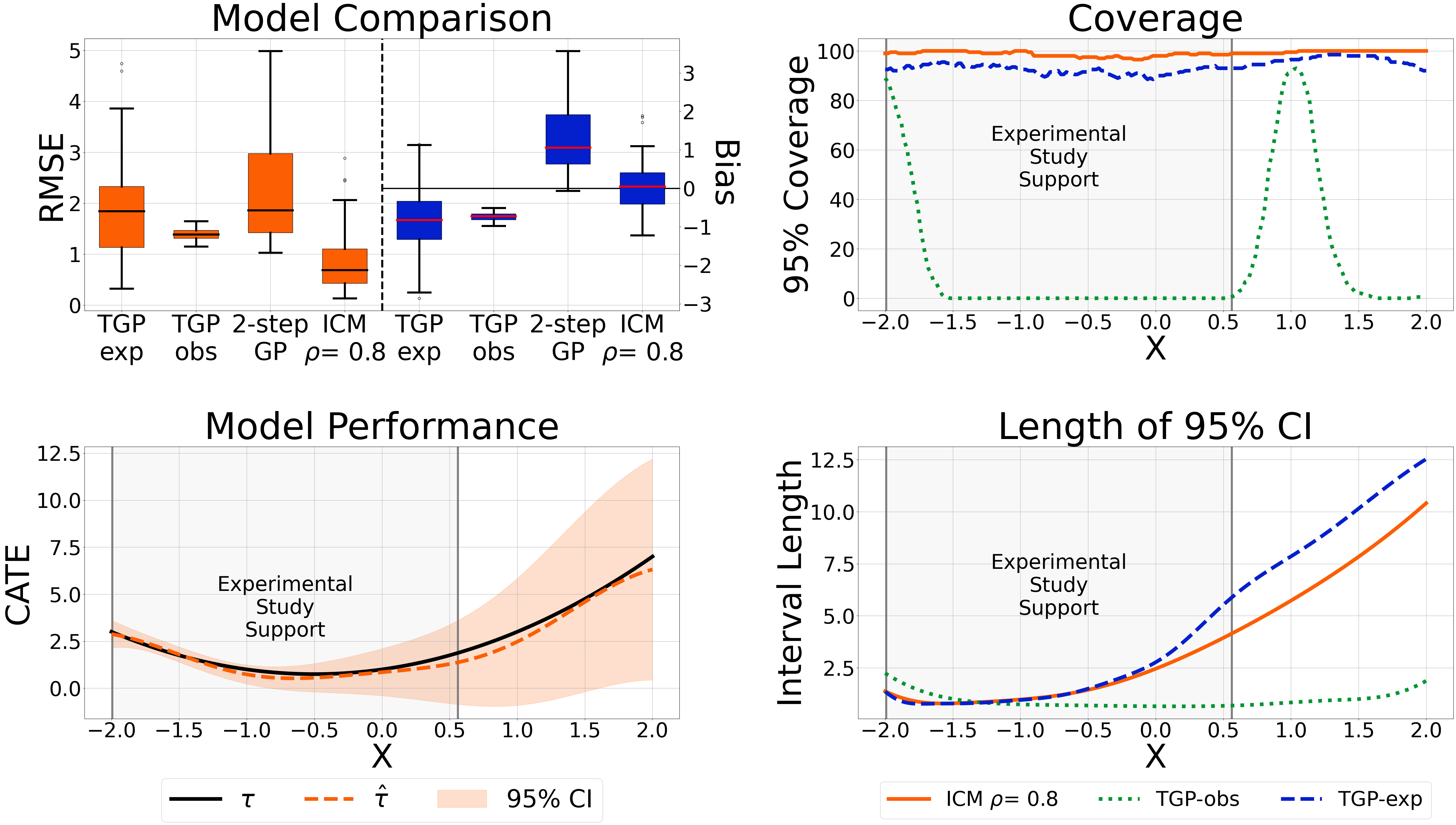
Figure 1: Univariate simulation results. Upper left: Model comparison over 100 simulated datasets Upper right: 95$\%$ Coverage. Lower right: 95$\%$ credible interval length. Lower left: ICM performance in predicting the ground truth. "TGP-exp" and "TGP-obs" are the T-learners with GPs s trained on the RCT and observational data respectively; "2-step GP" is the method of Kallus et al. (2018) with GPs as base learners; Causal-ICM is our proposed method. As Kallus et al. (2018) does not provide a method to compute confidence intervals, the 2-step GP is excluded in the right panels.

The multivariate simulation study was generated similarly with 5 covariates, with some confounding the study participation or the treatment allocation mechanism. More details can be found in Appendix (A.8.2). In the multivariate case (where $\rho=0.3$ was selected), Causal-ICM also produced the lowest average RMSE value ($2.46\pm 0.15$), followed by the T-learner trained on the experimental data ($3.08\pm 0.20$), 2-step method of Kallus et al. (2018) ($3.16\pm 0.16$) and last by the observational-only T-learner ($3.46\pm 0.05$). Here, we report the mean $\pm$ 1 standard error, and results for the bias can be found in Appendix A.8.2. Causal-ICM was again conservative with higher than nominal level coverage (Table 2). The lowest average coverage is again attained by the observational-only T-learner. We note that TGP-exp achieves slightly narrower interval lengths. This is likely due to kernel hyperparameter optimization variability: we expect the Causal-ICM intervals to be narrower when the kernel hyperparameter values are chosen to be the same as TGP-exp.

4.2 Real-World Data Analysis

The Tennessee Student/Teacher Achievement Ratio (STAR) (Achilles et al., 2008) randomised experiment initiated in 1985 studied the impact of class size on student outcomes through standardized test scores from first to third grade. We focus on two ‘treatments’, here corresponding to two experimental conditions: small class size and regular class size. We followed a similar approach to Kallus et al. (2018) and used the real data to produce a ‘confounded’ dataset, corresponding to the observational sample, and a smaller unconfounded dataset, which comprised our RCT data. After removing subjects with missing treatment or outcome values, we were left with a randomised sample of 4218 students. Baseline covariates included gender, race, birth month, birth year, free lunch eligibility and teacher ID. To obtain the ‘experimental’ dataset we sampled randomly only from rural or inner city students. To form the confounded observational dataset, we aggregated all control cases not included in the experimental data. Additionally, for those undergoing treatment, we drew a sample with a down-weighting mechanism applied to individuals whose outcomes fell below the $30^{th}$ percentile. After preprocessing, the unconfounded dataset included 422 students, while the confounded dataset included 2593. Further, 379 students were kept as a validation set.

In order to compare Causal-ICM with existing methods, we require a notion of ground truth. Given the randomised nature of the study, we assume that an unbiased estimate of the CATE can be obtained using a doubly robust estimator, which we then treat as the ground truth. To obtain this, we estimated the propensity score and conditional expectation models using the full dataset, prior to splitting it into the confounded and unconfounded samples (Saito and Yasui, 2020). We note that, in the absence of the true CATE, other performance metrics adapted to the counterfactual nature of the evaluation are also available (Alaa and Van Der Schaar, 2019; Boyer et al., 2023). In the RWD analysis, Causal-ICM achieved the best performance in terms of RMSE followed by the 2-step approach of Kallus et al. (2018) with RF as base learners (Table 2).

Table 1: Multivariate simulation setting:
Average coverage and interval lengths

	Coverage		Length
Nominal	$90\%$	$95\%$	$90\%$	$95\%$
Causal-ICM ($\rho=0.3$)	$98.5\%$	$100\%$	4.72	5.62
TGP-obs	$69\%$	$78\%$	1.01	1.20
TGP-exp	$93\%$	$96.5\%$	4.35	5.18

Table 2: RWD Analysis:
Model comparison

	RMSE
TGP-obs	57.89
TGP-exp	43.17
2-step GP	41.62
2-step RF	39.07
Causal-ICM ($\rho=0.1$)	37.86

TGP-obs and TGP-exp stand for T-learner with GPs as regressors trained on observational or experimental data, respectively. 2-step GP and 2-step RF stand for the 2-step debiasing method proposed by Kallus et al. (2018) with GPs or RF as base learners respectively.

5 Discussion

We have developed Causal-ICM, a rank-2 ICM to combine observational and experimental data to estimate treatment effects for a target population, where the hyperparameter $\rho$ controls the degree of borrowing in an interpretable way. By providing accurate estimates of heterogeneous treatment effects, Causal-ICM has the potential to inform more personalised decision making in medicine. Moreover, by highlighting parts of the population for which treatment effects are highly uncertain, our methodology may guide the design of future trials to improve their representativeness and reduce this uncertainty to a satisfactory level. Although extrapolation is generally challenging, the ICM appears to extrapolate successfully with calibrated uncertainty quantification, achieving reasonable levels of coverage. Nonetheless, it is challenging to guarantee frequentist coverage for Bayesian nonparametric methods, which is one of the limitations of our method. Another limitation is the sensitivity of uncertainty estimates to the kernel hyperparameter optimization, which is an intrinsic challenge of GP s. Future directions or research include the consideration of multiple data sources or multiple treatment arms, imposing a prior distribution on the parameter $\rho$, and incorporating the propensity score into our model. Investigating the partial identification of causal effects under Causal-ICM, especially in regions of extrapolation, is also an important area for future work.

Appendix A Appendix

A.1 Identifiability assumptions

We outline the identifiability assumptions for the CATE in the RCT population below.

1. Consistency of counterfactual outcomes: If $A=a$ then $Y^{a}=Y$.
   The intervention is well defined, there are no hidden versions of the treatment. This assumption can be supported by the study design, i.e. careful implementation of standardized treatment protocols.

2. No interference between individuals of the treatment groups, i.e. one subjects treatment cannot affect another subject’s outcome.

3. No hidden confounding in the trial: $Y^{a}\perp\!\!\!\perp A|\left(\mathbf{x},S=1\right)$
   This assumption is supported by randomization.

4. Positivity of treatment in the trial: for every covariate level $\mathbf{x}$ with positive density in the trial (i.e. $\mathbf{x}\in\mathcal{X}^{\text{e}}$), the probability of being assigned each of the randomized treatments is positive, i.e. $\mathbb{P}\left[A=a|\textbf{x},S=1\right]>0$

A.2 Illustrative example

Figure 2 depicts the differences between single independent GPs and multi-task GPs. Independent GPs excel in regions with observed data but exhibit suboptimal performance during extrapolation. In contrast, Multitask GPs enhance both prediction accuracy and uncertainty quantification in unobserved areas, showcasing superior performance in extrapolation scenarios.

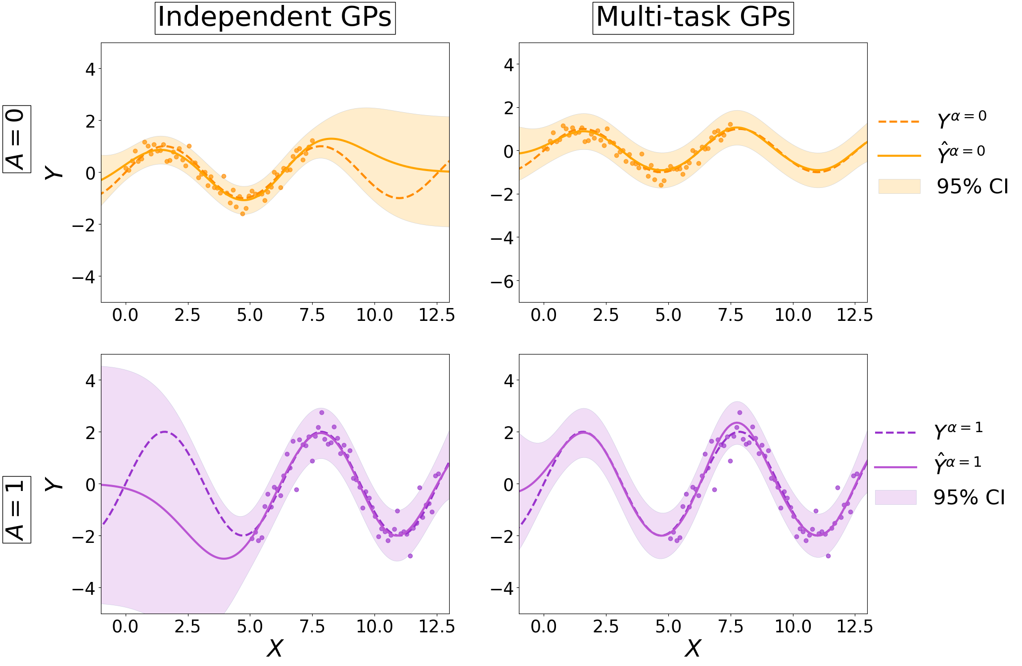
Figure 2: Comparative illustration between Independent GPs and Multitask GP. Here, $A$ represents distinct treatment groups, $Y$ corresponds to the outcome, and $X$ denotes baseline covariates.

A.3 Derivation of Posterior Distribution

The ICM set-up is

$$f^{\text{e}}\left(\mathbf{x}\right) =\alpha_{1}^{\text{e}}u_{1}(\mathbf{x})+\alpha_{2}^{\text{e}}u_{2}(\mathbf{x})$$

$$f^{\text{o}}\left(\mathbf{x}\right) =\alpha_{1}^{\text{o}}u_{1}(\mathbf{x})+\alpha_{2}^{\text{o}}u_{2}(\mathbf{x})$$

where $u_{i}(\mathbf{x})\sim\mathcal{GP}\left(0,k(\mathbf{x},\mathbf{x})\right)$ independently. Suppose we observe $(\mathbf{y}^{\text{e}},X^{\text{e}})$ and $(\mathbf{y}^{\text{o}},X^{\text{o}})$, where the dataset is of size $n_{\text{e}}$ and $n_{\text{o}}$ respectively. The observational model is

$$y^{\text{e}}_{i}=f^{\text{e}}(\mathbf{x}_{i})+\epsilon_{i}^{\text{e}}$$

$$y^{\text{o}}_{i}=f^{\text{o}}(\mathbf{x}_{i})+\epsilon_{i}^{\text{o}}$$

where both $\epsilon^{\text{e}},\epsilon^{\text{o}}$ arise independently from $\mathcal{N}(0,\sigma^{2})$.

We clearly have $\mathbb{E}\left[y_{i}^{\text{e}}\right]=\mathbb{E}\left[y_{i}^{\text{o}}\right]=0$, where the expectation is over both the observation noise and the GP prior. The variance is more interesting. It is not difficult to show that

$$\mathbb{E}\left[y^{\text{e}}_{i}y^{\text{e}}_{j}\right] =\begin{cases}\beta^{\text{e}}k(\mathbf{x}^{\text{e}}_{i},\mathbf{x}^{\text{e}}_{j})+\sigma^{2}\quad&\text{if }i=j\\ \beta^{\text{e}}k(\mathbf{x}^{\text{e}}_{i},\mathbf{x}^{\text{e}}_{j})\quad&\text{otherwise}\end{cases}$$

Similarly, we have

$$\mathbb{E}\left[y^{\text{o}}_{i}y^{\text{o}}_{j}\right] =\begin{cases}\beta^{\text{o}}k(\mathbf{x}^{\text{o}}_{i},\mathbf{x}^{\text{o}}_{j})+\sigma^{2}\quad&\text{if }i=j\\ \beta^{\text{o}}k(\mathbf{x}^{\text{o}}_{i},\mathbf{x}^{\text{o}}_{j})\quad&\text{otherwise}\end{cases}$$

Finally, we have

$$\mathbb{E}\left[y^{\text{e}}_{i}y^{\text{o}}_{j}\right] =\beta^{\text{eo}}k(\mathbf{x}^{\text{e}}_{i},\mathbf{x}^{\text{o}}_{j}).$$

Consider a new test point $\mathbf{x}_{*}$, and we are interested in $f^{\text{e}}(\mathbf{x}_{*})$ and $f^{\text{o}}(\mathbf{x}_{*})$. One can also show that $\mathbb{E}\left[f^{\text{e}}(\mathbf{x}_{*})\right]=\mathbb{E}\left[f^{\text{o}}(\mathbf{x}_{*})\right]=0$, and

$$\mathbb{E}\left[f^{\text{e}}(\mathbf{x}_{*})\,y_{i}^{\text{e}}\right] =\beta^{\text{e}}k(\mathbf{x}^{\text{e}}_{i},\mathbf{x}_{*})$$

$$\mathbb{E}\left[f^{\text{o}}(\mathbf{x}_{*})y_{i}^{\text{o}}\right] =\beta^{\text{o}}k(\mathbf{x}^{\text{o}}_{i},\mathbf{x}_{*})$$

$$\mathbb{E}\left[f^{\text{e}}(\mathbf{x}_{*})y_{i}^{\text{o}}\right] =\beta^{\text{eo}}k(\mathbf{x}^{\text{o}}_{i},\mathbf{x}_{*})$$

$$\mathbb{E}\left[f^{\text{o}}(\mathbf{x}_{*})y_{i}^{\text{e}}\right] =\beta^{\text{eo}}k(\mathbf{x}^{\text{e}}_{i},\mathbf{x}_{*})$$

We now write this in vector form. Let us define

$$\mathbf{y}=\begin{bmatrix}\mathbf{y}^{\text{e}}\\ \mathbf{y}^{\text{o}}\end{bmatrix}$$

which is of length $n_{\text{e}}+n_{\text{o}}$. We can similarly define $X=(X^{\text{e}},X^{\text{o}})$ which is a $(n_{\text{e}}+n_{\text{o}})\times p$ matrix. We then write

$$\mathbf{y}\sim\mathcal{N}\left(\mathbf{0},K(X,X)+\sigma^{2}I\right)$$

where

$$K(X,X)=\begin{bmatrix}\beta^{\text{e}}K(X^{\text{e}},X^{\text{e}})&\beta^{\text{eo}}K(X^{\text{e}},X^{\text{o}})\\ \beta^{\text{eo}}K(X^{\text{o}},X^{\text{e}})&\beta^{\text{o}}K(X^{\text{o}},X^{\text{o}})\end{bmatrix}$$

If we similarly write $\mathbf{f}(\mathbf{x}_{*})=(f^{\text{e}}(\mathbf{x}_{*}),f^{\text{o}}(\mathbf{x}_{*}))$, then we have

$$\begin{bmatrix}\mathbf{y}\\ \mathbf{f}(\mathbf{x}_{*})\end{bmatrix}\sim\mathcal{N}\left(\mathbf{0},\begin{bmatrix}K(X,X)+\sigma^{2}I&K(X,\mathbf{x}_{*})\\ K(\mathbf{x}_{*},X)&K(\mathbf{x}_{*},\mathbf{x}_{*})\end{bmatrix}\right)$$

where

$$K(\mathbf{x}_{*},\mathbf{x}_{*}) =B\otimes k(\mathbf{x}_{*},\mathbf{x}_{*})$$

$$K(X,\mathbf{x}_{*}) =\begin{bmatrix}\beta^{\text{e}}k(\mathbf{x}_{*},X^{\text{e}})&\beta^{\text{eo}}k(\mathbf{x}_{*},X^{\text{e}})\\ \beta^{\text{eo}}k(\mathbf{x}_{*},X^{\text{o}})&\beta^{\text{o}}k(\mathbf{x}_{*},X^{\text{o}}).\end{bmatrix}$$

To clarify, $K(X,\mathbf{x}_{*})$ is a $(n^{\text{o}}+n^{\text{e}})\times 2$ matrix.

One can then use the usual conditional of a Gaussian distribution, which shows that

$$\mathbf{f}(\mathbf{x}_{*})\mid X,\mathbf{y}\sim\mathcal{N}\left(m_{\mathcal{D}}\left(\mathbf{x}_{*}\right),K_{\mathcal{D}}\left(\mathbf{x}_{*},\mathbf{x}_{*}\right)\right)$$

where

$$K_{\mathcal{D}}\left(\mathbf{x}_{*},\mathbf{x}_{*}\right)=K\left(\mathbf{x}_{*},\mathbf{x}_{*}\right)-K(\mathbf{x}_{*},X)\left[K(X,X)+\sigma^{2}I\right]^{-1}K(X,\mathbf{x}_{*}).$$

The posterior mean can similarly be defined as

$$\mathbf{m}_{\mathcal{D}}\left(\mathbf{x}_{*}\right)=K(\mathbf{x}_{*},X)\left[K(X,X)+\sigma^{2}I\right]^{-1}\mathbf{y}.$$

A.4 Proof of Proposition 3.1

Consider first updating the GP with the experimental data points. This gives us

$$\mathbf{f}(\mathbf{x}_{*})\mid X^{\text{e}},\mathbf{y}^{\text{e}}\sim\mathcal{N}\left(m_{\mathcal{D}_{\textnormal{e}}}\left(\mathbf{x}_{*}\right),K_{\mathcal{D}_{\textnormal{e}}}\left(\mathbf{x}_{*},\mathbf{x}_{*}\right)\right)$$

where

$$K_{\mathcal{D}_{\textnormal{e}}}\left(\mathbf{x}_{*},\mathbf{x}_{*}\right) =K\left(\mathbf{x}_{*},\mathbf{x}_{*}\right)-\begin{bmatrix}\beta^{\text{e}}k(\mathbf{x}_{*},X^{\text{e}})&\beta^{\text{eo}}k(\mathbf{x}_{*},X^{\text{e}})\end{bmatrix}^{T}\Sigma_{\text{e}}^{-1}\begin{bmatrix}\beta^{\text{e}}k(\mathbf{x}_{*},X^{\text{e}})&\beta^{\text{eo}}k(\mathbf{x}_{*},X^{\text{e}})\end{bmatrix}$$

where

$$\Sigma_{\text{e}}=\beta^{\text{e}}K(X^{\text{e}},X^{\text{e}})+\sigma^{2}I$$

and $K(\mathbf{x}_{*},\mathbf{x}_{*})=B\otimes k(\mathbf{x}_{*},\mathbf{x}_{*})$. Note that $\begin{bmatrix}\beta^{\text{e}}k(\mathbf{x}_{*},X^{\text{e}})&\beta^{\text{eo}}k(\mathbf{x}_{*},X^{\text{e}})\end{bmatrix}$ is a $n^{\text{e}}\times 2$ matrix. The posterior mean can similarly be defined, but is not our focus here.

We can now simply treat $m_{\mathcal{D}_{\textnormal{e}}}$ and $K_{\mathcal{D}_{\textnormal{e}}}$ as our prior mean and covariance functions respectively, noting that the covariance function can also be written as

$$K_{\mathcal{D}_{\textnormal{e}}}\left(\mathbf{x}_{*},\mathbf{x}_{*}\right)=B\otimes k(\mathbf{x}_{*},\mathbf{x}_{*})-B^{\prime}\otimes k^{\prime}(\mathbf{x}_{*},\mathbf{x}_{*}),$$

where

$$B^{\prime}=\begin{bmatrix}(\beta^{\text{e}})^{2}&\beta^{\text{e}}\beta^{\text{eo}}\\ \beta^{\text{e}}\beta^{\text{eo}}&(\beta^{\text{eo}})^{2}\end{bmatrix},\leavevmode\nobreak\ \leavevmode\nobreak\ \leavevmode\nobreak\ \leavevmode\nobreak\ \leavevmode\nobreak\ \leavevmode\nobreak\ k^{\prime}(\mathbf{x}_{*},\mathbf{x}_{*})=k(\mathbf{x}_{*},X^{\text{e}})^{T}{\Sigma_{\text{e}}}^{-1}k(\mathbf{x}_{*},X^{\text{e}})$$

As in the main paper, let us assume that

$$\begin{bmatrix}\alpha_{1}^{\text{e}}&\alpha_{2}^{\text{e}}\\ \alpha_{1}^{\text{o}}&\alpha_{2}^{\text{o}}\end{bmatrix}=\begin{bmatrix}1&0\\ \rho&\sqrt{1-\rho^{2}}\end{bmatrix},$$

which gives

$$B=\begin{bmatrix}1&\rho\\ \rho&1\end{bmatrix},\quad B^{\prime}=\begin{bmatrix}1&\rho\\ \rho&\rho^{2}\end{bmatrix}.$$

If we now observe $(X^{\text{o}},\mathbf{y}^{\text{o}})$, then we can write the full posterior as

$$\mathbf{f}(\mathbf{x}_{*})\mid X^{\text{e}},\mathbf{y}^{\text{e}},X^{\text{o}},\mathbf{y}^{\text{o}}\sim\mathcal{N}\left(m_{\mathcal{D}}\left(\mathbf{x}_{*}\right),K_{\mathcal{D}}\left(\mathbf{x}_{*},\mathbf{x}_{*}\right)\right).$$

where the key is that

$$K_{\mathcal{D}}\left(\mathbf{x}_{*},\mathbf{x}_{*}\right)=K_{\mathcal{D}_{\textnormal{e}}}\left(\mathbf{x}_{*},\mathbf{x}_{*}\right)-{K}^{\text{o}}_{\mathcal{D}_{\textnormal{e}}}(\mathbf{x}_{*},X^{\text{o}})\left[{K}^{\text{o}}_{\mathcal{D}_{\textnormal{e}}}(X^{\text{o}},X^{\text{o}})+\sigma^{2}I\right]^{-1}{K}^{\text{o}}_{\mathcal{D}_{\textnormal{e}}}(X^{\text{o}},\mathbf{x}_{*})$$

where

$${K}^{\text{o}}_{\mathcal{D}_{\textnormal{e}}}\left(X^{\text{o}},X^{\text{o}}\right) =\beta^{\text{o}}K\left(X^{\text{o}},X^{\text{o}}\right)-(\beta^{\text{eo}})^{2}K^{\prime}\left(X^{\text{o}},X^{\text{o}}\right)$$

$$=K\left(X^{\text{o}},X^{\text{o}}\right)-\rho^{2}K^{\prime}\left(X^{\text{o}},X^{\text{o}}\right)$$

and

$${K}^{\text{o}}_{\mathcal{D}_{\textnormal{e}}}\left(X^{\text{o}},\mathbf{x}^{*}\right) =\begin{bmatrix}\beta^{\text{eo}}k(\mathbf{x}^{*},X^{\text{o}})-\beta^{\text{e}}\beta^{\text{eo}}k^{\prime}(\mathbf{x}^{*},X^{\text{o}}),&\beta^{\text{o}}k(\mathbf{x}^{*},X^{\text{o}})-(\beta^{\text{eo}})^{2}k^{\prime}(\mathbf{x}^{*},X^{\text{o}})\end{bmatrix}$$

$$=\begin{bmatrix}\rho\left(k(\mathbf{x}^{*},X^{\text{o}})-k^{\prime}(\mathbf{x}^{*},X^{\text{o}})\right),&k(\mathbf{x}^{*},X^{\text{o}})-\rho^{2}k^{\prime}(\mathbf{x}^{*},X^{\text{o}})\end{bmatrix}$$

where ${K}^{\text{o}}_{\mathcal{D}_{\textnormal{e}}}\left(X^{\text{o}},\mathbf{x}^{*}\right)$ is a matrix of shape $n^{\text{o}}\times 2$ and ${K}^{\text{o}}_{\mathcal{D}_{\textnormal{e}}}\left(\mathbf{x}^{*},X^{\text{o}}\right)={K}^{\text{o}}_{\mathcal{D}_{\textnormal{e}}}\left(X^{\text{o}},\mathbf{x}^{*}\right)^{T}$.

We thus have the posterior variance of $f^{\textnormal{e}}$ as

$$V^{\text{e}}(\mathbf{x}_{*})= \left(k(\mathbf{x}_{*},\mathbf{x}_{*})-k^{\prime}(\mathbf{x}_{*},\mathbf{x}_{*})\right)$$

$$-\rho^{2}\left(k(\mathbf{x}^{*},X^{\text{o}})-k^{\prime}(\mathbf{x}^{*},X^{\text{o}})\right)^{T}\Sigma^{-1}_{\textnormal{eo}}\left(k(\mathbf{x}^{*},X^{\text{o}})-k^{\prime}(\mathbf{x}^{*},X^{\text{o}})\right)$$

where

$$\Sigma_{\textnormal{eo}} ={K}^{\text{o}}_{\mathcal{D}_{\textnormal{e}}}\left(X^{\text{o}},X^{\text{o}}\right)+\sigma^{2}I$$

$$=K\left(X^{\text{o}},X^{\text{o}}\right)-\rho^{2}K^{\prime}\left(X^{\text{o}},X^{\text{o}}\right)+\sigma^{2}I.$$

The first term is the original posterior covariance given $(X^{\text{e}},\mathbf{y}^{\text{e}})$, whilst the second term is the reduction in variance due to $\mathcal{D}_{\textnormal{o}}=(X^{\text{o}},\mathbf{y}^{\text{o}})$, which we want to control. In other words, we want to upper bound

$$\rho^{2}\left(k(\mathbf{x}^{*},X^{\text{o}})-k^{\prime}(\mathbf{x}^{*},X^{\text{o}})\right)^{T}\Sigma_{\textnormal{eo}}^{-1}\left(k(\mathbf{x}^{*},X^{\text{o}})-k^{\prime}(\mathbf{x}^{*},X^{\text{o}})\right)$$

We now want to write the above term as the posterior variance of a GP. We can guess the following solution and write:

$$V^{\text{e}}(\mathbf{x}_{*})= (1-\rho^{2})\left(k(\mathbf{x}_{*},\mathbf{x}_{*})-k^{\prime}(\mathbf{x}_{*},\mathbf{x}_{*})\right)+\rho^{2}P$$

where

$$P =\left(k(\mathbf{x}_{*},\mathbf{x}_{*})-k^{\prime}(\mathbf{x}_{*},\mathbf{x}_{*})\right)$$

$$-\left(k(\mathbf{x}^{*},X^{\text{o}})-k^{\prime}(\mathbf{x}^{*},X^{\text{o}})\right)^{T}\Sigma_{\textnormal{eo}}^{-1}\left(k(\mathbf{x}^{*},X^{\text{o}})-k^{\prime}(\mathbf{x}^{*},X^{\text{o}})\right).$$

If we can show that $P\geq 0$, then we are done. To see this, note that we can apply Woodbury’s matrix identity which gives

$$\Sigma_{\textnormal{eo}}^{-1} =[\,\,\underbrace{(1-\rho^{2})K^{\prime}\left(X^{\text{o}},X^{\text{o}}\right)}_{A}+\underbrace{K\left(X^{\text{o}},X^{\text{o}}\right)-K^{\prime}\left(X^{\text{o}},X^{\text{o}}\right)+\sigma^{2}I}_{B}\,\,]^{-1}$$

$$=B^{-1}-\underbrace{(B+BA^{-1}B)^{-1}}_{C}$$

which gives

$$P =\left(k(\mathbf{x}_{*},\mathbf{x}_{*})-k^{\prime}(\mathbf{x}_{*},\mathbf{x}_{*})\right)-\left(k(\mathbf{x}^{*},X^{\text{o}})-k^{\prime}(\mathbf{x}^{*},X^{\text{o}})\right)^{T}B^{-1}\left(k(\mathbf{x}^{*},X^{\text{o}})-k^{\prime}(\mathbf{x}^{*},X^{\text{o}})\right)$$

$$+\underbrace{\left(k(\mathbf{x}^{*},X^{\text{o}})-k^{\prime}(\mathbf{x}^{*},X^{\text{o}})\right)^{T}C\left(k(\mathbf{x}^{*},X^{\text{o}})-k^{\prime}(\mathbf{x}^{*},X^{\text{o}})\right)}_{\geq 0}$$

To show the final term is positive, we just need to show that $C$ is positive semi-definite which implies $x^{T}Cx\geq 0$ for any vectors $x$. If $A$ and $B$ are positive definite (PD) and symmetric, then so is $A^{-1}$ and $BA^{-1}B$. The sum of two PD matrices is PD, as is the inverse of a PD matrix, so $C$ is PD. Finally, we see that the remaining first terms in $P$ is simply the regular posterior variance (given $\mathcal{D}_{\textnormal{o}}$) of a GP with kernel $k(\mathbf{x}_{*},\mathbf{x}_{*})-k^{\prime}(\mathbf{x}_{*},\mathbf{x}_{*})$, which is non-negative.

Putting this together then, we have

$$V^{\text{e}}\left(\mathbf{x}_{*}\right)\geq(1-\rho^{2})\,{V}^{\text{e}}_{\mathcal{D}_{\textnormal{e}}}\left(\mathbf{x}_{*}\right)$$

where ${V}^{\text{e}}_{\mathcal{D}_{\textnormal{e}}}$ is the variance conditional on $\mathcal{D}_{\textnormal{e}}=(X^{\text{e}},\mathbf{y}^{\text{e}})$ only.

A.5 Interpreting $\rho$

For further intuition, $\rho$ can be interpreted as a measure of codependence between $f^{\text{e}}$ and $f^{\text{o}}$, as formalised by the following result.

Proposition A.1.

We have $\rho=1$ if and only if

$$\alpha_{1}^{\emph{e}}\alpha_{2}^{\emph{o}}=\alpha_{1}^{\emph{o}}\alpha_{2}^{\emph{e}}$$

Proof.

It is easier to work with $1-\rho^{2}$, where plugging in the values from (1) gives

$$1-\rho^{2}=\frac{\beta^{\text{e}}\beta^{\text{o}}-\left(\beta^{\text{eo}}\right)^{2}}{\beta^{\text{e}}\beta^{\text{o}}}=\frac{\left(\alpha_{1}^{\text{e}}\alpha_{2}^{\text{o}}-\alpha_{1}^{\text{o}}\alpha_{2}^{\text{e}}\right)^{2}}{\beta^{\text{e}}\beta^{\text{o}}}$$

The denominator is positive and finite, so the numerator is thus $0$ if and only if $\alpha_{1}^{\text{e}}\alpha_{2}^{\text{o}}=\alpha_{1}^{\text{o}}\alpha_{2}^{\text{e}}$. ∎

Assuming non-zero coefficients, this is equivalent to the condition $\alpha_{1}^{\text{e}}/\alpha_{1}^{\text{o}}=\alpha_{2}^{\text{e}}/\alpha_{2}^{\text{o}}$, which implies that $f^{\text{e}}$ is a scalar multiple of $f^{\text{o}}$. It is thus intuitive that this results in $\rho=1$, as learning about $f^{\text{o}}$ is equivalent to learning about $f^{\text{e}}$. Finally, another useful observation is that if a single coefficient is 0, we will have $\rho<1$ as long as all other coefficients are non-zero.

A.6 Confounding function

The hidden confounding function $\eta(\mathbf{x})=f^{\text{e}}(\mathbf{x})-f^{\text{o}}(\mathbf{x})$ quantifies the degree to which conditional average treatment effect in the observational study deviates from the conditional average treatment effect in the trial. This may be of independent interest in order to understand the underlying process for treatment assignment or allocation in the real-world outside of the experimental setting. Although our principal focus in the above exposition is on $f^{\text{e}}$, we may also easily obtain a posterior distribution for $\eta(\mathbf{x})$, by considering the joint posterior distribution over $\mathbf{f}(\mathbf{x})$.

A.6.1 Variance of confounding function

Suppose we now want to compute the variance of the confounding function evaluated at $\mathbf{x}_{*}$. This is given by $\eta(\mathbf{x}_{*})=f^{\text{e}}(\mathbf{x}_{*})-f^{o}(\mathbf{x}_{*})$, or in matrix notation $\eta(\mathbf{x}_{*})=\begin{pmatrix}1\\ -1\end{pmatrix}^{T}\mathbf{f}(\mathbf{x}_{*})$. By standard properties of the multivariate Gaussian distribution, it follows that

$$\eta(\mathbf{x}_{*})\mid X,\mathbf{y}\sim\mathcal{N}\left(m^{\text{e}}(\mathbf{x}_{*})-m^{o}(\mathbf{x}_{*}),V_{\eta}(\mathbf{x}_{*})\right),$$

where

$$V_{\eta}(\mathbf{x}_{*}) =\begin{pmatrix}1\\ -1\end{pmatrix}^{T}K_{*}\left(\mathbf{x}_{*},\mathbf{x}_{*}\right)\begin{pmatrix}1\\ -1\end{pmatrix}$$

$$=(\beta^{\text{e}}+\beta^{o}-2\beta^{eo})k(\mathbf{x}_{*},\mathbf{x}_{*})$$

$$-\begin{pmatrix}(\beta^{\text{e}}-\beta^{eo})k(\mathbf{x}_{*},X^{\text{e}})\\ (\beta^{eo}-\beta^{o})k(\mathbf{x}_{*},X^{o})\end{pmatrix}^{T}\left[K(X,X)+\sigma^{2}I\right]^{-1}\begin{pmatrix}(\beta^{\text{e}}-\beta^{eo})k(\mathbf{x}_{*},X^{\text{e}})\\ (\beta^{eo}-\beta^{o})k(\mathbf{x}_{*},X^{o})\\ \end{pmatrix}$$

$$=2(1-\rho)k(\mathbf{x}_{*},X^{\text{e}})-\begin{pmatrix}(1-\rho)k(\mathbf{x}_{*},X^{\text{e}})\\ (\rho-1)k(\mathbf{x}_{*},X^{o})\end{pmatrix}^{T}\left[K(X,X)+\sigma^{2}I\right]^{-1}\begin{pmatrix}(1-\rho)k(\mathbf{x}_{*},X^{\text{e}})\\ (\rho-1)k(\mathbf{x}_{*},X^{o})\\ \end{pmatrix}$$

A.7 Evaluation metrics

The RMSE is defined as:

$$\textnormal{RMSE}=\sqrt{\mathbb{E}\left[\left(\hat{\tau}({X})-\tau(X)\right)^{2}\right]}$$

while the bias is defined as:

$$\textnormal{Bias}=\mathbb{E}\left[\hat{\tau}({X)}-\tau(X)\right].$$

where in both cases $\tau(X)$ is the true value of the CATE, while $\hat{\tau}(X)$ is the estimated value. The expectation is taken over the covariate distribution of the observational study.

A.8 Simulation Settings

A.8.1 Univariate simulation studies

We explore different simulation scenarios based on the complexity of the potential outcomes function, the confounding effect and the CATE. For each simulation setting, we compare our approach with existing ones (T-learner with GPs as regressors on the observational or experimental data, Kallus et al. [2018] 2-step method with GPs as base learners), we compute the coverage of the $90\%$ and $95\%$ credible intervals according to the values of the baseline covariate and the length of those intervals. We contrast those measures of uncertainty with the ones obtained by a T-learner approach using GPs as regressors on the observational or the experimental data. The simulations under consideration are the following:

Simulation 1: Linear Potential Outcomes, linear confounding, linear CATE

Assume that we have continuous baseline covariate $X\sim U\left[-2,2\right]$. The values of $X$ define the trial participation mechanism defined as $S\sim\text{Bernoulli}\left(p_{S}\right)$ where $p_{S}=\frac{\text{exp}\left(-3-3X\right)}{1+\text{exp}\left(-3-3X\right)}$. After selecting all trial participants we assign them randomly to treatment $A\sim\text{Bernoulli}\left(0.5\right)$. The potential outcomes are generated as $Y\left(a\right)=a\tau\left(X\right)+X+\epsilon$, for $a=0,1$, where $\tau\left(X\right)=1+X$ is the CATE and $\epsilon\sim\mathcal{N}\left(0,1\right)$. For the observational study we have $X\sim U\left[-2,2\right]$ and the treatment is generated according to the model $A\sim\text{Bernoulli}\left(e\left(X\right)\right)$ where $\text{logit}\left(e\left(X\right)\right)=-X$. Similarly to the trial the potential outcomes are $Y\left(a\right)=a\tau\left(X\right)+X+U+\epsilon$, for $a=0,1$. $U$ represents the hidden confounding and we generated as $U\sim\mathcal{N}\left(\left(2A-1\right)X,1\right)$.

Simulation 2: Nonlinear Potential Outcomes, linear confounding, nonlinear CATE

Assume that we have continuous baseline covariate $X\sim U\left[-2,2\right]$. The values of $X$ define the trial participation mechanism defined as $S\sim\text{Bernoulli}\left(p_{S}\right)$ where $p_{S}=\frac{\text{exp}\left(-3-3X\right)}{1+\text{exp}\left(-3-3X\right)}$. After selecting all trial participants we assign them randomly to treatment $A\sim\text{Bernoulli}\left(0.5\right)$. The potential outcomes are generated as $Y\left(a\right)=a\tau\left(X\right)+X^{2}-1+\epsilon$, for $a=0,1$, where $\tau\left(X\right)=1+X+X^{2}$ is the CATE and $\epsilon\sim\mathcal{N}\left(0,1\right)$. For the observational study we have $X\sim U\left[-2,2\right]$ and the treatment is generated according to the model $A\sim\text{Bernoulli}\left(e\left(X\right)\right)$ where $\text{logit}\left(e\left(X\right)\right)=-X$. Similarly to the trial the potential outcomes are $Y\left(a\right)=a\tau\left(X\right)+X^{2}-1+U+\epsilon$, for $a=0,1$. $U$ represents the hidden confounding and we generated as $U\sim\mathcal{N}\left(\left(2A-1\right)X,1\right)$.

Simulation 3: Linear Potential Outcomes, linear confounding, linear CATE

Assume that we have continuous baseline covariate $X\sim U\left[-2,2\right]$. The values of $X$ define the trial participation mechanism defined as $S\sim\text{Bernoulli}\left(p_{S}\right)$ where $p_{S}=\frac{\text{exp}\left(-3-3X\right)}{1+\text{exp}\left(-3-3X\right)}$. After selecting all trial participants we assign them randomly to treatment $A\sim\text{Bernoulli}\left(0.5\right)$. The potential outcomes are generated as $Y\left(a\right)=a\tau\left(X\right)+X+\epsilon$, for $a=0,1$, where $\tau\left(X\right)=1+X$ is the CATE and $\epsilon\sim\mathcal{N}\left(0,1\right)$. For the observational study we have $X\sim U\left[-2,2\right]$ and the treatment is generated according to the model $A\sim\text{Bernoulli}\left(e\left(X\right)\right)$ where $\text{logit}\left(e\left(X\right)\right)=-X$. Similarly to the trial the potential outcomes are $Y\left(a\right)=a\tau\left(X\right)+X+U+\epsilon$, for $a=0,1$. $U$ represents the hidden confounding and we generated as $U\sim\mathcal{N}\left(\left(2A-1\right)X,1\right)$.

Simulation 4: Nonlinear Potential Outcomes, linear confounding, nonlinear CATE

Assume that we have continuous baseline covariate $X\sim U\left[-2,2\right]$. The values of $X$ define the trial participation mechanism defined as $S\sim\text{Bernoulli}\left(p_{S}\right)$ where $p_{S}=\frac{\text{exp}\left(-3-3X\right)}{1+\text{exp}\left(-3-3X\right)}$. After selecting all trial participants we assign them randomly to treatment $A\sim\text{Bernoulli}\left(0.5\right)$. The potential outcomes are generated as $Y\left(a\right)=a\tau\left(X\right)+X^{2}-1+\epsilon$, for $a=0,1$, where $\tau\left(X\right)=1+X+X^{2}$ is the CATE and $\epsilon\sim\mathcal{N}\left(0,1\right)$. For the observational study we have $X\sim U\left[-2,2\right]$ and the treatment is generated according to the model $A\sim\text{Bernoulli}\left(e\left(X\right)\right)$ where $\text{logit}\left(e\left(X\right)\right)=-X$. Similarly to the trial the potential outcomes are $Y\left(a\right)=a\tau\left(X\right)+X^{2}-1+U+\epsilon$, for $a=0,1$. $U$ represents the hidden confounding and we generated as $U\sim\mathcal{N}\left(\left(2A-1\right)X,1\right)$.

Simulation 5: Linear Potential Outcomes, nonlinear confounding, linear CATE

Assume that we have continuous baseline covariate $X\sim U\left[-2,2\right]$. The values of $X$ define the trial participation mechanism defined as $S\sim\text{Bernoulli}\left(p_{S}\right)$ where $p_{S}=\frac{\text{exp}\left(-3-3X\right)}{1+\text{exp}\left(-3-3X\right)}$. After selecting all trial participants we assign them randomly to treatment $A\sim\text{Bernoulli}\left(0.5\right)$. The potential outcomes are generated as $Y\left(a\right)=a\tau\left(X\right)+X+\epsilon$, for $a=0,1$, where $\tau\left(X\right)=1+X$ is the CATE and $\epsilon\sim\mathcal{N}\left(0,1\right)$. For the observational study we have $X\sim U\left[-2,2\right]$ and the treatment is generated according to the model $A\sim\text{Bernoulli}\left(e\left(X\right)\right)$ where $\text{logit}\left(e\left(X\right)\right)=-X$. Similarly to the trial the potential outcomes are $Y\left(a\right)=a\tau\left(X\right)+X+U+\epsilon$, for $a=0,1$. $U$ represents the hidden confounding and we generated as $U\sim\mathcal{N}\left(\left(2A-1\right)\text{sin}\left(X-1\right),1\right)$.

Simulation 6: Nonlinear Potential Outcomes, linear confounding, nonlinear CATE

Assume that we have continuous baseline covariate $X\sim U\left[-2,2\right]$. The values of $X$ define the trial participation mechanism defined as $S\sim\text{Bernoulli}\left(p_{S}\right)$ where $p_{S}=\frac{\text{exp}\left(-3-3X\right)}{1+\text{exp}\left(-3-3X\right)}$. After selecting all trial participants we assign them randomly to treatment $A\sim\text{Bernoulli}\left(0.5\right)$. The potential outcomes are generated as $Y\left(a\right)=a\tau\left(X\right)+X^{2}-1+\epsilon$, for $a=0,1$, where $\tau\left(X\right)=1+X+X^{2}$ is the CATE and $\epsilon\sim\mathcal{N}\left(0,1\right)$. For the observational study we have $X\sim U\left[-2,2\right]$ and the treatment is generated according to the model $A\sim\text{Bernoulli}\left(e\left(X\right)\right)$ where $\text{logit}\left(e\left(X\right)\right)=-X$. Similarly to the trial the potential outcomes are $Y\left(a\right)=a\tau\left(X\right)+X^{2}-1+U+\epsilon$, for $a=0,1$. $U$ represents the hidden confounding and we generated as $U\sim\mathcal{N}\left(\left(2A-1\right)\text{sin}\left(X-1\right),1\right)$.

Simulation 7: Linear Potential Outcomes, linear confounding, linear CATE

Assume that we have continuous baseline covariate $X\sim U\left[-2,2\right]$. The values of $X$ define the trial participation mechanism defined as $S\sim\text{Bernoulli}\left(p_{S}\right)$ where $p_{S}=\frac{\text{exp}\left(-3-3X\right)}{1+\text{exp}\left(-3-3X\right)}$. After selecting all trial participants we assign them randomly to treatment $A\sim\text{Bernoulli}\left(0.5\right)$. The potential outcomes are generated as $Y\left(a\right)=a\tau\left(X\right)+X+\epsilon$, for $a=0,1$, where $\tau\left(X\right)=1+X$ is the CATE and $\epsilon\sim\mathcal{N}\left(0,1\right)$. For the observational study we have $X\sim U\left[-2,2\right]$ and the treatment is generated according to the model $A\sim\text{Bernoulli}\left(e\left(X\right)\right)$ where $\text{logit}\left(e\left(X\right)\right)=-X$. Similarly to the trial the potential outcomes are $Y\left(a\right)=a\tau\left(X\right)+X+U+\epsilon$, for $a=0,1$. $U$ represents the hidden confounding and we generated as $U\sim\mathcal{N}\left(\left(2A-1\right)\text{sin}\left(X-1\right),1\right)$.

Simulation 8: Linear Potential Outcomes, linear confounding, nonlinear CATE

Assume that we have continuous baseline covariate $X\sim U\left[-2,2\right]$. The values of $X$ define the trial participation mechanism defined as $S\sim\text{Bernoulli}\left(p_{S}\right)$ where $p_{S}=\frac{\text{exp}\left(-3-3X\right)}{1+\text{exp}\left(-3-3X\right)}$. After selecting all trial participants we assign them randomly to treatment $A\sim\text{Bernoulli}\left(0.5\right)$. The potential outcomes are generated as $Y\left(a\right)=a\tau\left(X\right)+X^{2}-1+\epsilon$, for $a=0,1$, where $\tau\left(X\right)=1+X+X^{2}$ is the CATE and $\epsilon\sim\mathcal{N}\left(0,1\right)$. For the observational study we have $X\sim U\left[-2,2\right]$ and the treatment is generated according to the model $A\sim\text{Bernoulli}\left(e\left(X\right)\right)$ where $\text{logit}\left(e\left(X\right)\right)=-X$. Similarly to the trial the potential outcomes are $Y\left(a\right)=a\tau\left(X\right)+X^{2}-1+U+\epsilon$, for $a=0,1$. $U$ represents the hidden confounding and we generated as $U\sim\mathcal{N}\left(\left(2A-1\right)\text{sin}\left(X-1\right),1\right)$.

Results: Univariate Case

According to Figure 3, the ICM approach performs equally good or outperforms all other methods. The cases where our approach shows similar performance with Kallus et al. [2018] method is when the confounding function is linear, which is expected as Kallus et al. [2018] modelling framework assumes linear functional form of confounding. In terms of coverage, both of $95\%$ and of $90\%$, we see in Figures 6 and 7 that ICM demonstrates higher coverage rates than the other two methods, indicating a more conservative approach to uncertainty. The T-learner trained on observational data shows the worst coverage rates, while in most cases the T-learner trained on experimental data achieves near optimat average coverage rate. Nevertheless, ICM is the only method demonstrating high coverage rates (even if it’s conservative) across the covariate support of the observational study, whily the T-lerner trained on observational data, in some cases (simulation 6) deteriorates outside the support of the experimental study. In terms of credible interval length, according to Figure 8 and Figure 9, the narrowest intervals are provided by the T-learner trained on observational data. In most simulation cases, the ICM offers the widest intervals, except for Simulation 1, where the T-learner trained on experimental data offers the widest. Figures 10, 11 and 12 the model fits of the two T-learner models and the Causal-ICM are demonstrated. Although there are cases where Causal-ICM has low precision in point predictions outside the support of the RCT we notice that we have appropriate variance inflation covering the true CATE function.

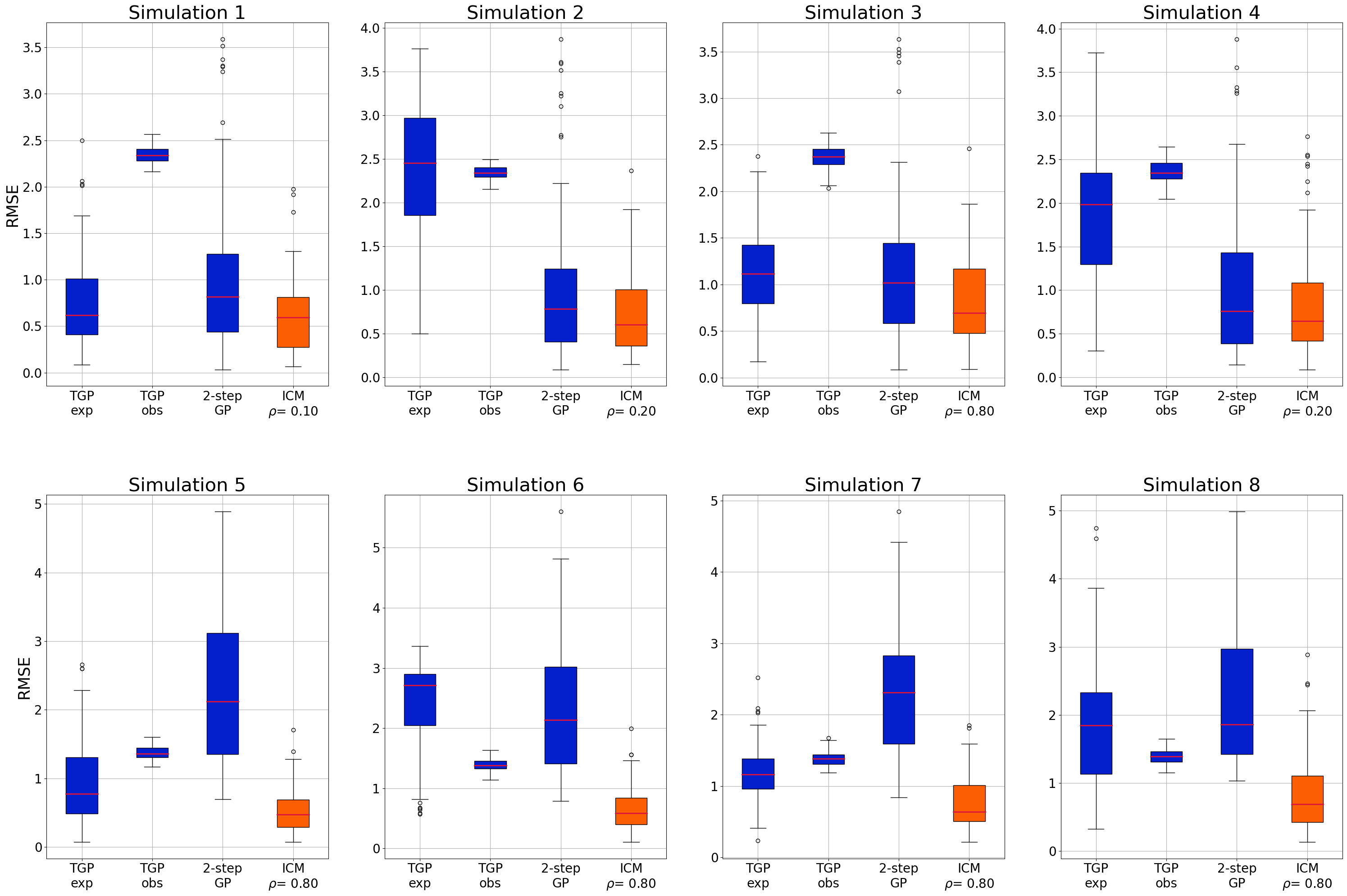
Figure 3: Model comparison for the univariate simulations using the distribution of RMSE obtained through 100 simulated datasets. "GP T-learner exp" and "GP T-learner obs" and stand for the T-learner approach using GPs as regressors trained on the experimental and observational data respectively and "Kallus GP" stands for Kallus et al. [2018] 2-step method with GPs as base learners.

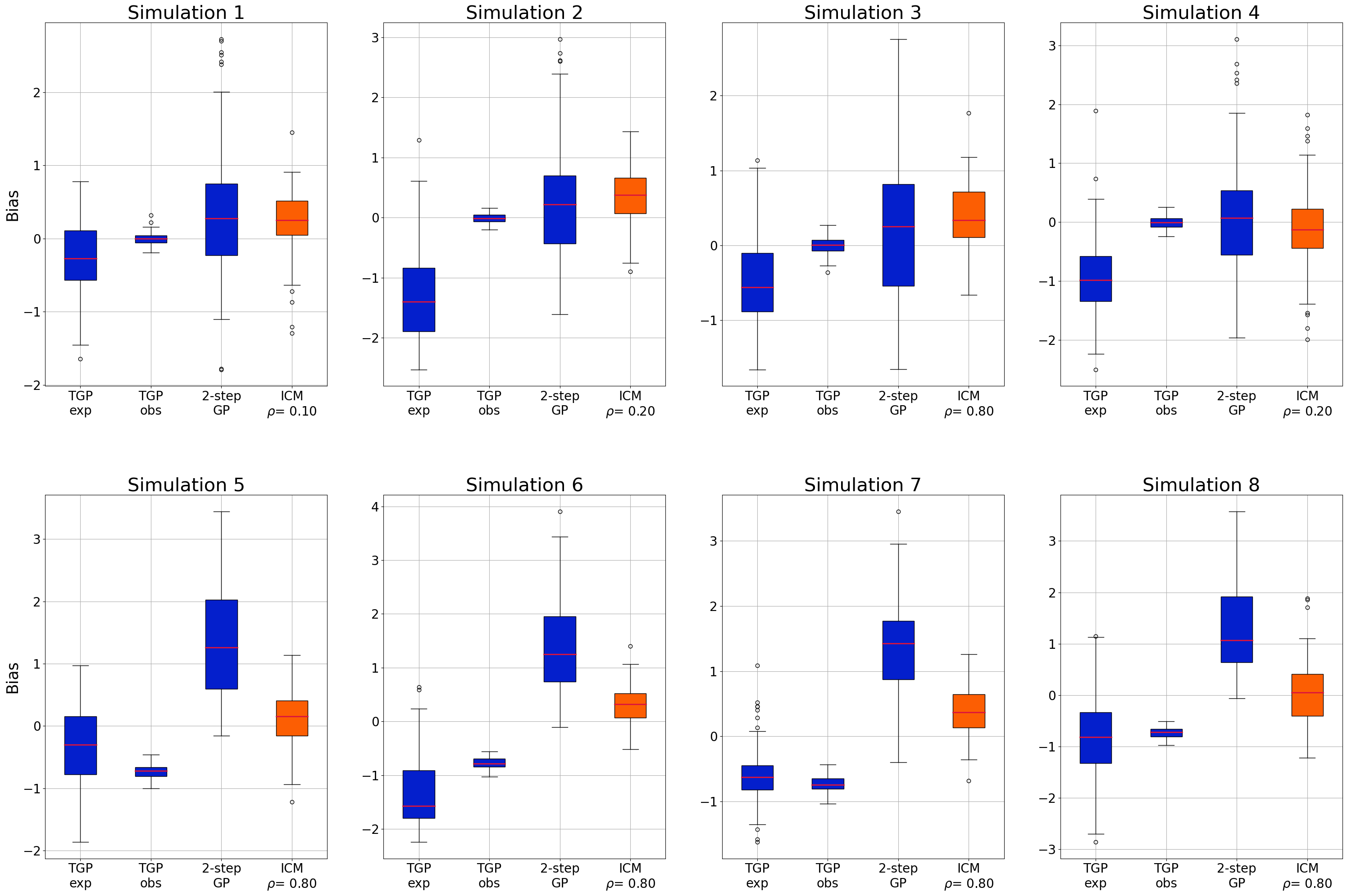
Figure 4: Model comparison for the univariate simulations using the distribution of the Bias obtained through 100 simulated datasets. "GP T-learner exp" and "GP T-learner obs" and stand for the T-learner approach using GPs as regressors trained on the experimental and observational data respectively and "Kallus GP" stands for Kallus et al. [2018] 2-step method with GPs as base learners.

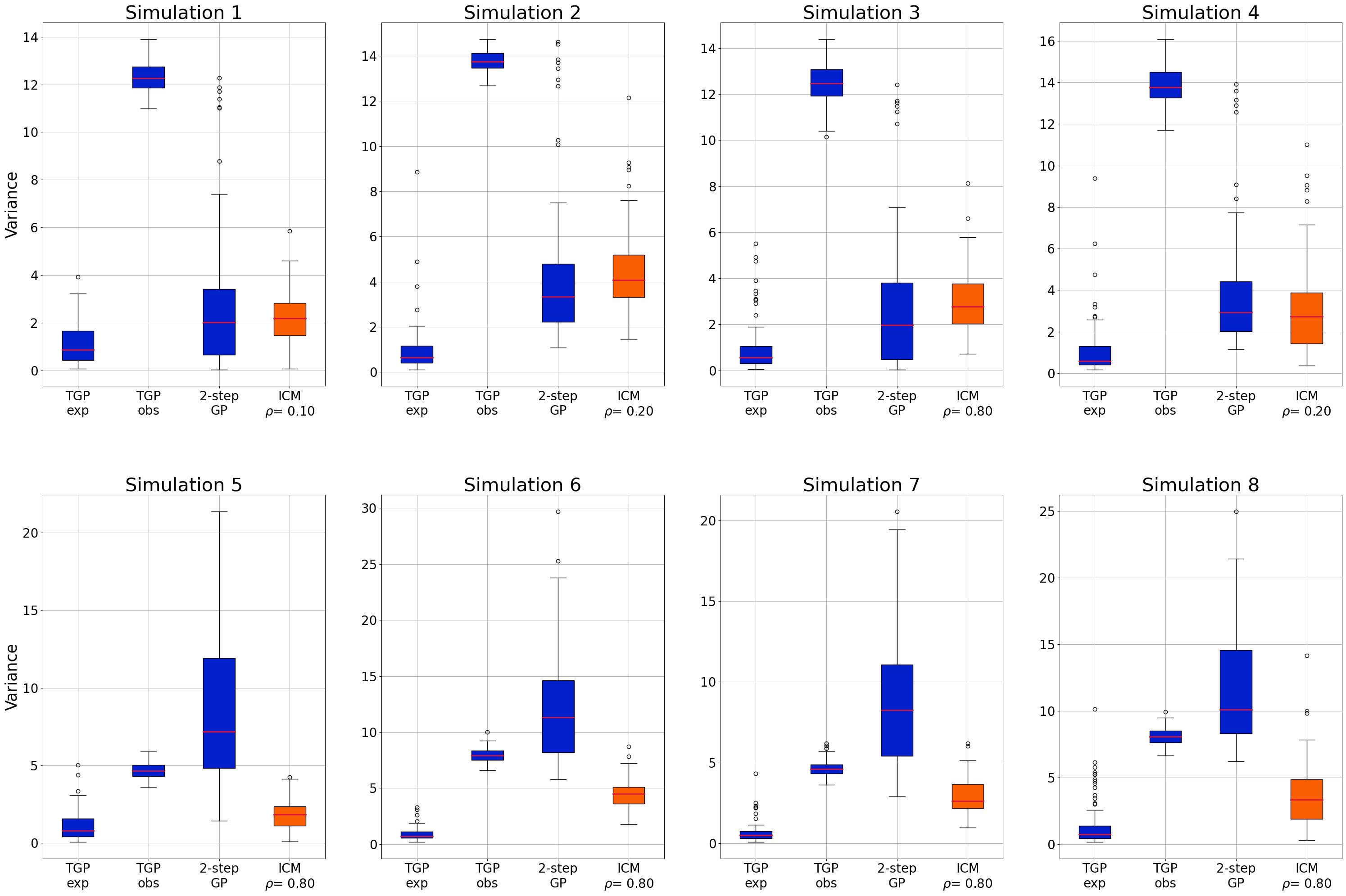
Figure 5: Model comparison for the univariate simulations using the distribution of the Variance obtained through 100 simulated datasets. "GP T-learner exp" and "GP T-learner obs" and stand for the T-learner approach using GPs as regressors trained on the experimental and observational data respectively and "Kallus GP" stands for Kallus et al. [2018] 2-step method with GPs as base learners.

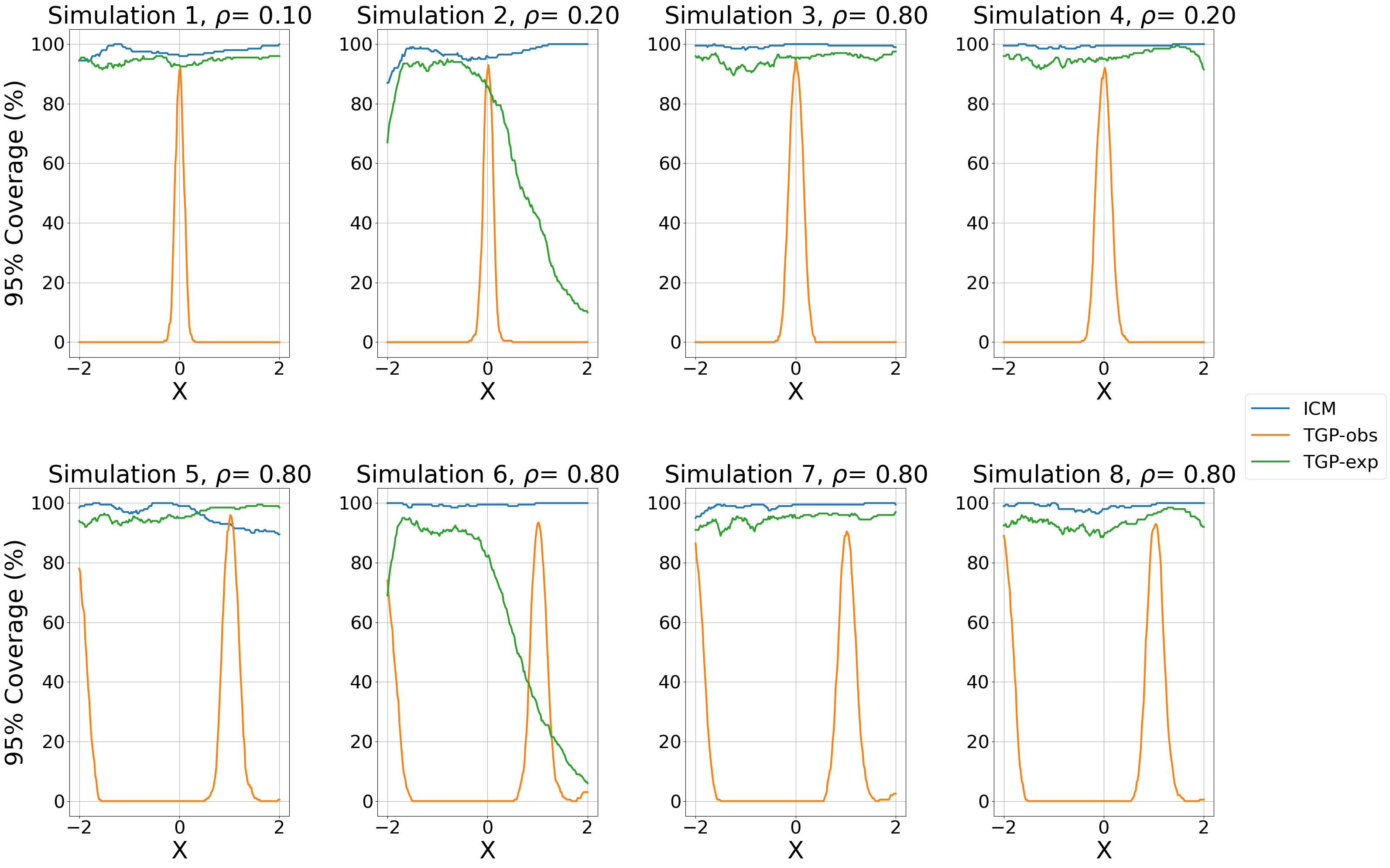
Figure 6: Coverage of $95\%$ credible interval in univariate simulation settings. ICM is contrasted with T-learner approaches with GPs as regressors trained on experimental or observational data separately

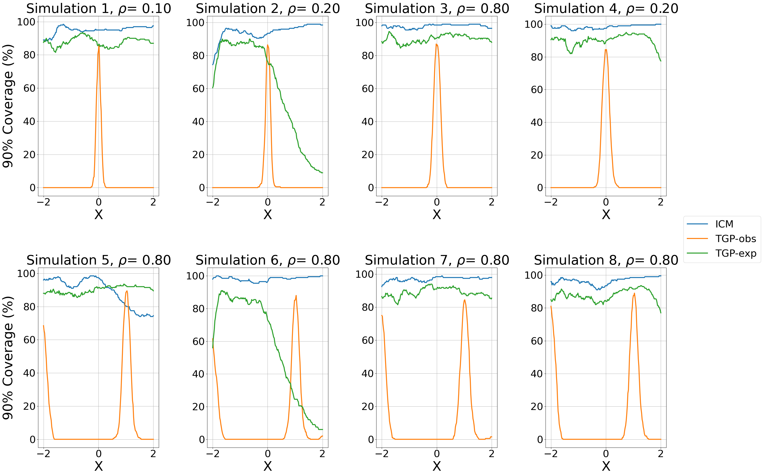
Figure 7: Coverage of $90\%$ credible interval in univariate simulation settings. ICM is contrasted with T-learner approaches with GPs as regressors trained on experimental or observational data separately

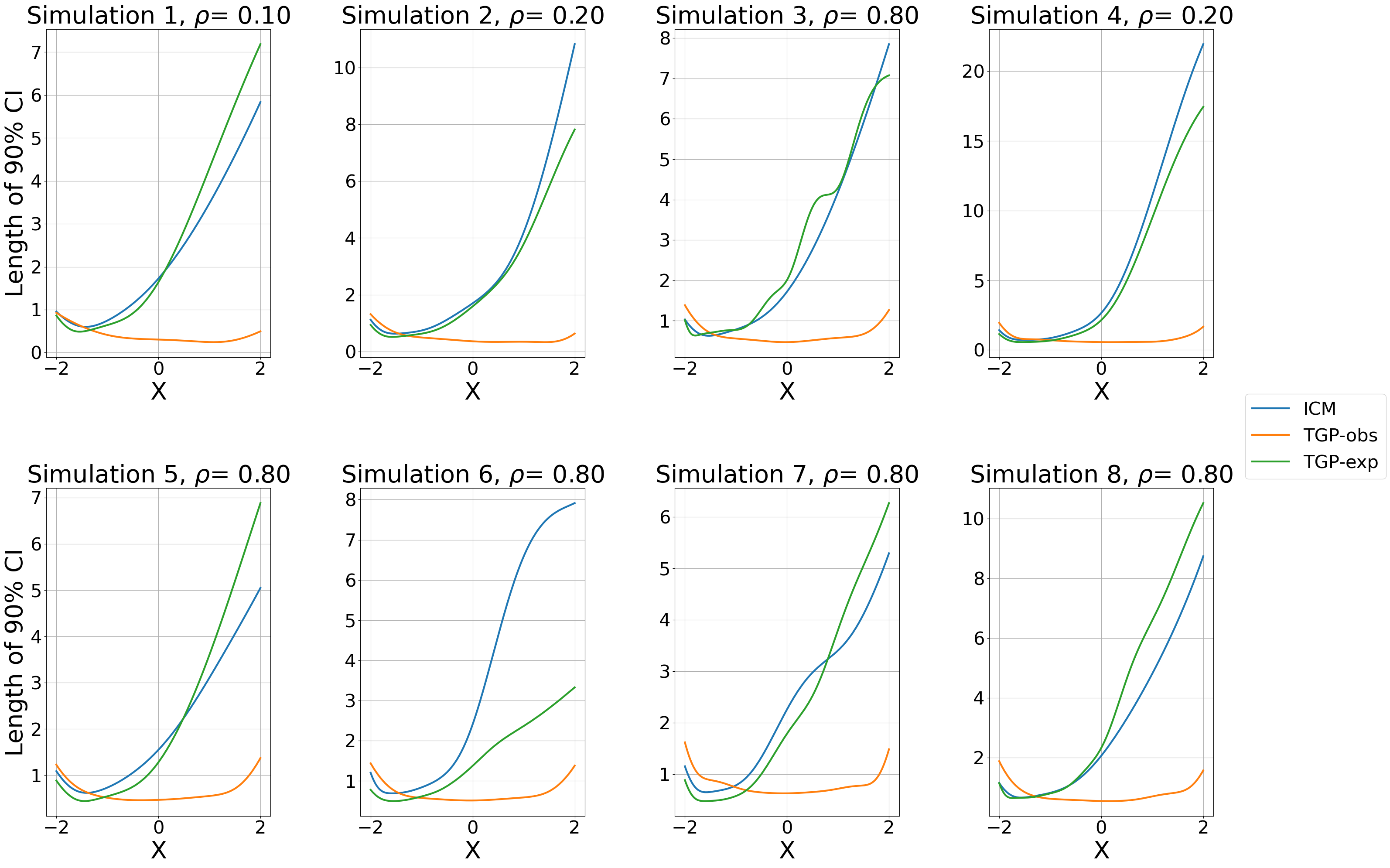
Figure 8: Length of $90\%$ credible interval in univariate simulation settings. ICM is contrasted with T-learner approaches with GPs as regressors trained on experimental or observational data separately

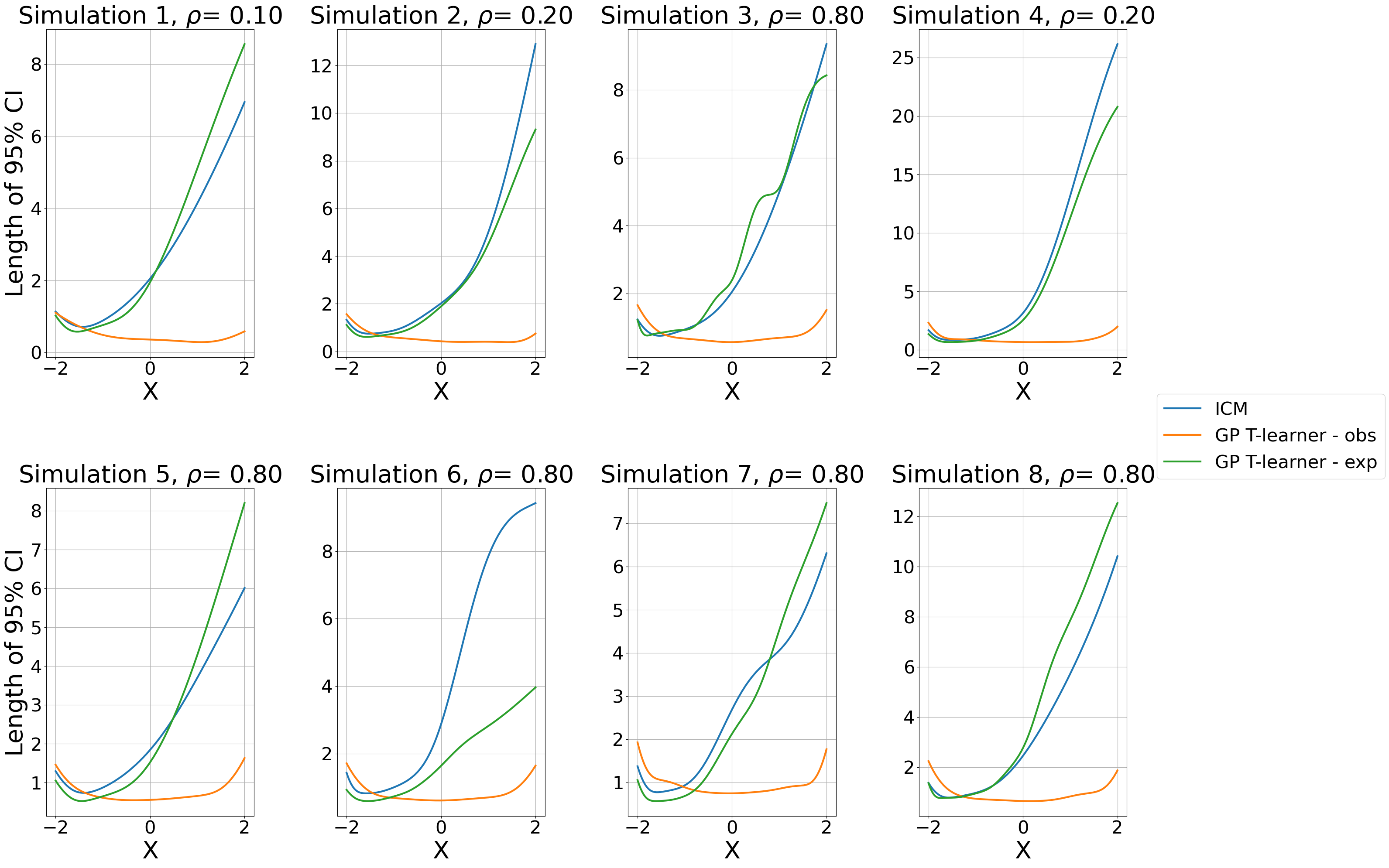
Figure 9: Length of $95\%$ credible interval in univariate simulation settings. ICM is contrasted with T-learner approaches with GPs as regressors trained on experimental or observational data separately

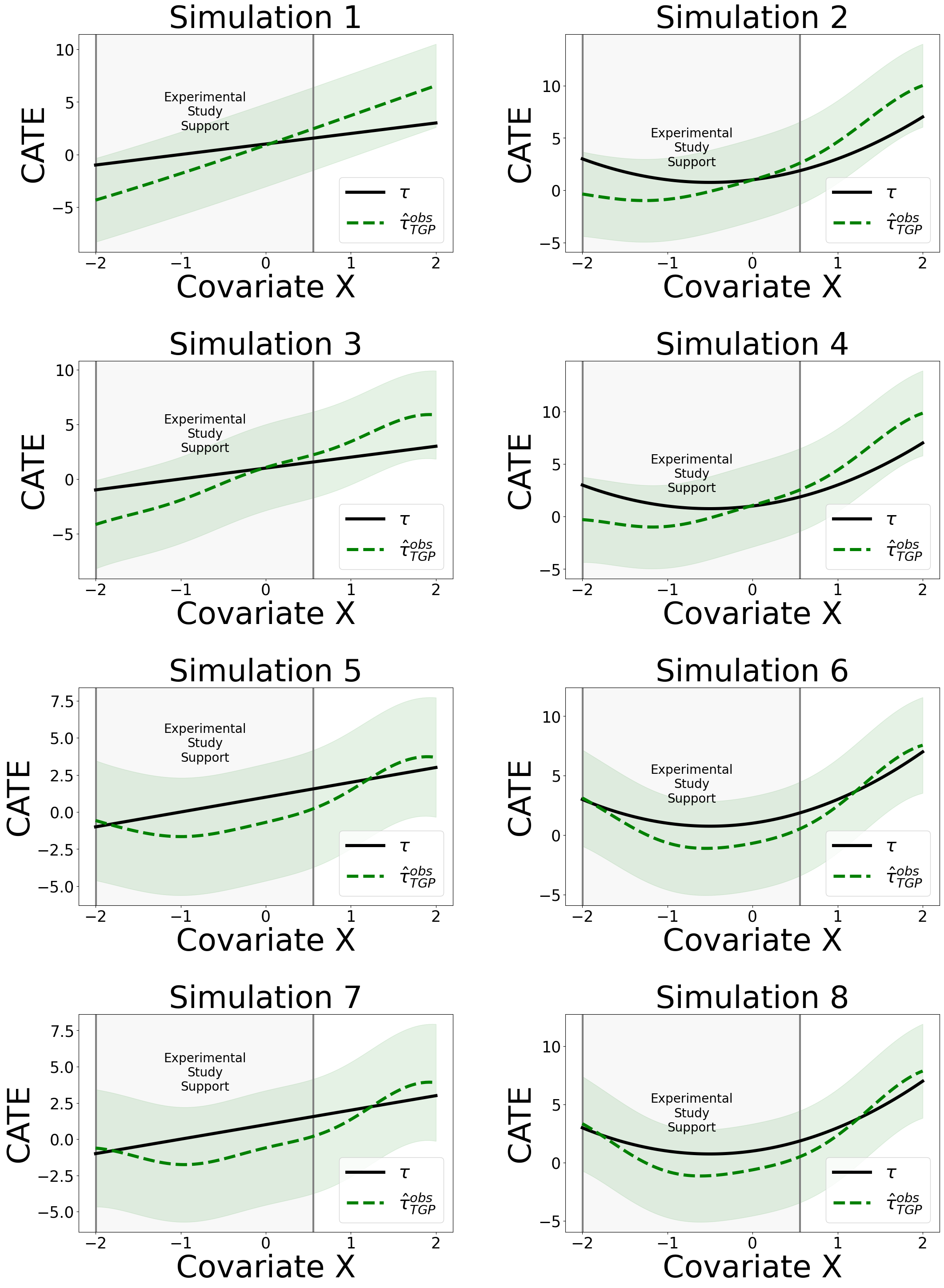
Figure 10: Model fit for the T-learner trained on the observational data alone.

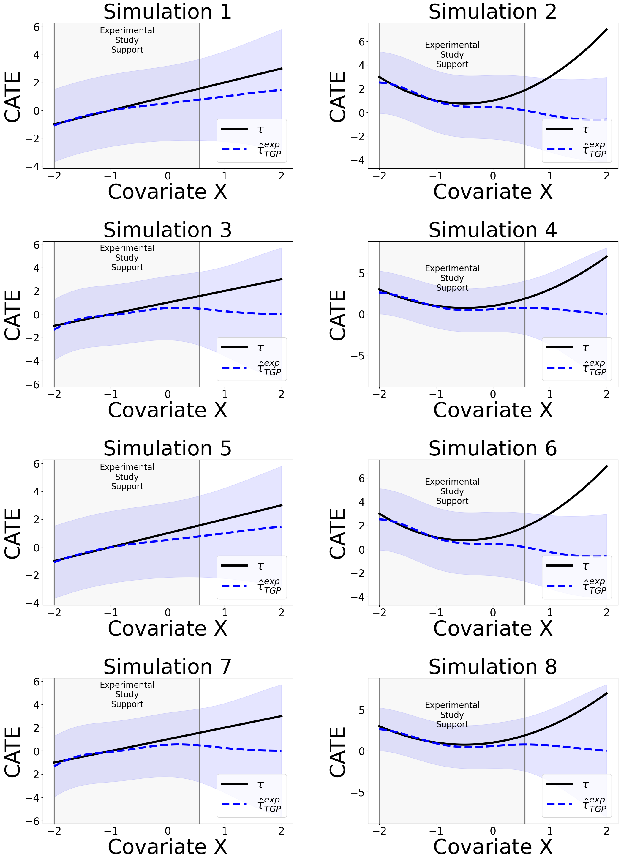
Figure 11: Model fit for the T-learner trained on the experimental data alone.

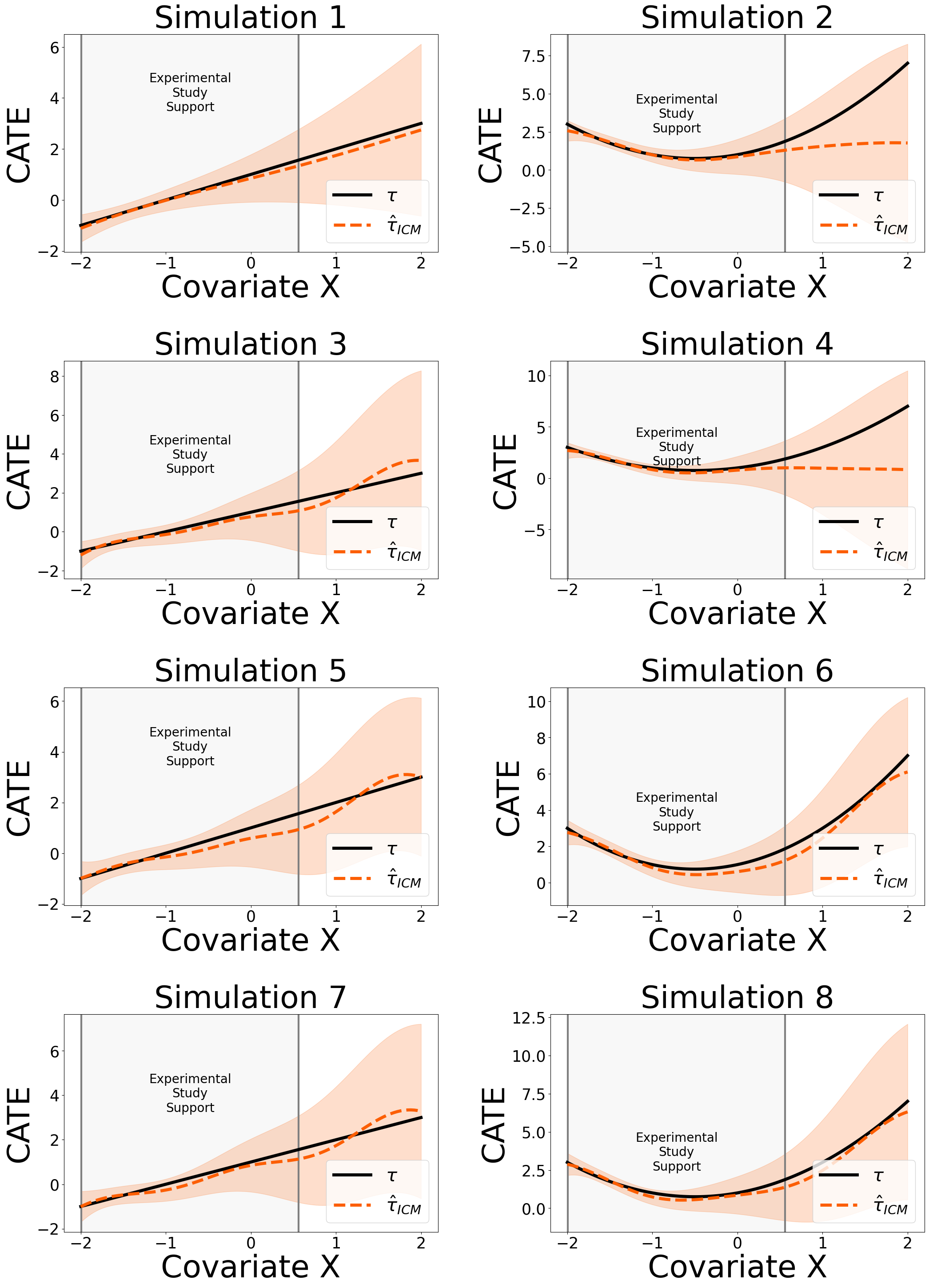
Figure 12: Model fit for the Causal-ICM

A.8.2 Multivariate simulation studies

Similar to the univariate case, in the multivariate case we vary the complexity of the confounding and the CATE function, but we choose to explore only cases with nonlinear potential outcomes functions.

Simulation 1: Noninear Potential Outcomes, linear confounding, linear CATE

Assume that we have five continuous baseline covariate $X_{j}\sim U\left[-2,2\right]$, where $j=1,\cdots,5$. The values of $X$ define the trial participation mechanism defined as $S\sim\text{Bernoulli}\left(p_{S}\right)$ where $p_{S}=\frac{\text{exp}\left(-10-8X_{1}-8X_{2}\right)}{1+\text{exp}\left(-10-8X_{1}-8X_{2}\right)}$. After selecting all trial participants we assign them randomly to treatment $A\sim\text{Bernoulli}\left(0.5\right)$. The potential outcomes are generated as $Y\left(a\right)=a\tau\left(X\right)+\sum_{j=1}^{5}X_{j}+\epsilon$, for $a=0,1$, where $\tau\left(X\right)=1+X_{1}+X_{2}$ is the CATE and $\epsilon\sim\mathcal{N}\left(0,1\right)$. For the observational study we have $X_{j}\sim U\left[-2,2\right]$, where $j=1,\cdots,5$, and the treatment is generated according to the model $A\sim\text{Bernoulli}\left(e\left(X\right)\right)$ where $\text{logit}\left(e\left(X\right)\right)=-\left(X_{1}+X_{2}\right)$. Similarly to the trial the potential outcomes are $Y\left(a\right)=a\tau\left(X\right)+\sum_{j=1}^{5}X_{j}+U+\epsilon$, for $a=0,1$. $U$ represents the hidden confounding and we generated as $U\sim\mathcal{N}\left(\left(2A-1\right)\left(X_{1}+X_{2}\right),1\right)$.

Simulation 2: Noninear Potential Outcomes, linear confounding, nonlinear CATE

Assume that we have five continuous baseline covariate $X_{j}\sim U\left[-2,2\right]$, where $j=1,\cdots,5$. The values of $X$ define the trial participation mechanism defined as $S\sim\text{Bernoulli}\left(p_{S}\right)$ where $p_{S}=\frac{\text{exp}\left(-10-8X_{1}-8X_{2}\right)}{1+\text{exp}\left(-10-8X_{1}-8X_{2}\right)}$. After selecting all trial participants we assign them randomly to treatment $A\sim\text{Bernoulli}\left(0.5\right)$. The potential outcomes are generated as $Y\left(a\right)=a\tau\left(X\right)+\sum_{j=1}^{5}X_{j}+\epsilon$, for $a=0,1$, where $\tau\left(X\right)=1+X_{1}+X_{1}^{2}+X_{2}+X_{2}^{2}$ is the CATE and $\epsilon\sim\mathcal{N}\left(0,1\right)$. For the observational study we have $X_{j}\sim U\left[-2,2\right]$, where $j=1,\cdots,5$, and the treatment is generated according to the model $A\sim\text{Bernoulli}\left(e\left(X\right)\right)$ where $\text{logit}\left(e\left(X\right)\right)=-\left(X_{1}+X_{2}\right)$. Similarly to the trial the potential outcomes are $Y\left(a\right)=a\tau\left(X\right)+\sum_{j=1}^{5}X_{j}+U+\epsilon$, for $a=0,1$. $U$ represents the hidden confounding and we generated as $U\sim\mathcal{N}\left(\left(2A-1\right)\left(X_{1}+X_{2}\right),1\right)$.

Simulation 3: Noninear Potential Outcomes, nonlinear confounding, linear CATE

Assume that we have five continuous baseline covariate $X_{j}\sim U\left[-2,2\right]$, where $j=1,\cdots,5$. The values of $X$ define the trial participation mechanism defined as $S\sim\text{Bernoulli}\left(p_{S}\right)$ where $p_{S}=\frac{\text{exp}\left(-10-8X_{1}-8X_{2}\right)}{1+\text{exp}\left(-10-8X_{1}-8X_{2}\right)}$. After selecting all trial participants we assign them randomly to treatment $A\sim\text{Bernoulli}\left(0.5\right)$. The potential outcomes are generated as $Y\left(a\right)=a\tau\left(X\right)+\sum_{j=1}^{5}X_{j}+\epsilon$, for $a=0,1$, where $\tau\left(X\right)=1+X_{1}+X_{2}$ is the CATE and $\epsilon\sim\mathcal{N}\left(0,1\right)$. For the observational study we have $X_{j}\sim U\left[-2,2\right]$, where $j=1,\cdots,5$, and the treatment is generated according to the model $A\sim\text{Bernoulli}\left(e\left(X\right)\right)$ where $\text{logit}\left(e\left(X\right)\right)=-\left(X_{1}+X_{2}\right)$. Similarly to the trial the potential outcomes are $Y\left(a\right)=a\tau\left(X\right)+\sum_{j=1}^{5}X_{j}+U+\epsilon$, for $a=0,1$. $U$ represents the hidden confounding and we generated as $U\sim\mathcal{N}\left(\left(2A-1\right)\left(\text{sin}\left(X_{1}\right)+\text{sin}\left(X_{2}\right)\right),1\right)$.

Simulation 4: Noninear Potential Outcomes, nonlinear confounding, nonlinear CATE

Assume that we have five continuous baseline covariate $X_{j}\sim U\left[-2,2\right]$, where $j=1,\cdots,5$. The values of $X$ define the trial participation mechanism defined as $S\sim\text{Bernoulli}\left(p_{S}\right)$ where $p_{S}=\frac{\text{exp}\left(-10-8X_{1}-8X_{2}\right)}{1+\text{exp}\left(-10-8X_{1}-8X_{2}\right)}$. After selecting all trial participants we assign them randomly to treatment $A\sim\text{Bernoulli}\left(0.5\right)$. The potential outcomes are generated as $Y\left(a\right)=a\tau\left(X\right)+\sum_{j=1}^{5}X_{j}+\epsilon$, for $a=0,1$, where $\tau\left(X\right)=1+X_{1}+X_{1}^{2}+X_{2}+X_{2}^{2}$ is the CATE and $\epsilon\sim\mathcal{N}\left(0,1\right)$. For the observational study we have $X_{j}\sim U\left[-2,2\right]$, where $j=1,\cdots,5$, and the treatment is generated according to the model $A\sim\text{Bernoulli}\left(e\left(X\right)\right)$ where $\text{logit}\left(e\left(X\right)\right)=-\left(X_{1}+X_{2}\right)$. Similarly to the trial the potential outcomes are $Y\left(a\right)=a\tau\left(X\right)+\sum_{j=1}^{5}X_{j}+U+\epsilon$, for $a=0,1$. $U$ represents the hidden confounding and we generated as $U\sim\mathcal{N}\left(\left(2A-1\right)\left(\text{sin}\left(X_{1}\right)+\text{sin}\left(X_{2}\right)\right),1\right)$.

Results: Multivariate Case

According to Figure 13, the ICM approach outperforms all other methods. According to Table 3, ICM shows higher than optimal average coverage rates, both for $90\%$ and $95\%$ coverage, indicating a conservative view towards uncertainty. Near optimal average coverage rate is indicated by the T-leraner approach trained on experimental data, while the worst average coverage is indicated by the T-learner on the observational data. In terms of average credible interval length, according to 4, the narrowest intervals are provided by the T-learner trained on observational data. In most simulation cases, the ICM offers the widest intervals, except for Simulation 1, where the T-learner trained on experimental data offers the widest.

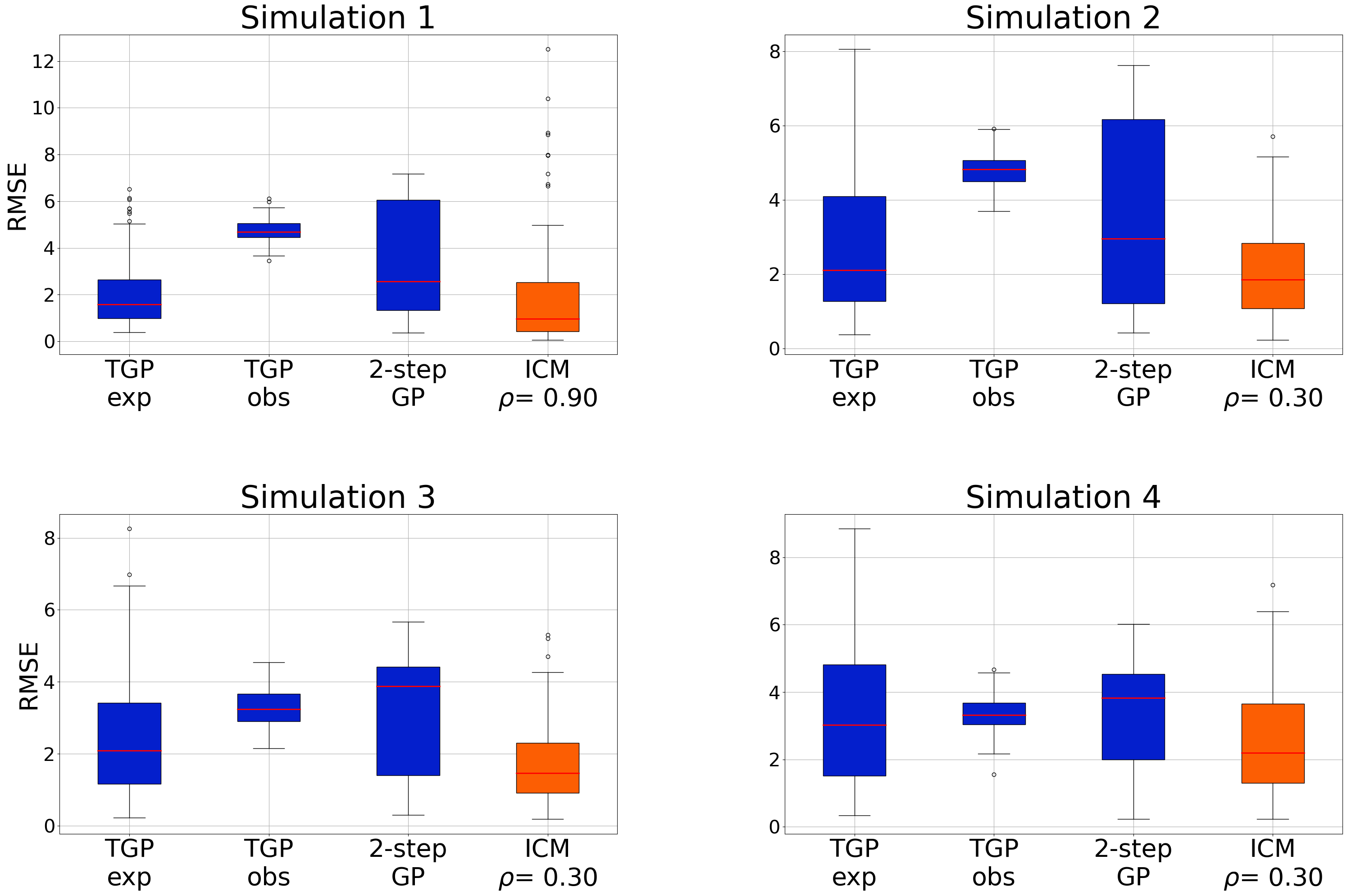
Figure 13: Multivariate simulation results. Boxplots of the RMSEs for each model, trained on 100 different datasets

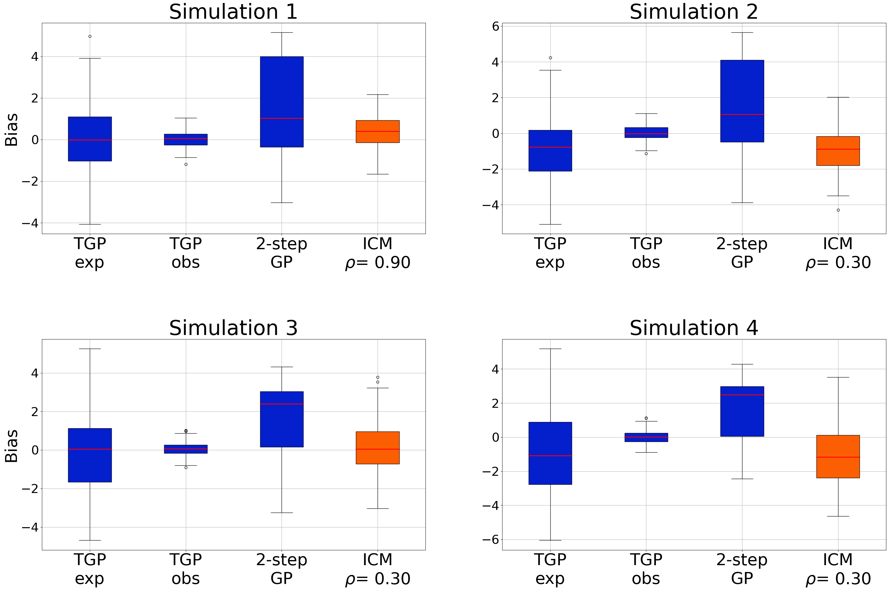
Figure 14: Multivariate simulation results. Boxplots of the Bias for each model, trained on 100 different datasets

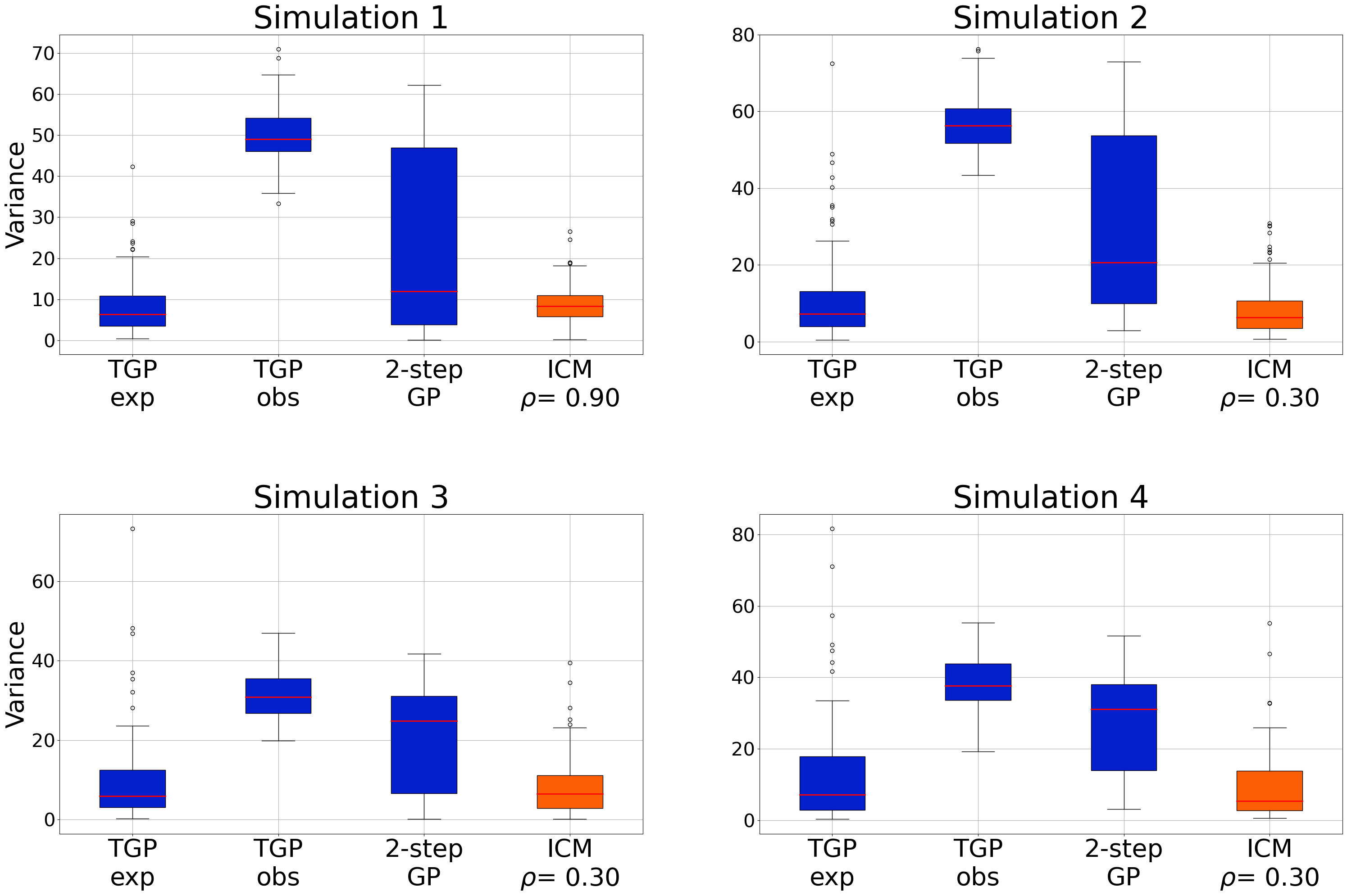
Figure 15: Multivariate simulation results. Boxplots of the Variance for each model, trained on 100 different datasets

Table 3: Average $90\%$ and $95\%$ Coverage rate for multivariate simulation settings

		$90\%$ Coverage	$95\%$ Coverage
Sim. 1	ICM ($\rho=0.9$)	$99.5\%$	$100.0\%$
	GP T-learner (observational)	$2.5\%$	$5.5\%$
	GP T-learner (experimental)	$95.0\%$	$99.5\%$
Sim. 2	ICM ($\rho=0.3$)	$98.5\%$	$100.0\%$
	GP T-learner (observational)	$60.5\%$	$77.0\%$
	GP T-learner (experimental)	$92.5\%$	$96.5\%$
Sim. 3	ICM ($\rho=0.3$)	$99.5\%$	$100.0\%$
	GP T-learner (observational)	$3.0\%$	$5.5\%$
	GP T-learner (experimental)	$97.5\%$	$99.0\%$
Sim. 4	ICM ($\rho=0.3$)	$98.5\%$	$100.0\%$
	GP T-learner (observational)	$69.0\%$	$78.0\%$
	GP T-learner (experimental)	$93.0\%$	$96.5\%$

Table 4: Average length of $90\%$ and $95\%$ credible interval for multivariate simulation settings

		$90\%$ CI	$95\%$ CI
Sim. 1	ICM ($\rho=0.9$)	6.05	7.20
	GP T-learner (observational)	1.34	1.60
	GP T-learner (experimental)	9.03	10.76
Sim. 2	ICM ($\rho=0.3$)	8.01	9.55
	GP T-learner (observational)	2.31	2.75
	GP T-learner (experimental)	7.64	9.10
Sim. 3	ICM ($\rho=0.3$)	10.36	12.34
	GP T-learner (observational)	1.38	1.64
	GP T-learner (experimental)	10.14	12.08
Sim. 4	ICM ($\rho=0.3$)	4.72	5.63
	GP T-learner (observational)	1.01	1.20
	GP T-learner (experimental)	4.35	5.18

References

- Achilles et al. (2008) C. Achilles, H. P. Bain, F. Bellott, J. Boyd-Zaharias, J. Finn, J. Folger, J. Johnston, and E. Word. Tennessee’s Student Teacher Achievement Ratio (STAR) project, Apr. 2008. URL http://arxiv.org/abs/1106.6251.
- Alaa and Van Der Schaar (2019) A. Alaa and M. Van Der Schaar. Validating causal inference models via influence functions. In K. Chaudhuri and R. Salakhutdinov, editors, Proceedings of the 36th International Conference on Machine Learning, volume 97 of Proceedings of Machine Learning Research, pages 191–201. PMLR, 09–15 Jun 2019. URL https://proceedings.mlr.press/v97/alaa19a.html.
- Alaa and van der Schaar (2017) A. M. Alaa and M. van der Schaar. Bayesian Inference of Individualized Treatment Effects using Multi-task Gaussian Processes. In Advances in Neural Information Processing Systems, volume 30. Curran Associates, Inc., 2017. URL https://proceedings.neurips.cc/paper/2017/hash/6a508a60aa3bf9510ea6acb021c94b48-Abstract.html.
- Alvarez et al. (2012) M. A. Alvarez, L. Rosasco, and N. D. Lawrence. Kernels for Vector-Valued Functions: a Review, Apr. 2012. URL http://arxiv.org/abs/1106.6251. arXiv:1106.6251 [cs, math, stat].
- Boyer et al. (2023) C. B. Boyer, I. J. Dahabreh, and J. A. Steingrimsson. Assessing model performance for counterfactual predictions, 2023.
- Brantner et al. (2023) C. L. Brantner, T.-H. Chang, T. Q. Nguyen, H. Hong, L. Di Stefano, and E. A. Stuart. Methods for Integrating Trials and Non-Experimental Data to Examine Treatment Effect Heterogeneity, Mar. 2023. URL http://arxiv.org/abs/2302.13428. arXiv:2302.13428 [stat].
- Caron et al. (2022) A. Caron, I. Manolopoulou, and G. Baio. Counterfactual Learning with Multioutput Deep Kernels. Transactions on Machine Learning Research, 2022. ISSN 2835-8856. URL https://openreview.net/forum?id=iGREAJdULX.
- Colnet et al. (2023) B. Colnet, I. Mayer, G. Chen, A. Dieng, R. Li, G. Varoquaux, J.-P. Vert, J. Josse, and S. Yang. Causal inference methods for combining randomized trials and observational studies: a review, Jan. 2023. URL http://arxiv.org/abs/2011.08047. arXiv:2011.08047 [stat].
- Dahabreh and Hernán (2019) I. J. Dahabreh and M. A. Hernán. Extending inferences from a randomized trial to a target population. European Journal of Epidemiology, 34(8):719–722, Aug. 2019. ISSN 1573-7284. doi: 10.1007/s10654-019-00533-2.
- Degtiar and Rose (2023) I. Degtiar and S. Rose. A review of generalizability and transportability. Annual Review of Statistics and Its Application, 10(1):501–524, 2023. doi: 10.1146/annurev-statistics-042522-103837. URL https://doi.org/10.1146/annurev-statistics-042522-103837.
- Frieden (2017) T. R. Frieden. Evidence for health decision making — beyond randomized, controlled trials. New England Journal of Medicine, 377(5):465–475, 2017. doi: 10.1056/NEJMra1614394. URL https://www.nejm.org/doi/full/10.1056/NEJMra1614394.
- GPy (2012) GPy. GPy: A Gaussian process framework in Python. http://github.com/SheffieldML/GPy, 2012.
- Hahn et al. (2020) P. R. Hahn, J. S. Murray, and C. M. Carvalho. Bayesian Regression Tree Models for Causal Inference: Regularization, Confounding, and Heterogeneous Effects (with Discussion). Bayesian Analysis, 15(3):965–1056, Sept. 2020. ISSN 1936-0975, 1931-6690. doi: 10.1214/19-BA1195. Publisher: International Society for Bayesian Analysis.
- Huang et al. (2023) B. Huang, C. Chen, J. Liu, and S. Sivaganisan. Gpmatch: A bayesian causal inference approach using gaussian process covariance function as a matching tool. Frontiers in Applied Mathematics and Statistics, 9, 2023. ISSN 2297-4687. doi: 10.3389/fams.2023.1122114. URL https://www.frontiersin.org/articles/10.3389/fams.2023.1122114.
- Kallus et al. (2018) N. Kallus, A. M. Puli, and U. Shalit. Removing Hidden Confounding by Experimental Grounding. In Advances in Neural Information Processing Systems, volume 31. Curran Associates, Inc., 2018. URL https://papers.nips.cc/paper/2018/hash/566f0ea4f6c2e947f36795c8f58ba901-Abstract.html.
- Künzel et al. (2019) S. R. Künzel, J. S. Sekhon, P. J. Bickel, and B. Yu. Metalearners for estimating heterogeneous treatment effects using machine learning. Proceedings of the National Academy of Sciences, 116(10):4156–4165, Feb. 2019. ISSN 1091-6490. doi: 10.1073/pnas.1804597116. URL http://dx.doi.org/10.1073/pnas.1804597116.
- Lin and Evans (2023) X. Lin and R. J. Evans. Many Data: Combine Experimental and Observational Data through a Power Likelihood, Apr. 2023. URL http://arxiv.org/abs/2304.02339. arXiv:2304.02339 [math, stat].
- National Academies of Sciences, Engineering, and Medicine (2022) National Academies of Sciences, Engineering, and Medicine. Improving Representation in Clinical Trials and Research: Building Research Equity for Women and Underrepresented Groups. The National Academies Press, Washington, DC, 2022. ISBN 978-0-309-27820-1. doi: 10.17226/26479. URL https://nap.nationalacademies.org/catalog/26479/improving-representation-in-clinical-trials-and-research-building-research-equity.
- Saito and Yasui (2020) Y. Saito and S. Yasui. Counterfactual cross-validation: Stable model selection procedure for causal inference models, 2020.
- Vargas-Guzman and Warrick (1999) J. Vargas-Guzman and A. Warrick. Geostatistics for natural resources evaluation. Journal of Environmental Quality, 28(3):1044–1044, 1999. doi: https://doi.org/10.2134/jeq1999.00472425002800030046x. URL https://acsess.onlinelibrary.wiley.com/doi/abs/10.2134/jeq1999.00472425002800030046x.
- Wager and Athey (2018) S. Wager and S. Athey. Estimation and Inference of Heterogeneous Treatment Effects using Random Forests. Journal of the American Statistical Association, 113(523):1228–1242, July 2018. ISSN 0162-1459. doi: 10.1080/01621459.2017.1319839. URL https://doi.org/10.1080/01621459.2017.1319839. Publisher: Taylor & Francis _eprint: https://doi.org/10.1080/01621459.2017.1319839.
- Witty et al. (2020) S. Witty, K. Takatsu, D. Jensen, and V. Mansinghka. Causal inference using gaussian processes with structured latent confounders. In Proceedings of the 37th International Conference on Machine Learning, ICML’20. JMLR.org, 2020.
- Wu and Yang (2022) L. Wu and S. Yang. Integrative -learner of heterogeneous treatment effects combining experimental and observational studies. In Proceedings of the First Conference on Causal Learning and Reasoning, pages 904–926. PMLR, June 2022. URL https://proceedings.mlr.press/v177/wu22a.html. ISSN: 2640-3498.
- Yang et al. (2022) S. Yang, D. Zeng, and X. Wang. Improved Inference for Heterogeneous Treatment Effects Using Real-World Data Subject to Hidden Confounding, Jan. 2022. URL http://arxiv.org/abs/2007.12922. arXiv:2007.12922 [stat].