Improving Generalization and Convergence by Enhancing Implicit Regularization

Abstract

In this work, we propose an Implicit Regularization Enhancement (IRE) framework to accelerate the discovery of flat solutions in deep learning, thereby improving generalization and convergence. Specifically, IRE decouples the dynamics of flat and sharp directions, which boosts the sharpness reduction along flat directions while maintaining the training stability in sharp directions. We show that IRE can be practically incorporated with generic base optimizers without introducing significant computational overload. Experiments show that IRE consistently improves the generalization performance for image classification tasks across a variety of benchmark datasets (CIFAR-10/100, ImageNet) and models (ResNets and ViTs). Surprisingly, IRE also achieves a $2\times$ speed-up compared to AdamW in the pre-training of Llama models (of sizes ranging from 60M to 229M) on datasets including Wikitext-103, Minipile, and Openwebtext. Moreover, we provide theoretical guarantees, showing that IRE can substantially accelerate the convergence towards flat minima in Sharpness-aware Minimization (SAM).

1 Introduction

Deep learning has achieved remarkable success across a variety of fields, including computer vision, scientific computing, and artificial intelligence. The core challenge in deep learning lies in how to train deep neural networks (DNNs) efficiently to achieve superior performance. Understanding and improving the generalization and convergence of commonly-used optimizers, such stochastic gradient descent (SGD) (Robbins and Monro, 1951; Rumelhart et al., 1986), in deep learning is crucial for both theoretical research and practical applications.

Notably, optimizers often exhibit a preference for certain solutions in training DNNs. For instance, SGD and its variants consistently converge to solutions that generalize well, even when DNNs are highly over-parameterized and there are many solutions that generalize poorly. This phenomenon is referred to as implicit regularization in the literature (Neyshabur et al., 2014; Zhang et al., 2017).

The most popular explanation for implicit regularization is that SGD and its variants tend to converge to flat minima (Keskar et al., 2016; Wu et al., 2017), and flat minima generalize better (Hochreiter and Schmidhuber, 1997; Jiang et al., 2019). However, the process of this implicit sharpness regularization occurs at a very slow pace, as demonstrated in works such as Blanc et al. (2020), Li et al. (2022), and Ma et al. (2022). Consequently, practitioners often use a large learning rate (LR) and extend the training time even when the loss no longer decreases, ensuring the convergence to flatter minima (He et al., 2016; Goyal et al., 2017; Hoffer et al., 2017). Nevertheless, the largest allowable LR is constrained by the need to maintain training stability. In addition, Foret et al. (2021) proposed SAM, which aims to explicitly regularize sharpness during training and has achieved superior performance across a variety of tasks.

Our contributions can be summarized as follows:

• We propose an Implicit Regularization Enhancement (IRE) framework to speed up the convergence towards flatter minima. As suggested by works like Blanc et al. (2020), Li et al. (2022) and Ma et al. (2022), the implicit sharpness reduction often occurs at a very slow pace, along flat directions. Inspired by this picture, IRE particularly accelerates the dynamics along flat directions, while keeping sharp directions’ dynamics unchanged. As such, IRE can boost the implicit sharpness reduction substantially without hurting training stability. For a detailed illustration of this mechanism, we refer to Section 2.

• We then provide a practical IRE framework, which can be efficiently incorporated with generic base optimizers. We evaluate the performance of this practical IRE in both vision and language tasks. For vision tasks, IRE consistently improves the generalization performance of popular optimizers like SGD, Adam, and SAM in classifying the CIFAR-10/100 and ImageNet datasets with ResNets (He et al., 2016) and vision transformers (ViTs) (Dosovitskiy et al., 2020). For language modelling, we consider the pre-training of Llama models (Touvron et al., 2023) of various sizes, finding that IRE surprisingly can accelerate the pre-training convergence. Specifically, we observe a remarkable $2.0\times$ speedup compared to AdamW in the scenarios we examined, despite IRE being primarily motivated to speed up the convergence to flat solutions.

• Lastly, we provide theoretical guarantees showing that IRE can achieves a $\Theta(1/\rho)$-time acceleration over the base SAM algorithm in minimizing the trace of Hessian, where $\rho\in(0,1)$ is a small hyperparameter in SAM.

1.1 Related works

Implicit regularization. There have been extensive attempts to explain the mystery of implicit regularization in deep learning (see the survey by Vardi (2023) and references therein). Here, we focus on works related to implicit sharpness regularization. Wu et al. (2018; 2022) and Ma and Ying (2021) provided an explanation of implicit sharpness regularization from a dynamical stability perspective. Moreover, in-depth analysis of SGD dynamics near global minima shows that the SGD noise (Blanc et al., 2020; Li et al., 2022; Ma et al., 2022; Damian et al., 2021) and the edge of stability (EoS)-driven (Wu et al., 2018; Cohen et al., 2021) oscillations (Even et al., 2024) can drive SGD/GD towards flatter minima. Additional studies explored how training components, including learning rate and batch size (Jastrzębski et al., 2017), normalization (Lyu et al., 2022), cyclic LR (Wang and Wu, 2023), influence this sharpness regularization. Furthermore, some works have provided theoretical evidence explaining the superior generalization of flat minima for neural networks (Ma and Ying, 2021; Mulayoff et al., 2021; Wu and Su, 2023; Gatmiry et al., 2023; Wen et al., 2023b). Our work is inspired by this line of research, aiming to boost implicit sharpness regularization by decoupling the dynamics along flat and sharp directions.

Sharpness-aware minimization. IRE shares the same motivation as SAM in enhancing sharpness regularization, although their specific approaches differ significantly. It is worth noting that the per-step computational cost of SAM is twice that of base optimizers. Consequently, there have been numerous attempts to reduce the computational cost of SAM (Kwon et al., 2021; Liu et al., 2022; Du et al., 2021; Mi et al., 2022; Mueller et al., 2024). In contrast, the per-step computational cost of IRE is only approximately 1.1 times that of base optimizers (see Table 5). Moreover, we provide both theoretical and experimental evidence demonstrating that the mechanism of IRE in boosting sharpness regularization is nearly orthogonal to that of SAM.

Optimizers for large language model (LLM) pre-training. (Momentum) SGD (Sutskever et al., 2013; Nesterov, 1983) and its adaptive variants like Adagrad (Duchi et al., 2011), RMSProp (Tieleman, 2012), and Adam (Kingma and Ba, 2014) have been widely used in DNN training. Despite the efforts in designing better adaptive gradient methods (Liu et al., 2019a; Luo et al., 2019; Heo et al., 2020; Zhuang et al., 2020; Xie et al., 2022b; a), AdamW(Adam+decoupled weight decay) (Loshchilov and Hutter, 2017) has become the default optimizer in LLM pre-training. Recently, Chen et al. (2024) discovered Lion by searching the space of adaptive first-order optimizers; Liu et al. (2024) introduced Sophia, a scalable second-order optimizer. In this paper, we instead empirically demonstrate that IRE can accelerate the convergence of AdamW in the pre-training of Llama models.

1.2 Notations

Throughout this paper, let $\mathcal{L}:\mathbb{R}^{p}\mapsto\mathbb{R}_{\geqslant 0}$ be the function of total loss, where $p$ denotes the number of model parameters. For a $\mathcal{C}^{2}$-submanifold $\mathcal{M}$ in $\mathbb{R}^{p}$, we denote the tangent space of $\mathcal{M}$ at $\bm{\theta}\in\mathcal{M}$ as $\mathcal{T}_{\bm{\theta}}\mathcal{M}$, which is a linear subspace in $\mathbb{R}^{p}$. For $f\in\mathcal{C}^{1}(\mathcal{M})$ and $\bm{\theta}\in\mathcal{M}$, let $\nabla_{\mathcal{M}}f(\bm{\theta}):=\mathbb{\mathcal{Q}}_{\mathcal{T}_{\bm{\theta}}\mathcal{M}}\nabla f(\bm{\theta})$ denote the Riemannian gradient, where $\mathcal{Q}_{\mathcal{T}_{\bm{\theta}}\mathcal{M}}:\mathbb{R}^{p}\mapsto\mathbb{R}^{p}$ denotes the orthogonal projection to $\mathcal{T}_{\bm{\theta}}\mathcal{M}$. For a symmetric matrix $A\in\mathbb{R}^{p\times p}$, its eigen pairs are denoted as $\{(\lambda_{i},\bm{u}_{i})\}_{i\in[p]}$ with the order $\lambda_{1}\geqslant\cdots\geqslant\lambda_{p}$. We use $P_{i:j}(A)=\sum_{k=i}^{j}\bm{u}_{k}\bm{u}_{k}^{\top}$ to denote the projection operator onto $\mathrm{span}\{\bm{u}_{i},\dots,\bm{u}_{j}\}$. Denote $\mathcal{N}(\bm{\mu},\Sigma)$ as the Gaussian distribution with mean $\bm{\mu}$ and covariance matrix $\Sigma$, and $\mathbb{U}(\mathcal{S})$ as the uniform distribution over a set $\mathcal{S}$. Given a vector $\bm{h}=(h_{1},\dots,h_{p})$, let $|\bm{h}|=(|h_{1}|,\dots,|h_{p}|)$. We denote by $\bm{1}$ the all-ones vector. We will use standard big-O notations like $\mathcal{O}(\cdot)$, $\Omega(\cdot)$, and $\Theta(\cdot)$ to hide constants.

2 An Illustrative Example Motivating IRE

In this section, we provide an illustration of how the dynamics along flat directions can reduce the sharpness (curvatures along sharp directions) and how IRE can accelerate this sharpness reduction. To this end, we consider the following phenomenological problem:

$$\min_{\bm{\theta}\in\mathbb{R}^{p}}\mathcal{L}(\bm{\theta}):=\bm{v}^{\top}H(\bm{u})\bm{v}/2,$$ (1)

where $\bm{v}\in\mathbb{R}^{m}$, $\bm{u}\in\mathbb{R}^{p-m}$, and $\bm{\theta}=\textup{\mbox{vec}}(\bm{u},\bm{v})\in\mathbb{R}^{p}$. We assume $H(\cdot)\in\mathcal{C}^{2}(\mathbb{R}^{p-m})$ and $\inf_{\bm{u}}\lambda_{\min}(H(\bm{u}))>0$. Then, the minimizers of $\mathcal{L}(\cdot)$ form a $m$-dim manifold $\mathcal{M}=\{(\bm{u},\bm{v}):\bm{v}=\mathbf{0}\}$ and the Hessian at any $\bm{\theta}\in\mathcal{M}$ is given by $\nabla^{2}\mathcal{L}(\bm{\theta})=\begin{pmatrix}\mathbf{0}&\mathbf{0}\\ \mathbf{0}&H(\bm{u})\end{pmatrix}$. For clarity, we shall call $\bm{u}$ and $\bm{v}$ the flat and sharp directions, respectively.

Example 2.1.

The loss landscape of fitting zero labels with two-layer neural networks (2LNNs) exhibits exactly the form (1). Let $f(\bm{x};\bm{\theta})=\bm{a}^{\top}\phi(\bm{x};W)$ be a 2LNN with $\bm{\theta}=\textup{\mbox{vec}}(W,\bm{a})$. Then $\mathcal{L}(\bm{\theta})=\mathbb{E}_{(\bm{x},y)}[(f(\bm{x};\bm{\theta})-y)^{2}]/2=\bm{a}^{\top}\mathbb{E}_{\bm{x}}[\phi(\bm{x};W)\phi(\bm{x};W)^{\top}]\bm{a}/2=:\bm{a}^{\top}H(W)\bm{a}/2$.

For breviety, we further assume $H(\bm{u})=\operatorname{diag}(\bm{\lambda}(\bm{u}))$ with $\bm{\lambda}(\bm{u})=(\lambda_{1}(\bm{u}),\cdots,\lambda_{m}(\bm{u}))$. In this case, the GD dynamics can be naturally decomposed into the flat and sharp directions as follows

$$\bm{u}_{t+1} =\bm{u}_{t}-\frac{\eta}{2}\sum_{i=1}^{m}v_{t,i}^{2}\nabla\lambda_{i}(\bm{u}_{t}),$$ (2)

$$\bm{v}_{t+1} =(\mathbf{1}-\eta\bm{\lambda}(\bm{u}_{t}))\odot\bm{v}_{t},$$

where $\odot$ denotes the element-wise multiplication of two vectors.

The implicit sharpness regularization. From Eq. (2), we can see that 1) the flat direction $\bm{u}_{t}$’s dynamics monotonically reduces the sharpness $\bm{\lambda}(\bm{u})$ as long as $\bm{v}_{t}$ is nonzero; 2) the sharp direction $\bm{v}_{t}$’s dynamics determines the speed of sharpness reduction. The larger $|\bm{v}_{t}|$ is, the faster the curvature $\bm{\lambda}(\bm{u})$ decreases. Particularly, when near convergence, we have $|\bm{v}_{t}|=o(1)$ and thus the implicit sharpness reduction is very slow during the late phase of GD. Figure 1a provides a visualization of this slow implicit sharpness reduction.

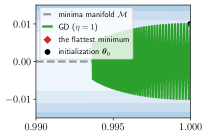
(a) GD with $\eta=1$.

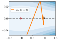
(b) GD with $\eta=2$.

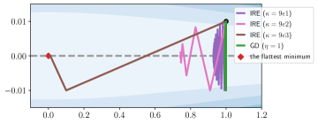
(c) IRE with various $\kappa$’s v.s. GD with $\eta=1$.

Figure 1: A $2$-d example of (1): $\mathcal{L}(u,v)=(1+u^{2})v^{2}/2$. The gray arrows denote to the minima manifold $\mathcal{M}=\{(u,v):v=0\}$, where the smaller the $|u|$, the flatter the minimizer. The red marker highlights the flattest minimizer $(0,0)$. (a) The dynamics of GD ($\eta=1$), which moves slowly towards flatter minima as it converges. (b) The dynamics of GD ($\eta=2$), which diverges due to the excessively large $\eta$. (c) The behavior of our IRE approach with varying $\kappa$’s v.s. GD ($\eta=1$). Is is shown that IRE can significantly accelerate the $u_{t}$’s dynamics, almost reaching the flattest minimum $(0,0)$ when taking a very large $\kappa$.

Accelerating the sharpness reduction.

Inspired by the above analysis, we can accelerate the sharpness reduction by speeding up the flat directions’ dynamics. To this end, there are two approaches:

• Naively increasing the global learning rate $\eta$ (fail). Increasing $\eta$ accelerates the dynamics of $\bm{u}_{t}$, but the largest allowed $\eta$ is constrained by curvatures of sharpest directions. In GD (2), to maintain training stability, $\eta$ must be smaller than $2/\max_{i}\lambda_{i}(\bm{u}_{t})$. Otherwise, $\bm{v}_{t}$’s dynamics will blow up. As illustrated in Figure 1b, setting $\eta=2$ leads to divergence, whereas $\eta=1$ ensures convergence.

• Increasing only the flat directions’ learning rate (our approach, IRE). Specifically, for GD (2), the GD-IRE dynamics is given by

  $$\bm{u}_{t+1} =\bm{u}_{t}-{\color[rgb]{.5,0,.5}{(1+\kappa)}}\frac{\eta}{2}\sum_{i=1}^{m}v_{t,i}^{2}\nabla\lambda_{i}(\bm{u}_{t}),$$ (3)

  $$\bm{v}_{t+1} =(\mathbf{1}-\eta\bm{\lambda}(\bm{u}_{t}))\odot\bm{v}_{t},$$

  where $\kappa>0$ controls the enhancement strength. In GD-IRE (3), $\bm{u}_{t}$’s dynamics is $(1+\kappa)$ faster than that of GD (2). Notably, the sharp directions’ dynamics ($\bm{v}_{t}$) are unchanged. The choice of $\kappa$ only needs to maintain the stability of flat directions’ dynamics, for which, we can always take a significantly large $\kappa$ to enhance the sharpness regularization. As demonstrated in Figure 1c, IRE with larger $\kappa$ always find flatter minima.

Remark 2.2 (The generality).

It is worth noting that similar implicit sharpness regularization also holds for SGD (Ma et al., 2022; Li et al., 2022) and SAM (Wen et al., 2023a). In this section, we focus on the above toy model and GD mainly for illustration. In Appendix A, we provide an analogous illustrative analysis of how IRE accelerates the sharpness reduction of SGD. In Section 5, we further provide theoretical evidence to show that IRE can boost the implicit sharpness regularization of SAM.

3 A Practical Framework of Implementing IRE

Although the preceding illustration of IRE is for GD, in practice, we can incorporate IRE with any base optimizers. Specifically, for a generic update: $\bm{\theta}_{t+1}=\bm{\theta}_{t}-\eta\bm{g}_{t}$, the corresponding IRE modification is given by

$$\bm{\theta}_{t+1}=\bm{\theta}_{t}-\eta(\bm{g}_{t}+\kappa\mathcal{P}_{t}\bm{g}_{t}),$$ (4)

where $\kappa$ denotes the enhancement strength and $\mathcal{P}_{t}:\mathbb{R}^{p}\to\mathbb{R}^{p}$ projects $\bm{g}_{t}$ into the flat directions of the landscape. The flat directions and corresponding projection operator $\mathcal{P}_{t}$ can be estimated using the Hessian information.

However, estimating the full Hessian matrix $\nabla^{2}\mathcal{L}(\bm{\theta}_{t})\in\mathbb{R}^{p\times p}$ is computationally infeasible. Consequently, we propose to use only the diagonal Hessian $\operatorname{diag}(\nabla^{2}\mathcal{L}(\bm{\theta}_{t}))\in\mathbb{R}^{p}$ to estimate $\mathcal{P}_{t}$. Let $\bm{h}_{t}\in\mathbb{R}^{p}$ be an estimate of the diagonal Hessian. Then, we perform the projection as follows

$$\mathcal{P}_{t}\bm{g}_{t} =\bm{n}_{t}\odot\bm{g}_{t},\text{ with }(\bm{n}_{t})_{i}=\begin{cases}1&\text{ if }(|\bm{h}_{t}|)_{i}\leqslant\texttt{Top}_{\rm small}(|\bm{h}_{t}|,\gamma)\\ 0&\text{ otherwise }\end{cases},$$ (5)

where $\gamma\in(0,1)$ and $\texttt{Top}_{\rm small}(|\bm{h}_{t}|,\gamma)$ returns the $\lfloor p\cdot\gamma\rfloor$-th smallest value in $|\bm{h}_{t}|$. Note that $\bm{n}_{t}\in\mathbb{R}^{p}$ denotes a mask vector and the above approximate projection essentially masks the top-$(1-\gamma)$ sharp coordinates out. As such, the projection (5) will retain the top-$\gamma$ flat coordinates. Noticing that in DNNs, there are much more flat directions than sharp directions  (Yao et al., 2020), we thus often use $\gamma>0.5$ in practice.

Input: $\bm{\theta}_{0}$, $T$, $K$, learning rate $\{\eta_{t}\}_{t}$, warm-up time $T_{\rm w}$, ​IRE hyperparams: $\kappa\geqslant 0$ and $\gamma\in(0.5,1)$​;

for $t=T_{\rm w},\cdots,T-1$ do

       Compute the original update direction $\bm{g}_{t}$ according to the base optimizer;

       if $(t-T_{\rm w})\!\!\mod K=0$ then

             Estimate the diagonal Hessian $\bm{h}_{t}\in\mathbb{R}^{p}$ using Eq. (6);

             Update the mask $\bm{n}_{t}\in\mathbb{R}^{p}$ using Eq. (5);

      else

            $\bm{n}_{t}=\bm{n}_{t-1}$

      $\bm{\theta}_{t+1}=\bm{\theta}_{t}-\eta_{t}\big{(}\bm{g}_{t}+$$\kappa\bm{n}_{t}\odot\bm{g}_{t}$$\big{)}$;

Output: $\bm{\theta}_{T}$.

Algorithm 1 Practical IRE (A practical framework of implementing IRE)

A light-weight estimator of the diagonal Hessian. Let $\ell(\cdot,\cdot)$ be the cross-entropy loss. Given an input data $\bm{x}\in\mathbb{R}^{d_{x}}$ and label $\bm{y}\in\mathbb{R}^{d_{y}}$, let the model’s prediction be $f(\bm{x};\bm{\theta})\in\mathbb{R}^{d_{y}}$. The Fisher (Gauss-Newton) matrix $F(\bm{\theta})$ is widely acknowledged to be a good approximation of the Hessian, particularly near minima. Thus, we can estimate the diagonal Hessian by $\bm{h}_{t}={\rm diag}(F(\bm{\theta}_{t}))$, which has been widely used in deep learning optimization (Martens and Grosse, 2015; Grosse and Martens, 2016; George et al., 2018; Mi et al., 2022; Liu et al., 2024). Given an input batch $\{(\bm{x}_{b},\bm{y}_{b})\}_{b=1}^{B}$, the empirical diagonal Fisher is given by ${\rm diag}(\hat{F}(\bm{\theta}))=\frac{1}{B}\sum_{b=1}^{B}\nabla\ell(f(\bm{x}_{b};\bm{\theta});\hat{\bm{y}}_{b})\odot\nabla\ell(f(\bm{x}_{b};\bm{\theta});\hat{\bm{y}}_{b}),\text{ where }\hat{\bm{y}}_{b}\sim{\rm softmax}(f(\bm{\theta};\bm{x}_{b})).$ However, as noted by Liu et al. (2024), implementing this estimator is computationally expensive due to the need to calculate $B$ single-batch gradients. Liu et al. (2024) proposed a more convenient estimator ${\rm diag}(\hat{F}_{\rm eff}(\bm{\theta}))$, only requires computing the mini-batch gradient $\nabla\hat{\mathcal{L}}_{B}(\bm{\theta})=\frac{1}{B}\sum_{b=1}^{B}\nabla\ell(f(\bm{x}_{b};\bm{\theta});\hat{\bm{y}}_{b})\text{ with }\hat{\bm{y}}_{b}\sim{\rm softmax}(f(\bm{x}_{b};\bm{\theta}))$:

$$\bm{h}_{t}={\rm diag}(\hat{F}_{\rm eff}(\bm{\theta}))=B\cdot\nabla\hat{\mathcal{L}}_{B}(\bm{\theta})\odot\nabla\hat{\mathcal{L}}_{B}(\bm{\theta}).$$ (6)

According to Liu et al. (2024), this estimator is an unbiased estimate of the empirical diagonal Fisher, i.e., $\mathbb{E}_{\hat{\bm{y}}}[{\rm diag}(\hat{F}_{\rm eff}(\bm{\theta}))]=\mathbb{E}_{\hat{\bm{y}}}[{\rm diag}(\hat{F}(\bm{\theta}))]$. For more discussions on the efficiency of this estimator, please refer to (Liu et al., 2024, Section 2). Additionally, for squared loss, one can simply use Fisher as the estimator (Liu et al., 2024).

The practical IRE and computational efficiency. The practical IRE is summarized in Algorithm 1, which is notably lightweight. The estimation of $\bm{h}_{t}$ using (6) requires computational resources roughly equivalent to one back-propagation. Consequently, by setting $K=10$ in Algorithm 1 (estimating the projection every 10 steps), the average per-step computational load of IRE is only $1.1$ times that of the base optimizer. This claim can be empirically validated as shown in Table 5.

4 Experiments

In this section, we evaluate how IRE performs when incorporating with various base optimizers. Specifically, we examine the incorporation of IRE with SGD (SGD-IRE), SAM (SAM-IRE), and AdamW (AdmIRE) across vision and language tasks.

4.1 Image classification

4.1.1 Validating our motivation

To show that IRE can accelerate the sharpness reduction, we train WideResNet-16-8 (Zagoruyko and Komodakis, 2016) on CIFAR-10 dataset (Krizhevsky and Hinton, 2009) by SAM-IRE (with $K=10$, varying $\kappa$ and $\gamma$). Here, we incoporate IRE into SAM starting from the $30$-th epochs. We vary $\gamma\in\{0.8,0.9,0.95\}$ and $\kappa\in\{0,2,5,10\}$. Regarding the learning rate (LR), both constant LR and decayed LR are considered. The sharpness is measured by $\operatorname{Tr}(\nabla^{2}\mathcal{L}(\bm{\theta}))$. Further experimental details can be found in Appendix B.

As depicted in Fig. 2(a), SAM-IRE (with constant LR) consistently finds flatter solutions compared to SAM and higher $\kappa$ always leads to flatter minima. Additionally, SAM-IRE also shows robustness to variations of $\gamma$. For SAM-IRE with decayed LR (Fig. 2(b)), SAM-IRE still consistently finds flatter solutions than SAM. Notably, flatter solutions correlate positively with lower training loss and higher test accuracy (Fig. 2(c,d)).

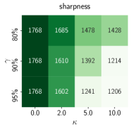
(a) sharpness, constant LR.

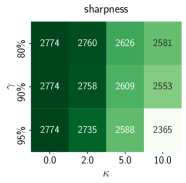
(b) sharpness, decayed LR.

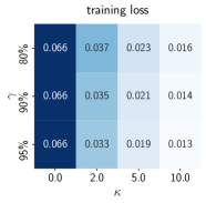
(c) train loss, decayed LR.

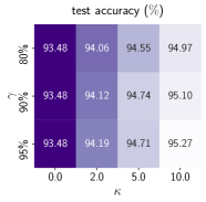
(d) test acc, decayed LR.

Figure 2: Training WRN-16-8 on CIFAR-10 by SAM-IRE with varying $\gamma,\kappa$. Particularly, the case of $\kappa=0$ correspond to the standard SAM.

4.1.2 IRE can consistently improve generalization

Convolutional Neural Networks (CNNs). In this experiment, we first consider the classification of CIFAR-{10,100} with WideResNet-28-10 (Zagoruyko and Komodakis, 2016) and ResNet-56 (He et al., 2016). Both SGD and SAM optimizers are adopted. All the experiments use base data augmentation and label smoothing. For SGD-IRE/SAM-IRE, we fix $K=10$, and tune hyperparameters $\gamma$ and $\kappa$ via a grid search over $\gamma\in\{0.99,0.9,0.8\}$ and $\kappa\in\{1,2\}$. The total epochs are set to 100 for CIFAR-10 and 200 for CIFAR-100, and we switch from SGD/SAM to SGD-IRE/SAM-IRE when the training loss approaches 0.1. The other experimental details are deferred to Appendix B and the results are shown in Table 1.

Secondly, we evaluate IRE for training ResNet-50 on ImageNet (Deng et al., 2009). The experimental details are deferred to Appendix B and the results are shown in Table 3.

Vision Transformers (ViTs). We also examine the impact of IRE on generalization of ViT-T and ViT-S (Dosovitskiy et al., 2020) on CIFAR100. The default optimizers used are AdamW and SAM (Mueller et al., 2024). Strong data augmentations (basic + AutoAugment) are utilized. The total epochs are set to $200$ and we switch from AdamW/SAM to AdmIRE/SAM-IRE when the training loss approaches $0.5$. For AdmIRE/SAM-IRE, we fix $K=10$, and tune hyperparameters $\gamma$ and $\kappa$ via a grid search over $\gamma\in\{0.99,0.9,0.8\}$ and $\kappa\in\{20,50\}$. Other experimental details are deferred to Appendix B. The results are shown in Table 3.

As demonstrated in Table 1, 3 and 3, IRE consistently improves generalization of SGD, AdamW and SAM across all settings examined.

Table 1: WRN-28-10/ResNet-56 on CIFAR-10/100.

	WRN-28-10		ResNet-56
	CIFAR-10	CIFAR-100	CIFAR-10	CIFAR-100
SGD	95.84	80.81	93.49	72.81
SGD-IRE	96.24 (+0.40)	81.49 (+0.68)	93.78 (+0.29)	73.78 (+0.97)
SAM	96.58	83.05	94.05	75.54
SAM-IRE	96.70 (+0.12)	83.50 (+0.45)	94.46 (+0.41)	75.86 (+0.32)

Table 2: ResNet-50 on ImageNet.

	Top-1	Top-5
SGD	76.81	93.31
SGD-IRE	77.04 (+0.23)	93.58 (+0.27)
SAM	77.47	93.90
SAM-IRE	77.92 (+0.45)	94.12 (+0.22)

Table 3: ViT-T/S on CIFAR-100.

	ViT-T	ViT-S
AdamW	63.90	65.43
AdmIRE	67.05 (+3.15)	68.39 (+2.96)
SAM	64.25	66.93
SAM-IRE	67.33 (+3.08)	70.47 (+3.54)

4.2 Large language model pre-training

We now evaluate IRE in the pre-training of decoder-only large language models (LLMs). Following the training protocol of Llama models, we employ the AdamW optimizer with hyperparameters $\beta_{1}=0.9,\beta_{2}=0.95$ and weight decay $\lambda=0.1$ (Touvron et al., 2023). The learning rate strategy includes a warm-up phase followed by a cosine decay scheduler, capped at lr_max. In each experiment, we tune lr_max only for AdamW and use it also for AdmIRE, for which the IRE is activated at the end of warm-up phase.

4.2.1 Computational efficiency and hyperparameter robustness

The first experiment is conducted to verify both the computational efficiency and the robustness of hyperparameters ($\gamma,\kappa$) in IRE for pre-training tasks. Specifically, we train a 2-layer decoder-only Transformer (8M) on the Wikitext-2 dataset (4.3M) (Merity et al., 2016) by AdamW and AdmIRE (with $K=10$ and varying $\gamma,\kappa$). The total training duration is 100k steps, including a 3k-step warm-up phase.

Table 4: Wall-clock time on 1 A800.

Algorithm	time (/step)
AdamW	0.165s
AamIRE	0.185s

Table 5: Transformer on wikitext-2.

First, we tune lr_max in AdamW, identifying the optimal lr_max=6e-4. Subsequently, we train both AdamW and AdmIRE using this lr_max.

Computational efficiency.

As shown in Table 5, AdmIRE with $K=10$ (estimating the projection mask every 10 steps) is computationally efficient: the average time per step of AdmIRE is only $1.12$ times that of AdamW, corresponding to the theoretical estimation ($1.1$ times).

Robustness to hyperparameters.

Fig. 5 shows that AdmIRE, with varying $\gamma$ and $\kappa$, consistently speeds up the pre-training. Remarkably, with the best configuration, AdmIRE can achieves 5.4$\times$ speedup than well-tuned AdamW.

More experimental details and results are deferred to Appendix B.

4.2.2 Experiments on Llama models

Llama (Touvron et al., 2023), a popular open LLM, exhibits remarkable capabilities across general domains. In this section, we examine the performance of AdmIRE in training Llama models of various sizes across various datasets:

• Llama (60M) on wikitext-103 (0.5G). Wikitext-103 (Merity et al., 2016) serves as a standard language modeling benchmark for pre-training, which contains 103M training tokens from 28K articles, with an average length of 3.6K tokens per article.

• Llama (119M) on minipile (6G). Minipile (Kaddour, 2023), a 6GB subset of the deduplicated Pile (825GB) (Gao et al., 2020) presents a highly diverse text corpus. Given its diversity, training on minipile poses more challenges and potential instabilities for optimizers compared to Wikitext-103.

• Llama (229M) on openwebtext (38G). Openwebtext (Gokaslan and Cohen, 2019), an open-source recreation of the WebText corpus, is extensively utilized for LLM pre-training such as RoBERTa (Liu et al., 2019b) and GPT-2 (Radford et al., 2019).

Additionally, gradient clipping is adopted to maintain the training stability (Pascanu et al., 2012). First, we tune lr_max in AdamW for each of the three experiments, separately. The optimal lr_max identified for these three experiments is all 6e-4. Then, both AdamW and AdmIRE are trained using this optimal lr_max. For more details, please refer to Appendix B.

AdmIRE is $2\times$ faster than AdamW. The results are reported in Figure 3. We can see that AdmIRE consistently achieves a $2.1\times$ speedup compared with well-tuned AdamW for all three cases. However, the underlying mechanism remains unclear and is left for future work.

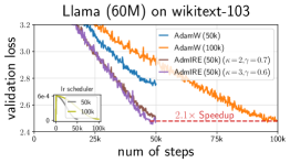
(a)

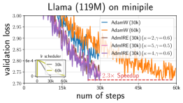
(b)

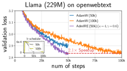
(c)

Figure 3: AdmIRE outperforms AdamW in the pre-training of Llama models.

5 Theoretical Guarantees for IRE on SAMs

Both empirical (Foret et al., 2021) and theoretical (Wen et al., 2023a) studies have validated that SAM algorithms exhibit superior sharpness regularization compared to (S)GD. In this section, we provide a theoretical analysis demonstrating that IRE can further enhance the sharpness regularization of SAM algorithms substantially.

5.1 Theoretical setups

Recall that $\mathcal{L}(\bm{\theta}):=\frac{1}{n}\sum_{i=1}^{n}\mathcal{L}_{i}(\bm{\theta})$ denote the total loss, where $\mathcal{L}_{i}(\bm{\theta})$ is the loss on the $i$-th data. Without loss of generality, we assume $\min_{\bm{\theta}}\mathcal{L}(\bm{\theta})=0$. We further make the following assumption:

Assumption 5.1 (Manifold of minimizers).

Assume that $\mathcal{L}\in\mathcal{C}^{4}(\mathbb{R}^{p})$, $\mathcal{M}:=\operatorname*{arg\,min}_{\bm{\theta}}\mathcal{L}(\bm{\theta})$ is a ($p-m$)-dim $\mathcal{C}^{2}$-submanifold in $\mathbb{R}^{p}$ for some $m\in[p]$, and $\mathrm{rank}(\nabla^{2}\mathcal{L}(\bm{\theta}))=m$ for any $\bm{\theta}\in\mathcal{M}$.

The above connectivity assumption on the manifold of minimizers $\mathcal{M}$ has been empirically verified in works such as Draxler et al. (2018) and Garipov et al. (2018), and theoretically supported in Cooper (2018). This assumption is also widely used in the theoretical analysis of implicit regularization (Fehrman et al., 2020; Li et al., 2022; Arora et al., 2022; Wen et al., 2023a).

Besides, we introduce the following definitions to characterize the dynamics of gradient flow (GF) near the minima manifold $\mathcal{M}$, which is also used in the related works above.

Definition 5.2 (Limiting map of GF).

Consider the GF: $\frac{{\textnormal{d}}\bm{\theta}(t)}{{\textnormal{d}}t}=-\nabla\mathcal{L}(\bm{\theta}(t))$ starting from $\bm{\theta}(0)=\bm{\theta}$. Denote by $\Phi(\bm{\theta}):=\lim_{t\to\infty}\bm{\theta}(t)$ the limiting map of this GF.

Definition 5.3 (Attraction set of $\mathcal{M}$).

Let $U$ be the attraction set of $\mathcal{M}$ under GF, i.e., GF starting in $U$ converges to some point in $\mathcal{M}$. Formally, $U:=\{\bm{\theta}\in\mathbb{R}^{p}:\Phi(\bm{\theta})\in\mathcal{M}\}$.

As proven in (Arora et al., 2022, Lemma B.15), Assumption 5.1 ensures that $U$ (in Definition 5.3) is open and $\Phi(\cdot)$ (in Definition 5.2) is $\mathcal{C}^{2}$ on $U$.

5.2 Theoretical results

The stochastic SAM (Foret et al., 2021) is given by

$$\text{standard SAM:}\quad\bm{\theta}_{t+1}=\bm{\theta}_{t}-\eta\nabla\mathcal{L}_{i_{t}}\left(\bm{\theta}_{t}+\rho\frac{\nabla\mathcal{L}_{i_{t}}(\bm{\theta}_{t})}{\left\|\nabla\mathcal{L}_{i_{t}}(\bm{\theta}_{t})\right\|}\right),\text{ where }i_{t}\sim\mathbb{U}([n]).$$ (7)

The generalization capability of standard SAM can be bounded by the average sharpness, $\mathcal{L}^{\rm avg}(\bm{\theta}):=\mathbb{E}_{\bm{\xi}\sim\mathcal{N}(\mathbf{0},I)}\mathcal{L}\left(\bm{\theta}+\rho{\bm{\xi}}/{\left\|\bm{\xi}\right\|}\right)$ (Foret et al., 2021). This leads researchers to also explore average SAM (Wen et al., 2023a; Zhu et al., 2023; Ujváry et al., 2022), which minimizes $\mathcal{L}^{\rm avg}$:

$$\text{average SAM:}\quad\bm{\theta}_{t+1}=\bm{\theta}_{t}-\eta\nabla\mathcal{L}\left(\bm{\theta}_{t}+\rho{\bm{\xi}_{t}}/{\left\|\bm{\xi}_{t}\right\|}\right),\text{ where }\bm{\xi}_{t}\sim\mathcal{N}(\mathbf{0},I).$$ (8)

Two-phase algorithms. Our theoretical focus is on how IRE accelerates the sharpness reduction of SAM (7) and (8) near the minima manifold $\mathcal{M}$. Thus, we analyze the two-phase algorithms. Specifically, let the initialization $\bm{\theta}_{0}\in U$. In Phase I ($t\leqslant T_{\rm I}$), we employ GF $\frac{{\textnormal{d}}\bm{\theta}_{t}}{{\textnormal{d}}t}=-\nabla\mathcal{L}(\bm{\theta}_{t})$ to ensure that the loss decreases sufficiently; then in Phase II ($T_{\rm I}<t\leqslant T_{\rm I}+T_{\rm II}:=T$), we incorporate IRE into the standard / average SAM.

Effective dynamics: sharpness regularization. The implicit regularization of SAMs can be modeled using effective dynamics. In Phase II, $\bm{\theta}_{t}$ are close the manifold of minimizers $\mathcal{M}$ and let $\bm{z}_{t}:=\Phi(\bm{\theta}_{t})\in\mathcal{M}$. Then, the effective dynamics is given by $\{\bm{z}_{t}\}_{t=T_{\rm I}+1}^{T}$, revealing how SAMs explore the manifold of minimizers $\mathcal{M}$. Particularly, Wen et al. (2023a) showed that the effective dynamics of standard/average SAM are both

$$\mathbb{E}\left[\bm{z}_{t+1}\right]=\bm{z}_{t}-\eta_{\rm eff}\nabla_{\mathcal{M}}\mathrm{Tr}\left[\nabla^{2}\mathcal{L}(\bm{z}_{t})/2\right]+o(\eta_{\rm eff}),$$ (9)

which minimizes the trace of Hessian on $\mathcal{M}$. The difference between the standard SAM (7) and average SAM (8) lies in the effective learning rate (LR) $\eta_{\rm eff}$’s. A visual illustration of some quantities in (9) is provided in the figure above.

Summary of our theoretical results. In this section, we show that incorporating IRE into SAMs can significantly increase the effective LR $\eta_{\rm eff}$ in (9) while maintaining the same training stability as SAMs. In Table 6, we present the effective LR for SAMs and the SAM-IREs. We see clearly that IRE can accelerate the sharpness reduction by a non-trivial factor for both standard and average SAM.

Table 6: Comparison of the implicit regularization strength of SAMs w/o IRE.

Algorithm	Effective LR: $\eta_{\rm eff}$
average SAM (8)	$\eta^{2}/p$ (Thm 5.5)
IRE + average SAM (8)	$\eta^{1.5}/p$ (Thm 5.5)
standard SAM (7)	$\eta\rho^{2}$ (Thm 5.6; Wen et al. (2023a))
IRE + standard SAM (7)	$\eta\rho$ (Thm 5.6)

Remark 5.4 (The mechanism of IRE’s success).

The success of SAM-IRE follows the same mechanism illustrated in Section 2. The key fact that IRE only increases the LR along flat directions has two implications: 1) It does not change the trend of implicit regularization in Eq. (9) but accelerates SAMs’ effective dynamics by a factor of $(1+\kappa)$; 2) Since the LR is only increased along flat directions, $\kappa$ can be set substantially large without hurting the training stability, because the dynamics in sharp directions remain unchanged. Specifically, we theoretically justify in SAM-IRE, $\kappa$ can be selected as large as $1/\rho$.

5.2.1 IRE on average SAM: An $\Omega(1/\eta^{0.5})$ acceleration

We first consider IRE on average SAM. Let $T_{\rm I}$ be the hitting time: $T_{\rm I}:=\inf\{t\geqslant 0:\left\|\bm{\theta}_{t}-\Phi(\bm{\theta}_{t})\right\|=\mathcal{O}(\sqrt{\eta}\rho)\}$. When running GF in Phase I, Definition 5.3 guarantees $T_{\rm I}<\infty$. Thus, at the starting of Phase II, $\left\|\bm{\theta}_{t}-\Phi(\bm{\theta}_{t})\right\|=\mathcal{O}(\sqrt{\eta}\rho)$. Furthermore, the following result holds for Phase II.

Theorem 5.5 (IRE on average SAM).

Suppose Assumption 5.1 holds. If $\eta=\mathcal{O}(1)$ and $\rho=\mathcal{O}(\sqrt{\eta})$ in SAM (8), ​$\kappa\leqslant 1/\rho$​, and $\mathcal{P}_{t}=P_{m+1:p}(\nabla^{2}\mathcal{L}(\bm{\theta}_{t}))$ in IRE (4), then with high probability at least $1-T_{\rm II}^{2}\exp\left(-\Omega\left(1/\left(\eta+p^{-1}\right)\right)\right)$, $\left\|\bm{\theta}_{t}-\Phi(\bm{\theta}_{t})\right\|=\mathcal{O}(\sqrt{\eta}\rho)$ holds for all $T_{\rm I}\leqslant t\leqslant T$. Furthermore, the effective dynamics of $\bm{z}_{t}:=\Phi(\bm{\theta}_{t})\in\mathcal{M}$ satisfies:

$$\mathbb{E}_{\bm{\xi}_{t}}[\bm{z}_{t+1}]=\bm{z}_{t}-\frac{{\color[rgb]{.5,0,.5}(1+\kappa)}\eta\rho^{2}}{p}\nabla_{\mathcal{M}}\operatorname{Tr}\left[\nabla^{2}\mathcal{L}(\bm{z}_{t})/2\right]+\mathcal{O}(\eta^{3/2}\rho^{2}).$$

Note that $\rho=\mathcal{O}(\sqrt{\eta})$ and $\kappa$ can be as large as $1/\rho$. Consequently, the effective LR of minimizing the trace of Hessian can be selected as large as $\eta_{\rm eff}=(\kappa+1)\eta\rho^{2}/p=\mathcal{O}(\eta^{1.5}/p)$. In contrast, that of average SAM is at most $\mathcal{O}(\eta^{2}/p)$. The proof of Theorem 5.5 can be found in Appendix C.

5.2.2 IRE on standard SAM: An $\Omega(1/\rho)$ acceleration

This subsection delves into IRE on standard SAM (7), which is more widely used and often yields better performance than average SAM (8). However, since standard SAM (7) requires stochastic gradients $\nabla\mathcal{L}_{i}(\bm{\theta})$ ($i\in[n]$), we need an additional assumption regarding the features on the manifold (see Setting D.1), which is commonly used in the literature (Du et al., 2018; 2019; Li et al., 2022; Arora et al., 2022; Wen et al., 2023a). We defer it to Appendix D due to space constraints. Under this Setting, Assumption 5.1 holds naturally with $m=n$.

During Phase I of GF, Definition 5.3 ensures that there exists $t<\infty$ such that $\left\|\bm{\theta}_{t}-\Phi(\bm{\theta}_{t})\right\|=\mathcal{O}(\eta^{1-\alpha}\rho)$ for any $\alpha\in[0,1)$. We define $T_{\rm I}$ as the hitting time: $T_{\rm I}:=\inf\{t\geqslant 0:\left\|\bm{\theta}_{t}-\Phi(\bm{\theta}_{t})\right\|=\mathcal{O}(\eta^{1-\alpha}\rho)\}$. Then the following result holds for Phase II, whose proof can be founded in Appendix D.

Theorem 5.6 (IRE on standard SAM).

Under Setting D.1, if $\eta,\rho=\mathcal{O}(1)$ in SAM (7), ​$\kappa\leqslant 1/\rho$​, and $\mathcal{P}_{t}=P_{n+1:p}(\nabla^{2}\mathcal{L}(\bm{\theta}_{t}))$ in IRE (4), then with high probability at least $1-T_{\rm II}^{2}\exp\left(-\Omega(1/\eta^{\alpha})\right)$, $\left\|\bm{\theta}_{t}-\Phi(\bm{\theta}_{t})\right\|=\mathcal{O}(\eta^{1-\alpha}\rho)$ holds for all $T_{\rm I}\leqslant t\leqslant T$. Moreover, the effective dynamics $\bm{z}_{t}=\Phi(\bm{\theta}_{t})\in\mathcal{M}$ satisfies:

$$\mathbb{E}_{i_{t}}[\bm{z}_{t+1}]=\bm{z}_{t}-{\color[rgb]{.5,0,.5}(1+\kappa)}\eta\rho^{2}\nabla_{\mathcal{M}}\operatorname{Tr}\left[\nabla^{2}\mathcal{L}(\bm{z}_{t})/2\right]+\mathcal{O}\left((\kappa+1)\eta\rho^{2}(\rho+\eta^{1-\alpha})\right).$$

Taking $\kappa=0$ and $\alpha=0$ recovers the result established in Wen et al. (2023a). However, $\kappa$ can be as large as $1/\rho$, where IRE provides a $\Theta(1/\rho)$-time acceleration over the standard SAM.

6 Conclusion

In this work, we propose a novel IRE framework to enhance the implicit sharpness regularization of base optimizers. Experiments demonstrate that IRE not only consistently improves generalization but also accelerates loss convergence in the pre-training of Llama models of various sizes. For future work, there are two urgent directions: 1) understanding why IRE can accelerate convergence, which may require studying the interplay between IRE and the Edge of Stability (EoS) (Wu et al., 2018; Jastrzębski et al., 2017; Cohen et al., 2021); and 2) conducting a larger-scale investigation into the acceleration of AdmIRE compared to AdamW in LLM pre-training, as well as the downstream performance of the LLMs pre-trained by AdmIRE.

  Appendix  

[sections] [sections]l1

Appendix A Proofs for SGD in Section 2

For the example in Section 2, we have studied the implicit sharpness regularization of GD dynamics and how IRE enhances the implicit regularization of GD. In this Section, we illustrate that, for this example, similar results hold for SGD dynamics.

SDE Modelling of SGD. We consider SGD approximated by SDE (Li et al., 2017; 2019; 2022) with noise covariance $\Sigma$: ${\textnormal{d}}\bm{\theta}_{t}=-\nabla\mathcal{L}(\bm{\theta}_{t}){\textnormal{d}}t+\sqrt{\eta\Sigma(\bm{\theta}_{t})}{\textnormal{d}}W_{t}$. We consider that the noise covariance aligns with the Hessian near minima, i.e., $\Sigma(\bm{\theta})=\begin{pmatrix}\mathbf{0}_{d}&0\\ 0&\sigma^{2}h(\bm{u})\end{pmatrix}$ (where $\sigma>0$ is a scalar), such as the label noise (Damian et al., 2021; Li et al., 2022). Then, the SDE above can be rewritten as

$${\textnormal{d}}\begin{pmatrix}\bm{u}_{t}\\ v_{t}\end{pmatrix}=-\begin{pmatrix}v_{t}^{2}\nabla h(\bm{u}_{t})/2\\ v_{t}h(\bm{u}_{t})\end{pmatrix}{\textnormal{d}}t+\begin{pmatrix}0\\ \sqrt{\eta\sigma^{2}h(\bm{u}_{t})}{\textnormal{d}}W_{t}\end{pmatrix}.$$ (10)

Implicit Sharpness Regularization. Intuitively, when $v_{t}$ is close to $0$, the speed of $\bm{u}_{t}$ is much slower than $v_{t}$ due to $v_{t}^{2}\ll v_{t}$. Following Ma et al. (2022), when this speed separation is large, $v_{t}$ is always at equilibrium given $\bm{u}_{t}$. Solving the Ornstein–Uhlenbeck process about $v_{t}$, we know the equilibrium distribution of $v_{t}$ is $v_{\infty}\sim\mathcal{N}(0,\eta\sigma^{2})$, and hence the dynamics $\bm{u}_{t}$ (along the manifold) is

$${\textnormal{d}}\bm{u}_{t}/{\textnormal{d}}t=-\mathbb{E}_{v_{\infty}}\left[{v_{\infty}^{2}\nabla h(\bm{u}_{t})/2}\right]=-\nabla h(\bm{u}_{t})/2.$$ (11)

This derivation clearly shows the slow “effective dynamics” $\bm{u}_{t}$ along the manifold is a gradient flow minimizing the sharpness $h(\cdot)$. When SGD minimizes the loss, it also minimzes the sharpness implicitly, that is to say, SGD has the following implicit sharpness regularization: $\min_{\bm{\theta}}\operatorname{Tr}(\nabla^{2}\mathcal{L}(\bm{\theta}))\ {\rm s.t.\mathcal{L}(\bm{\theta})\approx 0}$.

Generalization and Optimization benefits of the sharpness regularization. In terms of generalization, as discussed in related works, a common view is that flat minima generalize well, which has been proved in a large number of previous works. In addition, in terms of optimization, after SGD reaches the equilibrium $v_{\infty}\sim\mathcal{N}(0,\eta\sigma^{2})$, the loss near the flat minimum is smaller because $\mathbb{E}_{v_{\infty}}[\mathcal{L}(\bm{\theta})]=\mathbb{E}_{v_{\infty}}[h(\bm{u})v_{\infty}^{2}/2]=\eta\sigma^{2}h(\bm{u})/2\propto\operatorname{Tr}(\nabla^{2}\mathcal{L}(\bm{u}))$.

Q. How can we enhance the implicit sharpness regularization of SGD?
A. Accelerating SGD’s slow “effective dynamics” $\bm{u}_{t}$ along the minima manifold.

Implicit Regularization Enhancement (IRE) by accelerating the effective dynamics along minima manifold. First, it is worth noting that naively increasing the learning rate $\eta$ cannot achieve our aim, because increasing $\eta$ will influence the dynamic stability of $v_{t}$ and the equilibrium $v_{\infty}$. Therefore, we need to accelerate the effective dynamics $\bm{u}_{t}$ without affecting the dynamics of $v_{t}$. Another main point is that SGD’s effective dynamics $\bm{u}_{t}$ can naturally minimize the sharpness implicitly, so we only need to enhance this property. To achieve this, we only need to correct the update direction in (10) from $-\nabla\mathcal{L}(\bm{\theta}_{t})$ to $-(\nabla\mathcal{L}(\bm{\theta}_{t})+{\color[rgb]{.5,0,.5}{\kappa P_{\mathcal{M}}\nabla\mathcal{L}(\bm{\theta}_{t}))}}$, where $P_{\mathcal{M}}$ is the projection matrix to the manifold $\mathcal{M}$ and $\kappa$ is a scalar. Using this new algorithm, the SDE dynamics corresponds to

$${\textnormal{d}}\begin{pmatrix}\bm{u}_{t}\\ v_{t}\end{pmatrix}=-\begin{pmatrix}{\color[rgb]{.5,0,.5}{(1+\kappa)}}v_{t}^{2}\nabla h(\bm{u}_{t})/2\\ v_{t}h(\bm{u}_{t})\end{pmatrix}{\textnormal{d}}t+\begin{pmatrix}0\\ \sqrt{\eta\sigma^{2}h(\bm{u}_{t})}{\textnormal{d}}W_{t}\end{pmatrix}.$$ (12)

Comparing (10) and (12), the dynamics of $v_{t}$ are the same, so they attain the same equilibrium distribution $v_{\infty}\sim\mathcal{N}(0,\eta\sigma^{2})$. As for the effective dynamics along manifold, (10) corresponds to the form:

$${\textnormal{d}}\bm{u}_{t}/{\textnormal{d}}t=-\mathbb{E}_{v_{\infty}}\left[(1+\kappa){v_{\infty}^{2}\nabla h(\bm{u}_{t})/2}\right]=-(1+\kappa)\nabla h(\bm{u}_{t})/2.$$ (13)

$(1+\kappa)$ times Enhancement. Comparing (13) and (11), it is clear that our new algorithm can enhance implicit sharpness regularization $(1+\kappa)$ times faster than the original SGD.

Appendix B Experimental Details

This section describes the experimental details in Section 4.

B.1 Experimental details in Section 4.1

B.1.1 Experimental details in Section 4.1.1

We train WideResNet-16-8 on CIFAR-10 dataset by SAM-IRE (with $K=10$, varying $\kappa$ and $\gamma$). The experiments employ basic data augmentations and 0.1 label smoothing, as outlined by Foret et al. (2021). The mini-batch size is set to 128, the weight decay is set to 5e-4, and the $\rho$ in SAM is to 0.05, as in Foret et al. (2021). To evaluate the implicit flatness regularization of SAM itself, the momentum is set to 0.0. Regarding the learning rate (lr), we evaluate for both constant lr (within our theoretical framework) and decayed lr (common in practice though not covered by our theory). In the experiment in Fig 2 (a), a fixed lr $0.1$ is used. In the experiment in Fig 2 (b)(c)(d), a step-decayed lr schedule is employed, starting at $0.1$ and reducing lr by a factor of $5$ at epoch 20, 50, 80. We transit from SAM to SAM-IRE at the 30th epoch out of 100 total epochs. We test $\gamma$ in $0.8,0.9,0.95$, and $\kappa$ in $0$ (original SAM), $2,5,10$.

The flatness measure, $\operatorname{Tr}(\nabla^{2}\mathcal{L}(\bm{\theta}))$, is approximated by the trace of Fisher $\operatorname{Tr}(\bm{F}(\bm{\theta}))$. Specifically, we use ${\rm diag}(\hat{F}_{\rm eff}(\bm{\theta}))$ in (6) for the estimate because $\mathbb{E}_{\hat{\bm{y}}}[{\rm diag}(\hat{F}_{\rm eff}(\bm{\theta}))]=\mathbb{E}_{\hat{\bm{y}}}[{\rm diag}(\hat{F}(\bm{\theta}))]$ and thus,

$$\operatorname{Tr}(\nabla^{2}\mathcal{L}(\bm{\theta}))\approx\mathbb{E}_{\hat{\bm{y}}}[\operatorname{Tr}(\hat{F}(\bm{\theta}))]=\mathbb{E}_{\hat{\bm{y}}}[\operatorname{Tr}(\operatorname{diag}(\hat{F}(\bm{\theta})))]=\mathbb{E}_{\hat{\bm{y}}}[{\rm diag}(\hat{F}_{\rm eff}(\bm{\theta}))].$$

Moreover, the first “$\approx$” above takes “$=$” when $\mathcal{L}(\bm{\theta})=0$.

B.1.2 Experimental details in Section 4.1.2

Experiments for CNNs on CIFAR-10/CIFAR-100. We first evaluate the impact of IRE on generalization of baseline models (WideResNet-28-10 and ResNet-56) and default optimizers (SGD and SAM) on CIFAR-{10,100}. For the base optimizers, SGD and SAM, cosine learning rate decay is adopted with an initial lr $0.1$. For other training components, we follow the settings in Foret et al. (2021): basic data augmentations and $0.1$ label smoothing; for both SGD and SAM, the momentum is set to $0.9$, the batch size is set to $128$, and the weight decay is set to 5e-4; for SAM, $\rho$ is set to $0.05$ for CIFAR-10 and $0.1$ for CIFAR-100. The total epochs is set to 100 for CIFAR-10 and 200 for CIFAR-100, and we switch from SGD/SAM to SGD-IRE/SAM-IRE when the training loss approaches 0.1. For SGD-IRE/SAM-IRE, we fix $K=10$, and tune hyperparameters $\gamma$ and $\kappa$ via a grid search over $\gamma\in\{0.99,0.9,0.8\}$ and $\kappa\in\{1,2\}$. The results are reported in Table 1.

Experiments without finely tuned hyperparameters. A high sensitivity to the choice of hyperparameters would make a method less practical. To demonstrate that our IRE performs even when $\kappa,\gamma$ are not finely tuned, we conduct experiments using fixed $\gamma=0.99,\kappa=1$, under the same settings as described above.. The results (averaged over 3 random seeds) are reported in Table 7.

Table 7: Results for SGD-IRE and SAM-IRE on {WideResNet-28-10, ResNet-56} on CIFAR-{10, 100}, using fixed $\gamma=0.99,\kappa=1$ in IRE.

	WideResNet-28-10		ResNet-56
	CIFAR-10	CIFAR-100	CIFAR-10	CIFAR-100
SGD	95.93	80.77	93.80	72.72
SGD-IRE	96.13 (+0.20)	81.12 (+0.35)	93.94(+0.14)	72.93(+0.21)
SAM	96.73	83.22	94.58	75.25
SAM-IRE	96.75 (+0.02)	83.40 (+0.19)	94.65 (+0.07)	75.49 (+0.24)

Experiments for CNNs on ImageNet. We also examine the impact of IRE on generalization of ResNet-50 and default optimizers (SGD and SAM) on on ImageNet. Following Foret et al. (2021) and Kwon et al. (2021), we use basic data augmentations and $0.1$ label smoothing. For the base optimizers, SGD and SAM, we also follow the settings in Kwon et al. (2021): the momentum is set to $0.9$; cosine learning rate decay is adopted with an initial lr $0.2$; the batch size is set to 1024; the weight decay is set to 1e-4; for SAM, $\rho$ is set to $0.05$. The total epochs is set to 200, and we switch from SGD/SAM to SGD-IRE/SAM-IRE when the training loss approaches 1.5. For SGD-IRE/SAM-IRE, we fix $K=10$, and tune hyperparameters $\gamma$ and $\kappa$ via a grid search over $\gamma\in\{0.8,0.6\}$ and $\kappa\in\{2,4\}$. The results are reported in Table 3.

Experiments for ViTs on CIFAR-100. We examine the impact of IRE on generalization of ViT-T and ViT-S on CIFAR-100. We follow the settings in Mueller et al. (2024): the default optimizers used are AdamW and SAM, with cosine lr decay to $0$ starting from an initial lr 1e-4; the weight decay is 5e-4; batch size is $64$; strong data augmentations (basic + AutoAugment) are utilized; $\rho=0.1$ for SAM. The total epochs are set to $200$, and we switch from AdamW/SAM to AdmIRE/SAM-IRE when the training loss approaches $0.5$. For AdmIRE/SAM-IRE, we fix $K=10$, and tune hyperparameters $\gamma$ and $\kappa$ via a grid search over $\gamma\in\{0.99,0.9,0.8\}$ and $\kappa\in\{20,50\}$. The results are reported in Table 3.

B.2 Experimental details in Section 4.2

B.2.1 Experimental details in Section 4.2.1

We train a 2-layer decoder-only Transformer (8M parameters) using absolute positional encodings (Vaswani et al., 2017), with 8 heads in each layer and a hidden size of 128, on the wikitext-2 dataset (4.3M) by AdamW and AdmIRE (with $K=10$ and varying $\gamma,\kappa$). The (max) sequence length is set to 512, and the batch size is set to 32. The experiments in this section are conducted on 1 A800.

For the optimizer AdamW, we use the hyperparameters $\beta_{1}=0.9,\beta_{2}=0.95$ and weight decay $\lambda=0.1$, as suggested in Touvron et al. (2023). The total training duration is 100,000 steps, including 3,000 warm-up steps followed by a cosine decay scheduler with lr_max and lr_min=lr_max$/20$.

First, we tune lr_max in AdamW from $\{$1.5e-4, 3e-4, 6e-4, 1.2e-3, 1.8e-3, 3e-3$\}$. The results, shown in Figure 4 (left), identify the optimal lr_max=6e-4. We also use the optimal lr_max of 6e-4 for AdmIRE, for which the IRE is enable at the end of warm-up phase.

The results are reported in Figure 5.

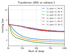
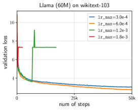
Figure 4: The results for tuning lr_max in AdamW.

B.2.2 Experimental details in Section 4.2.2

Llama (Touvron et al., 2023) is a decode-only Transformer architecture using Rotary Positional Encoding (RoPE) (Su et al., 2024), Swish-Gated Linear Unit (SwiGLU) (Shazeer, 2020), and Root mean square layer normalization (RMSNorm) (Zhang and Sennrich, 2019). The experiments in this section examine the performance of AdmIRE in training Llama models with different sizes. For implementation, we utilize the Llama code available on huggingface. The experiments are conducted on 4 H800.

For the optimizer AdamW, we use the well-tuned hyperparameters $\beta_{1}=0.9,\beta_{2}=0.95$ and weight decay $\lambda=0.1$ for LLama (Touvron et al., 2023). The learning rate strategy integrates a warm-up phase followed by a cosine decay scheduler with lr_max and lr_min=lr_max$/20$. Additionally, it is used with gradient clipping 1.0 to maintain the training stability.

In each experiment, we tune the optimal lr_max for AdamW and then use it also for AdmIRE, for which the IRE is enable at the end of warm-up phase.

Llama (60M) on wikitext-103 (0.5G). We train a 16-layer Llama model, with 10 heads in each layer and a hidden size of 410, on the wikitext-103 dataset. The (max) sequence length is set to 150, and the batch size is set to 240, following Dai et al. (2019). The total training duration is 50,000 or 100,000 steps, including 500 warm-up steps. First, we tune lr_max in AdamW from $\{$3e-4, 6e-4, 1.2e-3, 1.8e-3$\}$, identifying the optimal lr_max 6e-4. The experimental results are very similar to Figure 4 (right), so we will not show them again. Then, both AdamW and AdmIRE are trained using the optimal lr_max.

Llama (119M) on minipile (6G). We train a 6-layer Llama model, with 12 heads in each layer and a hidden size of 768, on the minipile dataset. The (max) sequence length is set to 512, and the batch size is set to 300. The total training duration is 30,000 or 60,000 steps, including 300 warm-up steps. First, we tune lr_max in AdamW from $\{$3e-4, 6e-4, 1.2e-3, 1.8e-3$\}$, identifying the optimal lr_max 6e-4. (The results are very similar to Figure 4 (right), so we do not show them repeatly.) Then, both AdamW and AdmIRE are trained using the optimal lr_max.

Llama (229M) on openwebtext (38G). We train a 16-layer Llama model, with 12 heads in each layer and a hidden size of 768, on the openwebtext dataset. The (max) sequence length is set to 1024, and the batch size is set to 480, following nanoGPT and Liu et al. (2024). The total training duration is 50,000 or 100,000 steps, including 1,000 warm-up steps. First, we tune lr_max in AdamW from $\{$3e-4, 6e-4, 1.2e-3, 1.8e-3$\}$, identifying the optimal lr_max 6e-4. (The results are very similar to Figure 4 (right), so we do not show them repearly.) Then, both AdamW and AdmIRE are trained using the optimal lr_max.

Appendix C Proofs in Section 5.2.1

Additional Notations. For the proofs in Section 5, some additional notations are used. For any set $K\subset\mathbb{R}^{p}$ and a constant $R>0$, we denote $\mathbb{B}(K;R):=\{\bm{\theta}\in\mathbb{R}^{p}:{\rm dist}(\bm{\theta};K)\leqslant R\}$. $\left\langle\cdot,\cdot\right\rangle$ represents the standard Euclidean inner product between two vectors. $\left\|\cdot\right\|$ denotes the $\ell_{2}$ norm of a vector or the spectral norm of a matrix, whereas $\|\cdot\|_{\rm F}$ denotes the Frobenius norm of a matrix.

C.1 Preliminary Lemmas

Lemma C.1 (Arora et al. (2022), Lemma B.2).

Under Assumption 5.1, for any compact set $K\subset\Gamma$, there exist absolute constants $R_{1},\mu>0$ such that

• (i) ${\mathbb{B}(K;R_{1})}\subset U$;

• (ii) $\mathcal{L}(\cdot)$ is $\mu$-PL (defined in Def E.1) on ${\mathbb{B}(K;R_{1})}$;

• (iii) $\inf\limits_{\bm{\theta}\in{\mathbb{B}(K;R_{1})}}\lambda_{m}\left(\nabla^{2}\mathcal{L}(\bm{\theta})\right)\geqslant\mu$.

We further define the following absolute constants on $\mathbb{B}(K;R_{1})$:

$$\beta_{2}:=\sup_{\bm{\theta}\in{\mathbb{B}(K;R_{1})}}\left\|\nabla^{2}\mathcal{L}(\bm{\theta})\right\|;\quad\beta_{3}:=\sup_{\bm{\theta}\in{\mathbb{B}(K;R_{1})}}\left\|\nabla^{3}\mathcal{L}(\bm{\theta})\right\|;\quad\beta_{4}:=\sup_{\bm{\theta}\in{\mathbb{B}(K;R_{1})}}\left\|\nabla^{4}\mathcal{L}(\bm{\theta})\right\|;$$

$$\nu:=\inf_{\bm{\theta}\in{\mathbb{B}(K;R_{1})}}\lambda_{m}\left(\nabla^{2}\mathcal{L}(\bm{\theta})\right);\quad\zeta_{\Phi}:=\sup_{\bm{\theta}\in{\mathbb{B}(K;R_{1})}}\left\|\nabla^{2}\Phi(\bm{\theta})\right\|.$$

Lemma C.2 (Key properties of $\Phi(\cdot)$ (Arora et al., 2022)).

Under Assumption 5.1,

• For any $\bm{\theta}\in U$, $\partial\Phi(\bm{\theta})\nabla\mathcal{L}(\bm{\theta})=\mathbf{0}$.

• For any $\bm{\theta}\in\Gamma$, $\partial\Phi(\bm{\theta})=P_{m+1:p}(\nabla^{2}\mathcal{L}(\bm{\theta}))$.

Lemma C.3 (Continuity of $P_{m+1:p}$).

Under Assumption 5.1, there exists absolute constants $R_{2},\zeta_{P}>0$ such that for any $\bm{\theta}\in{\mathbb{B}(K;R_{2})}$,

$$\left\|P_{m+1:p}(\nabla^{2}\mathcal{L}(\bm{\theta}))-P_{m+1:p}(\nabla^{2}\mathcal{L}(\Phi(\bm{\theta})))\right\|\leqslant\zeta_{P}\left\|\bm{\theta}-\Phi(\bm{\theta})\right\|.$$

Proof of Lemma C.3.

Let the orthogonal decomposition of $\nabla^{2}\mathcal{L}(\bm{\theta})$ and $\nabla^{2}\mathcal{L}(\Phi(\bm{\theta}))$ be $\nabla^{2}\mathcal{L}(\bm{\theta})=\sum_{k=1}^{p}\lambda_{k}\bm{u}_{k}\bm{u}_{k}^{\top}$ ($\lambda_{1}\geqslant\cdots\geqslant\lambda_{p}$) and $\nabla^{2}\mathcal{L}(\Phi(\bm{\theta}))=\sum_{k=1}^{p}\mu_{k}\bm{v}_{k}\bm{v}_{k}^{\top}$ ($\mu_{1}\geqslant\cdots\geqslant\mu_{p}$), respectively.

By Lemma C.1, for any $\bm{\theta}\in{\mathbb{B}}(K;R_{1})$, it holds that $\left\|\nabla^{2}\mathcal{L}(\bm{\theta})-\nabla^{2}\mathcal{L}(\Phi(\bm{\theta}))\right\|\leqslant\beta_{3}\left\|\bm{\theta}-\Phi(\bm{\theta})\right\|$. We choose $R_{2}:=R_{1}\wedge\frac{\mu}{4\beta_{3}}$. Then for any $\bm{\theta}\in\mathbb{B}(K;R_{2})$,

$$\left\|\nabla^{2}\mathcal{L}(\bm{\theta})-\nabla^{2}\mathcal{L}(\Phi(\bm{\theta}))\right\|\leqslant\beta_{3}\left\|\bm{\theta}-\Phi(\bm{\theta})\right\|\leqslant\frac{\mu}{4}.$$

Consequently, by Lemma E.2, we can bound the gap of eigenvalues: for any $k\in[p]$,

$$|\lambda_{k}-\mu_{k}|\leqslant\left\|\nabla^{2}\mathcal{L}(\bm{\theta})-\nabla^{2}\mathcal{L}(\Phi(\bm{\theta}))\right\|\leqslant\frac{\mu}{4}.$$

Noticing $\Phi(\bm{\theta})\in\Gamma$, by Lemma C.1, it holds that $\mu_{1}\geqslant\mu_{m}\geqslant\mu$ and $\mu_{m+1}=\cdots=\mu_{p}=0$. Thus, we can obtain the bounds of $\{\lambda_{k}\}_{k}$:

for all $$k\leqslant m \quad\lambda_{k}\geqslant\lambda_{m}\geqslant\mu_{m}-|\lambda_{m}-\mu_{m}|\geqslant\frac{3\mu}{4};$$,

for all $$k\geqslant m+1 \quad\lambda_{k}\leqslant\lambda_{m+1}\leqslant\mu_{m+1}+|\lambda_{m+1}-\mu_{m+1}|\leqslant\frac{\mu}{4}.$$,

For simplicity, we denote $\bm{U}_{\text{top}}:=(\bm{u}_{1},\cdots,\bm{u}_{m})$, $\bm{U}_{\text{bottom}}:=(\bm{u}_{m+1},\cdots,\bm{u}_{p})$, $\bm{V}_{\text{top}}:=(\bm{v}_{1},\cdots,\bm{v}_{m})$, $\bm{V}_{\text{bottom}}:=(\bm{v}_{m+1},\cdots,\bm{v}_{p})$.

By Lemma E.3, we can bound the gap between the subspaces:

$$\left\|\bm{U}_{\text{bottom}}^{\top}\bm{V}_{\text{top}}\right\|_{\rm F}\leqslant \frac{\left\|\bm{U}_{\text{bottom}}^{\top}(\nabla^{2}\mathcal{L}(\bm{\theta})-\nabla^{2}\mathcal{L}(\Phi(\bm{\theta})))\bm{V}_{\text{top}}\right\|_{\rm F}}{\frac{3\mu}{4}-\frac{\mu}{4}}$$

$$\overset{\text{Lemma~{}\ref{lemma: F norm bounded by 2, F norm}}}{\leqslant} \begin{cases}\frac{2}{\mu}\left\|\bm{U}_{\text{bottom}}^{\top}\right\|\left\|\nabla^{2}\mathcal{L}(\bm{\theta})-\nabla^{2}\mathcal{L}(\Phi(\bm{\theta}))\right\|\left\|\bm{V}_{\text{top}}\right\|_{\rm F}\\ \frac{2}{\mu}\left\|\bm{U}_{\text{bottom}}^{\top}\right\|_{\rm F}\left\|\nabla^{2}\mathcal{L}(\bm{\theta})-\nabla^{2}\mathcal{L}(\Phi(\bm{\theta}))\right\|\left\|\bm{V}_{\text{top}}\right\|\end{cases}$$

$$= \frac{2\left(m\wedge(p-m)\right)}{\mu}\left\|\nabla^{2}\mathcal{L}(\bm{\theta})-\nabla^{2}\mathcal{L}(\Phi(\bm{\theta}))\right\|.$$

According to the definition of $P_{m+1:p}(\cdot)$, it holds that

$$P_{m+1:p}(\nabla^{2}\mathcal{L}(\bm{\theta}))=\sum_{k=m+1}^{p}\bm{u}_{k}\bm{u}_{k}^{\top}=\bm{U}_{\text{bottom}}\bm{U}_{\text{bottom}}^{\top},$$

$$P_{m+1:p}(\nabla^{2}\mathcal{L}(\Phi(\bm{\theta})))=\sum_{k=m+1}^{p}\bm{v}_{k}\bm{v}_{k}^{\top}=\bm{V}_{\text{bottom}}\bm{V}_{\text{bottom}}^{\top}.$$

Noticing the relationship

$$\left\|P_{m+1:p}(\nabla^{2}\mathcal{L}(\bm{\theta}))-P_{m+1:p}(\nabla^{2}\mathcal{L}(\Phi(\bm{\theta})))\right\|^{2}\leqslant\left\|P_{m+1:p}(\nabla^{2}\mathcal{L}(\bm{\theta}))-P_{m+1:p}(\nabla^{2}\mathcal{L}(\Phi(\bm{\theta})))\right\|_{\rm F}^{2}$$

$$= \left\|\bm{U}_{\text{bottom}}\bm{U}_{\text{bottom}}^{\top}-\bm{V}_{\text{bottom}}\bm{V}_{\text{bottom}}^{\top}\right\|_{\rm F}^{2}=2(p-m)-2\operatorname{Tr}\left(\bm{U}_{\text{bottom}}\bm{U}_{\text{bottom}}^{\top}\bm{V}_{\text{bottom}}\bm{V}_{\text{bottom}}^{\top}\right)$$

$$= 2\operatorname{Tr}\left(\bm{U}_{\text{bottom}}\bm{U}_{\text{bottom}}^{\top}\left(\bm{I}-\bm{V}_{\text{bottom}}\bm{V}_{\text{bottom}}^{\top}\right)\right)=2\operatorname{Tr}\left(\bm{U}_{\text{bottom}}\bm{U}_{\text{bottom}}^{\top}\bm{V}_{\text{top}}\bm{V}_{\text{top}}^{\top}\right)$$

$$= 2\left\|\bm{U}_{\text{bottom}}^{\top}\bm{V}_{\text{top}}\right\|_{\rm F}^{2},$$

we obtain the bound:

$$\left\|P_{m+1:p}(\nabla^{2}\mathcal{L}(\bm{\theta}))-P_{m+1:p}(\nabla^{2}\mathcal{L}(\Phi(\bm{\theta})))\right\|\leqslant\sqrt{2}\left\|\bm{U}_{\text{bottom}}^{\top}\bm{V}_{\text{top}}\right\|_{\rm F}$$

$$\leqslant \frac{2\sqrt{2}\left(m\wedge(p-m)\right)}{\mu}\left\|\nabla^{2}\mathcal{L}(\bm{\theta})-\nabla^{2}\mathcal{L}(\Phi(\bm{\theta}))\right\|\leqslant\frac{2\sqrt{2}\left(m\wedge(p-m)\right)\beta_{3}}{\mu}\left\|\bm{\theta}-\Phi(\bm{\theta})\right\|.$$

To summarize, we only need to choose the constants $R_{2}=R_{1}\wedge\frac{\mu}{4\beta_{3}}$ and $\zeta_{P}=\frac{2\sqrt{2}\left(m\wedge(p-m)\right)\beta_{3}}{\mu}$ to ensure this lemma holds. ∎

Proof Notations. Now we introduce some additional useful notations in the proof in this section.

First, we choose $R:=(R_{1}\wedge R_{2})/2$, where $R_{1}$ is defined in Lemma C.1 and $R_{2}$ is defined in Lemma C.3. Let $\mu$ be the PL constant on $\mathbb{B}(K;R)$. Moreover, we use the following notations:

$$\begin{gathered}\beta_{2}:=\sup_{\bm{\theta}\in{\mathbb{B}(K;R)}}\left\|\nabla^{2}\mathcal{L}(\bm{\theta})\right\|;\quad\beta_{3}:=\sup_{\bm{\theta}\in{\mathbb{B}(K;R)}}\left\|\nabla^{3}\mathcal{L}(\bm{\theta})\right\|;\quad\beta_{4}:=\sup_{\bm{\theta}\in{\mathbb{B}(K;R)}}\left\|\nabla^{4}\mathcal{L}(\bm{\theta})\right\|;\\ \nu:=\inf_{\bm{\theta}\in{\mathbb{B}(K;R)}}\lambda_{m}\left(\nabla^{2}\mathcal{L}(\bm{\theta})\right);\quad\zeta_{\Phi}:=\sup_{\bm{\theta}\in{\mathbb{B}(K;R)}}\left\|\nabla^{2}\Phi(\bm{\theta})\right\|;\\ \zeta_{P}:=\sup_{\bm{\theta}\in{\mathbb{B}(K;R)}-\Gamma}\frac{\left\|P_{m+1:p}(\nabla^{2}\mathcal{L}(\bm{\theta}))-P_{m+1:p}(\nabla^{2}\mathcal{L}(\Phi(\bm{\theta})))\right\|}{\left\|\bm{\theta}-\Phi(\bm{\theta})\right\|}.\end{gathered}$$ (14)

Ensured by Lemma C.1 and C.3, these quantities are all absolute constants in $(0,+\infty)$. Moreover, without loss of generality, we can assume that $\beta_{1},\beta_{2},\beta_{3},\zeta_{\Phi},\zeta_{P}>1$ and $\mu\leqslant\nu<1$.

Lemma C.4 (Connections between para norm, grad norm, and loss).

For any $\bm{\theta}\in\mathbb{B}(K;R)>0$, it holds that:

• (para norm v.s. grad norm) $\mu\left\|\nabla\mathcal{L}(\bm{\theta})\right\|\leqslant\left\|\bm{\theta}-\Phi(\bm{\theta})\right\|\leqslant\beta_{2}\left\|\nabla\mathcal{L}(\bm{\theta})\right\|$;

• (grad norm v.s. loss) $2\mu\mathcal{L}(\bm{\theta})\leqslant\left\|\nabla\mathcal{L}(\bm{\theta})\right\|^{2}\leqslant\frac{2\beta_{2}^{2}}{\mu}\mathcal{L}(\bm{\theta})$;

• (loss v.s. para norm) $\frac{\mu}{2}\left\|\bm{\theta}-\Phi(\bm{\theta})\right\|^{2}\leqslant\mathcal{L}(\bm{\theta})\leqslant\frac{\beta_{2}^{2}}{2\mu}\left\|\bm{\theta}-\Phi(\bm{\theta})\right\|^{2}$.

Proof of Lemma C.4.

This lemma is a corollary of local PL and smoothness (Lemma C.1). For the three lower bounds, please refer to the proof of Lemma B.6 in Arora et al. (2022). Then utilizing these lower bounds and the smoothness $\beta_{2}$, the upper bounds hold naturally. ∎

Lemma C.5.

For all $\bm{\theta}\in\mathbb{B}(K;R)$,

• $\left\|P_{m+1:p}(\nabla^{2}\mathcal{L}(\bm{\theta}))\nabla^{2}\mathcal{L}(\bm{\theta})\right\|\leqslant\mathcal{O}\left(\left\|\bm{\theta}-\Phi(\bm{\theta})\right\|\right)$;

• $\left\|P_{m+1:p}(\nabla^{2}\mathcal{L}(\bm{\theta}))\nabla\mathcal{L}(\bm{\theta})\right\|\leqslant\mathcal{O}\left(\left\|\bm{\theta}-\Phi(\bm{\theta})\right\|^{2}\right)$;

• Let $\rho>0$ and $\bm{v}\in\mathbb{S}^{p-1}$. If $\bm{\theta}+\rho\bm{v}\in\mathbb{B}(K;R)$, then

  $$\left\|\nabla\mathcal{L}(\bm{\theta}+\rho\bm{v})\right\|\leqslant\left\|\nabla\mathcal{L}(\bm{\theta})\right\|+\rho\beta_{2};$$

  $$\left\|P_{m+1:p}(\nabla^{2}\mathcal{L}(\bm{\theta}))\nabla\mathcal{L}(\bm{\theta}+\rho\bm{v})\right\|\leqslant\mathcal{O}\left(\left\|\bm{\theta}-\Phi(\bm{\theta})\right\|^{2}\right)+\mathcal{O}\left(\rho\left\|\bm{\theta}-\Phi(\bm{\theta})\right\|\right)+\frac{\rho^{2}\beta_{3}}{2}.$$

Proof of Lemma C.5.

$$\left\|P_{m+1:p}(\nabla^{2}\mathcal{L}(\bm{\theta}))\nabla^{2}\mathcal{L}(\bm{\theta})\right\|\leqslant \left\|P_{m+1:p}(\nabla^{2}\mathcal{L}(\Phi(\bm{\theta})))\nabla^{2}\mathcal{L}(\Phi(\bm{\theta}))\right\|+\zeta_{P}\beta_{2}\left\|\bm{\theta}-\Phi(\bm{\theta})\right\|+\beta_{3}\left\|\bm{\theta}-\Phi(\bm{\theta})\right\|$$

$$= 0+\mathcal{O}\left(\left\|\bm{\theta}-\Phi(\bm{\theta})\right\|\right);$$

$$\left\|P_{m+1:p}(\nabla^{2}\mathcal{L}(\bm{\theta}))\nabla\mathcal{L}(\bm{\theta})\right\|\leqslant\left\|P_{m+1:p}(\nabla^{2}\mathcal{L}(\bm{\theta}))\nabla^{2}\mathcal{L}(\Phi(\bm{\theta}))(\Phi(\bm{\theta})-\bm{\theta})\right\|+\mathcal{O}\left(\left\|\bm{\theta}-\Phi(\bm{\theta})\right\|^{2}\right)$$

$$\leqslant \left\|P_{m+1:p}(\nabla^{2}\mathcal{L}(\Phi(\bm{\theta})))\nabla^{2}\mathcal{L}(\Phi(\bm{\theta}))(\Phi(\bm{\theta})-\bm{\theta})\right\|+\mathcal{O}\left(\left\|\bm{\theta}-\Phi(\bm{\theta})\right\|^{2}\right)=\mathcal{O}\left(\left\|\bm{\theta}-\Phi(\bm{\theta})\right\|^{2}\right);$$

$$\left\|\nabla\mathcal{L}(\bm{\theta}+\rho\bm{v})\right\|\leqslant\left\|\nabla\mathcal{L}(\bm{\theta})\right\|+\rho\beta_{2};$$

$$\left\|P_{m+1:p}(\nabla^{2}\mathcal{L}(\bm{\theta}))\nabla\mathcal{L}(\bm{\theta}+\rho\bm{v})\right\|$$

$$\leqslant \left\|P_{m+1:p}(\nabla^{2}\mathcal{L}(\bm{\theta}))\nabla\mathcal{L}(\bm{\theta})\right\|+\rho\left\|P_{m+1:p}(\nabla^{2}\mathcal{L}(\bm{\theta}))\nabla^{2}\mathcal{L}(\bm{\theta})\bm{v}\right\|+\frac{\rho^{2}\beta_{3}}{2}$$

$$\leqslant \mathcal{O}\left(\left\|\bm{\theta}-\Phi(\bm{\theta})\right\|^{2}\right)+\mathcal{O}\left(\rho\left\|\bm{\theta}-\Phi(\bm{\theta})\right\|\right)+\frac{\rho^{2}\beta_{3}}{2}.$$

∎

C.2 Proof of Theorem 5.5

C.2.1 Proof of Keeping Moving Near Minimizers for SAM

We first give the proof for SAM about “keeping moving near minimizers”, which provides important insights into the proof for SAM-IRE.

Recalling (8), the update rule of average SAM is:

$$\bm{\theta}_{t+1}=\bm{\theta}_{t}-\eta\nabla\mathcal{L}\left(\bm{\theta}_{t}+\rho\frac{\bm{\xi}_{t}}{\left\|\bm{\xi}_{t}\right\|}\right),\text{ where }\bm{\xi}_{t}\sim\mathcal{N}(\mathbf{0},I).$$

Let the $\rho$ in SAM satisfy:

$$\rho=\mathcal{O}(\sqrt{\eta}).$$

For simplicity, we denote

$$\bm{v}_{t}:=\frac{\bm{\xi}_{t}}{\left\|\bm{\xi}_{t}\right\|},\quad C_{1}:=\frac{4\beta_{2}^{3}}{\mu},\quad C_{2}:=\beta_{2}^{3}.$$

Notice $\mathcal{L}(\bm{\theta}_{T_{\rm I}})<C_{1}\eta\rho^{2}$, we have the following upper bound for the probability

$$\mathbb{P}\left(\exists\ t\in[T_{\rm I},T_{\rm I}+T_{\rm II}],\mathcal{L}(\bm{\theta}_{t})\geqslant 2C_{1}\eta\rho^{2}\right)$$

$$\leqslant \sum_{t=T_{\rm I}}^{T_{\rm I}+T_{\rm II}-1}\mathbb{P}\left(\mathcal{L}(\bm{\theta}_{t+1})\geqslant 2C_{1}\eta\rho^{2};\ \forall\ s\in[T_{\rm I},{t}],\mathcal{L}(\bm{\theta}_{s})<2C_{1}\eta\rho^{2}\right).$$

For each term $t\in[T_{\rm I},T_{\rm I}+T_{\rm II}-1]$, it can be bounded by:

$$\mathbb{P}\left(\mathcal{L}(\bm{\theta}_{t+1})\geqslant 2C_{1}\eta\rho^{2};\ \forall\ s\in[T_{\rm I},{t}],\mathcal{L}(\bm{\theta}_{s})<2C_{1}\eta\rho^{2}\right)$$

$$\leqslant \mathbb{P}\left(\mathcal{L}(\bm{\theta}_{t+1})\geqslant 2C_{1}\eta\rho^{2};\mathcal{L}(\bm{\theta}_{t})<C_{1}\eta\rho^{2}\right)$$

$$+\sum_{s=T_{\rm I}}^{t-1}\mathbb{P}\left(\mathcal{L}(\bm{\theta}_{t+1})\geqslant 2C_{1}\eta\rho^{2};\mathcal{L}(\bm{\theta}_{s})<C_{1}\eta\rho^{2};\ \forall\ \tau\in[s+1,{t}],C_{1}\eta\rho^{2}\leqslant\mathcal{L}(\bm{\theta}_{\tau})<2C_{1}\eta\rho^{2}\right)$$

$$\leqslant \mathbb{P}\left(\mathcal{L}(\bm{\theta}_{t+1})\geqslant 2C_{1}\eta\rho^{2}\Big{|}\mathcal{L}(\bm{\theta}_{t})<C_{1}\eta\rho^{2}\right)$$

$$+\sum_{s=T_{\rm I}}^{t-1}\mathbb{P}\left(\mathcal{L}(\bm{\theta}_{t+1})\geqslant 2C_{1}\eta\rho^{2};\ \forall\ \tau\in[s+1,{t}],C_{1}\eta\rho^{2}\leqslant\mathcal{L}(\bm{\theta}_{\tau})<2C_{1}\eta\rho^{2}\Big{|}\mathcal{L}(\bm{\theta}_{s})<C_{1}\eta\rho^{2}\right).$$

For simplicity, we denote

$$\mathbb{P}_{t+1,t}:=\mathbb{P}\left(\mathcal{L}(\bm{\theta}_{t+1})\geqslant 2C_{1}\eta\rho^{2}\Big{|}\mathcal{L}(\bm{\theta}_{t})<C_{1}\eta\rho^{2}\right),\quad$$

$$\mathbb{P}_{t+1,s}:=\mathbb{P}\left(\mathcal{L}(\bm{\theta}_{t+1})\geqslant 2C_{1}\eta\rho^{2};\ \forall\ \tau\in[s+1,{t}],C_{1}\eta\rho^{2}\leqslant\mathcal{L}(\bm{\theta}_{\tau})<2C_{1}\eta\rho^{2}\Big{|}\mathcal{L}(\bm{\theta}_{s})<C_{1}\eta\rho^{2}\right),\ s\in[T_{\rm I},t-1].$$

• Step I. Bounding $\mathbb{P}_{t+1,t}$.

  From $\mathcal{L}(\bm{\theta}_{t})\leqslant C_{1}\eta\rho^{2}$, we have $\left\|\bm{\theta}_{t}-\Phi(\bm{\theta}_{t})\right\|\leqslant\sqrt{\frac{2}{\mu}\mathcal{L}(\bm{\theta}_{t})}=\mathcal{O}(\frac{\sqrt{\eta}\rho}{\mu})$, thus

  $$\left\|\bm{\theta}_{t}+\rho\bm{v}_{t}-\Phi(\bm{\theta}_{t})\right\|\leqslant\left\|\bm{\theta}_{t}-\Phi(\bm{\theta}_{t})\right\|+\rho=\mathcal{O}(\sqrt{\eta}\rho)+\mathcal{O}(\rho)<R,$$

  which means $\bm{\theta}_{t}+\rho\bm{v}_{t}\in\mathbb{B}(K;R)$. Furthermore,

  $$\left\|\bm{\theta}_{t+1}-\Phi(\bm{\theta}_{t})\right\|\leqslant\left\|\bm{\theta}_{t}-\Phi(\bm{\theta}_{t})\right\|+\eta\left\|\nabla\mathcal{L}\left(\bm{\theta}_{t}+\rho\bm{v}_{t}\right)\right\|$$

  $$\leqslant \mathcal{O}(\sqrt{\eta}\rho)+\eta\left\|\nabla\mathcal{L}\left(\bm{\theta}_{t}+\rho\bm{v}_{t}\right)\right\|\leqslant\mathcal{O}(\sqrt{\eta}\rho)+\eta\left\|\nabla\mathcal{L}\left(\bm{\theta}_{t}\right)\right\|+\beta_{2}\eta\rho$$

  $$\leqslant \mathcal{O}(\sqrt{\eta}\rho)+\eta\sqrt{\frac{2\beta_{2}^{2}}{\mu}\mathcal{L}(\bm{\theta}_{t})}+\beta_{2}\eta\rho\leqslant\mathcal{O}(\sqrt{\eta}\rho)+\mathcal{O}(\eta^{3/2}\rho)+\mathcal{O}(\eta\rho)\leqslant R,$$

  which implies $\bm{\theta}_{t+1}\in\mathbb{B}(K;R)$. Consequently, we have the following quadratic upper bound:

  $$\mathcal{L}(\bm{\theta}_{t+1})=\mathcal{L}\left(\bm{\theta}_{t}-\eta\nabla\mathcal{L}\left(\bm{\theta}_{t}+\rho\bm{v}_{t}\right)\right)$$

  $$\leqslant \mathcal{L}(\bm{\theta}_{t})-\eta\left\langle\nabla\mathcal{L}(\bm{\theta}_{t}),\nabla\mathcal{L}\left(\bm{\theta}_{t}+\rho\bm{v}_{t}\right)\right\rangle+\frac{\eta^{2}\beta_{2}}{2}\left\|\nabla\mathcal{L}\left(\bm{\theta}_{t}+\rho\bm{v}_{t}\right)\right\|^{2}$$

  $$\leqslant \mathcal{L}(\bm{\theta}_{t})-\eta\left\|\nabla\mathcal{L}(\bm{\theta}_{t})\right\|^{2}-\eta\rho\left\langle\nabla\mathcal{L}(\bm{\theta}_{t}),\nabla^{2}\mathcal{L}(\bm{\theta}_{t})\bm{v}_{t}\right\rangle+\frac{\eta\rho^{2}\beta_{3}}{2}\left\|\nabla\mathcal{L}(\bm{\theta})\right\|+\frac{\eta^{2}\beta_{2}}{2}\left(\left\|\nabla\mathcal{L}(\bm{\theta}_{t})\right\|+\rho\beta_{2}\right)^{2}$$

  $$\leqslant \mathcal{L}(\bm{\theta}_{t})-\eta\left\|\nabla\mathcal{L}(\bm{\theta}_{t})\right\|^{2}-\eta\rho\left\langle\nabla\mathcal{L}(\bm{\theta}_{t}),\nabla^{2}\mathcal{L}(\bm{\theta}_{t})\bm{v}_{t}\right\rangle+\frac{\eta\rho^{2}\beta_{3}}{2}\left\|\nabla\mathcal{L}(\bm{\theta})\right\|+{\eta^{2}\beta_{2}}\left(\left\|\nabla\mathcal{L}(\bm{\theta}_{t})\right\|^{2}+\rho^{2}\beta_{2}^{2}\right)$$

  $$\leqslant \mathcal{L}(\bm{\theta}_{t})+\eta\rho\left\|\nabla^{2}\mathcal{L}(\bm{\theta}_{t})\nabla\mathcal{L}(\bm{\theta}_{t})\right\|+\frac{\eta\rho^{2}\beta_{3}}{2}\left\|\nabla\mathcal{L}(\bm{\theta}_{t})\right\|+\eta^{2}\beta_{2}\rho^{2}\beta_{2}^{2}$$

  $$\leqslant \mathcal{L}(\bm{\theta}_{t})+\left(\eta\rho\beta_{2}+\frac{\eta\rho^{2}\beta_{3}}{2}\right)\left\|\nabla\mathcal{L}(\bm{\theta}_{t})\right\|+\mathcal{O}(\eta^{2}\rho^{2})$$

  $$\leqslant \mathcal{L}(\bm{\theta}_{t})+\left(\eta\rho\beta_{2}+\frac{\eta\rho^{2}\beta_{3}}{2}\right)\sqrt{\frac{2\beta_{2}^{2}}{\mu}}\sqrt{\mathcal{L}(\bm{\theta}_{t})}+\mathcal{O}(\eta^{2}\rho^{2})$$

  $$\leqslant C_{1}\eta\rho^{2}+\mathcal{O}(\eta^{3/2}\rho^{2})+\mathcal{O}(\eta^{2}\rho^{2})<3C_{1}\eta\rho^{2}/2.$$

  Thus, we obtain

  $$\mathbb{P}_{t+1,t}=\mathbb{P}\left(\mathcal{L}(\bm{\theta}_{t+1})\geqslant 2C_{1}\eta\rho^{2}\Big{|}\mathcal{L}(\bm{\theta}_{t})<C_{1}\eta\rho^{2}\right)=0.$$

• Step II. Bounding $\mathbb{P}_{t+1,s}$ for $s\in[T_{\rm I},{t-1}]$.

  We prove this step under the condition $\mathcal{L}(\bm{\theta}_{s})<C_{1}\eta\rho^{2}$. Define a process $\{X_{\tau}\}_{\tau=s}^{t+1}$: $X_{s+1}=\mathcal{L}(\bm{\theta}_{s+1})$,

  $$X_{\tau+1}=\begin{cases}\mathcal{L}(\bm{\theta}_{\tau+1}),\quad\text{ if }C_{1}\eta\rho^{2}\leqslant X_{\tau}=\mathcal{L}(\bm{\theta}_{\tau})\leqslant 2C_{1}\eta\rho^{2}\\ X_{\tau}-C_{2}\eta^{2}\rho^{2},\quad\text{ else}\end{cases}.$$

  It is clear that

  $$\mathbb{P}_{t+1,s}\leqslant\mathbb{P}\left(X_{t+1}\geqslant 2C_{1}\eta\rho^{2}\right).$$

  Then our key step is to prove the following two claims about the process $\{X_{\tau}\}$.

  • Claim I. $X_{\tau}-C_{2}\tau\eta\rho^{2}$ is a super-martingale. From the definition of $X_{\tau}$, we only need to prove that if $C_{1}\eta\rho^{2}\leqslant\mathcal{L}(\bm{\theta}_{\tau})\leqslant 2C_{1}\eta\rho^{2}$, then $\mathbb{E}\left[\mathcal{L}(\bm{\theta}_{\tau+1})\right]\leqslant\mathcal{L}(\bm{\theta}_{\tau})-C_{2}\eta^{2}\rho^{2}$.

    If $C_{1}\eta\rho^{2}\leqslant\mathcal{L}(\bm{\theta}_{\tau})\leqslant 2C_{1}\eta\rho^{2}$, similar to Step I, it is clear that $\bm{\theta}_{\tau+1}\in\mathbb{B}(K;R)$. Applying the quadratic upper bound, it holds that:

    $$\mathcal{L}(\bm{\theta}_{\tau+1})=\mathcal{L}\left(\bm{\theta}_{\tau}-\eta\nabla\mathcal{L}\left(\bm{\theta}_{\tau}+\rho\bm{v}_{\tau}\right)\right)$$

    $$\leqslant \mathcal{L}(\bm{\theta}_{\tau})-\eta\left\langle\nabla\mathcal{L}(\bm{\theta}_{\tau}),\nabla\mathcal{L}\left(\bm{\theta}_{\tau}+\rho\bm{v}_{\tau}\right)\right\rangle+\frac{\eta^{2}\beta_{2}}{2}\left\|\nabla\mathcal{L}\left(\bm{\theta}_{\tau}+\rho\bm{v}_{\tau}\right)\right\|^{2}$$

    $$\leqslant \mathcal{L}(\bm{\theta}_{\tau})-\eta\left\|\nabla\mathcal{L}(\bm{\theta}_{\tau})\right\|^{2}-\eta\rho\left\langle\nabla\mathcal{L}(\bm{\theta}_{\tau}),\nabla^{2}\mathcal{L}(\bm{\theta}_{\tau})\bm{v}_{t}\right\rangle$$

    $$\quad\quad\quad+\frac{\eta\rho^{2}\beta_{3}}{2}\left\|\nabla\mathcal{L}(\bm{\theta}_{\tau})\right\|+\eta^{2}\beta_{2}\left(\left\|\nabla\mathcal{L}(\bm{\theta}_{\tau})\right\|^{2}+\rho^{2}\beta_{2}^{2}\right).$$

    Taking the expectation, we have:

    $$\mathbb{E}\left[\mathcal{L}(\bm{\theta}_{\tau+1})\right]\leqslant \mathcal{L}(\bm{\theta}_{\tau})-\eta\left\|\nabla\mathcal{L}(\bm{\theta}_{\tau})\right\|^{2}+\frac{\eta\rho^{2}\beta_{3}}{2}\left\|\nabla\mathcal{L}(\bm{\theta}_{\tau})\right\|+\eta^{2}\beta_{2}\left(\left\|\nabla\mathcal{L}(\bm{\theta}_{\tau})\right\|^{2}+\rho^{2}\beta_{2}^{2}\right)$$

    $$\leqslant \mathcal{L}(\bm{\theta}_{\tau})-\frac{3}{4}\eta\left\|\nabla\mathcal{L}(\bm{\theta}_{\tau})\right\|^{2}+\frac{\eta\rho^{2}\beta_{3}}{2}\left\|\nabla\mathcal{L}(\bm{\theta}_{\tau})\right\|+\eta^{2}\rho^{2}\beta_{2}^{3}$$

    $$\leqslant \mathcal{L}(\bm{\theta}_{\tau})-\eta\left\|\nabla\mathcal{L}(\bm{\theta}_{\tau})\right\|\left(\frac{3}{4}\left\|\nabla\mathcal{L}(\bm{\theta}_{\tau})\right\|-\frac{\rho^{2}\beta_{3}}{2}\right)+\eta^{2}\rho^{2}\beta_{2}^{3}.$$

    From $\mathcal{L}(\bm{\theta}_{\tau})\geqslant C_{1}\eta\rho^{2}$ and $\rho=\mathcal{O}(\sqrt{\eta})$, it holds that

    $$\left\|\nabla\mathcal{L}(\bm{\theta}_{\tau})\right\|\geqslant\sqrt{2\mu\mathcal{L}(\bm{\theta}_{t})}\geqslant\sqrt{2C_{1}\mu}\sqrt{\eta}\rho\geqslant 4\beta_{3}\rho^{2}.$$

    Therefore, we have:

    $$\mathbb{E}\left[\mathcal{L}(\bm{\theta}_{\tau+1})\right]\leqslant \mathcal{L}(\bm{\theta}_{\tau})-\frac{5}{8}\eta\left\|\nabla\mathcal{L}(\bm{\theta}_{\tau})\right\|^{2}+\eta^{2}\rho^{2}\beta_{2}^{3}$$

    $$\leqslant \mathcal{L}(\bm{\theta}_{\tau})-\frac{10}{8}\eta\mu\mathcal{L}(\bm{\theta}_{\tau})+\eta^{2}\rho^{2}\beta_{2}^{3}\leqslant\mathcal{L}(\bm{\theta}_{\tau})-\frac{10}{8}C_{1}\mu\eta^{2}\rho^{2}+\eta^{2}\rho^{2}\beta_{2}^{3}$$

    $$\leqslant \mathcal{L}(\bm{\theta}_{\tau})-\beta_{2}^{3}\eta^{2}\rho^{2}=\mathcal{L}(\bm{\theta}_{\tau})-C_{2}\eta^{2}\rho^{2}.$$

  • Claim II. $X_{\tau+1}-X_{\tau}+C_{2}\eta^{2}\rho^{2}$ is $\mathcal{O}(\eta^{2}\rho^{2}+\eta^{3/2}\rho^{2}/p^{1/2})$-sub-Gaussian. From the definition of $X_{\tau}$, we only need to prove for the case $C_{1}\eta\rho^{2}\leqslant\mathcal{L}(\bm{\theta}_{\tau})\leqslant 2C_{1}\eta\rho^{2}$.

    If $C_{1}\eta\rho^{2}\leqslant\mathcal{L}(\bm{\theta}_{\tau})\leqslant 2C_{1}\eta\rho^{2}$, then $X_{\tau}=\mathcal{L}(\bm{\theta}_{\tau})$ and $X_{\tau+1}=\mathcal{L}(\bm{\theta}_{\tau+1})$. Similar to Step I, it is clear that $\bm{\theta}_{\tau+1}\in\mathbb{B}(K;R)$.

    Applying the smoothness, we have:

    $$\mathcal{L}(\bm{\theta}_{\tau+1})=\mathcal{L}\left(\bm{\theta}_{\tau}-\eta\nabla\mathcal{L}\left(\bm{\theta}_{\tau}+\rho\bm{v}_{\tau}\right)\right)$$

    $$= \mathcal{L}(\bm{\theta}_{\tau})-\eta\left\langle\nabla\mathcal{L}(\bm{\theta}_{\tau}),\nabla\mathcal{L}\left(\bm{\theta}_{\tau}+\rho\bm{v}_{\tau}\right)\right\rangle+\mathcal{O}\left(\eta^{2}\left\|\nabla\mathcal{L}\left(\bm{\theta}_{\tau}+\rho\bm{v}_{\tau}\right)\right\|^{2}\right)$$

    $$= \mathcal{L}(\bm{\theta}_{\tau})-\eta\left\|\nabla\mathcal{L}(\bm{\theta}_{\tau})\right\|^{2}-\eta\rho\left\langle\nabla\mathcal{L}(\bm{\theta}_{\tau}),\nabla^{2}\mathcal{L}(\bm{\theta}_{\tau})\bm{v}_{t}\right\rangle$$

    $$\quad\quad\quad+\mathcal{O}\left(\eta\rho^{2}\left\|\nabla\mathcal{L}(\bm{\theta}_{\tau})\right\|\right)+\mathcal{O}\left(\eta^{2}\left\|\nabla\mathcal{L}\left(\bm{\theta}_{\tau}\right)\right\|^{2}+\eta^{2}\rho^{2}\right)$$

    $$= \mathcal{L}(\bm{\theta}_{\tau})+\mathcal{O}\left(\eta^{2}\rho^{2}\right)-\eta\rho\left\langle\nabla\mathcal{L}(\bm{\theta}_{\tau}),\nabla^{2}\mathcal{L}(\bm{\theta}_{\tau})\bm{v}_{t}\right\rangle+\mathcal{O}\left(\eta\rho^{2}\sqrt{\eta}\rho\right)+\mathcal{O}\left(\eta^{3}\rho^{2}+\eta^{2}\rho^{2}\right)$$

    $$= \mathcal{L}(\bm{\theta}_{\tau})-\eta\rho\left\langle\nabla\mathcal{L}(\bm{\theta}_{\tau}),\nabla^{2}\mathcal{L}(\bm{\theta}_{\tau})\bm{v}_{t}\right\rangle+\mathcal{O}(\eta^{2}\rho^{2}),$$

    which implies:

    $$\left\|X_{\tau+1}-X_{\tau}-C_{2}\eta^{2}\rho^{2}\right\|_{\psi_{2}}\leqslant\left\|\mathcal{L}(\bm{\theta}_{\tau+1})-\mathcal{L}(\bm{\theta}_{\tau})\right\|_{\psi_{2}}+\left\|C_{2}\eta^{2}\rho^{2}\right\|_{\psi_{2}}$$

    $$\leqslant \left\|\eta\rho\left\langle\nabla\mathcal{L}(\bm{\theta}_{\tau}),\nabla^{2}\mathcal{L}(\bm{\theta}_{\tau})\bm{v}_{t}\right\rangle\right\|_{\psi_{2}}+\mathcal{O}(\eta^{2}\rho^{2})$$

    $$\leqslant \eta\rho\left\|\nabla^{2}\mathcal{L}(\bm{\theta}_{\tau})\nabla\mathcal{L}(\bm{\theta}_{\tau})\right\|\left\|\left\langle\frac{\nabla^{2}\mathcal{L}(\bm{\theta}_{\tau})\nabla\mathcal{L}(\bm{\theta}_{\tau})}{\left\|\nabla^{2}\mathcal{L}(\bm{\theta}_{\tau})\nabla\mathcal{L}(\bm{\theta}_{\tau})\right\|},\bm{v}_{t}\right\rangle\right\|_{\psi_{2}}+\mathcal{O}(\eta^{2}\rho^{2})$$

    $$\leqslant \mathcal{O}\left(\eta^{3/2}\rho^{2}\left\|\left\langle\frac{\nabla^{2}\mathcal{L}(\bm{\theta}_{\tau})\nabla\mathcal{L}(\bm{\theta}_{\tau})}{\left\|\nabla^{2}\mathcal{L}(\bm{\theta}_{\tau})\nabla\mathcal{L}(\bm{\theta}_{\tau})\right\|},\bm{v}_{t}\right\rangle\right\|_{\psi_{2}}\right)+\mathcal{O}(\eta^{2}\rho^{2})$$

    $$\overset{\text{Lemma~{}\ref{lemma: gaussian projection prob bound}}}{\leqslant} \mathcal{O}\left(\eta^{3/2}\rho^{2}/\sqrt{p}\right)+\mathcal{O}(\eta^{2}\rho^{2}).$$

  With the preparation of Claim I and Claim II, we can use the Azuma-Hoeffding inequality (Lemma E.4 (ii)): for any $Q>0$, it holds that

  $$\mathbb{P}\left(X_{t+1}-X_{s+1}+(t-s)C_{2}\eta^{2}\rho^{2}>Q\right)\leqslant 2\exp\left(-\frac{Q^{2}}{2(t-s)\left(\mathcal{O}(\eta^{3/2}\rho^{2}/p^{1/2}+\eta^{2}\rho^{2})\right)^{2}}\right).$$

  As proved in Claim I, $X_{s+1}=\mathcal{L}(\bm{\theta}_{s+1})\leqslant\frac{3}{2}C_{1}\eta\rho^{2}$ due to $\mathcal{L}(\bm{\theta}_{s})\leqslant C_{1}\eta\rho^{2}$. Therefore, by choosing $Q=(t-s)C_{2}\eta^{2}\rho^{2}-\frac{3}{2}C_{1}\eta\rho^{2}+2C_{1}\eta\rho^{2}=(t-s)C_{2}\eta^{2}\rho^{2}+\frac{1}{2}C_{1}\eta\rho^{2}$, we have

  $$\mathbb{P}_{t+1,s}\leqslant\mathbb{P}\left(X_{t+1}\geqslant 2C_{1}\eta\rho^{2}\right)$$

  $$\leqslant \mathbb{P}\left(X_{t+1}-X_{s+1}+(t-s)C_{2}\eta^{2}\rho^{2}>(t-s)C_{2}\eta^{2}\rho^{2}+\frac{1}{2}C_{1}\eta\rho^{2}\right)$$

  $$\leqslant 2\exp\left(-\frac{\left((t-s)C_{2}\eta^{2}\rho^{2}+\frac{1}{2}C_{1}\eta\rho^{2}\right)^{2}}{2(t-s)\left(\mathcal{O}(\eta^{3/2}\rho^{2}/p^{1/2}+\eta^{2}\rho^{2})\right)^{2}}\right)$$

  $$\leqslant 2\exp\left(-\frac{4(t-s)C_{2}\eta^{2}\rho^{2}\cdot\frac{1}{2}C_{1}\eta\rho^{2}}{4(t-s)\left(\mathcal{O}(\eta^{3}\rho^{4}/p+\eta^{4}\rho^{4})\right)}\right)\leqslant 2\exp\left(-\Omega\left(\frac{1}{\eta+p^{-1}}\right)\right).$$

Therefore, we obtain the union bound:

$$\mathbb{P}\left(\exists\ t\in[T_{\rm I},T_{\rm I}+T_{\rm II}],\mathcal{L}(\bm{\theta}_{t})\geqslant 2C_{1}\eta\rho^{2}\right)\leqslant\sum_{t=T_{I}}^{T_{\rm I}+T_{\rm II}-1}\left(\mathbb{P}_{t+1,t}+\sum_{s=T_{\rm I}}^{t-1}\mathbb{P}_{t+1,s}\right)$$

$$\leqslant \sum_{t=T_{I}}^{T_{\rm I}+T_{\rm II}-1}\sum_{s=T_{\rm I}}^{t-1}\mathbb{P}_{t+1,s}\leqslant T_{\rm II}^{2}\exp\left(-\Omega\left(\frac{1}{\eta+p^{-1}}\right)\right).$$

Hence, with probability at least $1-T_{\rm II}^{2}\exp\left(-\Omega\left(\frac{1}{\eta+p^{-1}}\right)\right)$, for any $t\in[T_{\rm I},T_{\rm I}+T_{\rm II}]$,

$$\left\|\bm{\theta}_{t}-\Phi(\bm{\theta}_{t})\right\|\leqslant\sqrt{\frac{2}{\mu}\mathcal{L}(\bm{\theta}_{t})}\leqslant 2\sqrt{\frac{C_{1}}{\mu}}\sqrt{\eta}\rho=\frac{4\beta_{2}^{3/2}}{\mu}\sqrt{\eta}\rho=\mathcal{O}(\sqrt{\eta}\rho).$$

C.2.2 Proof of Moving Near Minimizers for SAM-IRE

We prove “keeping moving near minimizers” for SAM-IRE. The proof outline for SAM-IRE is the same as SAM. However, the key non-trivial difference is that the IRE term will hardly cause loss instability since IRE only perturbs the parameters in the flat directions.

Under the conditions in Theorem 5.5, the update rule of IRE on average SAM is:

$$\bm{\theta}_{t+1}=\bm{\theta}_{t}-\eta\nabla\mathcal{L}\left(\bm{\theta}_{t}+\rho\frac{\bm{\xi}_{t}}{\left\|\bm{\xi}_{t}\right\|}\right)-\eta\kappa P_{m+1:p}(\nabla^{2}\mathcal{L}(\bm{\theta}_{t}))\nabla\mathcal{L}\left(\bm{\theta}_{t}+\rho\frac{\bm{\xi}_{t}}{\left\|\bm{\xi}_{t}\right\|}\right),\text{ where }\bm{\xi}_{t}\sim\mathcal{N}(\mathbf{0},I).$$

Let the $\rho$ in SAM and the $\kappa$ in IRE satisfy:

$$\rho=\mathcal{O}(\sqrt{\eta}),\quad\kappa\leqslant\frac{1}{\rho}.$$ (15)

For simplicity, we denote

$$\bm{v}_{t}:=\frac{\bm{\xi}_{t}}{\left\|\bm{\xi}_{t}\right\|},\quad P(\bm{\theta}_{t}):=P_{m+1:p}(\nabla^{2}\mathcal{L}(\bm{\theta}_{t})),\quad C_{1}=\frac{4\beta_{2}^{3}}{\mu}\vee\frac{4\beta_{2}\beta_{3}^{2}}{\mu},\quad C_{2}=\beta_{2}^{3}$$

Following the proof for SAM, we denote

$$\mathbb{P}_{t+1,t}:=\mathbb{P}\left(\mathcal{L}(\bm{\theta}_{t+1})\geqslant 2C_{1}\eta\rho^{2}\Big{|}\mathcal{L}(\bm{\theta}_{t})<C_{1}\eta\rho^{2}\right),$$

$$\mathbb{P}_{t+1,s}:=\mathbb{P} \Big{(}\mathcal{L}(\bm{\theta}_{t+1})\geqslant 2C_{1}\eta\rho^{2};$$

$$\ \forall\ \tau\in[s+1,{t}],C_{1}\eta\rho^{2}\leqslant\mathcal{L}(\bm{\theta}_{\tau})<2C_{1}\eta\rho^{2}\Big{|}\mathcal{L}(\bm{\theta}_{s})<C_{1}\eta\rho^{2}\Big{)},\ s\in[T_{\rm I},t-1].$$

and it holds that

$$\mathbb{P}\left(\exists\ t\in[T_{\rm I},T_{\rm I}+T_{\rm II}],\mathcal{L}(\bm{\theta}_{t})\geqslant 2C_{1}\eta\rho^{2}\right)\leqslant\sum_{t=T_{\rm I}}^{T_{\rm I}+T_{\rm II}-1}\left(\mathbb{P}_{t+1,t}+\sum_{s=T_{\rm I}}^{t-1}\mathbb{P}_{t+1,s}\right).$$

• Step I. Bounding $\mathbb{P}_{t+1,t}$.

  From $\mathcal{L}(\bm{\theta}_{t})\leqslant C_{1}\eta\rho^{2}$, we have $\left\|\bm{\theta}_{t}-\Phi(\bm{\theta}_{t})\right\|\leqslant\sqrt{\frac{2}{\mu}\mathcal{L}(\bm{\theta}_{t})}=\mathcal{O}(\sqrt{\eta}\rho)$, thus

  $$\left\|\bm{\theta}_{t}+\rho\bm{v}_{t}-\Phi(\bm{\theta}_{t})\right\|\leqslant\left\|\bm{\theta}_{t}-\Phi(\bm{\theta}_{t})\right\|+\rho=\mathcal{O}(\sqrt{\eta}\rho)+\mathcal{O}(\rho)<R,$$

  which means $\bm{\theta}_{t}+\rho\bm{v}_{t}\in\mathbb{B}(K;R)$. Furthermore,

  $$\left\|\bm{\theta}_{t+1}-\Phi(\bm{\theta}_{t})\right\|$$

  $$\leqslant \left\|\bm{\theta}_{t}-\Phi(\bm{\theta}_{t})\right\|+\eta\left\|\nabla\mathcal{L}(\bm{\theta}_{t}+\rho\bm{v}_{t})\right\|+\eta\kappa\left\|P(\bm{\theta}_{t})\nabla\mathcal{L}(\bm{\theta}_{t}+\rho\bm{v}_{t})\right\|$$

  $$\overset{\text{Lemma~{}\ref{lemma: near minima, projection estimate}}}{\leqslant} \mathcal{O}(\sqrt{\eta}\rho)+\eta\left\|\nabla\mathcal{L}\left(\bm{\theta}_{t}\right)\right\|+\beta_{2}\eta\rho+\mathcal{O}\left(\eta\kappa\rho^{2}\right)$$

  $$\leqslant \mathcal{O}(\sqrt{\eta}\rho)+\mathcal{O}(\eta^{3/2}\rho)+\mathcal{O}\left(\eta\rho\right)+\mathcal{O}\left(\eta\rho\right)$$

  $$\leqslant \mathcal{O}(\sqrt{\eta}\rho)+\mathcal{O}(\eta^{3/2}\rho)+\mathcal{O}\left(\eta\rho\right)\leqslant R,$$

  which implies $\bm{\theta}_{t+1}\in\mathbb{B}(K;R)$. Consequently, we have the following quadratic upper bound:

  $$\mathcal{L}(\bm{\theta}_{t+1})=\mathcal{L}\left(\bm{\theta}_{t}-\eta\nabla\mathcal{L}\left(\bm{\theta}_{t}+\rho\bm{v}_{t}\right)-\eta\kappa P(\bm{\theta}_{t})\nabla\mathcal{L}\left(\bm{\theta}_{t}+\rho\bm{v}_{t}\right)\right)$$

  $$\leqslant \mathcal{L}(\bm{\theta}_{t})-\eta\left\langle\nabla\mathcal{L}(\bm{\theta}_{t}),\nabla\mathcal{L}\left(\bm{\theta}_{t}+\rho\bm{v}_{t}\right)+\kappa P(\bm{\theta}_{t})\nabla\mathcal{L}\left(\bm{\theta}_{t}+\rho\bm{v}_{t}\right)\right\rangle$$

  $$\quad\quad+\frac{\eta^{2}\beta_{2}}{2}\left\|\nabla\mathcal{L}\left(\bm{\theta}_{t}+\rho\bm{v}_{t}\right)+\kappa P(\bm{\theta}_{t})\nabla\mathcal{L}\left(\bm{\theta}_{t}+\rho\bm{v}_{t}\right)\right\|^{2}$$

  $$\leqslant \mathcal{L}(\bm{\theta}_{t})-\eta\left\langle\nabla\mathcal{L}(\bm{\theta}_{t}),\nabla\mathcal{L}\left(\bm{\theta}_{t}+\rho\bm{v}_{t}\right)\right\rangle-\kappa\eta\left\langle\nabla\mathcal{L}(\bm{\theta}_{t}),P(\bm{\theta}_{t})\nabla\mathcal{L}\left(\bm{\theta}_{t}+\rho\bm{v}_{t}\right)\right\rangle$$

  $$\quad\quad+\eta^{2}\beta_{2}\left(\left\|\nabla\mathcal{L}\left(\bm{\theta}_{t}+\rho\bm{v}_{t}\right)\right\|^{2}+\kappa^{2}\left\|P(\bm{\theta}_{t})\nabla\mathcal{L}\left(\bm{\theta}_{t}+\rho\bm{v}_{t}\right)\right\|^{2}\right)$$

  $$\leqslant \mathcal{L}(\bm{\theta}_{t})-\eta\left\|\nabla\mathcal{L}(\bm{\theta}_{t})\right\|^{2}+{\eta\rho\beta_{2}}\left\|\nabla\mathcal{L}(\bm{\theta}_{t})\right\|-\kappa\eta\left\langle\nabla\mathcal{L}(\bm{\theta}_{t}),P(\bm{\theta}_{t})\nabla\mathcal{L}(\bm{\theta}_{t})\right\rangle$$

  $$\quad\quad-\kappa\eta\rho\left\langle\nabla\mathcal{L}(\bm{\theta}_{t}),P(\bm{\theta}_{t})\nabla^{2}\mathcal{L}(\bm{\theta}_{t})\bm{v}_{t}\right\rangle+\kappa\eta\frac{\beta_{3}\rho^{2}}{2}\left\|P(\bm{\theta}_{t})\nabla\mathcal{L}(\bm{\theta}_{t})\right\|$$

  $$\quad\quad+\eta^{2}\beta_{2}\left(\left(\left\|\nabla\mathcal{L}(\bm{\theta}_{t})\right\|+\rho\beta_{2}\right)^{2}+\kappa^{2}\left\|P(\bm{\theta}_{t})\nabla\mathcal{L}\left(\bm{\theta}_{t}+\rho\bm{v}_{t}\right)\right\|^{2}\right)$$

  $$\leqslant \mathcal{L}(\bm{\theta}_{t})+\eta\rho\beta_{2}\left\|\nabla\mathcal{L}(\bm{\theta}_{t})\right\|+\kappa\eta\rho\left\|P(\bm{\theta}_{t})\nabla^{2}\mathcal{L}(\bm{\theta}_{t})\nabla\mathcal{L}(\bm{\theta}_{t})\right\|$$

  $$\quad\quad+\frac{\kappa\eta\rho^{2}\beta_{3}}{2}\left\|P(\bm{\theta}_{t})\nabla\mathcal{L}(\bm{\theta}_{t})\right\|+\eta^{2}\beta_{2}\left(\left(\left\|\nabla\mathcal{L}(\bm{\theta}_{t})\right\|+\rho\beta_{2}\right)^{2}+\kappa^{2}\left\|P(\bm{\theta}_{t})\nabla\mathcal{L}\left(\bm{\theta}_{t}+\rho\bm{v}_{t}\right)\right\|^{2}\right)$$

  $$\overset{\text{Lemma~{}\ref{lemma: near minima, projection estimate}}}{\leqslant} \mathcal{L}(\bm{\theta}_{t})+\mathcal{O}(\eta\rho\left\|\nabla\mathcal{L}(\bm{\theta}_{t})\right\|)+\mathcal{O}(\kappa\eta\rho\left\|\bm{\theta}_{t}-\Phi(\bm{\theta}_{t})\right\|\left\|\nabla\mathcal{L}(\bm{\theta}_{t})\right\|)$$

  $$\quad\quad+\mathcal{O}\left(\kappa\eta\rho^{2}\left\|\bm{\theta}_{t}-\Phi(\bm{\theta}_{t})\right\|^{2}\right)+\mathcal{O}\left(\eta^{2}\rho^{2}\right)+\mathcal{O}\left(\eta^{2}\kappa^{2}\rho^{4}\right)$$

  $$\leqslant C_{1}\eta\rho^{2}+o(\eta\rho^{2})\leqslant\frac{3}{2}C_{1}\eta\rho^{2}.$$

  Thus, we obtain

  $$\mathbb{P}_{t+1,t}=\mathbb{P}\left(\mathcal{L}(\bm{\theta}_{t+1})\geqslant 2C_{1}\eta\rho^{2}\Big{|}\mathcal{L}(\bm{\theta}_{t})<C_{1}\eta\rho^{2}\right)=0.$$

• Step II. Bounding $\mathbb{P}_{t+1,s}$ for $s\in[T_{\rm I},{t-1}]$.

  We prove this step under the condition $\mathcal{L}(\bm{\theta}_{s})<C_{1}\eta\rho^{2}$. Define a process $\{X_{\tau}\}_{\tau=s}^{t+1}$: $X_{s+1}=\mathcal{L}(\bm{\theta}_{s+1})$,

  $$X_{\tau+1}=\begin{cases}\mathcal{L}(\bm{\theta}_{\tau+1}),\quad\text{ if }C_{1}\eta\rho^{2}\leqslant X_{\tau}=\mathcal{L}(\bm{\theta}_{\tau})\leqslant 2C_{1}\eta\rho^{2}\\ X_{\tau}-C_{2}\eta^{2}\rho^{2},\quad\text{ else}\end{cases}.$$

  It is clear that

  $$\mathbb{P}_{t+1,s}\leqslant\mathbb{P}\left(X_{t+1}\geqslant 2C_{1}\eta\rho^{2}\right).$$

  Then our key step is to prove the following two claims about the process $\{X_{\tau}\}$.

  • Claim I. $X_{\tau}-C_{2}\tau\eta\rho^{2}$ is a super-martingale. From the definition of $X_{\tau}$, we only need to prove that if $C_{1}\eta\rho^{2}\leqslant\mathcal{L}(\bm{\theta}_{\tau})\leqslant 2C_{1}\eta\rho^{2}$, then $\mathbb{E}[\mathcal{L}(\bm{\theta}_{\tau+1})]\leqslant\mathcal{L}(\bm{\theta}_{\tau})-C_{2}\eta^{2}\rho^{2}$.

    If $C_{1}\eta\rho^{2}\leqslant\mathcal{L}(\bm{\theta}_{\tau})\leqslant 2C_{1}\eta\rho^{2}$, similar to Step I, it is clear that $\bm{\theta}_{\tau+1}\in\mathbb{B}(K;R)$. Applying the quadratic upper bound, it holds that:

    $$\mathcal{L}(\bm{\theta}_{\tau+1})=\mathcal{L}\left(\bm{\theta}_{\tau}-\eta\nabla\mathcal{L}\left(\bm{\theta}_{\tau}+\rho\bm{v}_{\tau}\right)-\eta\kappa P(\bm{\theta}_{\tau})\nabla\mathcal{L}\left(\bm{\theta}_{\tau}+\rho\bm{v}_{\tau}\right)\right)$$

    $$\leqslant \mathcal{L}(\bm{\theta}_{\tau})-\eta\left\langle\nabla\mathcal{L}(\bm{\theta}_{\tau}),\nabla\mathcal{L}\left(\bm{\theta}_{\tau}+\rho\bm{v}_{\tau}\right)+\kappa P(\bm{\theta}_{t})\nabla\mathcal{L}\left(\bm{\theta}_{\tau}+\rho\bm{v}_{\tau}\right)\right\rangle$$

    $$\quad+\frac{\eta^{2}\beta_{2}}{2}\left\|\nabla\mathcal{L}\left(\bm{\theta}_{\tau}+\rho\bm{v}_{\tau}\right)+\kappa P(\bm{\theta}_{\tau})\nabla\mathcal{L}\left(\bm{\theta}_{\tau}+\rho\bm{v}_{\tau}\right)\right\|^{2}$$

    $$\leqslant \mathcal{L}(\bm{\theta}_{\tau})-\eta\left\langle\nabla\mathcal{L}(\bm{\theta}_{\tau}),\nabla\mathcal{L}\left(\bm{\theta}_{\tau}+\rho\bm{v}_{\tau}\right)\right\rangle-\kappa\eta\left\langle\nabla\mathcal{L}(\bm{\theta}_{\tau}),P(\bm{\theta}_{t})\nabla\mathcal{L}\left(\bm{\theta}_{\tau}+\rho\bm{v}_{\tau}\right)\right\rangle$$

    $$\quad+\eta^{2}\beta_{2}\left(\left\|\nabla\mathcal{L}\left(\bm{\theta}_{\tau}+\rho\bm{v}_{\tau}\right)\right\|^{2}+\kappa^{2}\left\|P(\bm{\theta}_{\tau})\nabla\mathcal{L}\left(\bm{\theta}_{\tau}+\rho\bm{v}_{\tau}\right)\right\|^{2}\right)$$

    $$\leqslant \mathcal{L}(\bm{\theta}_{\tau})-\eta\left\|\nabla\mathcal{L}(\bm{\theta}_{\tau})\right\|^{2}-\eta\rho\left\langle\nabla\mathcal{L}(\bm{\theta}_{\tau}),\nabla^{2}\mathcal{L}(\bm{\theta}_{t})\bm{v}_{\tau}\right\rangle+\frac{\eta\rho^{2}\beta_{3}}{2}\left\|\nabla\mathcal{L}(\bm{\theta}_{\tau})\right\|$$

    $$\quad-\kappa\eta\left\langle\nabla\mathcal{L}(\bm{\theta}_{\tau}),P(\bm{\theta}_{\tau})\nabla\mathcal{L}(\bm{\theta}_{\tau})\right\rangle-\kappa\eta\rho\left\langle\nabla\mathcal{L}(\bm{\theta}_{\tau}),P(\bm{\theta}_{\tau})\nabla^{2}\mathcal{L}(\bm{\theta}_{\tau})\bm{v}_{\tau}\right\rangle+\kappa\eta\frac{\beta_{3}\rho^{2}}{2}\left\|P(\bm{\theta}_{\tau})\nabla\mathcal{L}(\bm{\theta}_{\tau})\right\|$$

    $$\quad+\eta^{2}\beta_{2}\left(\left(\left\|\nabla\mathcal{L}(\bm{\theta}_{\tau})\right\|+\rho\beta_{2}\right)^{2}+\kappa^{2}\left\|P(\bm{\theta}_{\tau})\nabla\mathcal{L}\left(\bm{\theta}_{\tau}+\rho\bm{v}_{\tau}\right)\right\|^{2}\right).$$

    Taking the expectation, we have:

    $$\mathbb{E}[\mathcal{L}(\bm{\theta}_{\tau+1})]$$

    $$\leqslant \mathcal{L}(\bm{\theta}_{\tau})-\eta\left\|\nabla\mathcal{L}(\bm{\theta}_{\tau})\right\|^{2}+\frac{\eta\rho^{2}\beta_{3}}{2}\left\|\nabla\mathcal{L}(\bm{\theta}_{\tau})\right\|-\kappa\eta\left\langle\nabla\mathcal{L}(\bm{\theta}_{\tau}),P(\bm{\theta}_{\tau})\nabla\mathcal{L}(\bm{\theta}_{\tau})\right\rangle$$

    $$+\kappa\eta\frac{\beta_{3}\rho^{2}}{2}\left\|P(\bm{\theta}_{\tau})\nabla\mathcal{L}(\bm{\theta}_{\tau})\right\|+\eta^{2}\beta_{2}\left(\left(\left\|\nabla\mathcal{L}(\bm{\theta}_{\tau})\right\|+\rho\beta_{2}\right)^{2}+\kappa^{2}\left\|P(\bm{\theta}_{\tau})\nabla\mathcal{L}\left(\bm{\theta}_{\tau}+\rho\bm{v}_{\tau}\right)\right\|^{2}\right)$$

    $$\leqslant \mathcal{L}(\bm{\theta}_{\tau})-\eta\left\|\nabla\mathcal{L}(\bm{\theta}_{\tau})\right\|^{2}+\frac{\eta\rho^{2}\beta_{3}}{2}\left\|\nabla\mathcal{L}(\bm{\theta}_{\tau})\right\|+\kappa\eta\frac{\beta_{3}\rho^{2}}{2}\left\|P(\bm{\theta}_{\tau})\nabla\mathcal{L}(\bm{\theta}_{\tau})\right\|$$

    $$+2\eta^{2}\beta_{2}\left\|\nabla\mathcal{L}(\bm{\theta}_{\tau})\right\|^{2}+2\beta_{2}^{3}\eta^{2}\rho^{2}+\beta_{2}\eta^{2}\kappa^{2}\left\|P(\bm{\theta}_{\tau})\nabla\mathcal{L}\left(\bm{\theta}_{\tau}+\rho\bm{v}_{\tau}\right)\right\|^{2}$$

    $$\overset{\text{Lemma~{}\ref{lemma: near minima, projection estimate}}}{\leqslant} \mathcal{L}(\bm{\theta}_{\tau})-\frac{3\eta}{4}\left\|\nabla\mathcal{L}(\bm{\theta}_{\tau})\right\|^{2}+\frac{\eta\rho^{2}\beta_{3}}{2}\left\|\nabla\mathcal{L}(\bm{\theta}_{\tau})\right\|+\mathcal{O}\left(\kappa\eta\rho^{2}\cdot\eta\rho^{2}\right)$$

    $$+2\beta_{2}^{3}\eta^{2}\rho^{2}+\beta_{2}\eta^{2}\kappa^{2}\left(\mathcal{O}(\sqrt{\eta}\rho^{2})+\frac{\beta_{3}}{2}\rho^{2}\right)^{2}$$

    $$\leqslant \mathcal{L}(\bm{\theta}_{\tau})-\frac{3\eta}{4}\left\|\nabla\mathcal{L}(\bm{\theta}_{\tau})\right\|^{2}+\frac{\eta\rho^{2}\beta_{3}}{2}\left\|\nabla\mathcal{L}(\bm{\theta}_{\tau})\right\|+2\beta_{2}^{3}\eta^{2}\rho^{2}+\beta_{2}\beta_{3}^{2}\eta^{2}\kappa^{2}\rho^{4}+o(\eta^{2}\rho^{2}).$$

    From $C_{1}\eta\rho^{2}\leqslant\mathcal{L}(\bm{\theta}_{\tau})\leqslant 2C_{1}\eta\rho^{2}$ and $\rho=\mathcal{O}(\sqrt{\eta})$, it holds that

    $$\left\|\nabla\mathcal{L}(\bm{\theta}_{\tau})\right\|\geqslant\sqrt{2\mu\mathcal{L}(\bm{\theta}_{\tau})}\geqslant\sqrt{2C_{1}\mu}\sqrt{\eta}\rho\geqslant 4\beta_{3}\rho^{2}.$$

    Moreover, recall $\kappa\leqslant 1/\rho$. Therefore, we have the upper bound:

    $$\mathbb{E}[\mathcal{L}(\bm{\theta}_{\tau+1})]$$

    $$\leqslant \mathcal{L}(\bm{\theta}_{\tau})-\frac{3\eta}{4}\left\|\nabla\mathcal{L}(\bm{\theta}_{\tau})\right\|^{2}+\frac{\eta\rho^{2}\beta_{3}}{2}\left\|\nabla\mathcal{L}(\bm{\theta}_{\tau})\right\|+2\beta_{2}^{3}\eta^{2}\rho^{2}+\beta_{2}\beta_{3}^{2}\eta^{2}\kappa^{2}\rho^{4}+o(\eta^{2}\rho^{2})$$

    $$\leqslant \mathcal{L}(\bm{\theta}_{\tau})-\frac{5\eta}{8}\left\|\nabla\mathcal{L}(\bm{\theta}_{\tau})\right\|^{2}+2\beta_{2}^{3}\eta^{2}\rho^{2}+\beta_{2}\beta_{3}^{2}\eta^{2}\kappa^{2}\rho^{4}+o(\eta^{2}\rho^{2})$$

    $$\leqslant \mathcal{L}(\bm{\theta}_{\tau})-\frac{10}{8}\eta\mu\mathcal{L}(\bm{\theta}_{\tau})+2\beta_{2}^{3}\eta^{2}\rho^{2}+\beta_{2}\beta_{3}^{2}\eta^{2}\rho^{2}+o(\eta^{2}\rho^{2}).$$

    $$\leqslant \mathcal{L}(\bm{\theta}_{\tau})-\frac{10}{2}\left(\frac{\beta_{2}^{3}}{\mu}\vee\frac{\beta_{2}\beta_{3}^{2}}{\mu}\right)\eta^{2}\rho^{2}+2\beta_{2}^{3}\eta^{2}\rho^{2}+\beta_{2}\beta_{3}^{2}\eta^{2}\rho^{2}+o(\eta^{2}\rho^{2})$$

    $$\leqslant \mathcal{L}(\bm{\theta}_{\tau})-\beta_{2}^{3}\eta^{2}\rho^{2}=\mathcal{L}(\bm{\theta}_{\tau})-C_{2}\eta^{2}\rho^{2}.$$

  • Claim II. $X_{\tau+1}-X_{\tau}+C_{2}\eta^{2}\rho^{2}$ is $\mathcal{O}(\eta^{2}\rho^{2}+\eta^{3/2}\rho^{2}/p^{1/2})$-sub-Gaussian. From the definition of $X_{\tau}$, we only need to prove for the case $C_{1}\eta\rho^{2}\leqslant\mathcal{L}(\bm{\theta}_{\tau})\leqslant 2C_{1}\eta\rho^{2}$.

    If $C_{1}\eta\rho^{2}\leqslant\mathcal{L}(\bm{\theta}_{\tau})\leqslant 2C_{1}\eta\rho^{2}$, then $X_{\tau}=\mathcal{L}(\bm{\theta}_{\tau})$ and $X_{\tau+1}=\mathcal{L}(\bm{\theta}_{\tau+1})$. Similar to Step I, it is clear that $\bm{\theta}_{\tau+1}\in\mathbb{B}(K;R)$.

    Applying the smoothness, we have:

    $$\mathcal{L}(\bm{\theta}_{\tau+1})=\mathcal{L}\left(\bm{\theta}_{\tau}-\eta\nabla\mathcal{L}\left(\bm{\theta}_{\tau}+\rho\bm{v}_{\tau}\right)-\eta\kappa P(\bm{\theta}_{\tau})\nabla\mathcal{L}\left(\bm{\theta}_{\tau}+\rho\bm{v}_{\tau}\right)\right)$$

    $$= \mathcal{L}(\bm{\theta}_{\tau})-\eta\left\langle\nabla\mathcal{L}(\bm{\theta}_{\tau}),\nabla\mathcal{L}\left(\bm{\theta}_{\tau}+\rho\bm{v}_{\tau}\right)+\kappa P(\bm{\theta}_{t})\nabla\mathcal{L}\left(\bm{\theta}_{\tau}+\rho\bm{v}_{\tau}\right)\right\rangle$$

    $$\quad+\left(\eta^{2}\left\|\nabla\mathcal{L}\left(\bm{\theta}_{\tau}+\rho\bm{v}_{\tau}\right)+\kappa P(\bm{\theta}_{\tau})\nabla\mathcal{L}\left(\bm{\theta}_{\tau}+\rho\bm{v}_{\tau}\right)\right\|^{2}\right)$$

    $$= \mathcal{L}(\bm{\theta}_{\tau})-\eta\left\|\nabla\mathcal{L}(\bm{\theta}_{\tau})\right\|^{2}-\eta\rho\left\langle\nabla\mathcal{L}(\bm{\theta}_{\tau}),\nabla^{2}\mathcal{L}(\bm{\theta}_{\tau})\bm{v}_{\tau}\right\rangle+\mathcal{O}\left(\eta\rho^{2}\left\|\nabla\mathcal{L}(\bm{\theta}_{\tau})\right\|\right)$$

    $$\quad-\eta\kappa\left\langle\nabla\mathcal{L}(\bm{\theta}_{\tau}),P(\bm{\theta}_{\tau})\nabla\mathcal{L}(\bm{\theta}_{\tau})\right\rangle-\eta\kappa\rho\left\langle\nabla\mathcal{L}(\bm{\theta}_{\tau}),P(\bm{\theta}_{\tau})\nabla^{2}\mathcal{L}(\bm{\theta}_{\tau})\bm{v}_{t}\right\rangle+\mathcal{O}\left(\eta\kappa\rho^{2}\left\|P(\bm{\theta}_{\tau})\nabla\mathcal{L}(\bm{\theta}_{\tau})\right\|\right)$$

    $$\quad+\left(\eta^{2}\left\|\nabla\mathcal{L}\left(\bm{\theta}_{\tau}+\rho\bm{v}_{\tau}\right)+\kappa P(\bm{\theta}_{\tau})\nabla\mathcal{L}\left(\bm{\theta}_{\tau}+\rho\bm{v}_{\tau}\right)\right\|^{2}\right).$$

    In the same way as the proof of Claim I, it holds that

    $$\eta\left\|\nabla\mathcal{L}(\bm{\theta}_{\tau})\right\|^{2}=\mathcal{O}(\eta^{2}\rho^{2}),\quad\eta\rho^{2}\left\|\nabla\mathcal{L}(\bm{\theta}_{\tau})\right\|=\mathcal{O}(\eta^{2}\rho^{2}),\quad\eta\kappa\rho^{2}\left\|P(\bm{\theta}_{\tau})\nabla\mathcal{L}(\bm{\theta}_{\tau})\right\|=\mathcal{O}\left(\eta^{2}\rho^{3}\right),$$

    $$\eta^{2}\left\|\nabla\mathcal{L}\left(\bm{\theta}_{\tau}+\rho\bm{v}_{\tau}\right)+\kappa P(\bm{\theta}_{\tau})\nabla\mathcal{L}\left(\bm{\theta}_{\tau}+\rho\bm{v}_{\tau}\right)\right\|^{2}=\mathcal{O}\left(\eta^{2}\rho^{2}\right)$$

    Thus,

    $$\mathcal{L}(\bm{\theta}_{\tau+1})-\mathcal{L}(\bm{\theta}_{\tau})$$

    $$= -\eta\rho\left\langle\nabla\mathcal{L}(\bm{\theta}_{\tau}),\nabla^{2}\mathcal{L}(\bm{\theta}_{\tau})\bm{v}_{t}\right\rangle-\eta\kappa\rho\left\langle\nabla\mathcal{L}(\bm{\theta}_{\tau}),P(\bm{\theta}_{\tau})\nabla^{2}\mathcal{L}(\bm{\theta}_{\tau})\bm{v}_{t}\right\rangle+\mathcal{O}(\eta^{2}\rho^{2}),$$

    which implies:

    $$\left\|X_{\tau+1}-X_{\tau}-C_{2}\eta^{2}\rho^{2}\right\|_{\psi_{2}}\leqslant\left\|\mathcal{L}(\bm{\theta}_{\tau+1})-\mathcal{L}(\bm{\theta}_{\tau})\right\|_{\psi_{2}}+\left\|C_{2}\eta^{2}\rho^{2}\right\|_{\psi_{2}}$$

    $$\leqslant \eta\rho\left\|\left\langle\nabla\mathcal{L}(\bm{\theta}_{\tau}),\nabla^{2}\mathcal{L}(\bm{\theta}_{\tau})\bm{v}_{t}\right\rangle\right\|_{\psi_{2}}+\eta\kappa\rho\left\|\left\langle\nabla\mathcal{L}(\bm{\theta}_{\tau}),P(\bm{\theta}_{\tau})\nabla^{2}\mathcal{L}(\bm{\theta}_{\tau})\bm{v}_{t}\right\rangle\right\|_{\psi_{2}}+\mathcal{O}(\eta^{2}\rho^{2})$$

    $$\leqslant \eta\rho\left\|\nabla^{2}\mathcal{L}(\bm{\theta}_{\tau})\nabla\mathcal{L}(\bm{\theta}_{\tau})\right\|\left\|\left\langle\frac{\nabla^{2}\mathcal{L}(\bm{\theta}_{\tau})\nabla\mathcal{L}(\bm{\theta}_{\tau})}{\left\|\nabla^{2}\mathcal{L}(\bm{\theta}_{\tau})\nabla\mathcal{L}(\bm{\theta}_{\tau})\right\|},\bm{v}_{t}\right\rangle\right\|_{\psi_{2}}$$

    $$\quad+\eta\kappa\rho\left\|\nabla^{2}\mathcal{L}(\bm{\theta}_{\tau})P(\bm{\theta}_{\tau})\nabla\mathcal{L}(\bm{\theta}_{\tau})\right\|\left\|\left\langle\frac{\nabla^{2}\mathcal{L}(\bm{\theta}_{\tau})P(\bm{\theta}_{\tau})\nabla\mathcal{L}(\bm{\theta}_{\tau})}{\left\|\nabla^{2}\mathcal{L}(\bm{\theta}_{\tau})P(\bm{\theta}_{\tau})\nabla\mathcal{L}(\bm{\theta}_{\tau})\right\|},\bm{v}_{t}\right\rangle\right\|_{\psi_{2}}+\mathcal{O}(\eta^{2}\rho^{2})$$

    $$\overset{\text{Lemma~{}\ref{lemma: near minima, projection estimate}}}{\leqslant} \mathcal{O}\left(\eta^{3/2}\rho^{2}\left\|\left\langle\frac{\nabla^{2}\mathcal{L}(\bm{\theta}_{\tau})\nabla\mathcal{L}(\bm{\theta}_{\tau})}{\left\|\nabla^{2}\mathcal{L}(\bm{\theta}_{\tau})\nabla\mathcal{L}(\bm{\theta}_{\tau})\right\|},\bm{v}_{t}\right\rangle\right\|_{\psi_{2}}\right)$$

    $$+\mathcal{O}\left(\eta^{3/2}\rho^{2}\left\|\left\langle\frac{\nabla^{2}\mathcal{L}(\bm{\theta}_{\tau})P(\bm{\theta}_{\tau})\nabla\mathcal{L}(\bm{\theta}_{\tau})}{\left\|\nabla^{2}\mathcal{L}(\bm{\theta}_{\tau})P(\bm{\theta}_{\tau})\nabla\mathcal{L}(\bm{\theta}_{\tau})\right\|},\bm{v}_{t}\right\rangle\right\|_{\psi_{2}}\right)+\mathcal{O}(\eta^{2}\rho^{2})$$

    $$\overset{\text{Lemma~{}\ref{lemma: gaussian projection prob bound}}}{\leqslant} \mathcal{O}\left(\eta^{3/2}\rho^{2}/\sqrt{p}\right)+\mathcal{O}(\eta^{2}\rho^{2}).$$

  With the preparation of Claim I and Claim II, we can use the Azuma-Hoeffding inequality (Lemma E.4 (ii)): for any $Q>0$, it holds that

  $$\mathbb{P}\left(X_{t+1}-X_{s+1}+(t-s)C_{2}\eta^{2}\rho^{2}>Q\right)\leqslant 2\exp\left(-\frac{Q^{2}}{2(t-s)\left(\mathcal{O}(\eta^{3/2}\rho^{2}/p^{1/2}+\eta^{2}\rho^{2})\right)^{2}}\right).$$

  As proved in Claim I, $X_{s+1}=\mathcal{L}(\bm{\theta}_{s+1})\leqslant\frac{3}{2}C_{1}\eta\rho^{2}$ due to $\mathcal{L}(\bm{\theta}_{s})\leqslant C_{1}\eta\rho^{2}$. Therefore, by choosing $Q=(t-s)C_{2}\eta^{2}\rho^{2}-\frac{3}{2}C_{1}\eta\rho^{2}+2C_{1}\eta\rho^{2}=(t-s)C_{2}\eta^{2}\rho^{2}+\frac{1}{2}C_{1}\eta\rho^{2}$, we have

  $$\mathbb{P}_{t+1,s}\leqslant\mathbb{P}\left(X_{t+1}\geqslant 2C_{1}\eta\rho^{2}\right)$$

  $$\leqslant \mathbb{P}\left(X_{t+1}-X_{s+1}+(t-s)C_{2}\eta^{2}\rho^{2}>(t-s)C_{2}\eta^{2}\rho^{2}+\frac{1}{2}C_{1}\eta\rho^{2}\right)$$

  $$\leqslant 2\exp\left(-\frac{\left((t-s)C_{2}\eta^{2}\rho^{2}+\frac{1}{2}C_{1}\eta\rho^{2}\right)^{2}}{2(t-s)\left(\mathcal{O}(\eta^{3/2}\rho^{2}/p^{1/2}+\eta^{2}\rho^{2})\right)^{2}}\right)$$

  $$\leqslant 2\exp\left(-\frac{4(t-s)C_{2}\eta^{2}\rho^{2}\cdot\frac{1}{2}C_{1}\eta\rho^{2}}{4(t-s)\left(\mathcal{O}(\eta^{3}\rho^{4}/p+\eta^{4}\rho^{4})\right)}\right)\leqslant 2\exp\left(-\Omega\left(\frac{1}{\eta+p^{-1}}\right)\right).$$

Therefore, we obtain the union bound:

$$\mathbb{P}\left(\exists\ t\in[T_{\rm I},T_{\rm I}+T_{\rm II}],\mathcal{L}(\bm{\theta}_{t})\geqslant 2C_{1}\eta\rho^{2}\right)\leqslant\sum_{t=T_{I}}^{T_{\rm I}+T_{\rm II}-1}\left(\mathbb{P}_{t+1,t}+\sum_{s=T_{\rm I}}^{t-1}\mathbb{P}_{t+1,s}\right)$$

$$\leqslant \sum_{t=T_{I}}^{T_{\rm I}+T_{\rm II}-1}\sum_{s=T_{\rm I}}^{t-1}\mathbb{P}_{t+1,s}\leqslant T_{\rm II}^{2}\exp\left(-\Omega\left(\frac{1}{\eta+p^{-1}}\right)\right).$$

Hence, with probability at least $1-T_{\rm II}^{2}\exp\left(-\Omega\left(\frac{1}{\eta+p^{-1}}\right)\right)$, for any $t\in[T_{\rm I},T_{\rm I}+T_{\rm II}]$,

$$\left\|\bm{\theta}_{t}-\Phi(\bm{\theta}_{t})\right\|\leqslant\sqrt{\frac{2}{\mu}\mathcal{L}(\bm{\theta}_{t})}\leqslant 2\sqrt{\frac{C_{1}}{\mu}}\sqrt{\eta}\rho=\frac{4\beta_{2}^{3/2}}{\mu}\sqrt{\eta}\rho=\mathcal{O}(\sqrt{\eta}\rho).$$

C.2.3 Proof of the Effective Dynamics

We have proved that with high probability at least $1-T_{\rm II}^{2}\exp\left(-\Omega\left(\frac{1}{\eta+p^{-1}}\right)\right)$, for any $t\in[T_{\rm I},T_{\rm I}+T_{\rm II}]$, $\left\|\bm{\theta}_{t}-\Phi(\bm{\theta}_{t})\right\|=\mathcal{O}(\sqrt{\eta}\rho)$. Then we prove this theorem when the above event occurs.

For any $t\in[T_{\rm I},T_{\rm I}+T_{\rm II}]$,

$$\left\|\bm{\theta}_{t+1}-\bm{\theta}_{t}\right\|$$

$$\leqslant \eta\left\|\nabla\mathcal{L}(\bm{\theta}_{t}+\rho\bm{v}_{t})\right\|+\eta\kappa\left\|P(\bm{\theta}_{t})\nabla\mathcal{L}(\bm{\theta}_{t}+\rho\bm{v}_{t})\right\|$$

$$\leqslant \eta\left\|\nabla\mathcal{L}(\bm{\theta}_{t})\right\|+\mathcal{O}(\eta\rho)+\eta\kappa\left\|P(\bm{\theta}_{t})\nabla\mathcal{L}(\bm{\theta}_{t})\right\|+\eta\kappa\rho\left\|P(\bm{\theta}_{t})\nabla^{2}\mathcal{L}(\bm{\theta}_{t})\right\|+\mathcal{O}(\eta\kappa\rho^{2})$$

$$\overset{\text{Lemma~{}\ref{lemma: near minima, projection estimate}}}{\leqslant} \mathcal{O}(\eta^{3/2}\rho)+\mathcal{O}(\eta\rho)+\mathcal{O}(\eta^{3/2}\rho)+\mathcal{O}(\eta^{3/2}\rho^{2})+\mathcal{O}(\eta\rho^{2})+\mathcal{O}(\eta\rho)=\mathcal{O}(\eta\rho).$$

Then by Taylor’s expansion,

$$\Phi(\bm{\theta}_{t+1})-\Phi(\bm{\theta}_{t})=\partial\Phi(\bm{\theta}_{t})\left(\bm{\theta}_{t+1}-\bm{\theta}_{t}\right)+\mathcal{O}\left(\left\|\bm{\theta}_{t+1}-\bm{\theta}_{t}\right\|^{2}\right)$$

$$= -\eta\partial\Phi(\bm{\theta}_{t})\nabla\mathcal{L}(\bm{\theta}_{t}+\rho\bm{v}_{t})-\eta\kappa\partial\Phi(\bm{\theta}_{t})P(\bm{\theta}_{t})\nabla\mathcal{L}(\bm{\theta}_{t}+\rho\bm{v}_{t})+\mathcal{O}(\eta^{2}\rho^{2}).$$

For the term $\partial\Phi(\bm{\theta}_{t})\nabla\mathcal{L}(\bm{\theta}_{t}+\rho\bm{v}_{t})$ and $\partial\Phi(\bm{\theta}_{t})P(\bm{\theta}_{t})\nabla\mathcal{L}(\bm{\theta}_{t}+\rho\bm{v}_{t})$, using Taylor’s expansion, we have

$$\partial\Phi(\bm{\theta}_{t})\nabla\mathcal{L}(\bm{\theta}_{t}+\rho\bm{v}_{t})$$

$$= \partial\Phi(\bm{\theta}_{t})\nabla\mathcal{L}(\bm{\theta}_{t})+\rho\partial\Phi(\bm{\theta}_{t})\nabla^{2}\mathcal{L}(\bm{\theta}_{t})\bm{v}_{t}+\frac{\rho^{2}}{2}\partial\Phi(\bm{\theta}_{t})\nabla\operatorname{Tr}\left(\bm{v}_{t}\nabla^{2}\mathcal{L}(\bm{\theta}_{t})\bm{v}_{t}^{\top}\right)+\mathcal{O}(\rho^{3})$$

$$= \partial\Phi(\bm{\theta}_{t})\nabla\mathcal{L}(\bm{\theta}_{t})+\rho\partial\Phi(\bm{\theta}_{t})\nabla^{2}\mathcal{L}(\bm{\theta}_{t})\bm{v}_{t}+\frac{\rho^{2}}{2}\partial\Phi(\bm{\theta}_{t})\nabla\left(\bm{v}_{t}^{\top}\nabla^{2}\mathcal{L}(\bm{\theta}_{t})\bm{v}_{t}\right)+\mathcal{O}(\rho^{3}),$$

$$\partial\Phi(\bm{\theta}_{t})P(\bm{\theta}_{t})\nabla\mathcal{L}(\bm{\theta}_{t}+\rho\bm{v}_{t})$$

$$= \partial\Phi(\bm{\theta}_{t})P(\bm{\theta}_{t})\nabla\mathcal{L}(\bm{\theta}_{t})+\rho\partial\Phi(\bm{\theta}_{t})P(\bm{\theta}_{t})\nabla^{2}\mathcal{L}(\bm{\theta}_{t})\bm{v}_{t}+\frac{\rho^{2}}{2}\partial\Phi(\bm{\theta}_{t})P(\bm{\theta}_{t})\nabla\operatorname{Tr}\left(\bm{v}_{t}\nabla^{2}\mathcal{L}(\bm{\theta}_{t})\bm{v}_{t}^{\top}\right)+\mathcal{O}(\rho^{3})$$

$$= \partial\Phi(\bm{\theta}_{t})P(\bm{\theta}_{t})\nabla\mathcal{L}(\bm{\theta}_{t})+\rho\partial\Phi(\bm{\theta}_{t})P(\bm{\theta}_{t})\nabla^{2}\mathcal{L}(\bm{\theta}_{t})\bm{v}_{t}+\frac{\rho^{2}}{2}\partial\Phi(\bm{\theta}_{t})P(\bm{\theta}_{t})\nabla\left(\bm{v}_{t}^{\top}\nabla^{2}\mathcal{L}(\bm{\theta}_{t})\bm{v}_{t}\right)+\mathcal{O}(\rho^{3}).$$

Taking the expectation (about $\bm{v}_{t}$), we have

$$\mathbb{E}[\bm{v}_{t}]=0,\quad\mathbb{E}\left[\bm{v}_{t}^{\top}\nabla^{2}\mathcal{L}(\bm{\theta}_{t})\bm{v}_{t}\right]=\frac{\operatorname{Tr}\left(\nabla^{2}\mathcal{L}(\bm{\theta}_{t})\right)}{p}.$$

Additionally, using Lemma C.2 and Taylor’s expansion, we have:

$$\partial\Phi(\bm{\theta}_{t})\nabla\mathcal{L}(\bm{\theta}_{t})=\mathbf{0};$$

$$\partial\Phi(\bm{\theta}_{t})=\partial\Phi(\Phi(\bm{\theta}_{t}))+\left\|\bm{\theta}_{t}-\Phi(\bm{\theta}_{t})\right\|=\partial\Phi(\Phi(\bm{\theta}_{t}))+\mathcal{O}(\sqrt{\eta}\rho);$$

$$\partial\Phi(\bm{\theta}_{t})P(\bm{\theta}_{t})=\partial\Phi(\Phi(\bm{\theta}_{t}))P(\Phi(\bm{\theta}_{t}))+\left\|\bm{\theta}_{t}-\Phi(\bm{\theta}_{t})\right\|=\partial\Phi(\Phi(\bm{\theta}_{t}))+\mathcal{O}(\sqrt{\eta}\rho);$$

$$\nabla\operatorname{Tr}\left(\nabla^{2}\mathcal{L}(\bm{\theta}_{t})\right)=\nabla\operatorname{Tr}\left(\nabla^{2}\mathcal{L}(\Phi(\bm{\theta}_{t}))\right)+\left\|\bm{\theta}_{t}-\Phi(\bm{\theta}_{t})\right\|=\nabla\operatorname{Tr}\left(\nabla^{2}\mathcal{L}(\Phi(\bm{\theta}_{t}))\right)+\mathcal{O}(\sqrt{\eta}\rho);$$

$$\partial\Phi(\bm{\theta}_{t})P(\bm{\theta}_{t})\nabla\mathcal{L}(\bm{\theta}_{t})= \partial\Phi(\Phi(\bm{\theta}_{t}))P(\Phi(\bm{\theta}_{t}))\nabla\mathcal{L}(\bm{\theta}_{t})+\mathcal{O}\left(\left\|\bm{\theta}_{t}-\Phi(\bm{\theta}_{t})\right\|\left\|\nabla\mathcal{L}(\bm{\theta}_{t})\right\|\right)$$

$$= \partial\Phi(\Phi(\bm{\theta}_{t}))\nabla\mathcal{L}(\bm{\theta}_{t})+\mathcal{O}\left(\eta\rho^{2}\right)=\mathbf{0}+\mathcal{O}(\eta\rho^{2}).$$

Combining the results above, we obtain:

$$\mathbb{E}[\Phi(\bm{\theta}_{t+1})]$$

$$= \Phi(\bm{\theta}_{t})-\eta\partial\Phi(\bm{\theta}_{t})\nabla\mathcal{L}(\bm{\theta}_{t})-\eta\kappa\partial\Phi(\bm{\theta}_{t})P(\bm{\theta}_{t})\nabla\mathcal{L}(\bm{\theta}_{t})$$

$$-\frac{\eta\rho^{2}}{2p}\partial\Phi(\bm{\theta}_{t})\nabla\operatorname{Tr}\left(\nabla^{2}\mathcal{L}(\bm{\theta}_{t})\right)-\frac{\kappa\eta\rho^{2}}{2p}\partial\Phi(\bm{\theta}_{t})P(\bm{\theta}_{t})\nabla\operatorname{Tr}\left(\nabla^{2}\mathcal{L}(\bm{\theta}_{t})\right)+\mathcal{O}(\eta\rho^{3})$$

$$= \Phi(\bm{\theta}_{t})+\mathcal{O}\left(\eta^{2}\kappa\rho^{2}\right)-\frac{(\kappa+1)\eta\rho^{2}}{2p}\partial\Phi(\bm{\theta}_{t})\nabla\operatorname{Tr}\left(\nabla^{2}\mathcal{L}(\bm{\theta}_{t})\right)+\mathcal{O}(\eta^{3/2}\rho^{3})+\mathcal{O}(\kappa\eta^{3/2}\rho^{3})+\mathcal{O}(\eta\rho^{3})$$

$$= \Phi(\bm{\theta}_{t})+\mathcal{O}\left(\eta^{2}\kappa\rho^{2}\right)-\frac{(\kappa+1)\eta\rho^{2}}{2p}\partial\Phi(\bm{\theta}_{t})\nabla\operatorname{Tr}\left(\nabla^{2}\mathcal{L}(\Phi(\bm{\theta}_{t}))\right)+\mathcal{O}(\eta^{3/2}\rho^{3})+\mathcal{O}(\kappa\eta^{3/2}\rho^{3})+\mathcal{O}(\eta\rho^{3})$$

$$= \Phi(\bm{\theta}_{t})-(\kappa+1)\eta\rho^{2}\partial\Phi(\bm{\theta}_{t})\nabla\operatorname{Tr}\left(\nabla^{2}\mathcal{L}(\Phi(\bm{\theta}_{t}))/2p\right)+\mathcal{O}(\eta^{3/2}\rho^{2}).$$

Appendix D Proofs in Section 5.2.2

Setting D.1.

Consider the empirical risk minimization $\min:\mathcal{L}(\bm{\theta})=\frac{1}{n}\sum_{i=1}^{n}\mathcal{L}_{i}(\bm{\theta})$, where $\mathcal{L}_{i}(\bm{\theta})=\ell(f_{i}(\bm{\theta}),y_{i})$ is the loss on the $i$-th data $(\bm{x}_{i},y_{i})$. Let $f_{i}(\cdot)$ and $\ell(\cdot,\cdot)$ be $\mathcal{C}^{4}$. Suppose all global minimizers interpolate the training dataset, i.e., $\mathcal{L}(\bm{\theta}^{\star})=\min_{\bm{\theta}}\mathcal{L}(\bm{\theta})$ implies $f_{i}(\bm{\theta}^{\star})=y_{i}$ for all $i\in[n]$. We denote the minima manifold by $\mathcal{M}=\{\bm{\theta}:f_{i}(\bm{\theta})=y_{i},\forall i\in[n]\}$. Moreover, we assume that $\frac{\partial^{2}\ell(\hat{y},y)}{\partial\hat{y}^{2}}|_{\hat{y}=y}>0$ and the feature matrix $(\nabla f_{i}(\bm{\theta}),\cdots,\nabla f_{n}(\bm{\theta}))\in\mathbb{R}^{p\times n}$ is full-rank at $\bm{\theta}\in\mathcal{M}$.

Lemma D.2 (Theorem 5.2 in Wen et al. (2023a)).

Under Setting D.1, Assumption 5.1 holds with $m=n$.

D.1 Preliminary Lemmas

Similar to the proofs for Section 5.2.1, we need the following similar preliminary lemmas.

Lemma D.3.

Under Setting D.1, for any compact set $K\in\Gamma$, there exist absolute constants $R_{1},\mu>0$ such that

• (i) $\overline{\mathbb{B}(K;R_{1})}\subset U$;

• (ii) $\mathcal{L}_{i}(\cdot)$ ($i\in[n]$) and $\mathcal{L}(\cdot)$ are $\mu$-PL on $\overline{\mathbb{B}(K;R_{1})}$;

• (iii) $\inf\limits_{\bm{\theta}\in\mathbb{B}(K;R_{1})}\lambda_{n}\left(\nabla^{2}\mathcal{L}(\bm{\theta})\right)\geqslant\mu$; $\inf\limits_{\bm{\theta}\in\mathbb{B}(K;R_{1})}\lambda_{1}\left(\nabla^{2}\mathcal{L}_{i}(\bm{\theta})\right)\geqslant\mu$, $\forall i\in[n]$.

We further define the following absolute constants on $\overline{\mathbb{B}(K;R)}$:

$$\beta_{2}:=\left(\sup_{\bm{\theta}\in\mathbb{B}(K;R_{1})}\left\|\nabla^{2}\mathcal{L}(\bm{\theta})\right\|\right)\vee\left(\max_{i\in[n]}\sup_{\bm{\theta}\in\mathbb{B}(K;R_{1})}\left\|\nabla^{2}\mathcal{L}_{i}(\bm{\theta})\right\|\right);$$

$$\beta_{3}:=\left(\sup_{\bm{\theta}\in\mathbb{B}(K;R_{1})}\left\|\nabla^{3}\mathcal{L}(\bm{\theta})\right\|\right)\vee\left(\max_{i\in[n]}\sup_{\bm{\theta}\in\mathbb{B}(K;R_{1})}\left\|\nabla^{3}\mathcal{L}_{i}(\bm{\theta})\right\|\right);$$

$$\nu:=\left(\inf_{\bm{\theta}\in\mathbb{B}(K;R_{1})}\lambda_{m}\left(\nabla^{2}\mathcal{L}(\bm{\theta})\right)\right)\wedge\left(\min_{i\in[n]}\inf_{\bm{\theta}\in\mathbb{B}(K;R_{1})}\lambda_{1}\left(\nabla^{2}\mathcal{L}_{i}(\bm{\theta})\right)\right);$$

$$\zeta_{1}^{\Phi}:=\sup_{\bm{\theta}\in\mathbb{B}(K;R_{1})}\left\|\nabla\Phi(\bm{\theta})\right\|,\quad\zeta_{2}^{\Phi}:=\sup_{\bm{\theta}\in\mathbb{B}(K;R_{1})}\left\|\nabla^{2}\Phi(\bm{\theta})\right\|.$$

Lemma D.4 (Wen et al. (2023a)).

Under Assumption 5.1,

• For any $\bm{\theta}\in U$, $\partial\Phi(\bm{\theta})\nabla\mathcal{L}(\bm{\theta})=\mathbf{0}$.

• For any $\bm{\theta}\in\Gamma$, $\partial\Phi(\bm{\theta})=P_{n+1:p}(\nabla^{2}\mathcal{L}(\bm{\theta}))$ and $\partial\Phi(\bm{\theta})\nabla^{2}\mathcal{L}(\bm{\theta})=0$.

• For any $\bm{\theta}\in\Gamma$, $\partial\Phi(\bm{\theta})\nabla^{2}\mathcal{L}_{i}(\bm{\theta})=0$, $\forall i\in[n]$.

Lemma D.5.

Under Setting D.1, there exists absolute constants $R_{2},\zeta_{P}>0$ such that for any $\bm{\theta}\in\mathbb{B}(K;R_{2})$,

$$\left\|P_{n+1:p}(\nabla^{2}\mathcal{L}(\bm{\theta}))-P_{n+1:p}(\nabla^{2}\mathcal{L}(\Phi(\bm{\theta})))\right\| \leqslant\zeta_{P}\left\|\bm{\theta}-\Phi(\bm{\theta})\right\|.$$

Proof Notations. Now we introduce some additional useful notations in the proof in this section.

First, we choose $R:=(R_{1}\wedge R_{2})/2$, where $R_{1}$ is defined in Lemma D.3 and $R_{2}$ is defined in Lemma D.5. Let $\mu$ be the PL constant on $\mathbb{B}(K;R)$. Moreover, we use the following notations:

$$\begin{gathered}\beta_{2}:=\left(\sup_{\bm{\theta}\in\mathbb{B}(K;R)}\left\|\nabla^{2}\mathcal{L}(\bm{\theta})\right\|\right)\vee\left(\max_{i\in[n]}\sup_{\bm{\theta}\in\mathbb{B}(K;R)}\left\|\nabla^{2}\mathcal{L}_{i}(\bm{\theta})\right\|\right);\\ \beta_{3}:=\left(\sup_{\bm{\theta}\in\mathbb{B}(K;R)}\left\|\nabla^{3}\mathcal{L}(\bm{\theta})\right\|\right)\vee\left(\max_{i\in[n]}\sup_{\bm{\theta}\in\mathbb{B}(K;R)}\left\|\nabla^{3}\mathcal{L}_{i}(\bm{\theta})\right\|\right);\\ \beta_{4}:=\left(\sup_{\bm{\theta}\in\mathbb{B}(K;R)}\left\|\nabla^{3}\mathcal{L}(\bm{\theta})\right\|\right)\vee\left(\max_{i\in[n]}\sup_{\bm{\theta}\in\mathbb{B}(K;R)}\left\|\nabla^{4}\mathcal{L}_{i}(\bm{\theta})\right\|\right);\\ \nu:=\left(\inf_{\bm{\theta}\in\mathbb{B}(K;R)}\lambda_{m}\left(\nabla^{2}\mathcal{L}(\bm{\theta})\right)\right)\wedge\left(\min_{i\in[n]}\inf_{\bm{\theta}\in\mathbb{B}(K;R)}\lambda_{1}\left(\nabla^{2}\mathcal{L}_{i}(\bm{\theta})\right)\right);\\ \zeta_{\Phi}:=\sup_{\bm{\theta}\in{\mathbb{B}(K;R)}}\left\|\nabla^{2}\Phi(\bm{\theta})\right\|;\quad\zeta_{P}:=\sup_{\bm{\theta}\in{\mathbb{B}(K;R)}-\Gamma}\frac{\left\|P_{n+1:p}(\nabla^{2}\mathcal{L}(\bm{\theta}))-P_{n+1:p}(\nabla^{2}\mathcal{L}(\Phi(\bm{\theta})))\right\|}{\left\|\bm{\theta}-\Phi(\bm{\theta})\right\|}.\end{gathered}$$ (16)

Ensured by Lemma C.1 and C.3, these quantities are all absolute constants in $(0,+\infty)$. Moreover, without loss of generality, we can assume that $\beta_{1},\beta_{2},\beta_{3},\zeta_{\Phi},\zeta_{P}>1$ and $\mu\leqslant\nu<1$.

Then we have the following two lemmas, similar to Lemma C.4 and C.5.

Lemma D.6.

For any $\bm{\theta}\in\mathbb{B}(K;R)$, it holds that:

• (para norm v.s. grad norm) $\mu\left\|\nabla\mathcal{L}(\bm{\theta})\right\|\leqslant\left\|\bm{\theta}-\Phi(\bm{\theta})\right\|\leqslant\beta_{2}\left\|\nabla\mathcal{L}(\bm{\theta})\right\|$; $\mu\left\|\nabla\mathcal{L}_{i}(\bm{\theta})\right\|\leqslant\left\|\bm{\theta}-\Phi(\bm{\theta})\right\|\leqslant\beta_{2}\left\|\nabla\mathcal{L}_{i}(\bm{\theta})\right\|$, $\forall i\in[n]$.

• (grad norm v.s. loss) $2\mu\mathcal{L}(\bm{\theta})\leqslant\left\|\nabla\mathcal{L}(\bm{\theta})\right\|^{2}\leqslant\frac{2\beta_{2}^{2}}{\mu}\mathcal{L}(\bm{\theta})$; $2\mu\mathcal{L}_{i}(\bm{\theta})\leqslant\left\|\nabla\mathcal{L}_{i}(\bm{\theta})\right\|^{2}\leqslant\frac{2\beta_{2}^{2}}{\mu}\mathcal{L}_{i}(\bm{\theta})$, $\forall i\in[n]$.

• (loss v.s. para norm) $\frac{\mu}{2}\left\|\bm{\theta}-\Phi(\bm{\theta})\right\|^{2}\leqslant\mathcal{L}(\bm{\theta})\leqslant\frac{\beta_{2}^{2}}{2\mu}\left\|\bm{\theta}-\Phi(\bm{\theta})\right\|^{2}$; $\frac{\mu}{2}\left\|\bm{\theta}-\Phi(\bm{\theta})\right\|^{2}\leqslant\mathcal{L}_{i}(\bm{\theta})\leqslant\frac{\beta_{2}^{2}}{2\mu}\left\|\bm{\theta}-\Phi(\bm{\theta})\right\|^{2}$, $\forall i\in[n]$.

Lemma D.7.

For all $\bm{\theta}\in\mathbb{B}(K;R)$, $\forall i\in[n]$,

• $$\left\|P_{n+1:p}(\nabla^{2}\mathcal{L}(\bm{\theta}))\nabla^{2}\mathcal{L}(\bm{\theta})\right\|,\left\|P_{n+1:p}(\nabla^{2}\mathcal{L}(\bm{\theta}))\nabla^{2}\mathcal{L}_{i}(\bm{\theta})\right\|,\left\|\partial\Phi(\bm{\theta})\nabla^{2}\mathcal{L}_{i}(\bm{\theta})\right\|\leqslant\mathcal{O}\left(\left\|\bm{\theta}-\Phi(\bm{\theta})\right\|\right);$$

• $$\left\|P_{n+1:p}(\nabla^{2}\mathcal{L}(\bm{\theta}))\nabla\mathcal{L}(\bm{\theta})\right\|,\left\|P_{n+1:p}(\nabla^{2}\mathcal{L}(\bm{\theta}))\nabla\mathcal{L}_{i}(\bm{\theta})\right\|,\left\|\partial\Phi(\bm{\theta})\nabla\mathcal{L}_{i}(\bm{\theta})\right\|\leqslant\mathcal{O}\left(\left\|\bm{\theta}-\Phi(\bm{\theta})\right\|^{2}\right);$$

• Let $\rho>0$ and $\bm{v}\in\mathbb{S}^{p-1}$. If $\bm{\theta}+\rho\bm{v}\in\mathbb{B}(K;R)$, then

  $$\left\|\nabla\mathcal{L}_{i}(\bm{\theta}+\rho\bm{v})\right\|\leqslant\left\|\nabla\mathcal{L}_{i}(\bm{\theta})\right\|+\rho\beta_{2},\forall i\in[n];;$$

  $$\left\|P_{n+1:p}(\nabla^{2}\mathcal{L}(\bm{\theta}))\nabla\mathcal{L}_{i}(\bm{\theta}+\rho\bm{v})\right\|\leqslant\mathcal{O}\left(\left\|\bm{\theta}-\Phi(\bm{\theta})\right\|^{2}\right)+\mathcal{O}\left(\rho\left\|\bm{\theta}-\Phi(\bm{\theta})\right\|\right)+\frac{\rho^{2}\beta_{3}}{2},\forall i\in[n];$$

Lemma D.8 (Lemma H.9 in Wen et al. (2023a)).

For any absolute constant $C>0$, there exist absolute constant $C_{1},C_{2}>0$ such that: if $\bm{\theta}_{t}\in\mathbb{B}(K;R)$ and $C_{1}\eta\rho\leqslant\left\|\bm{\theta}_{t}-\Phi(\bm{\theta}_{t})\right\|\leqslant C\rho$, then it holds that:

$$\mathbb{E}_{i_{t}}\left[\left\|\bm{\theta}_{t+1/2}-\Phi(\bm{\theta}_{t+1/2})\right\|\right]\leqslant\left\|\bm{\theta}_{t}-\Phi(\bm{\theta}_{t})\right\|-C_{2}\eta\rho.$$

Lemma D.9 (Lemma H.10 in Wen et al. (2023a)).

For any absolute constant $C>0$, there exists absoulte constant $C_{3}$ such that: if $\bm{\theta}_{t}\in\mathbb{B}(K;R)$ and $\left\|\bm{\theta}_{t}-\Phi(\bm{\theta}_{t})\right\|\leqslant C\rho$, then we have that

$$\left|\left\|\bm{\theta}_{t+1/2}-\Phi(\bm{\theta}_{t+1/2})\right\|-\left\|\bm{\theta}_{t}-\Phi(\bm{\theta}_{t})\right\|\right|\leqslant C_{3}\eta\rho.$$

Now we fix the positive number $C=1$ and use the absolute constants $C_{2},C_{3}$, defined in Lemma D.8 and Lemma D.9.

D.2 Proof of Theorem 5.6

D.2.1 Proof of Moving Near Minimizers for SAM-IRE

This proof is similar to the proof for Section 5.2.1.

Under the conditions in Theorem 5.6, the update rule of IRE on standard SAM is

$$\bm{\theta}_{t+1}= \bm{\theta}_{t}-\eta\nabla\mathcal{L}_{i_{t}}\left(\bm{\theta}_{t}+\rho\frac{\nabla\mathcal{L}_{i_{t}}(\bm{\theta}_{t})}{\left\|\nabla\mathcal{L}_{i_{t}}(\bm{\theta}_{t})\right\|}\right)$$

$$-\eta\kappa P_{n+1:p}\left(\nabla^{2}\mathcal{L}(\bm{\theta}_{t})\right)\nabla\mathcal{L}_{i_{t}}\left(\bm{\theta}_{t}+\rho\frac{\nabla\mathcal{L}_{i_{t}}(\bm{\theta}_{t})}{\left\|\nabla\mathcal{L}_{i_{t}}(\bm{\theta}_{t})\right\|}\right),\text{ where }i_{t}\sim\mathbb{U}([n]).$$

Let the $\kappa$ in IRE satisfy

$$\kappa\leqslant 1/\rho.$$

Additionally, we fix a constant $\alpha\in(0,1)$ in the proof.

For simplicity, we denote

$$\bm{v}_{t}:=\frac{\nabla\mathcal{L}_{i_{t}}(\bm{\theta}_{t})}{\left\|\nabla\mathcal{L}_{i_{t}}(\bm{\theta}_{t})\right\|},\quad P(\bm{\theta}_{t}):=P_{n+1:p}\left(\nabla^{2}\mathcal{L}(\bm{\theta}_{t})\right);$$

and

$$\bm{\theta}_{t+1/2}= \bm{\theta}_{t}-\nabla\mathcal{L}_{i_{t}}\left(\bm{\theta}_{t}+\rho\bm{v}_{t}\right);$$

$$\bm{\theta}_{t+1}= \bm{\theta}_{t+1/2}-\kappa\eta P(\bm{\theta}_{t})\nabla\mathcal{L}_{i_{t}}\left(\bm{\theta}_{t}+\rho\bm{v}_{t}\right).$$

Additionally, we denote

$$\mathbb{P}_{t+1,t}:=\mathbb{P}\left(\left\|\bm{\theta}_{t+1}-\Phi(\bm{\theta}_{t+1})\right\|\geqslant 2C\eta^{1-\alpha}\rho\Big{|}\left\|\bm{\theta}_{t}-\Phi(\bm{\theta}_{t})\right\|<C\eta^{1-\alpha}\rho\right),$$

$$\mathbb{P}_{t+1,s}:= \mathbb{P}\Big{(}\left\|\bm{\theta}_{t+1}-\Phi(\bm{\theta}_{t+1})\right\|\geqslant 2C\eta^{1-\alpha}\rho;$$

$$\quad\quad\forall\tau\in[s+1,{t}],C\eta^{1-\alpha}\rho\leqslant\left\|\bm{\theta}_{\tau}-\Phi(\bm{\theta}_{\tau})\right\|<2C\eta^{1-\alpha}\rho\Big{|}\left\|\bm{\theta}_{s}-\Phi(\bm{\theta}_{s})\right\|<C\sqrt{\eta}\rho\Big{)},\ s\in[T_{\rm I},t-1].$$

Then the following bound holds naturally:

$$\mathbb{P}\left(\exists\ t\in[T_{\rm I},T_{\rm I}+T_{\rm II}],\left\|\bm{\theta}_{t}-\Phi(\bm{\theta}_{t})\right\|\geqslant 2C\eta^{1-\alpha}\rho\right)\leqslant\sum_{t=T_{\rm I}}^{T_{\rm I}+T_{\rm II}-1}\left(\mathbb{P}_{t+1,t}+\sum_{s=T_{\rm I}}^{t-1}\mathbb{P}_{t+1,s}\right).$$

• Step I. Bounding $\mathbb{P}_{t+1,t}$.

  From $\left\|\bm{\theta}_{t}-\Phi(\bm{\theta}_{t})\right\|=\mathcal{O}(\eta^{1-\alpha}\rho)$, thus

  $$\left\|\bm{\theta}_{t}+\rho\bm{v}_{t}-\Phi(\bm{\theta}_{t})\right\|\leqslant\left\|\bm{\theta}_{t}-\Phi(\bm{\theta}_{t})\right\|+\rho=\mathcal{O}(\eta^{1-\alpha}\rho)+\mathcal{O}(\rho)<R,$$

  which means $\bm{\theta}_{t}+\rho\bm{v}_{t}\in\mathbb{B}(K;R)$. Using Lemma D.7 and $\kappa\leqslant 1/\rho$, we can estimate:

  $$\left\|\bm{\theta}_{t+1}-\bm{\theta}_{t+1/2}\right\|=\eta\kappa\left\|\nabla P(\bm{\theta}_{t})\nabla\mathcal{L}_{i_{t}}\left(\bm{\theta}_{t}+\rho\bm{v}_{t}\right)\right\|$$

  $$\leqslant \eta\kappa\left(\left\|\nabla P(\bm{\theta}_{t})\nabla\mathcal{L}_{i_{t}}(\bm{\theta}_{t})\right\|+\rho\left\|\nabla P(\bm{\theta}_{t})\nabla^{2}\mathcal{L}_{i_{t}}(\bm{\theta}_{t})\right\|+\frac{\beta_{3}}{2}\rho^{2}\right)$$

  $$\leqslant \eta\kappa\left(\eta\rho^{2}+\eta^{1-\alpha}\rho^{2}+\frac{\beta_{3}}{2}\rho^{2}\right)\leqslant\beta_{3}\eta\kappa\rho^{2}\leqslant\frac{C_{2}}{2(1+\zeta_{1}^{\Phi})}\eta\rho,$$

  $$\left\|\bm{\theta}_{t+1}-\Phi(\bm{\theta}_{t+1})-(\bm{\theta}_{t+1/2}-\Phi(\bm{\theta}_{t+1/2}))\right\|$$

  $$\leqslant (1+\zeta_{1}^{\Phi})\left\|\bm{\theta}_{t+1}-\bm{\theta}_{t+1/2}\right\|\leqslant\frac{C_{2}}{2}\eta\rho.$$

  Then we have the following bound:

  $$\left\|\bm{\theta}_{t+1}-\Phi(\bm{\theta}_{t+1})\right\|$$

  $$\leqslant \left\|\bm{\theta}_{t}-\Phi(\bm{\theta}_{t})\right\|+\left\|\bm{\theta}_{t+1/2}-\Phi(\bm{\theta}_{t+1/2})-(\bm{\theta}_{t}-\Phi(\bm{\theta}_{t}))\right\|$$

  $$\quad+\left\|\bm{\theta}_{t+1}-\Phi(\bm{\theta}_{t+1})-(\bm{\theta}_{t+1/2}-\Phi(\bm{\theta}_{t+1/2}))\right\|$$

  $$\overset{\text{Lemma~{}\ref{lemma: wen: distance bound, std SAM}}}{\leqslant} C_{1}\eta^{1-\alpha}\rho+\mathcal{O}(\eta\rho)+\left\|\bm{\theta}_{t+1}-\Phi(\bm{\theta}_{t+1})-(\bm{\theta}_{t+1/2}-\Phi(\bm{\theta}_{t+1/2}))\right\|$$

  $$\leqslant C_{1}\eta^{1-\alpha}\rho+\mathcal{O}(\eta\rho)+\mathcal{O}(\eta\rho)<\frac{3C_{1}}{2}\eta^{1-\alpha}\rho.$$

  Thus, we obtain

  $$\mathbb{P}_{t+1,t}=\mathbb{P}\left(\left\|\bm{\theta}_{\tau+1}-\Phi(\bm{\theta}_{\tau+1})\right\|\geqslant 2C\eta^{1-\alpha}\rho\Big{|}\left\|\bm{\theta}_{t}-\Phi(\bm{\theta}_{t})\right\|<C\eta^{1-\alpha}\rho\right)=0.$$

• Step II. Bounding $\mathbb{P}_{t+1,s}$ for $s\in[T_{\rm I},{t-1}]$.

  We prove this step under the condition $\left\|\bm{\theta}_{s}-\Phi(\bm{\theta}_{s})\right\|<C\eta^{1-\alpha}\rho$. Define a process $\{X_{\tau}\}_{\tau=s}^{t+1}$: $X_{s+1}=\left\|\bm{\theta}_{s+1}-\Phi(\bm{\theta}_{s+1})\right\|$,

  $$X_{\tau+1}=\begin{cases}\left\|\bm{\theta}_{\tau+1}-\Phi(\bm{\theta}_{\tau+1})\right\|,\quad\text{ if }C\eta^{1-\alpha}\rho\leqslant X_{\tau}=\left\|\bm{\theta}_{\tau}-\Phi(\bm{\theta}_{\tau})\right\|\leqslant 2C\eta^{1-\alpha}\rho\\ X_{\tau}-C_{2}\eta\rho/2,\quad\text{ else}\end{cases}.$$

  It is clear that

  $$\mathbb{P}_{t+1,s}\leqslant\mathbb{P}\left(X_{t+1}\geqslant 2C\eta^{1-\alpha}\rho\right).$$

  Then our key step is to prove the following two claims about the process $\{X_{\tau}\}$.

  • Claim I. $X_{\tau}-C_{2}\tau\eta\rho/2$ is a super-martingale. From the definition of $X_{\tau}$, we only need to prove that if $C\eta^{1-\alpha}\rho\leqslant X_{\tau}=\left\|\bm{\theta}_{\tau}-\Phi(\bm{\theta}_{\tau})\right\|\leqslant 2C\eta^{1-\alpha}\rho$, then $\mathbb{E}\left\|\bm{\theta}_{\tau+1}-\Phi(\bm{\theta}_{\tau+1})\right\|\leqslant\left\|\bm{\theta}_{\tau}-\Phi(\bm{\theta}_{\tau})\right\|-C_{2}\eta\rho/2$.

    If $C\eta^{1-\alpha}\rho\leqslant X_{\tau}=\left\|\bm{\theta}_{\tau}-\Phi(\bm{\theta}_{\tau})\right\|\leqslant 2C\eta^{1-\alpha}\rho$, similar to Step I, it holds that $\bm{\theta}_{\tau+1}\in\mathbb{B}(K;R)$ and $\left\|\bm{\theta}_{t+1}-\Phi(\bm{\theta}_{\tau+1})-(\bm{\theta}_{\tau+1/2}-\Phi(\bm{\theta}_{\tau+1/2}))\right\|\leqslant\frac{C_{2}}{2}\eta\rho$. Moreover,

    $$\left\|\bm{\theta}_{\tau+1}-\Phi(\bm{\theta}_{\tau+1})\right\|$$

    $$\leqslant \left\|\bm{\theta}_{\tau+1/2}-\Phi(\bm{\theta}_{\tau+1/2})\right\|+\left\|\bm{\theta}_{\tau+1}-\Phi(\bm{\theta}_{\tau+1})-(\bm{\theta}_{\tau+1/2}-\Phi(\bm{\theta}_{\tau+1/2}))\right\|$$

    $$\leqslant \left\|\bm{\theta}_{\tau+1/2}-\Phi(\bm{\theta}_{\tau+1/2})\right\|+\frac{C_{2}}{2}\eta\rho.$$

    Taking the expectation and using Lemma D.8, we have

    $$\mathbb{E}\left\|\bm{\theta}_{\tau+1}-\Phi(\bm{\theta}_{\tau+1})\right\|\leqslant\mathbb{E}\left\|\bm{\theta}_{\tau+1/2}-\Phi(\bm{\theta}_{\tau+1/2})\right\|+\frac{C_{2}}{2}\eta\rho$$

    $$\leqslant \left\|\bm{\theta}_{\tau}-\Phi(\bm{\theta}_{\tau})\right\|-C_{2}\eta\rho+\frac{C_{2}}{2}\eta\rho=\left\|\bm{\theta}_{\tau}-\Phi(\bm{\theta}_{\tau})\right\|-\frac{C_{2}}{2}\eta\rho.$$

  • Claim II. $X_{\tau+1}-X_{\tau}+C_{2}\eta\rho/2$ is $\mathcal{O}(\eta\rho)$-bounded. From the definition of $X_{\tau}$, we only need to prove for the case $C\eta^{1-\alpha}\rho\leqslant X_{\tau}=\left\|\bm{\theta}_{\tau}-\Phi(\bm{\theta}_{\tau})\right\|\leqslant 2C\eta^{1-\alpha}\rho$.

    If $C\eta^{1-\alpha}\rho\leqslant X_{\tau}=\left\|\bm{\theta}_{\tau}-\Phi(\bm{\theta}_{\tau})\right\|\leqslant 2C\eta^{1-\alpha}\rho$, we have $\bm{\theta}_{\tau+1}\in\mathbb{B}(K;R)$ and $\left\|\bm{\theta}_{t+1}-\Phi(\bm{\theta}_{t+1})-(\bm{\theta}_{t+1/2}-\Phi(\bm{\theta}_{t+1/2}))\right\|\leqslant\frac{C_{2}}{2}\eta\rho$. Combining this result and Lemma D.9, we have

    $$\left|\left\|\bm{\theta}_{\tau+1}-\Phi(\bm{\theta}_{\tau+1})\right\|-\left\|\bm{\theta}_{\tau}-\Phi(\bm{\theta}_{\tau})\right\|\right|$$

    $$\leqslant \left|\left\|\bm{\theta}_{\tau+1}-\Phi(\bm{\theta}_{\tau+1})\right\|-\left\|\bm{\theta}_{\tau+1/2}-\Phi(\bm{\theta}_{\tau+1/2})\right\|\right|+\left|\left\|\bm{\theta}_{\tau+1/2}-\Phi(\bm{\theta}_{\tau+1/2})\right\|-\left\|\bm{\theta}_{\tau}-\Phi(\bm{\theta}_{\tau})\right\|\right|$$

    $$\leqslant \left\|(\bm{\theta}_{\tau+1}-\Phi(\bm{\theta}_{\tau+1}))-(\bm{\theta}_{\tau+1/2}-\Phi(\bm{\theta}_{\tau+1/2}))\right\|+\left|\left\|\bm{\theta}_{\tau+1/2}-\Phi(\bm{\theta}_{\tau+1/2})\right\|-\left\|\bm{\theta}_{\tau}-\Phi(\bm{\theta}_{\tau})\right\|\right|$$

    $$\leqslant \frac{C_{2}}{2}\eta\rho+C_{3}\eta\rho=\mathcal{O}(\eta\rho).$$

  With the preparation of Claim I and Claim II, we can use the Azuma-Hoeffeding inequality: for any $Q>0$, it holds that

  $$\mathbb{P}\left(X_{t+1}-X_{s+1}+(t-s)C_{2}\eta\rho/2>Q\right)\leqslant 2\exp\left(-\frac{Q^{2}}{2(t-s)\mathcal{O}(\eta^{2}\rho^{2})}\right).$$

  As proved in Claim I, $X_{s+1}=\left\|\bm{\theta}_{s+1}-\Phi(\bm{\theta}_{s+1})\right\|\leqslant\frac{3}{2}C\eta^{1-\alpha}\rho$ due to $\left\|\bm{\theta}_{s}-\Phi(\bm{\theta}_{s})\right\|\leqslant C\eta^{1-\alpha}\rho$. Therefore, by choosing $Q=(t-s)C_{2}\eta\rho/2-\frac{3}{2}C\eta^{1-\alpha}\rho+2C\eta^{1-\alpha}\rho=(t-s)C_{2}\eta\rho/2+C\eta^{1-\alpha}\rho/2$, we have

  $$\mathbb{P}_{t+1,s}\leqslant\mathbb{P}\left(X_{t+1}\geqslant 2C\eta^{1-\alpha}\rho\right)$$

  $$\leqslant \mathbb{P}\left(X_{t+1}-X_{s+1}+(t-s)C_{2}\eta\rho/2>(t-s)\frac{C_{2}}{2}\eta\rho+\frac{C}{2}\eta^{1-\alpha}\rho\right)$$

  $$\leqslant 2\exp\left(-\frac{\left((t-s)C_{2}\eta\rho/2+C\eta^{1-\alpha}\rho/2\right)^{2}}{2(t-s)\mathcal{O}(\eta^{2}\rho^{2})}\right)$$

  $$\leqslant 2\exp\left(-\frac{(t-s)C_{2}\eta\rho\cdot C\eta^{1-\alpha}\rho}{4(t-s)\mathcal{O}(\eta^{2}\rho^{2})}\right)\leqslant 2\exp\left(-\Omega\left(\frac{1}{\eta^{\alpha}}\right)\right).$$

Therefore, we obtain the union bound:

$$\mathbb{P}\left(\exists\ t\in[T_{\rm I},T_{\rm I}+T_{\rm II}],\left\|\bm{\theta}_{t}-\Phi(\bm{\theta}_{t})\right\|\geqslant 2C\eta^{1-\alpha}\rho\right)\leqslant\sum_{t=T_{I}}^{T_{\rm I}+T_{\rm II}-1}\left(\mathbb{P}_{t+1,t}+\sum_{s=T_{\rm I}}^{t-1}\mathbb{P}_{t+1,s}\right)$$

$$\leqslant \sum_{t=T_{I}}^{T_{\rm I}+T_{\rm II}-1}\sum_{s=T_{\rm I}}^{t-1}\mathbb{P}_{t+1,s}\leqslant T_{\rm II}^{2}\exp\left(-\Omega\left({1}/\eta^{\alpha}\right)\right).$$

D.2.2 Proof of the Effective Dynamics

By our proof above, with probability at least $1-T_{\rm II}^{2}\exp\left(-\Omega\left(1/\eta^{\alpha}\right)\right)$, for any $t\in[T_{\rm I},T_{\rm I}+T_{\rm II}]$, $\left\|\bm{\theta}_{t}-\Phi(\bm{\theta}_{t})\right\|=\mathcal{O}(\eta^{1-\alpha}\rho)$. Then we prove this theorem when the above event occurs.

Due to $\left\|\bm{\theta}_{t}-\Phi(\bm{\theta}_{t})\right\|=\mathcal{O}(\eta^{1-\alpha}\rho)$, we have:

$$\left\|\bm{\theta}_{t+1}-\bm{\theta}_{t}\right\|$$

$$\leqslant \eta\left\|\nabla\mathcal{L}_{i_{t}}(\bm{\theta}_{t}+\rho\bm{v}_{t})\right\|+\eta\kappa\left\|P(\bm{\theta}_{t})\nabla\mathcal{L}_{i_{t}}(\bm{\theta}_{t}+\rho\bm{v}_{t})\right\|$$

$$\overset{\text{Lemma~{}\ref{lemma: near minima, projection estimate, std SAM}}}{\leqslant} \eta\left\|\nabla\mathcal{L}_{i_{t}}(\bm{\theta}_{t})\right\|+\mathcal{O}(\eta\rho)+\mathcal{O}(\eta\kappa\rho^{2})\leqslant\mathcal{O}(\eta\rho).$$

Then by Taylor’s expansion,

$$\Phi(\bm{\theta}_{t+1})-\Phi(\bm{\theta}_{t})=\partial\Phi(\bm{\theta}_{t})(\bm{\theta}_{t+1}-\bm{\theta}_{t})+\mathcal{O}\left(\left\|\bm{\theta}_{t+1}-\bm{\theta}_{t}\right\|^{2}\right)$$

$$= -\eta\partial\Phi(\bm{\theta}_{t})\nabla\mathcal{L}_{i_{t}}(\bm{\theta}_{t}+\rho\bm{v}_{t})-\eta\kappa\partial\Phi(\bm{\theta}_{t})P(\bm{\theta}_{t})\nabla\mathcal{L}_{i_{t}}(\bm{\theta}_{t}+\rho\bm{v}_{t})+\mathcal{O}(\eta^{2}\rho^{2}).$$

For the term $\partial\Phi(\bm{\theta}_{t})\nabla\mathcal{L}_{i_{t}}(\bm{\theta}_{t}+\rho\bm{v}_{t})$ and $\partial\Phi(\bm{\theta}_{t})P(\bm{\theta}_{t})\nabla\mathcal{L}_{i_{t}}(\bm{\theta}_{t}+\rho\bm{v}_{t})$, using Taylor’s expansion and Lemma D.7, we have

$$\partial\Phi(\bm{\theta}_{t})\nabla\mathcal{L}_{i_{t}}(\bm{\theta}_{t}+\rho\bm{v}_{t})$$

$$= \partial\Phi(\bm{\theta}_{t})\nabla\mathcal{L}_{i_{t}}(\bm{\theta}_{t})+\rho\partial\Phi(\bm{\theta}_{t})\nabla^{2}\mathcal{L}_{i_{t}}(\bm{\theta}_{t})\bm{v}_{t}+\frac{\rho^{2}}{2}\partial\Phi(\bm{\theta}_{t})\nabla\operatorname{Tr}\left(\bm{v}_{t}\nabla^{2}\mathcal{L}_{i_{t}}(\bm{\theta}_{t})\bm{v}_{t}^{\top}\right)+\mathcal{O}(\rho^{3})$$

$$= \partial\Phi(\bm{\theta}_{t})\nabla\mathcal{L}_{i_{t}}(\bm{\theta}_{t})+\rho\partial\Phi(\bm{\theta}_{t})\nabla^{2}\mathcal{L}_{i_{t}}(\bm{\theta}_{t})\bm{v}_{t}+\frac{\rho^{2}}{2}\partial\Phi(\bm{\theta}_{t})\nabla\left(\bm{v}_{t}^{\top}\nabla^{2}\mathcal{L}_{i_{t}}(\bm{\theta}_{t})\bm{v}_{t}\right)+\mathcal{O}(\rho^{3})$$

$$= \mathcal{O}(\left\|\bm{\theta}_{t}-\Phi(\bm{\theta}_{t})\right\|^{2})+\rho\partial\Phi(\Phi(\bm{\theta}_{t}))\nabla^{2}\mathcal{L}_{i_{t}}(\Phi(\bm{\theta}_{t}))\frac{\nabla\mathcal{L}_{i_{t}}(\Phi(\bm{\theta}_{t}))}{\left\|\nabla\mathcal{L}_{i_{t}}(\Phi(\bm{\theta}_{t}))\right\|}+\mathcal{O}(\rho\left\|\bm{\theta}_{t}-\Phi(\bm{\theta}_{t})\right\|)$$

$$+\frac{\rho^{2}}{2}\partial\Phi(\Phi(\bm{\theta}_{t}))\nabla\left(\frac{\nabla\mathcal{L}_{i_{t}}(\Phi(\bm{\theta}_{t}))}{\left\|\nabla\mathcal{L}_{i_{t}}(\Phi(\bm{\theta}_{t}))\right\|}^{\top}\nabla^{2}\mathcal{L}_{i_{t}}(\Phi(\bm{\theta}_{t}))\frac{\nabla\mathcal{L}_{i_{t}}(\Phi(\bm{\theta}_{t}))}{\left\|\nabla\mathcal{L}_{i_{t}}(\Phi(\bm{\theta}_{t}))\right\|}\right)$$

$$+\mathcal{O}(\rho^{2}\left\|\bm{\theta}_{t}-\Phi(\bm{\theta}_{t})\right\|)+\mathcal{O}(\rho^{3})$$

$$= \frac{\rho^{2}}{2}\partial\Phi(\Phi(\bm{\theta}_{t}))\nabla\lambda_{1}\left(\nabla^{2}\mathcal{L}_{i_{t}}(\Phi(\bm{\theta}_{t}))\right)+\mathcal{O}(\eta^{1-\alpha}\rho^{2}+\rho^{3}),$$

and

$$\partial\Phi(\bm{\theta}_{t})P(\bm{\theta}_{t})\nabla\mathcal{L}_{i_{t}}(\bm{\theta}_{t}+\rho\bm{v}_{t})$$

$$= \partial\Phi(\bm{\theta}_{t})P(\bm{\theta}_{t})\nabla\mathcal{L}_{i_{t}}(\bm{\theta}_{t})+\rho\partial\Phi(\bm{\theta}_{t})P(\bm{\theta}_{t})\nabla^{2}\mathcal{L}_{i_{t}}(\bm{\theta}_{t})\bm{v}_{t}$$

$$+\frac{\rho^{2}}{2}\partial\Phi(\bm{\theta}_{t})P(\bm{\theta}_{t})\nabla\operatorname{Tr}\left(\bm{v}_{t}\nabla^{2}\mathcal{L}_{i_{t}}(\bm{\theta}_{t})\bm{v}_{t}^{\top}\right)+\mathcal{O}(\rho^{3})$$

$$= \mathcal{O}(\left\|\bm{\theta}_{t}-\Phi(\bm{\theta}_{t})\right\|^{2})+\mathcal{O}(\rho\left\|\bm{\theta}_{t}-\Phi(\bm{\theta}_{t})\right\|)+\frac{\rho^{2}}{2}\partial\Phi(\bm{\theta}_{t})P(\bm{\theta}_{t})\nabla\left(\bm{v}_{t}^{\top}\nabla^{2}\mathcal{L}_{i_{t}}(\bm{\theta}_{t})\bm{v}_{t}\right)+\mathcal{O}(\rho^{3})$$

$$= \mathcal{O}(\eta^{1-\alpha}\rho^{2})+\frac{\rho^{2}}{2}\partial\Phi(\Phi(\bm{\theta}_{t}))\nabla\left(\frac{\nabla\mathcal{L}_{i_{t}}(\Phi(\bm{\theta}_{t}))}{\left\|\nabla\mathcal{L}_{i_{t}}(\Phi(\bm{\theta}_{t}))\right\|}^{\top}\nabla^{2}\mathcal{L}_{i_{t}}(\Phi(\bm{\theta}_{t}))\frac{\nabla\mathcal{L}_{i_{t}}(\Phi(\bm{\theta}_{t}))}{\left\|\nabla\mathcal{L}_{i_{t}}(\Phi(\bm{\theta}_{t}))\right\|}\right)$$

$$+\mathcal{O}(\rho^{2}\left\|\bm{\theta}_{t}-\Phi(\bm{\theta}_{t})\right\|)+\mathcal{O}(\rho^{3})$$

$$= \frac{\rho^{2}}{2}\partial\Phi(\Phi(\bm{\theta}_{t}))\nabla\lambda_{1}\left(\nabla^{2}\mathcal{L}_{i_{t}}(\Phi(\bm{\theta}_{t}))\right)+\mathcal{O}(\eta^{1-\alpha}\rho^{2}+\rho^{3}),.$$

Combining the results above, we obtain:

$$\Phi(\bm{\theta}_{t+1})= \Phi(\bm{\theta}_{t})-(1+\kappa)\frac{\eta\rho^{2}}{2}\partial\Phi(\Phi(\bm{\theta}_{t}))\nabla\lambda_{1}\left(\nabla^{2}\mathcal{L}_{i_{t}}(\Phi(\bm{\theta}_{t}))\right)+\mathcal{O}(\kappa\eta^{2-\alpha}\rho^{2}+\kappa\eta\rho^{3}).$$

Additionally, taking the expectation, we have:

$$\mathbb{E}_{i_{t}}\left[\partial\Phi(\Phi(\bm{\theta}_{t}))\nabla\lambda_{1}\left(\nabla^{2}\mathcal{L}_{i_{t}}(\Phi(\bm{\theta}_{t}))\right)\right]=\partial\Phi(\Phi(\bm{\theta}_{t}))\nabla\operatorname{Tr}\left(\nabla^{2}\mathcal{L}(\Phi(\bm{\theta}_{t}))\right).$$

Therefore, we obtain

$$\mathbb{E}_{i_{t}}\left[{\Phi(\bm{\theta}_{t+1})}\right]= \Phi(\bm{\theta}_{t})-(1+\kappa)\frac{\eta\rho^{2}}{2}\partial\Phi(\Phi(\bm{\theta}_{t}))\nabla\operatorname{Tr}\left(\nabla^{2}\mathcal{L}(\Phi(\bm{\theta}_{t}))\right)+\mathcal{O}(\kappa\eta^{2-\alpha}\rho^{2}+\kappa\eta\rho^{3})$$

$$= \Phi(\bm{\theta}_{t})-(1+\kappa)\frac{\eta\rho^{2}}{2}\partial\Phi(\Phi(\bm{\theta}_{t}))\nabla\operatorname{Tr}\left(\nabla^{2}\mathcal{L}(\Phi(\bm{\theta}_{t}))\right)+h.o.t..$$

Appendix E Useful Inequalities

Definition E.1 ($\mu$-PL).

Let $\mu>0$ be a constant. A function $\mathcal{L}$ is $\mu$-PL in a set $U$ iff $\left\|\nabla\mathcal{L}(\bm{\theta})\right\|^{2}\geqslant 2\mu(\mathcal{L}(\bm{\theta})-\inf\limits_{\bm{\theta}\in U}\mathcal{L}(\bm{\theta})),\forall\bm{\theta}\in U$.

Lemma E.2 (Weyl Theorem).

Let $\bm{A},\bm{B}\in\mathbb{R}^{p\times p}$ be symmetric with eigenvalues $\lambda_{1}\geqslant\cdots\geqslant\lambda_{p}$ and $\mu_{1}\geqslant\cdots\geqslant\mu_{p}$ respectively, then for any $k\in[p]$, it holds that

$$|\lambda_{k}-\mu_{k}|\leqslant\left\|\bm{A}-\bm{B}\right\|.$$

Lemma E.3 (Davis-Kahan $\sin(\Theta)$ theorem).

Let $\bm{A},\bm{B}\in\mathbb{R}^{p\times p}$ be symmetric matrices. Denote their orthogonal decomposition as $\bm{A}=\bm{E}_{1}\bm{\Lambda}_{1}\bm{E}_{1}^{\top}+\bm{E}_{2}\bm{\Lambda}_{2}\bm{E}_{2}^{\top}$ and $\bm{B}=\bm{F}_{1}\bm{\Gamma}_{1}\bm{F}_{1}^{\top}+\bm{F}_{2}\bm{\Gamma}_{2}\bm{F}_{2}^{\top}$ with $(\bm{E}_{1},\bm{E}_{2})$ and $(\bm{D}_{1},\bm{D}_{2})$ orthogonal. If the eigenvalues in $\bm{\Lambda}_{1}$ are contained in an interval $(a,b)$, and the eigenvalues of $\bm{\Gamma}_{2}$ are excluded from the interval $(a-\delta,b+\delta)$ for some $\delta>0$, then for any unitarily invariant norm $\left\|\cdot\right\|_{\star}$,

$$\left\|\bm{F}_{2}^{\top}\bm{E}_{1}\right\|_{\star}\leqslant\frac{\left\|\bm{F}_{2}^{\top}(\bm{A}-\bm{B})\bm{E}_{1}\right\|_{\star}}{\delta}.$$

Lemma E.4 (Azuma-Hoeffding Inequality).

Suppose $\{X_{n}\}_{n\in\mathbb{N}}$ is a super-martingale.

• (i) (Bounded martingale difference). If $-\alpha\leqslant X_{i+1}-X_{i}\leqslant\beta$, then for any $n,t>0$, we have:

  $$\mathbb{P}\left(X_{n}-X_{0}\geqslant t\right)\leqslant 2\exp\left(-\frac{t^{2}}{2n(\alpha+\beta)^{2}}\right).$$

• (ii) (Sub-Gaussian martingale difference). If $X_{i+1}-X_{i}$ is $\sigma_{i}^{2}$-sub-Gaussian, then for any $n,t>0$, we have:

  $$\mathbb{P}\left(X_{n}-X_{0}\geqslant t\right)\leqslant 2\exp\left(-\frac{t^{2}}{2\sum_{i=1}^{n}\sigma_{i}^{2}}\right).$$

Lemma E.5.

Let $\bm{v}\in\mathbb{R}^{p}$. Let $\bm{g}\sim\mathcal{N}(\mathbf{0},\bm{I})$. Then there exists an absolute constant $c>0$ such that for any $t>0$,

$$\mathbb{P}\left(\left|\left\langle\frac{\bm{v}}{\left\|\bm{v}\right\|},\frac{\bm{g}}{\left\|\bm{g}\right\|}\right\rangle\right|\geqslant t\right)\leqslant 4e^{-cpt^{2}}.$$

Proof of Lemma E.5.

From P54 in Vershynin (2018), there exists an absolute constant $c>0$ such that for any $t>0$, $\mathbb{P}\left(\frac{|\left\langle\bm{e}_{1},\bm{g}\right\rangle|}{\left\|\bm{g}\right\|}\geqslant t\right)\leqslant 4e^{-cpt^{2}}$. Without loss of generality, we can assume $\bm{v}\neq\mathbf{0}$. Then we have:

$$\mathbb{P}\left(\left|\left\langle\frac{\bm{v}}{\left\|\bm{v}\right\|},\frac{\bm{g}}{\left\|\bm{g}\right\|}\right\rangle\right|\geqslant\frac{t}{\sqrt{p}}\right)=\mathbb{P}\left(\left|\frac{\left\langle\bm{e}_{1},\bm{g}\right\rangle}{\left\|\bm{g}\right\|}\right|\geqslant t\right)\leqslant 4e^{-cpt^{2}}.$$

∎

Lemma E.6.

$\left\|\bm{A}\bm{B}\right\|_{\rm F}\leqslant\left\|\bm{A}\right\|\left\|\bm{B}\right\|_{\rm F}$.

References

• Arora et al. (2022) Sanjeev Arora, Zhiyuan Li, and Abhishek Panigrahi. Understanding gradient descent on the edge of stability in deep learning. In International Conference on Machine Learning, pages 948–1024. PMLR, 2022.
• Blanc et al. (2020) Guy Blanc, Neha Gupta, Gregory Valiant, and Paul Valiant. Implicit regularization for deep neural networks driven by an Ornstein-Uhlenbeck like process. In Conference on learning theory, pages 483–513. PMLR, 2020.
• Chen et al. (2024) Xiangning Chen, Chen Liang, Da Huang, Esteban Real, Kaiyuan Wang, Hieu Pham, Xuanyi Dong, Thang Luong, Cho-Jui Hsieh, Yifeng Lu, et al. Symbolic discovery of optimization algorithms. Advances in Neural Information Processing Systems, 36, 2024.
• Cohen et al. (2021) Jeremy M Cohen, Simran Kaur, Yuanzhi Li, J Zico Kolter, and Ameet Talwalkar. Gradient descent on neural networks typically occurs at the edge of stability. International Conference on Learning Representations, 2021.
• Cooper (2018) Yaim Cooper. The loss landscape of overparameterized neural networks. arXiv preprint arXiv:1804.10200, 2018.
• Dai et al. (2019) Zihang Dai, Zhilin Yang, Yiming Yang, Jaime Carbonell, Quoc V Le, and Ruslan Salakhutdinov. Transformer-XL: Attentive language models beyond a fixed-length context. arXiv preprint arXiv:1901.02860, 2019.
• Damian et al. (2021) Alex Damian, Tengyu Ma, and Jason D Lee. Label noise SGD provably prefers flat global minimizers. Advances in Neural Information Processing Systems, 34:27449–27461, 2021.
• Deng et al. (2009) Jia Deng, Wei Dong, Richard Socher, Li-Jia Li, Kai Li, and Li Fei-Fei. Imagenet: A large-scale hierarchical image database. In 2009 IEEE conference on computer vision and pattern recognition, pages 248–255. Ieee, 2009.
• Dosovitskiy et al. (2020) Alexey Dosovitskiy, Lucas Beyer, Alexander Kolesnikov, Dirk Weissenborn, Xiaohua Zhai, Thomas Unterthiner, Mostafa Dehghani, Matthias Minderer, Georg Heigold, Sylvain Gelly, et al. An image is worth 16x16 words: Transformers for image recognition at scale. arXiv preprint arXiv:2010.11929, 2020.
• Draxler et al. (2018) Felix Draxler, Kambis Veschgini, Manfred Salmhofer, and Fred Hamprecht. Essentially no barriers in neural network energy landscape. In International conference on machine learning, pages 1309–1318. PMLR, 2018.
• Du et al. (2021) Jiawei Du, Hanshu Yan, Jiashi Feng, Joey Tianyi Zhou, Liangli Zhen, Rick Siow Mong Goh, and Vincent YF Tan. Efficient sharpness-aware minimization for improved training of neural networks. arXiv preprint arXiv:2110.03141, 2021.
• Du et al. (2019) Simon Du, Jason Lee, Haochuan Li, Liwei Wang, and Xiyu Zhai. Gradient descent finds global minima of deep neural networks. In International Conference on Machine Learning, pages 1675–1685. PMLR, 2019.
• Du et al. (2018) Simon S Du, Xiyu Zhai, Barnabas Poczos, and Aarti Singh. Gradient descent provably optimizes over-parameterized neural networks. arXiv preprint arXiv:1810.02054, 2018.
• Duchi et al. (2011) John Duchi, Elad Hazan, and Yoram Singer. Adaptive subgradient methods for online learning and stochastic optimization. Journal of machine learning research, 12(7), 2011.
• Even et al. (2024) Mathieu Even, Scott Pesme, Suriya Gunasekar, and Nicolas Flammarion. (S) GD over diagonal linear networks: Implicit bias, large stepsizes and edge of stability. Advances in Neural Information Processing Systems, 36, 2024.
• Fehrman et al. (2020) Benjamin Fehrman, Benjamin Gess, and Arnulf Jentzen. Convergence rates for the stochastic gradient descent method for non-convex objective functions. Journal of Machine Learning Research, 21, 2020.
• Foret et al. (2021) Pierre Foret, Ariel Kleiner, Hossein Mobahi, and Behnam Neyshabur. Sharpness-aware minimization for efficiently improving generalization. International Conference on Learning Representations, 2021.
• Gao et al. (2020) Leo Gao, Stella Biderman, Sid Black, Laurence Golding, Travis Hoppe, Charles Foster, Jason Phang, Horace He, Anish Thite, Noa Nabeshima, et al. The Pile: An 800GB dataset of diverse text for language modeling. arXiv preprint arXiv:2101.00027, 2020.
• Garipov et al. (2018) Timur Garipov, Pavel Izmailov, Dmitrii Podoprikhin, Dmitry P Vetrov, and Andrew G Wilson. Loss surfaces, mode connectivity, and fast ensembling of dnns. Advances in neural information processing systems, 31, 2018.
• Gatmiry et al. (2023) Khashayar Gatmiry, Zhiyuan Li, Ching-Yao Chuang, Sashank Reddi, Tengyu Ma, and Stefanie Jegelka. The inductive bias of flatness regularization for deep matrix factorization. arXiv preprint arXiv:2306.13239, 2023.
• George et al. (2018) Thomas George, César Laurent, Xavier Bouthillier, Nicolas Ballas, and Pascal Vincent. Fast approximate natural gradient descent in a Kronecker-factored eigenbasis. Advances in Neural Information Processing Systems, 31, 2018.
• Gokaslan and Cohen (2019) Aaron Gokaslan and Vanya Cohen. Openwebtext corpus. http://Skylion007.github.io/OpenWebTextCorpus, 2019.
• Goyal et al. (2017) Priya Goyal, Piotr Dollár, Ross Girshick, Pieter Noordhuis, Lukasz Wesolowski, Aapo Kyrola, Andrew Tulloch, Yangqing Jia, and Kaiming He. Accurate, large minibatch SGD: Training ImageNet in 1 hour. arXiv preprint arXiv:1706.02677, 2017.
• Grosse and Martens (2016) Roger Grosse and James Martens. A Kronecker-factored approximate Fisher matrix for convolution layers. In International Conference on Machine Learning, pages 573–582. PMLR, 2016.
• He et al. (2016) Kaiming He, Xiangyu Zhang, Shaoqing Ren, and Jian Sun. Deep residual learning for image recognition. In Proceedings of the IEEE conference on computer vision and pattern recognition, pages 770–778, 2016.
• Heo et al. (2020) Byeongho Heo, Sanghyuk Chun, Seong Joon Oh, Dongyoon Han, Sangdoo Yun, Gyuwan Kim, Youngjung Uh, and Jung-Woo Ha. Adamp: Slowing down the slowdown for momentum optimizers on scale-invariant weights. arXiv preprint arXiv:2006.08217, 2020.
• Hochreiter and Schmidhuber (1997) Sepp Hochreiter and Jürgen Schmidhuber. Flat minima. Neural computation, 9(1):1–42, 1997.
• Hoffer et al. (2017) Elad Hoffer, Itay Hubara, and Daniel Soudry. Train longer, generalize better: closing the generalization gap in large batch training of neural networks. arXiv preprint arXiv:1705.08741, 2017.
• Jastrzębski et al. (2017) Stanisław Jastrzębski, Zachary Kenton, Devansh Arpit, Nicolas Ballas, Asja Fischer, Yoshua Bengio, and Amos Storkey. Three factors influencing minima in SGD. arXiv preprint arXiv:1711.04623, 2017.
• Jiang et al. (2019) Yiding Jiang, Behnam Neyshabur, Hossein Mobahi, Dilip Krishnan, and Samy Bengio. Fantastic generalization measures and where to find them. In International Conference on Learning Representations, 2019.
• Kaddour (2023) Jean Kaddour. The MiniPile challenge for data-efficient language models. arXiv preprint arXiv:2304.08442, 2023.
• Keskar et al. (2016) Nitish Shirish Keskar, Dheevatsa Mudigere, Jorge Nocedal, Mikhail Smelyanskiy, and Ping Tak Peter Tang. On large-batch training for deep learning: Generalization gap and sharp minima. In International Conference on Learning Representations, 2016.
• Kingma and Ba (2014) Diederik P Kingma and Jimmy Ba. Adam: A method for stochastic optimization. arXiv preprint arXiv:1412.6980, 2014.
• Krizhevsky and Hinton (2009) Alex Krizhevsky and Geoffrey Hinton. Learning multiple layers of features from tiny images, 2009. URL https://www.cs.toronto.edu/~kriz/cifar.html.
• Kwon et al. (2021) Jungmin Kwon, Jeongseop Kim, Hyunseo Park, and In Kwon Choi. ASAM: Adaptive sharpness-aware minimization for scale-invariant learning of deep neural networks. In International Conference on Machine Learning, pages 5905–5914. PMLR, 2021.
• Li et al. (2017) Qianxiao Li, Cheng Tai, and E Weinan. Stochastic modified equations and adaptive stochastic gradient algorithms. In International Conference on Machine Learning, pages 2101–2110. PMLR, 2017.
• Li et al. (2019) Qianxiao Li, Cheng Tai, and E Weinan. Stochastic modified equations and dynamics of stochastic gradient algorithms I: Mathematical foundations. The Journal of Machine Learning Research, 20(1):1474–1520, 2019.
• Li et al. (2022) Zhiyuan Li, Tianhao Wang, and Sanjeev Arora. What happens after SGD reaches zero loss?–a mathematical framework. International Conference on Learning Representations, 2022.
• Liu et al. (2024) Hong Liu, Zhiyuan Li, David Hall, Percy Liang, and Tengyu Ma. Sophia: A scalable stochastic second-order optimizer for language model pre-training. International Conference on Learning Representations, 2024.
• Liu et al. (2019a) Liyuan Liu, Haoming Jiang, Pengcheng He, Weizhu Chen, Xiaodong Liu, Jianfeng Gao, and Jiawei Han. On the variance of the adaptive learning rate and beyond. arXiv preprint arXiv:1908.03265, 2019a.
• Liu et al. (2019b) Yinhan Liu, Myle Ott, Naman Goyal, Jingfei Du, Mandar Joshi, Danqi Chen, Omer Levy, Mike Lewis, Luke Zettlemoyer, and Veselin Stoyanov. Roberta: A robustly optimized bert pretraining approach. arXiv preprint arXiv:1907.11692, 2019b.
• Liu et al. (2022) Yong Liu, Siqi Mai, Xiangning Chen, Cho-Jui Hsieh, and Yang You. Towards efficient and scalable sharpness-aware minimization. In Proceedings of the IEEE/CVF Conference on Computer Vision and Pattern Recognition, pages 12360–12370, 2022.
• Loshchilov and Hutter (2017) Ilya Loshchilov and Frank Hutter. Decoupled weight decay regularization. arXiv preprint arXiv:1711.05101, 2017.
• Luo et al. (2019) Liangchen Luo, Yuanhao Xiong, Yan Liu, and Xu Sun. Adaptive gradient methods with dynamic bound of learning rate. arXiv preprint arXiv:1902.09843, 2019.
• Lyu et al. (2022) Kaifeng Lyu, Zhiyuan Li, and Sanjeev Arora. Understanding the generalization benefit of normalization layers: Sharpness reduction. Advances in Neural Information Processing Systems, 35:34689–34708, 2022.
• Ma and Ying (2021) Chao Ma and Lexing Ying. On linear stability of SGD and input-smoothness of neural networks. Advances in Neural Information Processing Systems, 34:16805–16817, 2021.
• Ma et al. (2022) Chao Ma, Daniel Kunin, Lei Wu, and Lexing Ying. Beyond the quadratic approximation: The multiscale structure of neural network loss landscapes. Journal of Machine Learning, 1(3):247–267, 2022.
• Martens and Grosse (2015) James Martens and Roger Grosse. Optimizing neural networks with Kronecker-factored approximate curvature. In International conference on machine learning, pages 2408–2417. PMLR, 2015.
• Merity et al. (2016) Stephen Merity, Caiming Xiong, James Bradbury, and Richard Socher. Pointer sentinel mixture models. arXiv preprint arXiv:1609.07843, 2016.
• Mi et al. (2022) Peng Mi, Li Shen, Tianhe Ren, Yiyi Zhou, Xiaoshuai Sun, Rongrong Ji, and Dacheng Tao. Make sharpness-aware minimization stronger: A sparsified perturbation approach. Advances in Neural Information Processing Systems, 35:30950–30962, 2022.
• Mueller et al. (2024) Maximilian Mueller, Tiffany Vlaar, David Rolnick, and Matthias Hein. Normalization layers are all that sharpness-aware minimization needs. Advances in Neural Information Processing Systems, 36, 2024.
• Mulayoff et al. (2021) Rotem Mulayoff, Tomer Michaeli, and Daniel Soudry. The implicit bias of minima stability: A view from function space. Advances in Neural Information Processing Systems, 34:17749–17761, 2021.
• Nesterov (1983) Yurii Nesterov. A method of solving a convex programming problem with convergence rate $o(1/k^{2})$. Doklady Akademii Nauk SSSR, 269(3):543, 1983.
• Neyshabur et al. (2014) Behnam Neyshabur, Ryota Tomioka, and Nathan Srebro. In search of the real inductive bias: On the role of implicit regularization in deep learning. arXiv preprint arXiv:1412.6614, 2014.
• Pascanu et al. (2012) Razvan Pascanu, Tomas Mikolov, and Yoshua Bengio. Understanding the exploding gradient problem. CoRR, abs/1211.5063, 2(417):1, 2012.
• Radford et al. (2019) Alec Radford, Jeffrey Wu, Rewon Child, David Luan, Dario Amodei, and Ilya Sutskever. Language models are unsupervised multitask learners. OpenAI blog, 1(8):9, 2019.
• Robbins and Monro (1951) Herbert Robbins and Sutton Monro. A stochastic approximation method. The annals of mathematical statistics, pages 400–407, 1951.
• Rumelhart et al. (1986) David E Rumelhart, Geoffrey E Hinton, and Ronald J Williams. Learning representations by back-propagating errors. Nature, 323(6088):533–536, 1986.
• Shazeer (2020) Noam Shazeer. GLU variants improve transformer. arXiv preprint arXiv:2002.05202, 2020.
• Su et al. (2024) Jianlin Su, Murtadha Ahmed, Yu Lu, Shengfeng Pan, Wen Bo, and Yunfeng Liu. Roformer: Enhanced transformer with rotary position embedding. Neurocomputing, 568:127063, 2024.
• Sutskever et al. (2013) Ilya Sutskever, James Martens, George Dahl, and Geoffrey Hinton. On the importance of initialization and momentum in deep learning. In International conference on machine learning, pages 1139–1147. PMLR, 2013.
• Tieleman (2012) Tijmen Tieleman. Lecture 6.5-rmsprop: Divide the gradient by a running average of its recent magnitude. COURSERA: Neural networks for machine learning, 4(2):26, 2012.
• Touvron et al. (2023) Hugo Touvron, Thibaut Lavril, Gautier Izacard, Xavier Martinet, Marie-Anne Lachaux, Timothée Lacroix, Baptiste Rozière, Naman Goyal, Eric Hambro, Faisal Azhar, et al. LLaMA: Open and efficient foundation language models. arXiv preprint arXiv:2302.13971, 2023.
• Ujváry et al. (2022) Szilvia Ujváry, Zsigmond Telek, Anna Kerekes, Anna Mészáros, and Ferenc Huszár. Rethinking sharpness-aware minimization as variational inference. arXiv preprint arXiv:2210.10452, 2022.
• Vardi (2023) Gal Vardi. On the implicit bias in deep-learning algorithms. Communications of the ACM, 66(6):86–93, 2023.
• Vaswani et al. (2017) Ashish Vaswani, Noam Shazeer, Niki Parmar, Jakob Uszkoreit, Llion Jones, Aidan N Gomez, Łukasz Kaiser, and Illia Polosukhin. Attention is all you need. Advances in neural information processing systems, 30, 2017.
• Vershynin (2018) Roman Vershynin. High-dimensional probability: An introduction with applications in data science, volume 47. Cambridge university press, 2018.
• Wang and Wu (2023) Mingze Wang and Lei Wu. The noise geometry of stochastic gradient descent: A quantitative and analytical characterization. arXiv preprint arXiv:2310.00692, 2023.
• Wen et al. (2023a) Kaiyue Wen, Tengyu Ma, and Zhiyuan Li. How sharpness-aware minimization minimizes sharpness? In The Eleventh International Conference on Learning Representations, 2023a.
• Wen et al. (2023b) Kaiyue Wen, Tengyu Ma, and Zhiyuan Li. Sharpness minimization algorithms do not only minimize sharpness to achieve better generalization. Advances in Neural Information Processing Systems, 2023b.
• Wu and Su (2023) Lei Wu and Weijie J Su. The implicit regularization of dynamical stability in stochastic gradient descent. In The 40th International Conference on Machine Learning, volume 202 of Proceedings of Machine Learning Research, pages 37656–37684. PMLR, 2023.
• Wu et al. (2017) Lei Wu, Zhanxing Zhu, and Weinan E. Towards understanding generalization of deep learning: Perspective of loss landscapes. arXiv preprint arXiv:1706.10239, 2017.
• Wu et al. (2018) Lei Wu, Chao Ma, and Weinan E. How SGD selects the global minima in over-parameterized learning: A dynamical stability perspective. Advances in Neural Information Processing Systems, 31:8279–8288, 2018.
• Wu et al. (2022) Lei Wu, Mingze Wang, and Weijie J Su. The alignment property of SGD noise and how it helps select flat minima: A stability analysis. Advances in Neural Information Processing Systems, 35:4680–4693, 2022.
• Xie et al. (2022a) Xingyu Xie, Pan Zhou, Huan Li, Zhouchen Lin, and Shuicheng Yan. Adan: Adaptive nesterov momentum algorithm for faster optimizing deep models. arXiv preprint arXiv:2208.06677, 2022a.
• Xie et al. (2022b) Zeke Xie, Xinrui Wang, Huishuai Zhang, Issei Sato, and Masashi Sugiyama. Adaptive inertia: Disentangling the effects of adaptive learning rate and momentum. In International conference on machine learning, pages 24430–24459. PMLR, 2022b.
• Yao et al. (2020) Zhewei Yao, Amir Gholami, Kurt Keutzer, and Michael W Mahoney. Pyhessian: Neural networks through the lens of the Hessian. In 2020 IEEE international conference on big data (Big data), pages 581–590. IEEE, 2020.
• Zagoruyko and Komodakis (2016) Sergey Zagoruyko and Nikos Komodakis. Wide residual networks. arXiv preprint arXiv:1605.07146, 2016.
• Zhang and Sennrich (2019) Biao Zhang and Rico Sennrich. Root mean square layer normalization. Advances in Neural Information Processing Systems, 32, 2019.
• Zhang et al. (2017) Chiyuan Zhang, Samy Bengio, Moritz Hardt, Benjamin Recht, and Oriol Vinyals. Understanding deep learning requires rethinking generalization. In International Conference on Learning Representations, 2017.
• Zhu et al. (2023) Tongtian Zhu, Fengxiang He, Kaixuan Chen, Mingli Song, and Dacheng Tao. Decentralized SGD and average-direction SAM are asymptotically equivalent. In International Conference on Machine Learning, pages 43005–43036. PMLR, 2023.
• Zhuang et al. (2020) Juntang Zhuang, Tommy Tang, Yifan Ding, Sekhar C Tatikonda, Nicha Dvornek, Xenophon Papademetris, and James Duncan. Adabelief optimizer: Adapting stepsizes by the belief in observed gradients. Advances in neural information processing systems, 33:18795–18806, 2020.