Share Your Secrets for Privacy! Confidential Forecasting with Vertical Federated Learning

Abstract

Vertical federated learning (VFL) is a promising area for time series forecasting in industrial applications, such as predictive maintenance and machine control. Critical challenges to address in manufacturing include data privacy and over-fitting on small and noisy datasets during both training and inference. Additionally, to increase industry adaptability, such forecasting models must scale well with the number of parties while ensuring strong convergence and low-tuning complexity. We address those challenges and propose “Secret-shared Time Series Forecasting with VFL" (STV), a novel framework that exhibits the following key features: i) a privacy-preserving algorithm for forecasting with SARIMAX and autoregressive trees on vertically-partitioned data; ii) serverless forecasting using secret sharing and multi-party computation; iii) novel $N$-party algorithms for matrix multiplication and inverse operations for direct parameter optimization, giving strong convergence with minimal hyperparameter tuning complexity. We conduct evaluations on six representative datasets from public and industry-specific contexts. Our results demonstrate that STV’s forecasting accuracy is comparable to those of centralized approaches. They also show that our direct optimization can outperform centralized methods, which include state-of-the-art diffusion models and long-short-term memory, by 23.81% on forecasting accuracy. We also conduct a scalability analysis by examining the communication costs of direct and iterative optimization to navigate the choice between the two. Code and appendix are available: https://github.com/adis98/STV.

2484

1 Introduction

Time series forecasting with vertically-partitioned data is critical in manufacturing applications like continuous operations, predictive maintenance, and machine control [22, 36]. For example, let us consider the scenario in Figure 1 with two suppliers (factories) and their customer. The suppliers produce components that go into the manufacturing of a device possessed by the customer. They collect sensory data during production while the customer owns post-production performance data, serving as the outputs or labels. Forecasting the outputs from sensor values would allow the suppliers to make pre-shipment corrections, saving valuable time and helping to calibrate equipment in a complex, high-volume production factory. Each factory may possess a different set of sensors, i.e., different input feature sets as they all produce different components. Training a model on the combined feature sets could boost the predictive capability of the forecasting model as there may be associations between the feature sets of different clients. This calls for a collaborative forecasting framework that jointly trains a model using all feature sets to predict the performance. However, the main challenge with training such a joint model is data privacy. Specifically, confidentiality agreements between parties or legal regulations that prevent the sharing of sensitive performance and sensor data.

Existing framework. To address these privacy concerns, federated learning (FL) has been emerging as a promising solution [18]. In FL, training follows a model-to-data approach without data leaving the party’s premises. In Vertical federated learning (VFL), each participant owns a different feature set pertaining to the same sample ID [44]. This is the case with our manufacturing example, since each manufacturer has a different set of sensors, each one corresponding to a different set of attributes in the finished product.

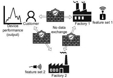
Figure 1: Problem scenario—forecasting device performance needs inputs from multiple parties, all of whom want to protect the confidentiality of their data.

Challenges. Despite its relevance, time-series forecasting with VFL has received limited attention [43]. This underscores the critical need for further exploration and research in this domain, especially considering three challenges that manufacturing scenarios introduce.

First, deep neural networks (DNNs) tend to overfit on manufacturing datasets since they can be affected by slow collection and noisy measurements, leading to small datasets [21, 11, 46]. Moreover, their complex parameter interactions limit their interpretability, which is needed for understanding the reasoning behind predictions to optimize production quality and downtime [41, 40].

Second, VFL is predominated by approaches utilizing a hierarchical split-learning architecture. This consists of several bottom models at the clients and a single top model held by a server [38, 16, 7]. The bottom models compute forward activations of their party’s sensitive features. The top model is held by a server that combines the intermediate activations to produce the output. Any party requiring forecasts would need the server to first produce the output, i.e., act as a middleman. This strong dependence on a single party is infeasible for several reasons. The server is a single point of failure which is catastrophic in case of data breaches. Moreover, it requires strong trust from the other parties as they are heavily reliant upon it for forecasting outputs. This is difficult to negotiate in manufacturing environments involving business competitors.

Third, while analytical/direct optimization methods like the normal equation [4] reach globally optimal solutions without requiring any hyperparameter tuning, they do not scale well to large problem instances, unlike iterative methods such as gradient descent. However, industries require both scalable and convenient solutions as they encounter diverse scenarios.

Contributions. To address these challenges, we develop a novel framework, Secret-Shared Time Series Forecasting with Vertical Federated Learning (STV), with the following contributions.

1. VFL forecasting framework. STV enables forecasting for VFL using Secret sharing (SS) [33] and secure multi-party computation (SMPC) [9, 24]. These do not involve privacy-performance trade-offs and offer cryptographic privacy guarantees. We propose STV_L for linear models such as SARIMAX [19, 29, 13], and STV_T for autoregressive trees (ARTs) [27].

2. Private, serverless inference. By adopting SS and SMPC, all computations and outputs are performed in a decentralized fashion by the parties involved. Thus, the outputs and intermediate data exist as distributed shares across all parties. STV ensures that the party requiring inference obtains the final predictions first-hand by collecting these shares. Due to the dispersion of shares, responsibility of output generation is distributed across all the involved parties, promoting trust through mutual dependence.

3. Adaptable optimization with Least Squares. STV_L uses a two-step approach with least squares (LS). This lends adaptability, as LS can be optimized using both iterative and direct methods. This requires protocols for $N$-party matrix multiplications and inverses on secretly shared data, a key novelty in our work. While iterative approaches like gradient descent scale better, direct optimization methods do not require hyperparameter tuning and guarantee global convergence. Therefore, we offer both options for tackling diverse forecasting scenarios.

We thoroughly evaluate STV on multiple fronts. First, we compare the forecasting accuracy of STV_L and STV_T with centralized state-of-the-art forecasters based on diffusion models [2], Long Short Term Memory (LSTM), and SARIMAX with Maximum Likelihood Estimation (MLE) [13]. Second, we compare the communication costs of iterative and direct optimization of linear forecasters under different scaling scenarios, highlighting their trade-offs. We use a wide range of datasets: five public datasets (Air quality, flight passengers, SML 2010, PV Power, Rossman Sales) and one real dataset from semiconductor manufacturing for measuring chip overlays from noisy alignment sensor data.

2 Background

In this section, we provide background knowledge on time series models and secure multiparty computation. We provide a summary of our notations and symbols in Table 1.

Table 1: Summary of key mathematical notations

Variable	Description
$X,Y$	Exogenous features and output variable
$H$	Time series polynomial
$.(t)$	Variable value at timestep $t$
$\epsilon$	Residual features
$\alpha,\beta,\gamma$	Autoregressive, moving average, exogenous coefficients
$\phi_{X},\phi_{Y}$	Time-lagged design matrix of features and output
$C_{1},C_{i\in[2:K]}$	Active party, passive parties
$\langle P\rangle$	Secret-shared state of a variable $P$. Union of $\langle P\rangle^{i}$
$\langle P\rangle^{i}$	$C_{i}$’s share of a variable $P$
$K$	Number of parties or clients

2.1 Time series forecasting

STV uses a popular linear forecaster, SARIMAX (Seasonal Auto-Regressive Integrated Moving Average with eXogenous variables) [19, 29], that generalizes other autoregresive forecasters [13, 28]. It models the series to forecast as a linear function composed of autoregressive, moving averages, and exogenous variables along with their seasonal counterparts [29].

Autoregressive terms capture the influence of earlier series outputs on future values. The moving average terms capture the influence of earlier errors/residuals. Finally, exogenous features serve as additional external features that may aid with forecasting. The seasonal counterparts model periodic patterns in the series. For example, output $Y$ at time $t$ can be represented using a polynomial $H$, containing residuals $\epsilon(t-i)$, past values $Y(t-i)$, and exogenous features $X_{j}(t)$ using a linear equation as follows:

The coefficients ($\alpha,\beta,\gamma$) can be estimated using least-squares (LS) [15, 26, 25, 37] or Maximum Likelihood Estimation (MLE) [13]. However, implementing MLE with multiparty computation and secret sharing is limited to likelihood functions like the exponential or multivariate normal distributions [35, 23], since computations with SMPC are limited to a small number of supported mathematical operations. However, least-squares optimization is still possible by extending basic SMPC protocols such as scalar addition and multiplication (see Section 2.2). First, the datasets, $(X,Y)$, are transformed into time-lagged design matrices, ($\phi_{X},\phi_{Y}$), to represent Equation 1:

In least-squares optimization, $A$ can be optimized using a two-step regression approach [37, 26, 15, 25]. First, the residuals are estimated by modeling using only autoregressive (AR) and exogenous terms. Then, all the coefficients in $A$ are jointly optimized by setting the residuals to the estimates.

Since the residuals, $\epsilon(.)$, in $\phi_{X}$ are unknown, they are initialized to zero to give $\hat{\phi_{X}}$, as shown below:

With mean-squared-error (MSE), $\hat{A}$ is optimized using the normal equation (NE) [4] or gradient descent (GD):

Gradient descent:

$$\hat{A}:=\hat{A}-\frac{\alpha}{N}\times(\hat{\phi_{X}})^{T}\times(\hat{\phi_{Y}}-\phi_{Y})\text{ (for $e$ iterations)}$$ (4)

Here, $\hat{\phi_{Y}}=\hat{\phi_{X}}\times\hat{A}$ are the predictions at a particular step, $\alpha$ is the learning rate and $N$ is the number of samples.

Normal equation:

$$\hat{A}=(({\hat{\phi_{X}}})^{T}\hat{\phi_{X})}^{-1}(({\hat{\phi_{X}}})^{T}{\phi_{Y}})`$$ (5)

Then, the residuals, $\varepsilon$, are then estimated as follows:

$$\varepsilon=\phi_{Y}-\hat{\phi_{X}}\times\hat{A}$$ (6)

These residual estimates are then re-substituted in Equation 2 to refine $A$ via a second optimization step.

While the above example is applicable to linear forecasters, the idea of autoregression can also be utilized for tree-based models like XGBoost [6]. This leads to the formulation of autoregressive trees (ARTs) [27], which use previous output values as decision nodes in a gradient-boosted regression tree. Therefore, extending VFL methods for XGBoost [42, 8, 10] to ARTs requires transforming the datasets into design matrices using a polynomial like Equation 1. While ARTs do not use residual terms, the tree-based architecture enables modeling forecasts in a non-linear fashion.

2.2 SMPC

Secure Multi-Party Computation methods use the principle of secret sharing [33] for privacy by scattering a value into random shares among parties. These methods offer strong privacy guarantees, i.e., information-theoretic security [10]. Assume there are $K$ parties, $C_{i\in[1,K]}$. If party $C_{i}$ wants to secure its private value, $V$, it does so by generating $K-1$ random shares, denoted $\langle V\rangle^{i^{\prime}}$ $\forall i^{\prime}\in[1,K];i^{\prime}\neq i$. These are sent to the corresponding party $C_{i^{\prime}}$. $C_{i}$’s own share is computed as $\langle V\rangle^{i}$ = $V$ - $\sum_{i^{\prime}\neq i}^{K}$$\langle V\rangle^{i^{\prime}}$. The whole ensemble of $K$ shares representing the shared state of $V$, is denoted as $\langle V\rangle$.

Parties cannot infer others’ data from their shares alone; however, the value can be recovered by combining all shares. By analogy, we distribute local features and outputs as shares to preserve their privacy. All parties then jointly utilize decentralized training protocols on the secretly shared data to obtain a local model. Inference/forecasting is done by distributing features into secret shares and then computing the prediction as a distributed share across all parties.

Training and forecasting on secretly shared features requires primitives for performing mathematical operations on distributed shares, which we explain as follows.

Addition and subtraction: If $X$ and $Y$ exist as secret shares, $\langle X\rangle$ and $\langle Y\rangle$, each party performs a local addition or subtraction, i.e., $\langle Z\rangle^{k}$ = $\langle X\rangle^{k}$ $+(-)$ $\langle Y\rangle^{k}$. To obtain $Z=X+(-)Y$, the shares are aggregated: $Z=\sum_{k}^{K}$$\langle Z\rangle^{k}$.

Knowing the value of $\langle Z\rangle^{k}$ makes it impossible to infer the private values $X$ or $Y$, as each participant only owns a share of the whole secret. Moreover, the individual values of the shares, $\langle X\rangle^{k}$ and $\langle Y\rangle^{k}$, are also masked by adding them.

Multiplication (using Beaver’s triples) [3, 42]: Consider $Z=X*Y$, where $*$ denotes element-wise multiplication, and $X$ and $Y$, are secretly shared. The coordinator first generates three numbers $a,b,c$ such that $c=a*b$. These are then secretly shared, i.e., $C_{k}$, receives $\langle a\rangle^{k}$, $\langle b\rangle^{k}$, and $\langle c\rangle^{k}$. $C_{k}$ computes $\langle e\rangle^{k}$ = $\langle X\rangle^{k}$ - $\langle a\rangle^{k}$ and $\langle f\rangle^{k}$ = $\langle Y\rangle^{k}$ - $\langle b\rangle^{k}$, and sends it to $C_{1}$. $C_{1}$ then aggregates these shares to recover $e$ and $f$ and broadcasts them to all parties. $C_{1}$ then computes $\langle Z\rangle^{1}$ = $e*f$+$f*$$\langle a\rangle^{1}$+ $e*$$\langle b\rangle^{1}$+$\langle c\rangle^{1}$, and the others calculate $\langle Z\rangle^{k}$ = $f*$$\langle a\rangle^{k}$+$e*$$\langle b\rangle^{k}$+$\langle c\rangle^{k}$. It is easy to see that aggregation of the individual shares gives the product $Z$.

Despite knowing $e$ and $f$, $X$ and $Y$ are hidden since the parties do not know $a,b,$ and $c$. Similar to addition, the individual shares, $\langle Z\rangle^{k}$, do not reveal anything about the local share values, i.e., $\langle X\rangle^{k}$, $\langle Y\rangle^{k}$, $\langle a\rangle^{k}$, $\langle b\rangle^{k}$, and $\langle c\rangle^{k}$.

Additional primitives such as division, argmax, and sigmoid can also be computed using secret sharing, the details of which are provided in Fang et al. [10] and Xie et al. [42].

3 STV Framework

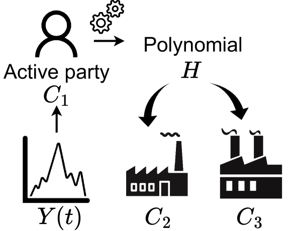
(a) Polynomial generation through pre-preocessing

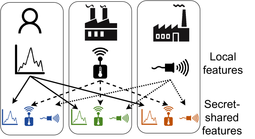
(b) Secretly sharing features

Figure 2: Time-series pre-processing and secret sharing of features in STV

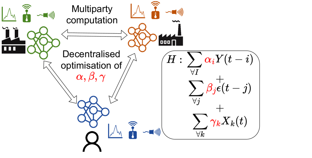
(a) MPC optimization of time-series polynomial $H$ with secret-shared features

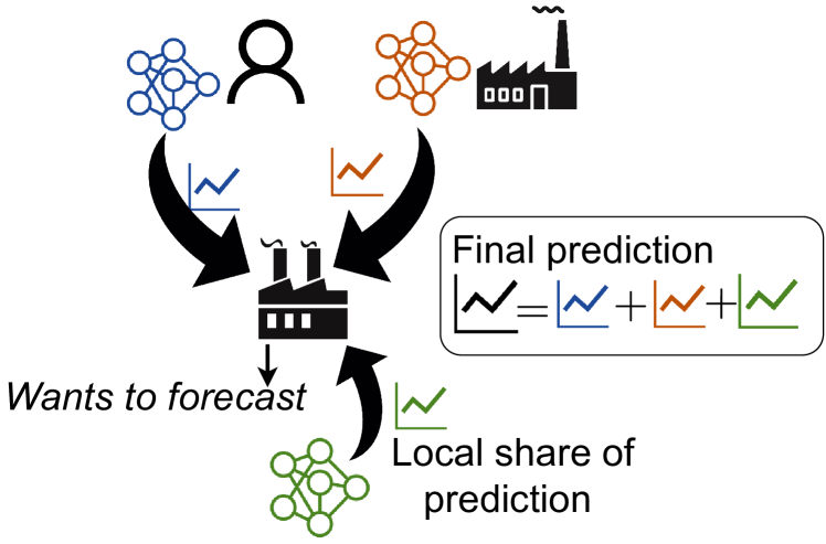
(b) Decentralized inference through flexible selection of share-aggregator

Figure 3: Decentralized training and inference in STV

Algorithm 1 General protocol STV

Data: $X_{k}$ on party $C_{k}$ $\forall k\in[1,K]$, and $Y$ on $C_{1}$

Accepted Parameters: Task: Training/Inference, Model type, number of trees $T$, Optimization method $O$, learning rate $\alpha$, iterations, $e$, Trained distributed $Model$, Requesting party $C_{j}$

Output:Trained model distributed across $K$ parties or final inference result on party $C_{j}$

1:  if $Training$ and active party $C_{1}$ then

2:      params = ProcessSeries(Y)

3:     H = GenPoly (params, type)

4:     Broadcast $H$ to $C_{i}$ $\forall i\in[1,K]$

5:  end if

6:  Share local features $\langle X_{k}\rangle$ and (or) outputs $\langle Y\rangle$

7:  $\langle\phi_{X}\rangle$,$\langle\phi_{Y}\rangle$ = TransformData ($H$){ Equation 2}

8:  if type == Tree and Training then

9:     return  $Model$ = STV_T ($\langle\phi_{X}\rangle$, $\langle Y\rangle$,T)

10:  else if type == Linear and Training then

11:     return  $Model$ = STV_L ($\langle\phi_{X}\rangle$,$\langle\phi_{Y}\rangle$, O, $\alpha$, $e$)

12:  end if

13:  if Inference then

14:     $\langle Result\rangle$ = $Model.Predict$($\langle\phi_{X}\rangle$)

15:     if requesting party $C_{j}$ then

16:        $Result$ = $\sum_{k=1}^{K}$$\langle Result\rangle^{k}$ {Aggregate predictions}

17:     end if

18:  end if

Algorithm 2 STV_T

Data: Secretly shared transformed matrices $\langle\phi_{X}\rangle$, $\langle\phi_{Y}\rangle$

Parameter: number of trees $T$

Output: Distributed autoregressive XGBoost tree

1:  Initialize predictions $\langle\hat{\phi_{Y}}\rangle^{k}$$=0$ on all parties $C_{k}$

2:  Initialize $Trees_{k}$ = [ ] on all parties $C_{k}$

3:  for $t\in[1,T]$ do

4:     $tree_{t_{k}}$ = SecureFit($\langle\phi_{X}\rangle^{k}$,$\langle\phi_{Y}\rangle^{k}$,$\langle\hat{\phi_{Y}}\rangle^{k}$)

5:     $\langle\hat{\phi_{Y_{t}}}\rangle^{k}$ = $tree_{t_{k}}.$Predict($\langle\phi_{X}\rangle^{k}$)

6:     if active party $C_{1}$ then

7:        $\hat{\phi_{Y_{t}}}=\sum_{i=1}^{K}$$\langle\hat{\phi_{Y_{t}}}\rangle^{k}${Aggregate predictions}

8:        $\hat{\phi_{Y}}=\hat{\phi_{Y}}+\hat{\phi_{Y_{t}}}${Add to final predictions}

9:     end if

10:     $Trees_{k}.append(tree_{t_{k}})$ on every party $C_{k}$

11:  end for

12:  return  $Trees_{k}$ on party $C_{k}$

Algorithm 3 STV_L

Data: Secretly shared transformed matrices $\langle\phi_{X}\rangle$, $\langle\phi_{Y}\rangle$

Accepted Parameters: $O$, $\alpha$, $e$

Output: Shared optimized coefficients $\langle A\rangle$

1:  for $step\in[1,2]$ do

2:     if $step=1$ then

3:        Initialize residuals to zero in $\langle\phi_{X}\rangle^{k}$ for all $C_{k}$

4:     end if

5:     if $O=``iterative"$ then

6:        Randomly initialize $\langle A\rangle^{k}$ for all $C_{k}$

7:        for $e$ iterations do

8:           Get $\langle\hat{\phi_{Y}}\rangle$ = $\langle\phi_{X}\rangle$$\times$$\langle A\rangle$ using Alg. 4

9:           $\langle\odv{l}{A}\rangle$ = ($\langle{\phi_{X}}\rangle$)^T$\times$$($$\langle\hat{\phi_{Y}}\rangle$ - $\langle\phi_{Y}\rangle$$)$ (Alg. 4)

10:           Perform update: $\langle A\rangle$ := $\langle A\rangle$ - $\frac{\alpha}{N}$$\langle\odv{l}{A}\rangle$

11:        end for

12:     else if $O=``direct"$ then

13:        $\langle Z\rangle$ = ($\langle\phi_{X}\rangle$)${}^{T}\times$$\langle\phi_{X}\rangle$ using Alg. 4

14:        $\langle W\rangle$ = $\langle Z^{-1}\rangle$ using Alg. 5

15:        $\langle V\rangle$ = ($\langle\phi_{X}\rangle$)${}^{T}\times$$\langle\phi_{Y}\rangle$ using Alg. 4

16:        $\langle A\rangle$ = $\langle W\rangle$ $\times$ $\langle V\rangle$

17:     end if

18:     if $step=1$ then

19:        Predict: $\langle\hat{\phi_{Y}}\rangle$ = $\langle\phi_{X}\rangle$ $\times$ $\langle A\rangle$ using Alg. 4

20:        Estimate residuals $\langle\varepsilon\rangle$ = $\langle\phi_{Y}\rangle$ - $\langle\hat{\phi_{Y}}\rangle$

21:        Set $\langle\phi_{X}\rangle^{k}$ using residuals from $\langle\varepsilon\rangle^{k}$ for all $C_{k}$

22:     end if

23:  end for

24:  return  $\langle A\rangle^{k}$ on all parties $C_{k}$

Algorithm 4 Secure Matrix Multiplication

Data: Secretly shared matrices $\langle U\rangle$ and $\langle V\rangle$ across $K$ parties, $C_{1},C_{2},..,C_{K}$

Output: $\langle W\rangle$, i.e., product $W=U\times V$ as shares across $K$ parties

1:  for each row index $i$ do

2:     for each column index $j$ do

3:        $\langle\vec{T}\rangle$ = $\langle\vec{U[i,:]}\rangle$ * $\langle\vec{V[:,j]}\rangle$ {Element-wise product} $\langle W_{i,j}\rangle^{k}$ = $sum\{$$\langle\vec{T}\rangle^{k}$$\}$

4:     end for

5:  end for

6:  return  $\langle W\rangle^{k}$ on party $C_{k}$

Algorithm 5 Secure Matrix Inverse

Data: Secretly shared matrix $\langle U\rangle$ across $K$ parties, $C_{1},C_{2},..,C_{K}$

Output: $\langle V\rangle$, i.e., inverse, $V=U^{-1}$, as a distributed share

1:  if active party ($P_{1}$) then

2:     Generate random non-singular perturbation matrix $P$ and secretly share as $\langle P\rangle$

3:  end if

4:  Get $\langle Q\rangle$ = $\langle U\rangle$ $\times$ $\langle P\rangle$ using Alg. 4

5:  Aggregate $Q$ = $\sum_{k=1}^{K}$$\langle Q\rangle^{k}$ on passive party $C_{j};j>1$

6:  if Passive party $C_{j}$ then

7:     Compute $R=Q^{-1}=(UP)^{-1}=P^{-1}U^{-1}$

8:     Generate shares $\langle R\rangle$

9:  end if

10:  Compute $\langle T\rangle$ = $\langle U^{-1}\rangle$ = $\langle P\rangle$ $\times$ $\langle R\rangle$ using Alg. 4

11:  return  $\langle T\rangle^{k}$ on party $C_{k}$

Here we introduce the adversarial model and problem statement, followed by STV’s design and implementation for ART, STV_T, and SARIMAX forecasters, STV_L. For both models, secret sharing and SMPC are used to protect the privacy of input features.

Adversarial Models. We assume that all parties are honest-but-curious/semi-honest [16, 44], i.e., they adhere to protocol but try to infer others’ private data using their own local data and whatever is communicated to them. Also, it is assumed that parties do not collude. This is a standard assumption in VFL as all parties are incentivised to collaborate due to their mutual dependence on one another for training and inference [44, 16]. In addition, we also assume that communication between parties is encrypted.

Problem Statement. We assume a setup with $K$ parties, $C_{1}$ to $C_{K}$, grouped into two types: $active$ and $passive$. The active party, $C_{1}$, owns the outputs of the training data for the time series, $Y(t)$, for timestep $t$. It also possesses exogenous features, $X_{1}(t)$. The passive parties only have exogenous features, $X_{i},\forall i\in[2,K]$. The common samples between parties are assumed to be already identified using privacy-preserving entity alignment approaches [16, 32]. Our goal is to forecast future values using exogenous and autoregressive features without sharing them with others in plaintext.

We further assume that there is a coordinator, a trusted third party that oversees the training process and is responsible for generating randomness, such as Beaver’s triples for element-wise multiplication with SMPC [3, 10]. The coordinator cannot access private data and intermediate results, so it does not pose a privacy threat, as mentioned by Xie et al. [42].

3.1 Protocol Overview

An overview of STV is provided in Algorithm 1. The framework consists of preliminary steps for pre-processing the series and secretly sharing the input features (Figure 2), followed by decentralized training and inference (Figure 3).

Training. To start, the active party initiates by pre-processing the output and determines parameters like the auto-correlations and partial auto-correlations of the series (line 2). As illustrated in 2(a), these are then used to generate a polynomial for SARIMAX or ARTs (line 3). As illustrated in 2(b), the features and outputs are then secretly shared and transformed into lagged design matrices (line 7), like in Equation 2. All parties then follow decentralized training protocols, Algorithm 2 or Algorithm 3 to train a distributed model. Training is illustrated in 3(a).

Privacy-preserving inference. During inference (3(b)), the final prediction exists as a distributed share (line 14), which is aggregated on the requesting party (line 16). Since the result is computed as a distributed share, the outputs are not produced by a sole party, which makes the inference serverless.

3.2 STV_T: Autoregressive tree (ART)

STV_T focuses on the autoregressive tree and the first step is to transform the original datasets, $X$ and $Y$, into time-lagged design matrices. Following the training framework in Xie et al. [42], we train a distributed autoregressive XGBoost model using the secretly-shared design matrices. The details are provided in Algorithm 2.

Training proceeds iteratively, finally resulting in the generation of $T$ trees on each party. At each step, every party learns a new tree and makes a local prediction (lines 4-5). The active participant aggregates the distributed shares of the prediction to compute the first and second order gradients needed for generating the next distributed tree. These gradients are then secretly shared with the other parties for them update their local tree ensembles. Details on the tree-building function, SecureFit, are provided in Appendix C.

During training, individual predictions are aggregated on the active party since gradients are computed by $C_{1}$ (see Appendix C). For inference, aggregation can be performed on any party since gradients are not calculated. This enables serverless forecasting.

3.3 STV_L: SARIMAX

With STV_L, the objective is optimizing the coefficients, $A$, in Equation 2. This can be done either directly or iteratively using the two-step regression process explained in Section 2.1. Details are provided in Algorithm 3.

Several steps in Algorithm 3 require matrix operations like multiplications (lines 8-9; 13-19) and inverse (line 14) on secretly shared data. This is a requirement for both iterative and direct methods, as seen in Equation 5 and Equation 4. We design novel $N$-party ($\geq 2$) algorithms for performing these operations, as detailed below.

N-party matrix multiplication. To perform matrix multiplication with secretly shared data (algorithm 4), we view the computation of every output element $W_{i,j}$ as a scalar product of row and column vectors (line 3). This can be implemented using the $N$-party element-wise product of the row and column vectors with Beaver’s triples followed by an addition operation, as shown in Section 2.2.

N-party matrix inverse. For matrix inverses (Algorithm 5), we compute the inverse of a secretly-shared matrix, $U$, using a non-singular perturbation matrix, $P$, generated by the active party (line 2). Subsequently, the aggregation of product $UP$ on a passive party does not leak $U$ as the party does not know $P$ (line 5). $(UP)^{-1}$ can then be computed locally and secretly shared, followed by a matrix multiplication with $P$, i.e., $P\times(UP)^{-1}=U^{-1}$, giving the result as a secret share (lines 7-10).

Similar to the tree-based models, forecasting is done by secretly sharing features and computing the output as a distributed share (see 3(b)). The true value of the forecast can be obtained by summing the shares across all parties, enabling serverless inference.

4 Experiments

We evaluate the forecasting accuracy of STV against centralized approaches. We also compare the scalability of iterative and direct optimization for linear forecasters using the total communication cost.

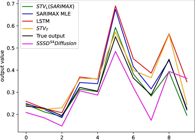
(a) Airquality (50)

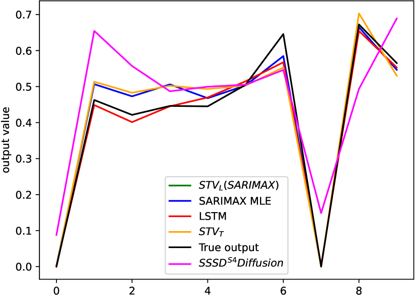
(b) Rossman Sales (50)

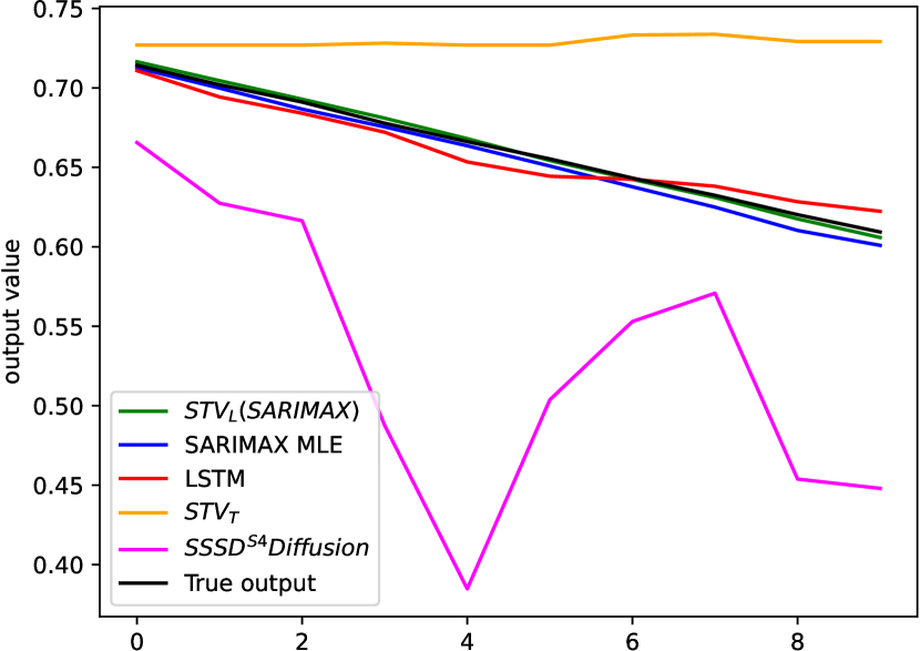
(c) SML 2010 (50)

Figure 4: Forecasts from one of the windows of total size 50 (40 train, 10 test) from three datasets.

Table 2: Average $n$-MSE and (standard deviation) results for different datasets and methods. Relative improvement of the best VFL method with the best centralized one is also shown (rel. imp). Lowest MSE values are highlighted in bold. SML 2010, Air quality, and Rossman Sales have prequential window sizes 50, 100, 200, and 400. PV Power uses 25, 50, 100, and 200. Airline passengers uses 60, 80, 100, 120, and 140. Finally, the industrial data uses 25, 50, and 100.

Dataset	STVL	STVT	SARIMAX	LSTM	SSSDS4	Rel. imp. (%)
	(SARIMAX, VFL)	(ART, VFL)	(MLE, Centralized)	(Centralized)	(Centralized)
Airquality	0.00069	0.00100	0.00088	0.00114	0.00150	21.59
	(0.00008)	(0.00056)	(0.00031)	(0.00076)	(0.00073)
Airline passengers	0.00304	0.00808	0.00222	0.04130	0.00392	-36.94
	(0.00086)	(0.00379)	(0.00148)	(0.04086 )	(0.00226)
PV Power	0.00138	0.00249	0.00159	0.14333	0.00167	15.22
	(0.00136)	(0.00254)	(0.00095)	(0.23033)	(0.00058)
SML 2010	0.00787	0.01875	0.01033	0.01716	0.01085	23.81
	(0.00711)	(0.01458)	(0.01061)	(0.01086)	(0.00871)
Rossman Sales	0.00074	0.00243	0.00077	0.00639	0.00331	3.89
	(0.00012)	(0.00153)	(0.00006)	(0.00280)	(0.00151)
Industrial data	0.00602	0.04118	0.00969	0.00617	0.01875	2.43
	(0.00049)	(0.04051)	(0.00449)	(0.00203)	(0.00313)

4.1 Forecasting accuracy

We compare the performance of STV_L (direct optimization) and STV_T with other centralized methods: Long-Short-Term Memory (LSTM), SARIMAX with MLE, and diffusion models for forecasting (SSSD^S4) [2].

The LSTM has two layers of 64 LSTM units each, followed by two dense layers of size 32 and 1. We train the model for 500 epochs and use a batch size of 32 with a default learning rate of 0.001. The diffusion configuration has the following settings: $T=200,\beta_{0}=0.0001,\beta_{T}=0.02$. For the diffusion model, we use two residual layers, four residual and skip channels, with three diffusion embedding layers of dimensions $8\times 16$. Training is done for 4000 iterations with a learning rate of 0.002.

Five public forecasting datasets are used: Airline passengers [20], Air quality data [39], PV Power [17], SML 2010 [30], and Rossman Sales [1]. An industry-specific dataset to estimate a performance parameter for chip overlays from inline sensor values in semiconductor manufacturing is also included [11, 12]. Additional details on the datasets, evaluation, and pre-processing are given in Appendix A and Appendix B.

A variant of prequential window testing [5] is used since industrial time series data can significantly change after intervals due to machine changes/repairs. The dataset is partitioned into multiple windows of a given size, each further divided into an 80-20 train-test split. After forecasting the test split, the model is retrained on the next window (refer Appendix B).

All features and outputs are scaled between 0 and 1 for a consistent comparison. We thus present the predictions’ normalized mean-squared errors ($n$-MSE). Ground truths on the test set are measured and averaged across multiple windows. We average the $n$-MSE scores across different window sizes to generalize performance scores across varying forecasting ranges, as shown in Table 2.

Table 2 demonstrates that our approach STV_L outperforms other centralized methods in terms of performance. We use direct optimization since iterative gradient descent eventually converges to the same value in the long run. Due to its guaranteed convergence, direct optimization improves against centralized methods by up to 23.81%. Though it does worse than SARIMAX MLE on the passenger data, it is still among the top two methods.

We also show three regression plots from a prequential window of size 50 from three datasets in Figure 4. In general, all the methods can capture patterns in the time series, like in 4(a) and 4(b). However, deep models such as SSSD^S4 occasionally overfit, showing the drawback of NNs on small windows (see 4(c)).

4.2 Scalability

We measure the total communication costs of direct optimization using the normal equation (NE) and iterative batch gradient descent (GD) to analyze the scalability of the two methods under increasing parties, features, and samples.

We vary the parties between 2, 4, and 8, features between 10 and 100, and samples between 10, 100, and 1000. Since communication costs depend only on the dataset dimensions and the number of parties, we generate random data matrices for all valid combinations of features and samples on each party, i.e., #features $\leq$ #samples. We then optimize the coefficients using either the direct approach (Algorithm 3, lines (13-19)), or batch gradient descent (lines (6-10)), for a different number of iterations (10, 100, 1000). For party-scaling, we average the total communication costs across various feature and sample combinations for a given number of parties. Similarly, we measure feature and sample scaling by averaging the total costs across different (sample, party) and (feature, party) combinations. Results are shown in Table 3, Table 4, and Table 5.

Table 3: Average total communication sizes (bytes) under varying party count.

parties	NE	GD iterations
		10	100	1000
2	2.54$\times 10^{8}$	2.33$\times 10^{7}$	2.33$\times 10^{8}$	2.33$\times 10^{9}$
4	5.85$\times 10^{8}$	4.65$\times 10^{7}$	4.65$\times 10^{8}$	4.65$\times 10^{9}$
8	1.48$\times 10^{9}$	9.31$\times 10^{7}$	9.31$\times 10^{8}$	9.31$\times 10^{9}$

Table 4: Average total communication sizes (bytes) with varying feature counts.

Features	NE	GD iterations
		10	100	1000
10	9.77$\times 10^{6}$	8.34$\times 10^{6}$	8.34$\times 10^{7}$	8.34$\times 10^{8}$
100	1.92$\times 10^{9}$	1.23$\times 10^{8}$	1.23$\times 10^{9}$	1.23$\times 10^{10}$

Table 5: Average of total communication sizes (bytes) with varying samples.

Samples	NE	GD iterations
		10	100	1000
10	1.16$\times 10^{6}$	2.76$\times 10^{5}$	2.76$\times 10^{6}$	2.76$\times 10^{7}$
100	4.53$\times 10^{8}$	1.24$\times 10^{7}$	1.24$\times 10^{8}$	1.24$\times 10^{9}$
1000	1.48$\times 10^{9}$	1.23$\times 10^{8}$	1.23$\times 10^{9}$	1.23$\times 10^{10}$

Our observation from these three tables is that when the number of parties/samples/features is small, direct optimization’s cost is comparable to an iterative version with more iterations. For example, when the number of parties is 2, we see that the cost of NE is close to GD with 100 iterations in Table 3. However, when we increase to 8 parties, the cost of NE exceeds GD with 100 iterations.

Similarly, in Table 4 and Table 5, we see that NE has a lower cost than GD with 100 iterations for smaller magnitudes of features and samples. This is no longer the case when increasing the features and samples.

However, the cost of GD increases proportionally with the iterations, and at some point, it becomes more expensive than NE, as we see with 1000 iterations. In practice, hyperparameters like the learning rate affect the steps required for convergence, which may be hard to tune in a distributed setup. So, choosing between iterative or direct optimization depends on several factors, requiring adaptability in frameworks.

5 Related Work

We direct our attention to the selected works presented in Table 6 to represent closely related research in VFL comprehensively. We compare the methods’ applicability to time series forecasting, whether inference privacy can be easily achieved through decentralization, their adaptability to alternative optimization choices, and whether they can generalize to $N$-parties.

Time-series forecasting. Earlier, we mentioned that industries require easy-to-understand and low-complexity models to avoid overfitting on small datasets. In this light, we focus on linear/logistic regression (LR) [16, 14, 34], and tree-based models [42, 8], with transparent structures that are considered inherently interpretable [31, 45]. Yan et al. [43] modifies the split learning architecture using Gated Recurrent Units (GRUs) with a shared upper model for predictions. However, its dependence on a single server for generating predictions is a bottleneck and can lead to trust issues among the involved parties. Nevertheless, to the best of our knowledge, this remains the only other method for time-series forecasting with VFL.

Serverless inference. We consider schemes adopting SS as potential candidates for serverless inference requirements, as these can be seamlessly integrated with a decentralized approach akin to ours [42, 34, 14]. Shi et al. [34] and Han et al. [14] train linear models while Xie et al. [42] implement XGBoost. Homomorphic encryption methods, such as Hardy et al. [16], require the predictions to be decrypted at the server, violating the requirement.

Optimization. When it comes to optimization techniques, all selected works, except for Han et al. [14], employ solely iterative approaches. Notably, Han et al. [14] offer iterative and matrix-based methods for direct optimization using Equation 5. This requires computing matrix multiplications and inverses, only implemented for the two-party case. To the best of our knowledge, ours is the first $N$-party protocol for performing these operations.

Table 6: Comparison of related works in VFL.

Method	Time Series	Serverless inference	Dual optimization	N-party ($\geq 2$)
Yan et al. [43]	✔	✖	✖	✔
Han et al.[14]	✖	✔	✔	✖
Xie et al.[42]	✖	✔	✖	✔
Shi et al.[34]	✖	✔	✖	✔
STV (ours)	✔	✔	✔	✔

6 Applications

In this work, Additionally, the challenge of slow data collection is also prevalent in domains as often real datasets need to be collected via manually conducting surveys or interviews.

7 Conclusion and Discussion

This work presents a novel decentralized and privacy-preserving forecasting framework. Here, we focus on the manufacturing industry as a motivating example for our problem scenario. However, our framework’s applicability also extends to other domains, such as healthcare and finance, which face similar constraints. For example, collaborating healthcare centers can jointly benefit from sharing patient features to model patient risk levels. However, patient confidentiality agreements may pose restrictions to sharing data.

Our results show that our approach is competitive against centralized methods. Scalability analyses show the nuanced dynamics between iterative and direct optimization, highlighting the need for an adaptable framework.

For the future, several paths of exploration beckon. First, the models used in this study are weaker at capturing long-range patterns in time series data, for which LSTMs and diffusion models are better suited. We aim to enable these models for VFL. Second, current VFL cases assume a static set of participants. Exploring a hybrid of horizontal FL and VFL elements would be interesting if VFL model clusters were independently trained and aggregated to enhance their collective forecasting power. Going beyond semi-honest participants to malicious adversaries is another possibility.

References

- ros [2015] Rossman store sales, 2015. URL https://www.kaggle.com/c/rossmann-store-sales.
- Alcaraz and Strodthoff [2022] J. M. L. Alcaraz and N. Strodthoff. Diffusion-based time series imputation and forecasting with structured state space models. arXiv preprint arXiv:2208.09399, 2022.
- Beaver [1992] D. Beaver. Efficient multiparty protocols using circuit randomization. In Advances in Cryptology—CRYPTO’91: Proceedings 11, pages 420–432. Springer, 1992.
- Blais et al. [2010] J. Blais et al. Least squares for practitioners. Mathematical Problems in Engineering, 2010, 2010.
- Cerqueira et al. [2020] V. Cerqueira, L. Torgo, and I. Mozetič. Evaluating time series forecasting models: An empirical study on performance estimation methods. Machine Learning, 109:1997–2028, 2020.
- Chen et al. [2015] T. Chen, T. He, M. Benesty, V. Khotilovich, Y. Tang, H. Cho, K. Chen, R. Mitchell, I. Cano, T. Zhou, et al. Xgboost: extreme gradient boosting. R package version 0.4-2, 1(4):1–4, 2015.
- Chen et al. [2020] T. Chen, X. Jin, Y. Sun, and W. Yin. Vafl: a method of vertical asynchronous federated learning. arXiv preprint arXiv:2007.06081, 2020.
- Cheng et al. [2021] K. Cheng, T. Fan, Y. Jin, Y. Liu, T. Chen, D. Papadopoulos, and Q. Yang. Secureboost: A lossless federated learning framework. IEEE Intelligent Systems, 36(6):87–98, 2021.
- Cramer et al. [2015] R. Cramer, I. B. Damgård, et al. Secure multiparty computation. Cambridge University Press, 2015.
- Fang et al. [2021] W. Fang, D. Zhao, J. Tan, C. Chen, C. Yu, L. Wang, L. Wang, J. Zhou, and B. Zhang. Large-scale secure xgb for vertical federated learning. In Proceedings of the 30th ACM International Conference on Information & Knowledge Management, pages 443–452, 2021.
- Gkorou et al. [2017] D. Gkorou, A. Ypma, G. Tsirogiannis, M. Giollo, D. Sonntag, G. Vinken, R. van Haren, R. J. van Wijk, J. Nije, and T. Hoogenboom. Towards big data visualization for monitoring and diagnostics of high volume semiconductor manufacturing. In Proceedings of the Computing Frontiers Conference, CF’17, page 338–342, New York, NY, USA, 2017. Association for Computing Machinery. ISBN 9781450344876. 10.1145/3075564.3078883. URL https://doi.org/10.1145/3075564.3078883.
- Gkorou et al. [2020] D. Gkorou, M. Larranaga, A. Ypma, F. Hasibi, and R. J. van Wijk. Get a human-in-the-loop: Feature engineering via interactive visualizations. 2020.
- Hamilton [2020] J. D. Hamilton. Time series analysis. Princeton university press, 2020.
- Han et al. [2009] S. Han, W. K. Ng, L. Wan, and V. C. Lee. Privacy-preserving gradient-descent methods. IEEE transactions on knowledge and data engineering, 22(6):884–899, 2009.
- Hannan and Kavalieris [1984] E. J. Hannan and L. Kavalieris. A method for autoregressive-moving average estimation. Biometrika, 71(2):273–280, 1984.
- Hardy et al. [2017] S. Hardy, W. Henecka, H. Ivey-Law, R. Nock, G. Patrini, G. Smith, and B. Thorne. Private federated learning on vertically partitioned data via entity resolution and additively homomorphic encryption. arXiv preprint arXiv:1711.10677, 2017.
- Kannal [2020] A. Kannal. Solar power generation, 2020. URL https://www.kaggle.com/datasets/anikannal/solar-power-generation-data.
- Konečnỳ et al. [2015] J. Konečnỳ, B. McMahan, and D. Ramage. Federated optimization: Distributed optimization beyond the datacenter. arXiv preprint arXiv:1511.03575, 2015.
- Korstanje [2021] J. Korstanje. The SARIMAX Model, pages 125–131. Apress, Berkeley, CA, 2021. ISBN 978-1-4842-7150-6. 10.1007/978-1-4842-7150-6_8. URL https://doi.org/10.1007/978-1-4842-7150-6_8.
- Kothari [2018] C. Kothari. Airline passengers, 2018. URL https://www.kaggle.com/datasets/chirag19/air-passengers.
- Li et al. [2021] L. Li, S. K. Damarla, Y. Wang, and B. Huang. A gaussian mixture model based virtual sample generation approach for small datasets in industrial processes. Information Sciences, 581:262–277, 2021.
- Lin et al. [2019] C.-Y. Lin, Y.-M. Hsieh, F.-T. Cheng, H.-C. Huang, and M. Adnan. Time series prediction algorithm for intelligent predictive maintenance. IEEE Robotics and Automation Letters, 4(3):2807–2814, 2019.
- Lin and Karr [2010] X. Lin and A. F. Karr. Privacy-preserving maximum likelihood estimation for distributed data. Journal of Privacy and Confidentiality, 1(2), 2010.
- Lindell [2005] Y. Lindell. Secure multiparty computation for privacy preserving data mining. In Encyclopedia of Data Warehousing and Mining, pages 1005–1009. IGI global, 2005.
- Liu et al. [2016] C. Liu, S. C. Hoi, P. Zhao, and J. Sun. Online arima algorithms for time series prediction. In Proceedings of the AAAI conference on artificial intelligence, volume 30, 2016.
- Lütkepohl [2007] H. Lütkepohl. General-to-specific or specific-to-general modelling? an opinion on current econometric terminology. Journal of Econometrics, 136(1):319–324, 2007.
- Meek et al. [2002] C. Meek, D. M. Chickering, and D. Heckerman. Autoregressive tree models for time-series analysis. In Proceedings of the 2002 SIAM International Conference on Data Mining, pages 229–244. SIAM, 2002.
- Montgomery et al. [2015] D. C. Montgomery, C. L. Jennings, and M. Kulahci. Introduction to time series analysis and forecasting. John Wiley & Sons, 2015.
- Perktold [2023] J. Perktold. Sarimax, 2023. URL https://www.statsmodels.org/dev/generated/statsmodels.tsa.statespace.sarimax.SARIMAX.html.
- Romeu-Guallart and Zamora-Martinez [2014] P. Romeu-Guallart and F. Zamora-Martinez. SML2010. UCI Machine Learning Repository, 2014. DOI: https://doi.org/10.24432/C5RS3S.
- Samek and Müller [2019] W. Samek and K.-R. Müller. Towards explainable artificial intelligence. Explainable AI: interpreting, explaining and visualizing deep learning, pages 5–22, 2019.
- Scannapieco et al. [2007] M. Scannapieco, I. Figotin, E. Bertino, and A. K. Elmagarmid. Privacy preserving schema and data matching. In Proceedings of the 2007 ACM SIGMOD international conference on Management of data, pages 653–664, 2007.
- Shamir [1979] A. Shamir. How to share a secret communications of the acm, 22, 1979.
- Shi et al. [2022] H. Shi, Y. Jiang, H. Yu, Y. Xu, and L. Cui. Mvfls: multi-participant vertical federated learning based on secret sharing. The Federate Learning, pages 1–9, 2022.
- Snoke et al. [2017] J. Snoke, T. R. Brick, A. Slavkovic, and M. D. Hunter. Providing accurate models across private partitioned data: Secure maximum likelihood estimation, 2017.
- Susto and Beghi [2016] G. A. Susto and A. Beghi. Dealing with time-series data in predictive maintenance problems. In 2016 IEEE 21st International Conference on Emerging Technologies and Factory Automation (ETFA), pages 1–4. IEEE, 2016.
- Tarsitano and Amerise [2017] A. Tarsitano and I. L. Amerise. Short-term load forecasting using a two-stage sarimax model. Energy, 133:108–114, 2017.
- Vepakomma et al. [2018] P. Vepakomma, O. Gupta, T. Swedish, and R. Raskar. Split learning for health: Distributed deep learning without sharing raw patient data. arXiv preprint arXiv:1812.00564, 2018.
- Vito [2016] S. Vito. Air Quality. UCI Machine Learning Repository, 2016. DOI: https://doi.org/10.24432/C59K5F.
- Vollert et al. [2021] S. Vollert, M. Atzmueller, and A. Theissler. Interpretable machine learning: A brief survey from the predictive maintenance perspective. In 2021 26th IEEE International Conference on Emerging Technologies and Factory Automation (ETFA ), pages 01–08, 2021. 10.1109/ETFA45728.2021.9613467.
- Wang et al. [2022] J. Wang, Y. Li, R. X. Gao, and F. Zhang. Hybrid physics-based and data-driven models for smart manufacturing: Modelling, simulation, and explainability. Journal of Manufacturing Systems, 63:381–391, 2022.
- Xie et al. [2022] L. Xie, J. Liu, S. Lu, T.-H. Chang, and Q. Shi. An efficient learning framework for federated xgboost using secret sharing and distributed optimization. ACM Transactions on Intelligent Systems and Technology (TIST), 13(5):1–28, 2022.
- Yan et al. [2022] Y. Yan, G. Yang, Y. Gao, C. Zang, J. Chen, and Q. Wang. Multi-participant vertical federated learning based time series prediction. In Proceedings of the 8th International Conference on Computing and Artificial Intelligence, pages 165–171, 2022.
- Yang et al. [2019] Q. Yang, Y. Liu, T. Chen, and Y. Tong. Federated machine learning: Concept and applications. ACM Transactions on Intelligent Systems and Technology (TIST), 10(2):1–19, 2019.
- Zhang et al. [2021] Y. Zhang, P. Tiňo, A. Leonardis, and K. Tang. A survey on neural network interpretability. IEEE Transactions on Emerging Topics in Computational Intelligence, 5(5):726–742, 2021. 10.1109/TETCI.2021.3100641.
- Zhu et al. [2023] Q.-X. Zhu, H.-T. Zhang, Y. Tian, N. Zhang, Y. Xu, and Y.-L. He. Co-training based virtual sample generation for solving the small sample size problem in process industry. ISA transactions, 134:290–301, 2023.