Information Theoretic Text-to-Image Alignment

Abstract

Diffusion models for Text-to-Image (t2i) conditional generation have seen tremendous success recently. Despite their success, accurately capturing user intentions with these models still requires a laborious trial and error process. This challenge is commonly identified as a model alignment problem, an issue that has attracted considerable attention by the research community. Instead of relying on fine-grained linguistic analyses of prompts, human annotation, or auxiliary vision-language models to steer image generation, in this work we present a novel method that relies on an information-theoretic alignment measure. In a nutshell, our method uses self-supervised fine-tuning and relies on point-wise mutual information between prompts and images to define a synthetic training set to induce model alignment. Our comparative analysis shows that our method is on-par or superior to the state-of-the-art, yet requires nothing but a pre-trained denoising network to estimate mi and a lightweight fine-tuning strategy.

1 Introduction

Generative models used for Text-to-Image (t2i)conditional generation [69, 66, 71, 6, 23, 64] have reached impressive performance. In particular, diffusion models [77, 28, 39, 78, 79, 18] produce images obtained by specifying a natural text prompt, that acts as a guiding signal [30, 57, 69] for the generative process. Such synthetic images are of extremely high-quality, diversity and realism. However, a faithful translation of the prompt into an image that contains the intended semantics has been shown to be problematic [16, 20, 84]. Issues include catastrophic neglecting — one or more elements of the prompt are not generated, incorrect attribute binding — attributes such as color, shape, and texture describing elements are missing or wrongly assigned, incorrect spatial layout — generated elements do not follow a specified positioning, and more generally, difficulty in handling complex prompts. Such model alignment problems have attracted a lot of attention recently. Addressing t2i alignment is challenging, and a wide range of methods have been studied, including heuristics for prompt engineering [86, 50, 84] and negative prompting [1, 53, 58], which shift the alignment problem to users. Alternatively, other approaches advance that t2i alignment can be improved by an appropriate seed selection [73, 36], or prompt rewriting [54]. More generally, the bulk of t2i alignment research develops along two main lines: inference-time and fine-tuning methods.

For inference-time methods, the key intuition is that the generative process can be optimized by modifying the reverse path of the latent variables. Some works [12, 46, 67] mitigate failure cases by refining on-the-fly the cross-attention units [82] of the denoising network of Stable Diffusion (sd) [69], to attend to all subject tokens in the prompt and strengthen their activations. Many other inference-time methods, which focus on individual failure cases, have been proposed [2, 48, 35, 17, 56, 21, 38, 87]. The common trait of inference-time approaches is that they require a linguistic analysis of prompts, leading to specialized solutions that rely on auxiliary models for prompt understanding. Due to the extra optimization costs incurred during sampling, inference-time methods result in longer image generation time.

Alternatively, fine-tuning can also be used for t2i alignment. Some works [89, 43] require human annotation, which is used to prepare a fine-tuning set. Other methods [19, 83, 15] rely on reinforcement learning, Direct Preference Optimization (dpo) or a differentiable reward function to steer model behavior. Additionally, recent methods [91, 90, 81, 85, 51] use self-playing, auxiliary models such as Visual Question Answering (vqa) [45] or segmentation maps [40] in a semi-supervised fine-tuning setting. Most fine-tuning methods either require human annotation, which is subjective, costly, and does not scale well, or auxiliary models that must be instructed to provide alignment scores. However, fine-tuning methods do not incur in additional costs at image generation time.

Finally, various works [32, 24, 25] define t2i alignment metrics that rely on vqa and Large Language Models (llms) to measure and explain misalignment problems. In particular, a recent work [33] introduces a comprehensive benchmark suite, which can be used to assess alignment w.r.t. several categories, such as attribute binding, spatial attributes and prompt complexity.

In this paper we take an information theoretic perspective on t2i alignment by using Mutual Information (mi) to quantify the non-linear relationship between prompts and the corresponding images. In particular, we focus on the estimation of point-wise mi using neural estimators [7, 76, 9, 22, 41], and show that mi can be interpreted as an extremely general measure of t2i alignment, which does not require linguistic analysis of prompts, nor does it rely on auxiliary models or heuristics. Our method, which we call mi-tune, unfolds as follows. We build upon the work in [22] and extend it to compute point-wise mi. We then proceed with a self-supervised fine-tuning approach, whereby we use point-wise mi to construct an information-theoretic aligned fine-tuning set using synthetic data generated by the t2i model itself. We then use the recent adapter presented in [49] to fine-tune a small fraction of weights of the t2i model denoising network. In summary, our work presents the following contributions:

• We propose a new alignment metric that relies on mi between natural prompts and corresponding images (§ 2). We show that mi-based alignment is compatible with the most advanced techniques available today, which are based on auxiliary vqa or human preference models (§ 3.1). Pairwise mi is an extremely simple and general measure of similarity between arbitrary distributions, and we leverage it to propose a new t2i alignment method.

• We design a self-supervised fine-tuning method that uses a small number of fine-tuning samples to align a pre-trained t2i model with no inference-time overhead (§ 3.2).

• We perform an extensive experimental campaign (§ 4) using a recent t2i benchmark suite [33], and obtain extremely competitive results for a variety of alignment categories. Previous work require an accurate analysis of which misalignment problem to address, either through linguistic analysis and prompt decomposition, or through costly human-annotation campaigns. Instead, our approach relies on a theoretically sound measure of alignment, and it is lightweight, as it does not require large amounts of fine-tuning data.

2 Preliminaries

2.1 Diffusion models

Denoising diffusion models [28, 75] are generative models which are characterized by a forward process, that is fixed to a Markov chain that gradually adds Gaussian noise to the data according to a carefully selected variance schedule $\beta_{t}$, and a corresponding discrete-time reverse process, that has a Markov structure as well. Intuitively, diffusion models rely on the principle of iterative denoising: starting from a simple distribution ${{\bm{{x}}}}_{T}\sim\mathcal{N}(\mathbf{0},{{\bm{{I}}}})$, samples are generated by iterative applications of a denoising network ${{\bm{{\epsilon}}}}_{{\bm{{\theta}}}}$, that removes noise over $T$ denoising steps. A simple way to learn the denoising network ${{\bm{{\epsilon}}}}_{{\bm{{\theta}}}}$ is to consider a re-weighted variational lower bound of the marginal likelihood:

$$\mathcal{L}_{\text{simple}}({{\bm{{\theta}}}})=\mathbb{E}_{t\sim U(0,T),{{\bm{{x}}}}_{0}\sim p_{\text{data}},{{\bm{{\epsilon}}}}\sim\mathcal{N}(\mathbf{0},{{\bm{{I}}}})}\left[||{{\bm{{\epsilon}}}}-{{\bm{{\epsilon}}}}_{{\bm{{\theta}}}}(\sqrt{\bar{\alpha}_{t}}{{\bm{{x}}}}_{0}+(\sqrt{1-\bar{\alpha}_{t}}){{\bm{{\epsilon}}}},t)||^{2}\right],$$ (1)

where $\alpha_{t}=1-\beta_{t}$, $\bar{\alpha}_{t}=\prod_{s=1}^{t}\alpha_{s}$. For sampling, we let $\sigma_{t}^{2}=\beta_{t}$. A similar variational objective can be obtained by switching perspective from discrete to continuous time [79], whereby the denoising network approximates a score function of the data distribution. For image data, the denoising network is typically parametrized by a unet [70, 69].

This simple formulation has been extended to conditional generation [29], whereby a conditioning signal ${{\bm{{p}}}}$ injects “external information” in the iterative denoising process. This, requires a simple extension to the denoising network such that it can accept the conditioning signal: ${{\bm{{\epsilon}}}}_{{\bm{{\theta}}}}({{\bm{{x}}}}_{t},{{\bm{{p}}}},t)$. Then, during training, a randomized approach allows to learn both the conditional and unconditional variant of the denoising network, for example by assigning a null value to the conditioning signal. At sampling time, a weighted linear combination of the conditional and unconditional networks, such as $\tilde{{{\bm{{\epsilon}}}}}_{{\bm{{\theta}}}}({{\bm{{x}}}}_{t},{{\bm{{p}}}},t)={{\bm{{\epsilon}}}}_{{\bm{{\theta}}}}({{\bm{{x}}}}_{t},\emptyset,t)+\gamma({{\bm{{\epsilon}}}}_{{\bm{{\theta}}}}({{\bm{{x}}}}_{t},{{\bm{{p}}}},t)-{{\bm{{\epsilon}}}}_{{\bm{{\theta}}}}({{\bm{{x}}}}_{t},\emptyset,t))$ can be used.

In this work, we use pre-trained diffusion models [69], which operate on a learned projection of the input data ${{\bm{{x}}}}_{0}$ into a corresponding latent variable ${{\bm{{z}}}}_{0}$, which is lower dimensional compared to the original data. Moreover, the conditioning signal ${{\bm{{p}}}}$ is obtained by a text encoder such as clip [65].

2.2 MI estimation

mi is a central measure to study the non-linear dependence between random variables [74, 52], and has been extensively used in machine learning for representation learning [8, 80, 7, 60, 27], and for both training [4, 14, 92] and evaluating generative models [3, 34].

For many problems of interest, precise computation of mi is not an easy task [55, 62]. Consequently, a wide range of techniques for mi estimation have flourished. In this work, we focus on realistic and high-dimensional data, which calls for recent advances in mi estimation [63, 7, 60, 76, 68, 44, 9, 41]. In particular, we capitalize on a recent method [22], that relies on the theory behind continuous-time diffusion processes [79] and uses the Girsanov Theorem [59] to show that score functions can be used to compute the Kullback-Leibler (kl) divergence between two distributions, as well as the (conditional) entropy of a random variable. In what follows, we use a simplified notation, and gloss over several mathematical details to favor intuition over rigor. Here we consider discrete-time diffusion models, which are equivalent to the continuous-time counterpart under the variational formulation, up to constants and discretization errors [79].

We begin by considering the two arbitrary random variables ${{\bm{{z}}}},{{\bm{{p}}}}$ which are sampled from the joint distribution $p_{\text{latent},\text{prompt}}$, where the former corresponds to the distribution of the projections in a latent space of the image distribution, and the latter to the distribution of prompts used for conditional generation. Then, following the approach in [22], with the necessary adaptation to the discrete domain (see Appendix A for details), point-wise mi estimation can be obtained as follows

$$\textsc{I}({{\bm{{z}}}},{{\bm{{p}}}})=\mathbb{E}_{t,{{\bm{{\epsilon}}}}\sim\mathcal{N}(\mathbf{0},{{\bm{{I}}}})}\left[\kappa_{t}||{{\bm{{\epsilon}}}}_{{\bm{{\theta}}}}({{\bm{{z}}}}_{t},{{\bm{{p}}}},t)-{{\bm{{\epsilon}}}}_{{\bm{{\theta}}}}({{\bm{{z}}}}_{t},\emptyset,t)||^{2}\right],\,\,\,\kappa_{t}=\frac{\beta_{t}T}{2\alpha_{t}(1-\bar{\alpha}_{t})}.$$ (2)

Given a pre-trained diffusion model, we compute an expectation (over diffusion times $t$) of the scaled squared norm of the difference between the conditional and unconditional networks, which corresponds to an estimate of the point-wise mi between an image and a prompt. This is not only a key ingredient of our information-theoretic alignment method, but it also represents a competitive advantage, as it enables a self-contained approach to alignment, which relies on the t2i model alone and does not need auxiliary models, nor human feedback.

3 Our method: mi-tune

The t2i alignment problem arises when user intentions, as expressed through natural text prompts, fail to materialize in the generated image. Our novel approach aims to address alignment using a theoretically grounded mi estimation, that applies across various contexts. While our focus in this work is on t2i alignment, our framework remains extensible to other modalities. To improve model alignment, we introduce a self-supervised fine-tuning method. Leveraging the same T2I model, we estimate mi and generate an information-theoretic aligned fine-tuning dataset.

3.1 Information-theoretic alignment

Information theoretic measures, such as mi, have recently emerged in the literature to study the generative process of diffusion models. For example, the work in [41] estimates pixel-wise mutual information between natural prompts and the images generated at each time-step of a backward diffusion process. They compare such “information maps” to cross-attention maps [82] in an experiment involving prompt manipulation — modifications of the initial prompt during reverse diffusion – and conclude that mi is much more sensitive to information flow from prompt to images. In a similar vein, the work in [22] computes mi between prompt and images at different stages of the reverse process of image generation. Experimental evidence indicates that mi can be used to analyze various reverse diffusion phases: noise, semantic, and denoising stages [5]. In summary, mi can be used to gauge the amount of information a text prompt conveys about an image, and vice-versa.

In the following, we first focus on a qualitative analysis to support our claim. We begin with a set of simple prompts to probe color, texture and shape attribute binding, using sd [69] to generate the corresponding images. For each prompt-image pair, we compute the blip-vqa score, Human Preference Score (hps) [88], point-wise mi estimates, and show some examples. Figure 1 indicates substantial agreement among all these measures in identifying prompts and images alignment.

Color binding:
“A blue car and
a red horse”

blip-vqa =0.93 hps =0.3198 mi =36.28

blip-vqa =0.4 hps =0.3108 mi =24.56

blip-vqa =0.17 hps =0.312 mi =22.05

blip-vqa =0.06 hps =0.2634 mi =15.44

blip-vqa =0.05 hps =0.2588 mi =14.67

Texture binding:
“A fabric dress and
a glass table”

blip-vqa =0.90 hps =0.2578 mi =44.6

blip-vqa =0.46 hps =0.213 mi =28.1

blip-vqa =0.17 hps =0.201 mi =19.86

blip-vqa =0.12 hps =0.231 mi =15.41

blip-vqa =0.07 hps =0.2954 mi =9.34

Shape binding:
“A round bag and
a rectangular
wallet”

blip-vqa =0.82 hps =0.262 mi =18.61

blip-vqa =0.64 hps =0.2476 mi =17.16

blip-vqa =0.27 hps =0.2627 mi =14.84

blip-vqa =0.24 hps =0.216 mi =12.50

blip-vqa =0.01 hps =0.1606 mi =11.57

Figure 1: Qualitative analysis of mi as an alignment measure.

Next, our goal is to measure the agreement between mi and well-established alignment metrics, to substantiate why mi is a valid measure. We use blip-vqa and hps, which is an elaborate metric, blending alignment with aesthetics, according to human perception, which are factors that can sometimes be in conflict. We select 700 prompts from [33] and use sd to generate 50 images per prompt. We use point-wise mi to rank such images, and select the 1st, the 25th, and the 50th. For these three representative images, we compute both blip-vqa and hps scores, and re-rank them according to such alignment metrics. We measure agreement between the three rankings using Kendall’s $\tau$ method [37], averaged on all prompts. Our results indicate a positive agreement between mi and blip-vqa, with $\tau=0.4$, and a strong agreement between mi and hps, with $\tau=0.68$.

To strengthen our analysis, we also design an on-line experiment to elicit human preference (see § B.1 for details). Given a randomly selected prompt from [33] that users can read, we present the top-ranked generated image (among the 50) according to mi, blip-vqa and hps, in a randomized order. Users can select one or more images to indicate their preference regarding alignment and aesthetics, for a total of 10 random prompts per user. Our results indicate that human preference for prompt-image pairs goes to mi for 69.1%, blip-vqa for 73.5% and hps for 52.2% of the cases, respectively. These results corroborate once more that mi is a valid alignment measure, and that it is also compatible with aesthetics, setting the stage for our t2i alignment method.

3.2 Self-supervised fine-tuning with mi-tune

In a nutshell, given a pre-trained diffusion model such as sd [69] (or any variant thereof), we leverage our point-wise mi estimation method to select a small fine-tuning dataset set of information-theoretic aligned examples. Our method unfolds as follows.

Our self-supervised objective is to rely solely on the pre-trained model to produce a given amount of fine-tuning data, which is then filtered to retain only prompt-image pairs with a high degree of alignment, according to pair-wise mi estimates. We begin with a set of fine-tuning prompts $\mathcal{P}$, which can be either manually crafted, or borrowed from available prompt collections [84, 33]. Ideally, fine-tuning prompts should be conceived to stress the pre-trained model with challenging attribute and spatial binding, or complex rendering tasks.

Input : Pre-trained model: ${{\bm{{\epsilon}}}}_{\theta}$, Prompt set: $\mathcal{P}$

Hyper par : Image pool size: $M$, mi-aligned samples: $k$

Output : Fine-tuned diffusion model ${{\bm{{\epsilon}}}}_{\theta^{*}}$

1

$\mathcal{S}\leftarrow[\,\,]$

  // Fine-tuning set

2

3for ${{\bm{{p}}}}^{(i)}$ in $\mathcal{P}$ do

4       for $j\in\{1,\cdots,M\}$ do

             ${{\bm{{z}}}}^{(j)}$, $\textsc{I}({{\bm{{z}}}}^{(j)},{{\bm{{p}}}}^{(i)})$ = PointWisemi (${{\bm{{\epsilon}}}}_{\theta}$, ${{\bm{{p}}}}^{(i)}$)

              // Generate and compute mi

             $\mathcal{S}[{{\bm{{p}}}}^{(i)}]$.append(${{\bm{{z}}}}^{(j)},\textsc{I}({{\bm{{z}}}}^{(j)},{{\bm{{p}}}}^{(i)})$)

              // Append samples and mi

5            

6       end for

      $\mathcal{S}[{{\bm{{p}}}}^{(i)}]$ = Top-$k$($\mathcal{S}[{{\bm{{p}}}}^{(i)}]$)

        // Retain only Top-$k$ elements

7      

8 end for

return ${{\bm{{\epsilon}}}}_{\theta^{*}}$ = FineTune(${{\bm{{\epsilon}}}}_{\theta}$, $\mathcal{S}$)

Algorithm 1 mi-tune

As described in Algorithm 1, for each prompt $p^{(i)}$ in the fine-tuning set $\mathcal{P}$, we use the pre-trained model to generate a fixed number $M$ of synthetic, paired images. Given prompt-image pairs $(p^{(i)};z^{(j)}),\,j\in[1,M]$, we estimate pair-wise mi and select the top $k$ pairs, which will be part of the model fine-tuning dataset $\mathcal{S}$. Finally, we augment the pre-trained model with adapters [31, 49], and proceed with fine-tuning, according to several variants. We study the impact of the adapter choice, and whether only the denoising network, or both the denoising and text encoder networks should be fine-tuned. Moreover, we measure the impact of the number of fine-tuning rounds $R$ to apply to the pre-trained model, i.e., we renew the fine-tuning dataset $\mathcal{S}$, and fine-tune the last model generation.

Input : Pre-trained model: ${{\bm{{\epsilon}}}}_{\theta}$, Prompt: ${{\bm{{p}}}}$

Output : Generated latent: ${{\bm{{z}}}}$, Point-wise mi: $\textsc{I}({{\bm{{z}}}},{{\bm{{p}}}})$

1

2Function PointWisemi (${{\bm{{\epsilon}}}}_{\theta}$, ${{\bm{{p}}}}$):

       ${{\bm{{z}}}}_{T}\sim\mathcal{N}(\mathbf{0},{{\bm{{I}}}})$

        // Initial latent sample

3       for $t$ in $T,...,0$ do

             $\textsc{I}({{\bm{{z}}}}_{t},{{\bm{{p}}}})\mathrel{+}=\left[\kappa_{t}||{{\bm{{\epsilon}}}}_{{\bm{{\theta}}}}({{\bm{{z}}}}_{t},{{\bm{{p}}}},t)-{{\bm{{\epsilon}}}}_{{\bm{{\theta}}}}({{\bm{{z}}}}_{t},\emptyset,t)||^{2}\right]$

              // mi estimation (Eq. 2)

4            

            ${{\bm{{w}}}}\sim\mathcal{N}(\mathbf{0},{{\bm{{I}}}})$ if $t>1$, else ${{\bm{{w}}}}=\mathbf{0}$

              // Noise sample

             ${{\bm{{z}}}}_{t-1}=\frac{1}{\sqrt{\alpha_{t}}}\left({{\bm{{z}}}}_{t}-\frac{1-\alpha_{t}}{\sqrt{1-\bar{\alpha}_{t}}}{{{\bm{{\epsilon}}}}}_{{\bm{{\theta}}}}({{\bm{{z}}}}_{t},{{\bm{{p}}}},t)\right)+\sigma_{t}{{\bm{{w}}}}$

              // Sampling step

5            

6       end for

7      return ${{\bm{{z}}}}$, $\textsc{I}({{\bm{{z}}}},{{\bm{{p}}}})$

8

Algorithm 2 Point-wise mi Estimation

Our efficient implementation combines latent generation, and point-wise mi computation, as shown in Algorithm 2. Indeed, since mi estimation involves computing an expectation over diffusion times $t$, it is easy to combine generation and estimation in the same loop. Moreover, this function can be easily parallelized, to gain significant performance boost in the construction of the fine-tuning set $\mathcal{S}$.

4 Experimental evaluation

We now delve into the details of our experimental protocol, to assess the performance of our proposed method mi-tune in comparison to existing approaches.

4.1 Baselines

We begin with an overview of the recent t2i alignment methods we use in our comparative analysis.

Base model. We use a pre-trained t2i model called sd-2.1-base, which works at $512\times 512$ resolution. For fairness in our comparative analysis, we adapt all competitors to the same base model.

Inference-time methods. These methods intervene at sampling time, and optimize the latent variables ${{\bm{{z}}}}_{t}$ throughout the numerical integration used to generate the (latent) image. This is done through an auxiliary loss function that uses attention maps to steer model alignment, based on a fine-grained linguistic analysis of the prompt. In this category, we consider: Attend and Excite (a&e) [13], Structured Diffusion Guidance (sdg) [21] and Semantic-aware Classifier-Free Guidance (scg) [72].

Fine-tuning methods. Given a pre-trained model, these methods fine-tune it using adapters [31]. Several variants exist, such as those based on reinforcement learning, and those based on supervision. In this category, we consider: Diffusion Policy Optimization with KL regularization (dpok) [19], Generative mOdel finetuning with Reward-driven Sample selection (gors) [33] and Hard-Negatives Image-Text-Matching (hn-itm) [42].

4.2 Benchmark and metrics

We evaluate the capability of t2i models to integrate and compose various concepts into a detailed and consistent scene based on textual prompts, which are generated with either predefined rules or ChatGPT [61] using t2i-CompBench [33]. This benchmark suite involves combining attributes with objects, assembling different objects with defined interactions and spatial relationships, and creating intricate compositions. In this work we use the 6 categories defined in t2i-CompBench, which are: attribute binding (including color, shape, and texture categories), object relationships (including spatial and non-spatial relationship), and complex compositions.

Evaluating compositional properties of t2i is difficult as it requires a detailed cross-modal understanding for a given prompt-image pair. Despite several metrics have been used in the past, including clip [26, 65], miniGPT-4 [94], and of course human evaluation, in our work we use blip-vqa and hps. blip-vqa has been consistently used across the literature, and allows for an additional comparison for approaches that rely on a different base model. In addition, hps is another useful metric that results from a pre-trained model on human annotated data, that contributes to an evaluation of competing methods based on alignment and aesthetics. Finally, note that the score for the 2D-Spatial category is based on UniDet [93], as done in t2i-CompBench [33].

4.3 Details on our method mi-tune

Next, we provide additional details on mi-tune, including fine-tuning prompts and training details.

Fine-tuning prompts. For the fine-tuning prompts set $\mathcal{P}$, we use text prompts defined in [33]. We select prompts from each of the 6 available categories. For each fine-tuning prompt ${{\bm{{p}}}}^{(i)}$, we generate $M$ images using the pre-trained sd-2.1-base model, compute their point-wise mi, and select the top $k$. We remark that, albeit in a different context, this task resembles that of image retrieval, as discussed in [42]. We also study the benefits of several rounds $R$ of model fine-tuning. Furthermore, we explore the impact of fine-tuning prompt variety, as well as different values for $M$ and $k$. The default values are $M=50$, $k=1$, and $R=1$, which result in a fine-tuning set $\mathcal{S}$ containing 700 prompt-image pairs. Additional configurations and results are available in Appendix D.

Fine-tuning Details. With mi-tune, we inject DoRA [49] layers into the denoising unet network only, whereas other layers, and the clip text encoder, are frozen. DoRA layers’ rank and scaling factor $\alpha$ are set to 32. Full setup details are available in Appendix C. We experimented with different configurations, including LoRA layers [31], as well as fine tuning both the denoising network and the clip-based text encoder, but measured no performance improvements, as shown in Appendix D.

4.4 Results

Table 1 reports an overview of the performance of all competing methods and mi-tune. In particular, for mi-tune we use the default configuration, and study the impact of multiple fine-tuning rounds $R$. Moreover, we also show results on the “spatial” category for a variant, called mi-tune $\star$, in which we fine-tune SpRight [11] according to point-wise mi, a sd-2.1-base model that was already fine-tuned for spatial alignment. Also, recall that mi-tune does not incur in extra overhead at generation time, nor require auxiliary models, human annotation or very large fine-tuning sets.

Table 1: Alignment results (%) on t2i-CompBench. Bold indicates best performance; Underscore indicates second-best performance; Highlighted text indicates higher performance than the best method when performing multiple rounds of fine-tuning; The symbol $\diamond$ indicates the best competing method in each category.

Alignment Method		Category
		Color	Shape	Texture	2D-Spatial	Non-spatial	Complex
	Model	(blip-vqa)	(blip-vqa)	(blip-vqa)	(unidet)	(blip-vqa)	(blip-vqa)
none	sd-2.1-base	49.65	42.71	49.99	15.77	66.23	50.53
Inference-time	a&e	$\diamond$ 61.43	$\diamond$ 47.39	$\diamond$ 64.10	16.18	66.21	$\diamond$ 51.69
	sdg	47.15	45.24	47.13	15.25	66.17	47.41
	scg	49.82	43.28	50.16	$\diamond$ 16.31	$\diamond$ 66.60	51.07
Fine-tuning	dpok	53.28	$\diamond$ 45.63	52.84	$\diamond$ 17.19	66.95	51.97
	gors	$\diamond$ 53.59	43.82	$\diamond$ 54.47	15.66	$\diamond$ 67.47	$\diamond$ 52.28
	hn-itm	46.51	39.99	48.78	15.24	65.31	49.84
	mi-tune	61.57	48.40	58.27	15.93	67.77	53.54
	mi-tune $\star$	-	-	-	18.51	-	-
	mi-tune-$R=2$	66.42	52.13	62.74	14.17	66.46	53.97
	mi-tune-$R=3$	69.67	51.62	65.69	14.16	66.31	52.95

In general, we remark that the best competitor for the attribute binding category (color, shape and texture) is a&e in the inference-time family, which also achieves good results for the spatial category. Instead, fine-tuning methods perform better in the other categories. Overall, mi-tune obtains excellent results in its default configuration, which are comparable or better than a&e in the attribute binding cases, and better than other fine-tuning methods except for the spatial category. For the spatial category, on which most methods struggle, we demonstrate that the methodology we propose in this work can be applied to any existing model. In particular, mi-tune $\star$ obtains the best results, paving the way for mi to be used as an extremely general alignment measure. Additional results, including an ablation study on mi-tune is available in Appendix D. Furthermore, we notice the benefits of additional fine-tuning rounds, especially for the attribute binding categories: highlights indicate when additional fine-tuning obtains better blip-vqa scores than the best performing method.

Table 2: hps alignment/aesthetics results across six categories from t2i-CompBench.

Model	Category
	Color	Shape	Texture	2D-Spatial	Non-spatial	Complex
sd-2.1-base	27.64	24.56	24.99	27.5	26.66	25.7
Inference-time best	28.44	24.43	25.88	27.76	26.98	25.6
Fine-tuning best	28.15	24.99	25.56	28.12	26.88	26.07
mi-tune	29.13	25.56	26.2	28.5	27.15	26.7
mi-tune $\star$	-	-	-	29.7	-	-

In Table 2, we present results according to hps [88]. We compare the sd baseline and mi-tune to the best (for each category) inference-time and fine-tuning methods, as indicated with marker $\diamond$ in Table 1. According to human preference as predicted by the hps model, our method stands out both in terms of alignment and aesthetics, indicating that mi captures and reconcile factors that can sometimes be in conflict.

Finally, in § B.2, we measure human preference through a user study, and compare mi-tune generated images to those obtained from all the alternatives we study in our evaluation. Results indicate that mi-tune is the preferred method for the majority of categories we consider.

In Figure 2, we show a selection of qualitative samples on some challenging prompts (see also Appendix E). We visualize images generated according to the base model, the six competitors, and mi-tune, and use a fixed seed across methods. In our experiments, mi-tune demonstrates that t2i alignment can be greatly improved when compared to “vanilla” sd and existing alignment methods.

sd

dpok

gors

hn-itm

a&e

sdg

scg

mi-tune

Color Prompt: “a blue bear and a brown boat”

Shape Prompt: “a cubic block and a cylindrical jar of honey”

Texture Prompt: “a metallic desk lamp and a fluffy blanket”

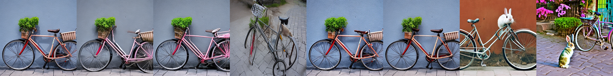
Spatial Prompt: “a rabbit near a bicycle”

Non-spatial Prompt: “A gardener is pruning a beautiful bonsai tree.”

Complex Prompt: “The white mug is on top of the black coaster.”

Figure 2: Qualitative samples for all categories.

5 Discussion

The self-supervised nature of our approach to fine-tuning, which solely relies on the t2i model for the generation of a synthetic candidate set of prompt-image pairs, is limited by the capabilities of the pre-trained model. Indeed, an underlying assumption we make is to expect the pre-trained model to eventually produce images that are aligned to the prompt, as done in previous works [73, 36]. Then, our information-theoretic alignment measure can be used to produce a useful fine-tuning set $\mathcal{S}$. However, in some cases (e.g., spatial or complex prompts) the pre-trained model can systematically fail in producing aligned samples. In this scenario, our method can be applied to existing t2i models that have been fine-tuned with complementary techniques, and substantially boost alignment performance, as we demonstrate in our experiments, as shown in Table 1.

In our work, we considered a large design space. In the context of fine-tuning approaches, we designed an alternative method to exploit pair-wise mi. Indeed, it is simple to rewrite the loss from Equation 1 to include a point-wise mi loss term, and use a small fraction of the t2i model training set to fine-tune it according to an “embedded” information-theoretic alignment measure. While this approach is in principle valid, we noticed that throughout the parameter optimization phase, mi estimates are affected by high variance, due to the poor quality of the unconditional denoising network of typical pre-trained t2i models [47]. Training the t2i model from scratch according to [47] can mitigate this issue, but defeats the purpose of using a pre-trained model.

Alternatively, we designed a variant of our method that operates at inference time, in a similar vein to the work in [13]. To do that, we blend the works [22, 41], to replace attention maps with pixel-level point-wise mi maps. Conditional sampling can then be amended as in [13]: we can define a new inference-time loss term that we use to update ${{\bm{{z}}}}_{t}$ on-the-fly, using information maps instead of cross-attention maps to steer model alignment. This is another valid approach that however bears the same problems discussed above: information maps quality suffers from a poorly trained unconditional denoising network, leading to poor results. Since the work in [41] does not explicitly focus on model alignment, the authors build information maps that use the unconditional denoising network with an edited prompt, instead of a null token, which is not an option for our study.

6 Conclusion

t2i alignment emerged as an important endeavor to steer image generation to follow the semantics and user intent expressed through a natural text prompt, as it can save considerable manual effort.

In this work, we presented a novel approach to measure alignment, that uses point-wise mi between prompt-image pairs to quantify the amount of information “flowing” between natural text and images. We demonstrated, both qualitatively and quantitatively, that pair-wise mi is coherent with existing alignment measures that either use external vqa models or human preference.

Armed with an information-theoretic measure of alignment, we presented mi-tune, a lightweight, self-supervised fine-tuning method that uses a pre-trained t2i model such as sd to estimate mi, and generates a synthetic set of aligned prompt-image pairs, which is then used in a parameter-efficient fine-tuning stage, to align the t2i model. Our approach does not require human annotation, auxiliary vqa models, nor costly inference-time techniques, and outperforms state-of-the-art approaches on most alignment categories examined in the literature.

Limitations. Accurate mi estimation is a difficult task, especially for high-dimensional, real-world data. For our method, mi estimation accuracy depends on the quality of the pre-trained denoising network of the base t2i model which, in the case of sd, is problematic for the unconditional version. As such, it is possible that mi-based alignment can suffer. Furthermore, despite mi appears to be more aligned to human preference than existing metrics, it is less interpretable when compared to methods that perform linguistic prompt analyses, or use auxiliary vqa models for explainability.

Finally, our information-theoretic alignment measure can be applied to arbitrary distributions, beyond text and images. Further work is necessary to demonstrate its application to other pre-trained models that operate on other modalities, such as e.g., the audio domain.

Broader impact. A valid concern to point out regarding our method mi-tune is that an improvement in the quality of generative models could be used to generate deepfakes for disinformation. Nevertheless, we believe that the positive impact of our work outweighs such problems.

[sections] [sections]l1

Appendix A Details on mi estimation

In this Section, we provide the proof for Equation 2.We start by recalling the definition of the forward and backward processes for a discrete-time diffusion model. For the forward process, we use the following Markov chain

$$q({{\bm{{z}}}}_{0:T},{{\bm{{p}}}})=q({{\bm{{z}}}}_{0},{{\bm{{p}}}})\prod\limits_{t=1}^{T}q({{\bm{{z}}}}_{t}\,|\,{{\bm{{z}}}}_{t-1}),\quad q({{\bm{{z}}}}_{t}\,|\,{{\bm{{z}}}}_{t-1})=\mathcal{N}({{\bm{{z}}}}_{t};\sqrt{1-\beta_{t}}{{\bm{{z}}}}_{t-1},\beta_{t}I)$$

The backward process (with or without a conditioning signal ${{\bm{{p}}}}$) evolves according to

$$p_{{{\bm{{\theta}}}}}({{\bm{{z}}}}_{0:T})=p({{\bm{{z}}}}_{T})\prod\limits_{t=1}^{T}p_{{{\bm{{\theta}}}}}({{\bm{{z}}}}_{t-1}\,|\,{{\bm{{z}}}}_{t}),\quad p_{{{\bm{{\theta}}}}}({{\bm{{z}}}}_{0:T}\,|\,{{\bm{{p}}}})=p({{\bm{{z}}}}_{T})\prod\limits_{t=1}^{T}p_{{{\bm{{\theta}}}}}({{\bm{{z}}}}_{t-1}\,|\,{{\bm{{z}}}}_{t},{{\bm{{p}}}})$$

where $p_{{{\bm{{\theta}}}}}({{\bm{{z}}}}_{t-1}\,|\,{{\bm{{z}}}}_{t})=\mathcal{N}({{\bm{{z}}}}_{t-1};\mu_{{\bm{{\theta}}}}({{\bm{{z}}}}_{t}),\beta_{t}I)$, with $\mu_{{\bm{{\theta}}}}({{\bm{{z}}}}_{t})=\frac{1}{\sqrt{\alpha_{t}}}\left({{\bm{{z}}}}_{t}-\frac{\beta_{t}}{\sqrt{1-\bar{\alpha}_{t}}}{{{\bm{{\epsilon}}}}}_{{\bm{{\theta}}}}({{\bm{{z}}}}_{t},t)\right)$. Similar expressions can be obtained for the conditional version.

Our goal here is to show that the following equality holds

$$\mathbb{E}_{{{\bm{{p}}}}}[\textsc{kl}\left[q({{\bm{{z}}}}_{0}\,|\,{{\bm{{p}}}})\;\|\;q({{\bm{{z}}}}_{0})\right]]=\mathbb{E}_{{{\bm{{z}}}},{{\bm{{p}}}}}[\textsc{I}({{\bm{{z}}}},{{\bm{{p}}}})],$$

which is the condition that $\textsc{I}({{\bm{{z}}}},{{\bm{{p}}}})$ of Equation 2 should satisfy to be a valid point-wise mi estimator. In particular, we will show that

$$\mathbb{E}_{{{\bm{{p}}}}}[\textsc{kl}\left[q({{\bm{{z}}}}_{0}\,|\,{{\bm{{p}}}})\;\|\;q({{\bm{{z}}}}_{0})\right]]=\mathbb{E}_{t,{{\bm{{p}}}},{{\bm{{z}}}},{{\bm{{\epsilon}}}}}\left[\kappa_{t}||{{\bm{{\epsilon}}}}_{{\bm{{\theta}}}}({{\bm{{z}}}}_{t},{{\bm{{p}}}},t)-{{\bm{{\epsilon}}}}_{{\bm{{\theta}}}}({{\bm{{z}}}}_{t},\emptyset,t)||^{2}\right],\,\,\,\kappa_{t}=\frac{\beta_{t}T}{2\alpha_{t}(1-\bar{\alpha}_{t})}.$$

To simplify our proof strategy, we consider the ideal case of perfect training, i.e., $p_{{{\bm{{\theta}}}}}({{\bm{{z}}}}_{0:T},{{\bm{{p}}}})=q({{\bm{{z}}}}_{0:T},{{\bm{{p}}}})$. Moreover, since $q({{\bm{{z}}}}_{t}\,|\,{{\bm{{z}}}}_{t-1},{{\bm{{p}}}})=q({{\bm{{z}}}}_{t}\,|\,{{\bm{{z}}}}_{t-1})$, we can rewrite the $\textsc{kl}\left[q({{\bm{{z}}}}_{0}\,|\,{{\bm{{p}}}})\;\|\;q({{\bm{{z}}}}_{0})\right]$ term as follows

$$\textsc{kl}\left[q({{\bm{{z}}}}_{0}\,|\,{{\bm{{p}}}})\;\|\;q({{\bm{{z}}}}_{0})\right]=\textsc{kl}\left[q({{\bm{{z}}}}_{0:T}\,|\,{{\bm{{p}}}})\;\|\;q({{\bm{{z}}}}_{0:T})\right]=\textsc{kl}\left[p_{{\bm{{\theta}}}}({{\bm{{z}}}}_{0:T}\,|\,{{\bm{{p}}}})\;\|\;p_{{{\bm{{\theta}}}}}({{\bm{{z}}}}_{0:T})\right]=$$

$$\int p_{{\bm{{\theta}}}}({{\bm{{z}}}}_{0:T}\,|\,{{\bm{{p}}}})\log\frac{p_{{\bm{{\theta}}}}({{\bm{{z}}}}_{0:T}\,|\,{{\bm{{p}}}})}{p_{{{\bm{{\theta}}}}}({{\bm{{z}}}}_{0:T})}\differential{{\bm{{z}}}}_{0:T}=\int p_{{\bm{{\theta}}}}({{\bm{{z}}}}_{0:T}\,|\,{{\bm{{p}}}})\sum\limits_{t=1}^{T}\log\frac{p_{{\bm{{\theta}}}}({{\bm{{z}}}}_{t-1}\,|\,{{\bm{{z}}}}_{t},{{\bm{{p}}}})}{p_{{{\bm{{\theta}}}}}({{\bm{{z}}}}_{t-1}\,|\,{{\bm{{z}}}}_{t})}\differential{{\bm{{z}}}}_{0:T}=$$

$$\sum\limits_{t=1}^{T}\int p_{{\bm{{\theta}}}}({{\bm{{z}}}}_{0:t-2,t:T}\,|\,{{\bm{{p}}}})\left(\int p_{{\bm{{\theta}}}}({{\bm{{z}}}}_{t-1}\,|\,{{\bm{{z}}}}_{t},{{\bm{{p}}}})\log\frac{p_{{\bm{{\theta}}}}({{\bm{{z}}}}_{t-1}\,|\,{{\bm{{z}}}}_{t},{{\bm{{p}}}})}{p_{{{\bm{{\theta}}}}}({{\bm{{z}}}}_{t-1}\,|\,{{\bm{{z}}}}_{t})}\differential{{\bm{{z}}}}_{t-1}\right)\differential{{\bm{{z}}}}_{0:t-2,t:T}=$$

$$\sum\limits_{t=1}^{T}\int p_{{\bm{{\theta}}}}({{\bm{{z}}}}_{t}\,|\,{{\bm{{p}}}})\textsc{kl}\left[p_{{\bm{{\theta}}}}({{\bm{{z}}}}_{t-1}\,|\,{{\bm{{z}}}}_{t},{{\bm{{p}}}})\;\|\;p_{{\bm{{\theta}}}}({{\bm{{z}}}}_{t-1}\,|\,{{\bm{{z}}}}_{t})\right]\differential{{\bm{{z}}}}_{t}=$$

$$\sum\limits_{t=1}^{T}\frac{1}{2\beta_{t}}\int p_{{\bm{{\theta}}}}({{\bm{{z}}}}_{t}\,|\,{{\bm{{p}}}})\norm{\mu_{{{\bm{{\theta}}}}}({{\bm{{z}}}}_{t})-\mu_{{{\bm{{\theta}}}}}({{\bm{{z}}}}_{t},{{\bm{{p}}}})}^{2}\differential{{\bm{{z}}}}_{t}=$$

$$\sum\limits_{t=1}^{T}\frac{1}{2\beta_{t}}\frac{\beta_{t}^{2}}{\alpha_{t}(1-\bar{\alpha}_{t})}\int p_{{\bm{{\theta}}}}({{\bm{{z}}}}_{t}\,|\,{{\bm{{p}}}})\norm{\epsilon_{{{\bm{{\theta}}}}}({{\bm{{z}}}}_{t})-\epsilon_{{{\bm{{\theta}}}}}({{\bm{{z}}}}_{t},{{\bm{{p}}}})}^{2}\differential{{\bm{{z}}}}_{t}=$$

$$\mathbb{E}_{t,{{\bm{{z}}}}_{t}}\left[\kappa_{t}\norm{\epsilon_{{{\bm{{\theta}}}}}({{\bm{{z}}}}_{t},\emptyset,t)-\epsilon_{{{\bm{{\theta}}}}}({{\bm{{z}}}}_{t},{{\bm{{p}}}},t)}^{2}\right]=$$

$$\mathbb{E}_{t,{{\bm{{z}}}},\epsilon}\left[\kappa_{t}\norm{\epsilon_{{{\bm{{\theta}}}}}({{\bm{{z}}}}_{t},\emptyset,t)-\epsilon_{{{\bm{{\theta}}}}}({{\bm{{z}}}}_{t},{{\bm{{p}}}},t)}^{2}\right],\quad\kappa_{t}=\frac{\beta_{t}T}{2\alpha_{t}(1-\bar{\alpha}_{t})}$$

which allows to prove that the quantity in Equation 2 is indeed a valid point-wise mi estimator.

Appendix B Details on user study

We now present our preliminary user study, which is based on focus groups only, with (lightly) guided discussions led by a moderator. Although it is easy to use the methodology described below to launch a large-scale survey campaign, this would require a completely different organization and implementation, which we did not put in place for this work.

The survey web app. Beside punctually comparing alignment metrics § 3 and methods § 4.4, we designed a web app to collect subjective feedback, in the form of mini surveys, from real users. Each survey is composed of multiple rounds, each showing a prompt and a set of images generated from it. Under the hood, the web app corresponds to a jupyter notebook with ipywidgets for UI controls, rendered via the voila framework and deployed live via a docker-ized HuggingFace space. Via the web app we run campaigns to compare alignment metrics and to compare alignment methods.

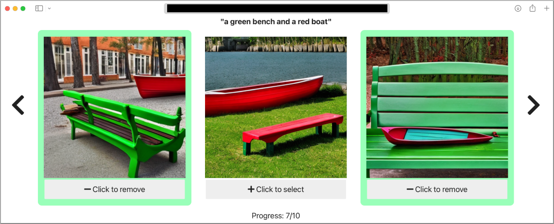
Figure 3: Web app screenshot example of the alignment metric comparison survey (URL blackened out for anonymization).

Fig. 3 shows an example screenshot of the alignment metric comparison survey. As from the example, users are free to select from 0 to up to 3 images for each prompt in the alignment metric comparison survey (0 to up to 8 for the alignment comparison survey). However, to stress users subjectivity, we intentionally did not provide guidelines on how to handle “odd” cases (e.g., if the prompt asks for a picture of “an apple”, but the picture show more than one apple). Last, each survey is saved as a separate CSV with the timestamp of its creation which also serves as unique identifier of the survey, i.e., neither user identification is required, nor cookies are set as part of the web app logic, so users’ privacy and anonymity is preserved.

Table 3: User study about comparing alignment metrics.

Metric			Campaign answers (%)
mi	blip-vqa	hps	Academic users	Random users	Students	avg
○	○	○	14.7	16.9	25.0	18.9
○	○	●	1.8	14.0	2.7	6.2
○	●	○	10.4	22.0	4.1	12.2
○	●	●	4.0	7.4	3.6	5.0
●	○	○	4.0	10.6	0.9	5.2
●	○	●	6.0	2.5	2.3	3.6
●	●	○	18.7	10.6	16.8	15.4
●	●	●	40.4	16.0	44.6	33.7
●	◑	◑	69.1	39.7	64.6	57.8
◑	●	◑	73.5	56.0	69.1	66.2
◑	◑	●	52.2	39.9	53.2	48.2

●(selected)     ○(not selected)     ◑ (indifferent to the selection)

B.1 Comparing alignment metrics.

In this analysis we aimed to understand how users perceive images selected via blip-vqa, hps and mi. To do so, we run surveys composed of 10 rounds, each showing a prompt and the related best image among 50 generations according to each metric. Each of the 10 prompts is randomly selected from a pool of 700 prompts for the color category, and at each round the order in which the 3 pictures is shown is also randomized.

We run surveys across three user groups: Academic users, counting 5 members, are representative of highly informed and tech savvy users, who are familiar with how generative models work; Random users, counting 25 members, are representative of illiterate users who are not familiar with computer-based image generation; Students, counting 16 members, are representative of masters’ level students who are familiar with image generation tools, and who have attended introductory-level machine learning classes.

Overall, we collected 45, 35 and 22 surveys across 3 days for Academics, Random users and Students respectively which we detail in Table 3. The top part of the table breaks down all possible answers combinations. The results, although with some differences between user groups, clearly highlight that the three alignment metrics we consider in this work are roughly equivalent, with mi and blip-vqa being preferred over hps. For the Academics and Students groups, all the three images are considered sufficiently aligned with the prompt in almost half of the cases ($40.4\%$ and $44.6\%$ respectively). Interestingly, random users select only one of the three images about 10$\times$ much more frequently than the other two groups (on average 14.2% for real users while 5.4% and 3% for Academics and Students respectively). We hypothesise that being previously exposed (or not) to the technical problems of image generation from the alignment perspective, or simply being literate about machine learning can influence the selection among the three pictures.

The bottom part of the table summarizes the answers for each individual metric. Despite the general preference for blip-vqa, the results corroborate once more that MI is a valid alignment measure, and that it is also compatible with aesthetics.

Finally, we recall that our goal in this section is to study whether mi is a plausible alignment measure, rather than electing the “best” alignment metric. Indeed, this analysis does not indicate the final performance of alignment methods, which instead we report in Table 1.

Table 4: Users study about comparing alignment methods. Bold indicates best performance; Underline indicates second-best performance; the symbol $\diamond$ indicates the best competing method in each category.

Alignment		Category (%)
Methodology	Model	Color	Shape	Texture	2D-Spatial	Non-spatial	Complex
none	sd-2.1-base	29.8	11.9	40.5	35.7	66.7	29.8
Inference-time	a&e	$\diamond$31.0	$\diamond$15.5	$\diamond$52.4	32.1	65.5	31.0
	sdg	26.2	15.4	38.1	38.1	61.9	29.8
	scg	20.2	11.9	33.3	$\diamond$40.5	$\diamond$69.0	$\diamond$39.3
Fine-tuning	dpok	23.8	16.7	$\diamond$47.6	34.5	$\diamond$70.2	$\diamond$38.1
	gors	$\diamond$34.5	14.3	48.8	$\diamond$36.9	65.5	31.0
	hn-itm	23.8	$\diamond$19.0	31.0	20.2	47.6	23.8
	mi-tune	46.4	25.0	51.2	45.2	73.8	46.4

B.2 Comparing alignment methods.

In this analysis we aimed to understand how users perceive images generated by the 8 methods we considered in our study, i.e., “vanilla” sd, a&e [13], sdg [21] and scg [72] dpok [19], gors [33], hn-itm [42] and our method mi-tune (when used with a single round of fine-tuning).

To do so, we run surveys composed of 12 rounds, i.e., 2 rounds for each category. Each round shows a prompt and the 8 pictures generated using a different method. For each category, we randomly selected 100 prompts from T2I-Combench test set to pre-generate the pictures. At run time, the web app randomly select 2 prompts for each category and randomly pics images from the related pool. Then it randomly arranges the rounds (so that categories are shuffled) and also the methods (so that pictures of a method are not visualized in the same order).

Table 4 collects the results of a campaign with 42 surveys. Specifically, the table shows the percentage of answers where the picture of a given method was selected (no matter if other methods were also selected). Overall, the results confirm what measured via BLIP-VQA in Table 1 – MI is a solid choice for model alignment.

Appendix C Experimental protocol details

We report in Table 5 all the hyper-parameters we used for our experiments.

Table 5: Training hyperparameters.

Name	Value
Trainable model	unet
Trainable timesteps	$t\sim U(500,1000)$
PEFT	DoRA [49]
Rank	$32$
$\alpha$	$32$
Learning rate (LR)	$1e-4$
Gradient norm clipping	$1.0$
LR scheduler	Constant
LR warmup steps	$0$
Optimizer	AdamW
AdamW - $\beta_{1}$	$0.9$
AdamW - $\beta_{2}$	$0.999$
AdamW - weight decay	$1e-2$
AdamW - $\epsilon$	$1e-8$
Resolution	$512\times 512$
Classifier-free guidance scale	7.5
Denoising steps	$50$
Batch size	400
Training iterations	300
GPUs for Training	1 $\times$ NVIDIA A100

Next, we provide additional details on the computational cost of mi-tune. In our approach, there are two distinct phases that require computational effort:

• The first is the construction of the fine-tuning set $\mathcal{S}$ based on point-wise mi. As a reminder, for this phase, we use a pre-trained sd model (at a resolution $512\times 512$) and, given a prompt, conditionally generate 50 images, while at the same time computing point-wise mi between the prompt and each image. This is done for all the prompts in the set $\mathcal{P}$, which counts 700 entries. In our experiments, on a single A100-80GB GPU, the generation of the fine-tuning set $\mathcal{S}$ requires roughly 24 hours.

• The second is the parameter efficient fine-tuning of the pre-trained model. Using the configuration discussed above, mi-tune requires 8 hours for the fine-tuning, on a single A100-80GB GPU.

Note that there is no overhead at image generation time: once a pre-trained model has been fine-tuned with mi-tune, conditional sampling takes the same amount of time of “vanilla” sd.

Appendix D Additional results and ablations

D.1 Ablation: Fine-tuning set size

In this Section, we provide additional details and ablations on the size and composition of the fine-tuning set $\mathcal{S}$.

There are two factors that determine both the quality and the associated computational cost related to the fine-tuning set $\mathcal{S}$: the number of candidate images $M$, out of which a given fraction $k/M$ is selected to be included in $\mathcal{S}$. Next, we analyze such trade-off. The baseline model mi-tune in Table 6 corresponds to result obtained by selecting the top $2\%$ images (1 out of 50) according to the mi metric. We repeated the finetuning experiments on the categories Color and Shape by varying the selection ratio in the ranges $\{7/50,1/30,1/100,1/500\}$. Results indicate that the best selection ratio is the middle-range corresponding to the baseline mi-tune. We hypothesise that higher selection ratios pollute the fine-tuning set with lower quality images, while a more selective threshold favours images which have the highest alignment but possibly lower realism. Additionally, we remark that the number $M$ of candidate images has a negligible impact, above $M=50$, whereas fewer candidate images induce degraded performance. Hence, the value $M=50$ is, in our experiments, a sweet-spot that produces a valid candidate set, while not imposing a large computational burden.

Table 6: blip-vqa-vqa alignment results on t2i-CompBench’s Color and Shape categories varying size and composition of fine-tuning set.

Model	Category
	Color	Shape
mi-tune-7out50	59.31	47.26
mi-tune-1out30	58.12	47.48
mi-tune-1out50	61.57	48.40
mi-tune-1out100	60.12	47.80
mi-tune-1out500	59.28	46.79

Next, another natural question to ask is whether the self-supervised fine-tuning method we suggest in this work is a valid strategy. Indeed, instead of using synthetic image data for fine-tuning the base model, it is also possible to use real-life, captioned image data. Then, we present an ablation on the use of real samples, along with synthetic images, in the fine-tuning procedure. In Table 7 we report the experimental results obtained by composing the fine-tuning dataset by $x\%$ generated images and $(1-x)\%$ of real images taken from the CC12M dataset [10], where in both cases we select, using mi, the candidate images to be used in the fine-tuning set $\mathcal{S}$. So, for example, mi-tune-Real0.25, indicates that we use 25% of real images. Interestingly, we observe the following trend. Complementing the synthetically generated samples with few, real ones, improves performance: this is akin to a regularization term which prevents the quality of the generated images to deviate too much from the quality of the real ones. However, increasing the fraction of real images can be detrimental.

Table 7: blip-vqa-vqa alignment results on t2i-CompBench’s Color and Shape categories finetuning using a mixture of generated and real images.

Model	Category
	Color	Shape
mi-tune	61.57	48.40
mi-tune-Real0.25	61.34	48.47
mi-tune-Real0.5	61.63	49.50
mi-tune-Real0.9	59.83	48.92

D.2 Ablation: Model fine-tuning

In this Section, we provide additional results (Table 8) on mi-tune, concerning which part of the pre-trained sd model to fine-tune. In particular, we have tried to fine-tune the denoising unet network alone and both the denoising and the text encoding (clip) networks. The baseline results are obtained, as described in the main paper, with Do-RA [49] adapters. Switching to Lo-RA layers [31] incurs in a performance degradation, a trend observed also for other tasks in the literature [49]. Interestingly, joint fine-tuning of the unet backbone together with the text encoder layers degrades performance as well, which has also been observed in the literature [33]. Even if, in principle, a joint fine-tuning strategy should provide better results, as the amount of information transferred from the prompt to the image is bottle-necked by the text encoder architecture, we observed empirically more unstable training dynamics than the variant where only the score network backbone is fine-tuned, resulting in degraded performance.

Table 8: blip-vqa-vqa alignment results on t2i-CompBench’s Color and Shape categories finetuning different portions of the model.

Model	Category
	Color	Shape
mi-tune-DoRA	61.57	48.40
mi-tune-LoRA	58.25	48.27
mi-tune-U+T(joint)	57.88	47.79

Appendix E Additional qualitative results

E.1 Color Binding Samples

sd

dpok

gors

hn-itm

a&e

sdg

scg

mi-tune

a black apple and a green backpack

a red apple and a green train

a blue bear and a brown boat

a green banana and a brown horse

a green bench and a blue bowl

a green bench and a blue bowl

a green banana and a red suitcase

a green banana and a red suitcase

a blue pencil and a yellow notebook

Figure 4: Color

E.2 Shape binding samples

sd

dpok

gors

hn-itm

a&e

sdg

scg

mi-tune

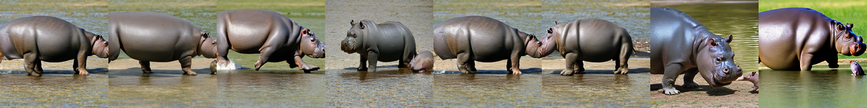
a big hippopotamus and a small mouse

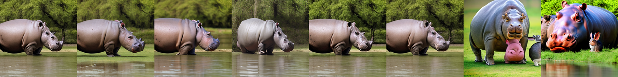
a big hippopotamus and a small rabbit

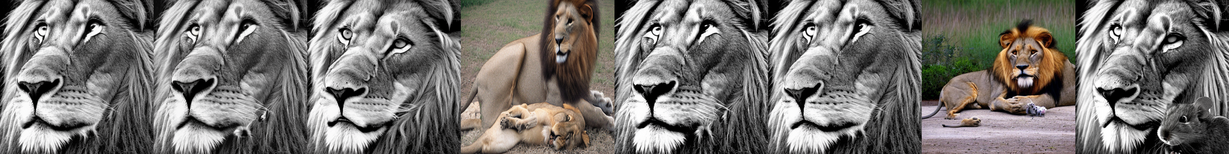
a big lion and a small mouse

a cubic block and a cylindrical jar of honey

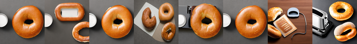
a round bagel and a rectangular toaster

an oval picture frame and a rectangular painting

an oval picture frame and a square painting

a big whale and a small dolphin

a cubic block and a cylindrical bottle

Figure 5: Shape

E.3 Texture binding samples

sd

dpok

gors

hn-itm

a&e

sdg

scg

mi-tune

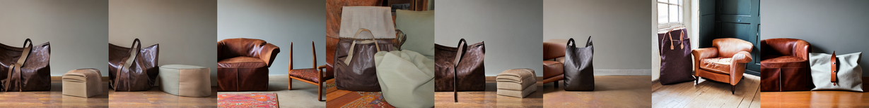
a fabric bag and a leather chair

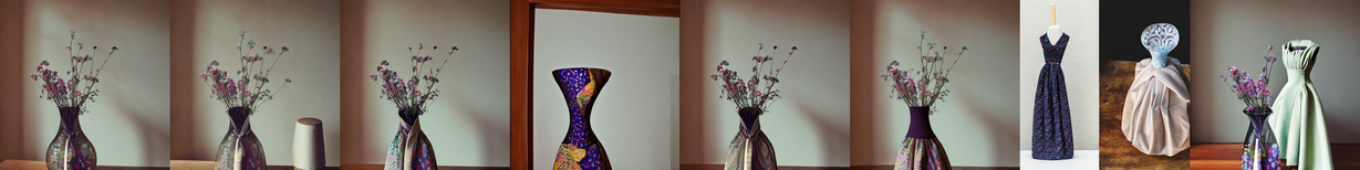
a fabric dress and a glass vase

a metallic desk lamp and a fluffy blanket

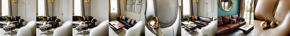
a metallic earring and a leather sofa

a plastic bottle and a leather wallet

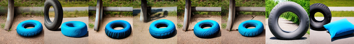
a rubber tire and a fabric pillow

a rubber tire and a metallic fork

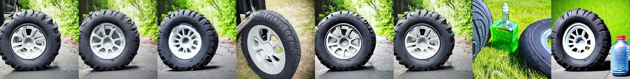
a rubber tire and a plastic bottle

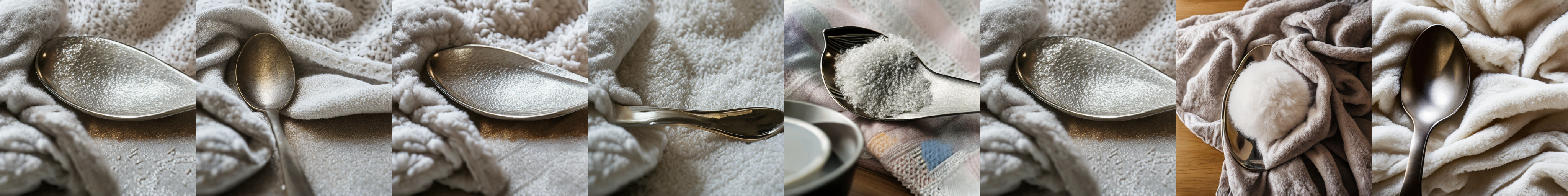
a metallic spoon and a fluffy blanket

Figure 6: Texture

E.4 Spatial prompts

sd

dpok

gors

hn-itm

a&e

sdg

scg

mi-tune

a bicycle on the top of a turtle

a bird on the top of a person

a chicken on the left of a girl

a clock on the top of a sheep

a cup on the right of a dog

a horse on side of a bicycle

a man on the right of a lamp

a sheep on the left of a lamp

a dog on the top of a desk

Figure 7: Spatial

E.5 Non-Spatial prompts

sd

dpok

gors

hn-itm

a&e

sdg

scg

mi-tune

A child is jumping on a trampoline in their backyard.

A gardener is pruning a beautiful bonsai tree.

A man is holding a soldering iron and repairing a broken electronic device.

A person is holding a pencil and sketching a portrait.

A person is practicing their juggling skills at the circus.

A woman is practicing her violin in her music room.

The paper crafter is making a paper flower bouquet.

A child is playing with a toy construction set and building a tower.

A child is playing with a toy construction set and building a tower.

Figure 8: Non-spatial

E.6 Complex prompts

sd

dpok

gors

hn-itm

a&e

sdg

scg

mi-tune

The red hat was on top of the brown coat.

The red hat was on top of the brown coat.

The red hat was on top of the brown coat.

The white mug is on top of the black coaster.

The striped rug was on top of the tiled floor.

The striped rug was on top of the tiled floor.

The sleek black laptop sat on the clean white desk.

The black chair was on the left of the white table.

The black chair was on the left of the white table.

Figure 9: Complex

References

- [1] Negative prompts. https://huggingface.co/spaces/stabilityai/stable-diffusion/discussions/7857, 2022.
- [2] Aishwarya Agarwal, Srikrishna Karanam, K J Joseph, Apoorv Saxena, Koustava Goswami, and Balaji Vasan Srinivasan. A-star: Test-time attention segregation and retention for text-to-image synthesis. In Proceedings of the IEEE/CVF International Conference on Computer Vision (ICCV), pages 2283–2293, October 2023.
- [3] Alexander A Alemi and Ian Fischer. Gilbo: One metric to measure them all. Advances in Neural Information Processing Systems, 31, 2018.
- [4] Alexander A Alemi, Ian Fischer, Joshua V Dillon, and Kevin Murphy. Deep variational information bottleneck. In International Conference on Learning Representations, 2016.
- [5] Yogesh Balaji, Seungjun Nah, Xun Huang, Arash Vahdat, Jiaming Song, Karsten Kreis, Miika Aittala, Timo Aila, Samuli Laine, Bryan Catanzaro, Tero Karras, and Ming-Yu Liu. ediff-i: Text-to-image diffusion models with ensemble of expert denoisers. arXiv preprint arXiv:2211.01324, 2022.
- [6] Yogesh Balaji, Seungjun Nah, Xun Huang, Arash Vahdat, Jiaming Song, Qinsheng Zhang, Karsten Kreis, Miika Aittala, Timo Aila, Samuli Laine, Bryan Catanzaro, Tero Karras, and Ming-Yu Liu. ediff-i: Text-to-image diffusion models with ensemble of expert denoisers. arXiv preprint arXiv:2211.01324, 2022.
- [7] Mohamed Ishmael Belghazi, Aristide Baratin, Sai Rajeshwar, Sherjil Ozair, Yoshua Bengio, Aaron Courville, and Devon Hjelm. Mutual information neural estimation. In Proceedings of the 35th International Conference on Machine Learning, 2018.
- [8] Anthony J Bell and Terrence J Sejnowski. An information-maximization approach to blind separation and blind deconvolution. Neural computation, 7(6):1129–1159, 1995.
- [9] Rob Brekelmans, Sicong Huang, Marzyeh Ghassemi, Greg Ver Steeg, Roger Baker Grosse, and Alireza Makhzani. Improving mutual information estimation with annealed and energy-based bounds. In International Conference on Learning Representations, 2022.
- [10] Soravit Changpinyo, Piyush Sharma, Nan Ding, and Radu Soricut. Conceptual 12m: Pushing web-scale image-text pre-training to recognize long-tail visual concepts. In Proceedings of the IEEE/CVF conference on computer vision and pattern recognition, pages 3558–3568, 2021.
- [11] Agneet Chatterjee, Gabriela Ben Melech Stan, Estelle Aflalo, Sayak Paul, Dhruba Ghosh, Tejas Gokhale, Ludwig Schmidt, Hannaneh Hajishirzi, Vasudev Lal, Chitta Baral, and Yezhou Yang. Getting it right: Improving spatial consistency in text-to-image models, 2024.
- [12] Hila Chefer, Yuval Alaluf, Yael Vinker, Lior Wolf, and Daniel Cohen-Or. Attend-and-excite: Attention-based semantic guidance for text-to-image diffusion models. ACM Trans. Graph., 42(4), 2023.
- [13] Hila Chefer, Yuval Alaluf, Yael Vinker, Lior Wolf, and Daniel Cohen-Or. Attend-and-excite: Attention-based semantic guidance for text-to-image diffusion models, 2023.
- [14] Xi Chen, Yan Duan, Rein Houthooft, John Schulman, Ilya Sutskever, and Pieter Abbeel. Infogan: Interpretable representation learning by information maximizing generative adversarial nets. Advances in neural information processing systems, 29, 2016.
- [15] Kevin Clark, Paul Vicol, Kevin Swersky, and David J. Fleet. Directly fine-tuning diffusion models on differentiable rewards. In The Twelfth International Conference on Learning Representations, 2024.
- [16] Colin Conwell and Tomer Ullman. Testing relational understanding in text-guided image generation, 2022.
- [17] Omer Dahary, Or Patashnik, Kfir Aberman, and Daniel Cohen-Or. Be yourself: Bounded attention for multi-subject text-to-image generation, 2024.
- [18] Prafulla Dhariwal and Alexander Nichol. Diffusion models beat gans on image synthesis. In M. Ranzato, A. Beygelzimer, Y. Dauphin, P.S. Liang, and J. Wortman Vaughan, editors, Advances in Neural Information Processing Systems, volume 34, pages 8780–8794. Curran Associates, Inc., 2021.
- [19] Ying Fan, Olivia Watkins, Yuqing Du, Hao Liu, Moonkyung Ryu, Craig Boutilier, Pieter Abbeel, Mohammad Ghavamzadeh, Kangwook Lee, and Kimin Lee. Reinforcement learning for fine-tuning text-to-image diffusion models. In Thirty-seventh Conference on Neural Information Processing Systems, 2023.
- [20] Weixi Feng, Xuehai He, Tsu-Jui Fu, Varun Jampani, Arjun Reddy Akula, Pradyumna Narayana, Sugato Basu, Xin Eric Wang, and William Yang Wang. Training-free structured diffusion guidance for compositional text-to-image synthesis. In The Eleventh International Conference on Learning Representations, 2023.
- [21] Weixi Feng, Xuehai He, Tsu-Jui Fu, Varun Jampani, Arjun Reddy Akula, Pradyumna Narayana, Sugato Basu, Xin Eric Wang, and William Yang Wang. Training-free structured diffusion guidance for compositional text-to-image synthesis. In The Eleventh International Conference on Learning Representations, 2023.
- [22] Giulio Franzese, Mustapha Bounoua, and Pietro Michiardi. MINDE: Mutual information neural diffusion estimation. In The Twelfth International Conference on Learning Representations, 2024.
- [23] Oran Gafni, Adam Polyak, Oron Ashual, Shelly Sheynin, Devi Parikh, and Yaniv Taigman. Make-a-scene: Scene-based text-to-image generation with human priors, 2022.
- [24] Brian Gordon, Yonatan Bitton, Yonatan Shafir, Roopal Garg, Xi Chen, Dani Lischinski, Daniel Cohen-Or, and Idan Szpektor. Mismatch quest: Visual and textual feedback for image-text misalignment, 2023.
- [25] Paul Grimal, Hervé Le Borgne, Olivier Ferret, and Julien Tourille. Tiam - a metric for evaluating alignment in text-to-image generation. In Proceedings of the IEEE/CVF Winter Conference on Applications of Computer Vision (WACV), pages 2890–2899, January 2024.
- [26] Jack Hessel, Ari Holtzman, Maxwell Forbes, Ronan Le Bras, and Yejin Choi. CLIPScore: A reference-free evaluation metric for image captioning. In Proceedings of the 2021 Conference on Empirical Methods in Natural Language Processing, 2021.
- [27] R Devon Hjelm, Alex Fedorov, Samuel Lavoie-Marchildon, Karan Grewal, Phil Bachman, Adam Trischler, and Yoshua Bengio. Learning deep representations by mutual information estimation and maximization. In International Conference on Learning Representations, 2019.
- [28] Jonathan Ho, Ajay Jain, and Pieter Abbeel. Denoising diffusion probabilistic models. In Advances in Neural Information Processing Systems, volume 33, pages 6840–6851, 2020.
- [29] Jonathan Ho and Tim Salimans. Classifier-free diffusion guidance. In NeurIPS 2021 Workshop on Deep Generative Models and Downstream Applications, 2021.
- [30] Jonathan Ho and Tim Salimans. Classifier-free diffusion guidance. arXiv preprint arXiv:2207.12598, 2022.
- [31] Edward J. Hu, Yelong Shen, Phillip Wallis, Zeyuan Allen-Zhu, Yuanzhi Li, Shean Wang, Lu Wang, and Weizhu Chen. Lora: Low-rank adaptation of large language models, 2021.
- [32] Yushi Hu, Benlin Liu, Jungo Kasai, Yizhong Wang, Mari Ostendorf, Ranjay Krishna, and Noah A. Smith. Tifa: Accurate and interpretable text-to-image faithfulness evaluation with question answering. In Proceedings of the IEEE/CVF International Conference on Computer Vision (ICCV), pages 20406–20417, October 2023.
- [33] Kaiyi Huang, Kaiyue Sun, Enze Xie, Zhenguo Li, and Xihui Liu. T2i-compbench: A comprehensive benchmark for open-world compositional text-to-image generation. In Thirty-seventh Conference on Neural Information Processing Systems Datasets and Benchmarks Track, 2023.
- [34] Sicong Huang, Alireza Makhzani, Yanshuai Cao, and Roger Grosse. Evaluating lossy compression rates of deep generative models. In International Conference on Machine Learning. PMLR, 2020.
- [35] Wonjun Kang, Kevin Galim, and Hyung Il Koo. Counting guidance for high fidelity text-to-image synthesis, 2023.
- [36] Shyamgopal Karthik, Karsten Roth, Massimiliano Mancini, and Zeynep Akata. If at first you don’t succeed, try, try again: Faithful diffusion-based text-to-image generation by selection. arXiv preprint arXiv:2305.13308, 2023.
- [37] M. G. Kendall. A Ner Measure of Rank Correlation. Biometrika, 30(1-2):81–93, 06 1938.
- [38] Yunji Kim, Jiyoung Lee, Jin-Hwa Kim, Jung-Woo Ha, and Jun-Yan Zhu. Dense text-to-image generation with attention modulation. In ICCV, 2023.
- [39] Diederik P Kingma, Tim Salimans, Ben Poole, and Jonathan Ho. Variational diffusion models. In A. Beygelzimer, Y. Dauphin, P. Liang, and J. Wortman Vaughan, editors, Advances in Neural Information Processing Systems, 2021.
- [40] Alexander Kirillov, Eric Mintun, Nikhila Ravi, Hanzi Mao, Chloe Rolland, Laura Gustafson, Tete Xiao, Spencer Whitehead, Alexander C. Berg, Wan-Yen Lo, Piotr Dollar, and Ross Girshick. Segment anything. In Proceedings of the IEEE/CVF International Conference on Computer Vision (ICCV), pages 4015–4026, October 2023.
- [41] Xianghao Kong, Ollie Liu, Han Li, Dani Yogatama, and Greg Ver Steeg. Interpretable diffusion via information decomposition. In The Twelfth International Conference on Learning Representations, 2024.
- [42] Benno Krojer, Elinor Poole-Dayan, Vikram Voleti, Christopher Pal, and Siva Reddy. Are diffusion models vision-and-language reasoners? arXiv preprint arXiv:2305.16397, 2023.
- [43] Kimin Lee, Hao Liu, Moonkyung Ryu, Olivia Watkins, Yuqing Du, Craig Boutilier, Pieter Abbeel, Mohammad Ghavamzadeh, and Shixiang Shane Gu. Aligning text-to-image models using human feedback, 2023.
- [44] Nunzio A Letizia and Andrea M Tonello. Copula density neural estimation. arXiv preprint arXiv:2211.15353, 2022.
- [45] Junnan Li, Dongxu Li, Silvio Savarese, and Steven Hoi. Blip-2: bootstrapping language-image pre-training with frozen image encoders and large language models. In Proceedings of the 40th International Conference on Machine Learning, 2023.
- [46] Yumeng Li, Margret Keuper, Dan Zhang, and Anna Khoreva. Divide & bind your attention for improved generative semantic nursing. In 34th British Machine Vision Conference 2023, BMVC 2023, 2023.
- [47] Shanchuan Lin and Xiao Yang. Diffusion model with perceptual loss, 2024.
- [48] Nan Liu, Shuang Li, Yilun Du, Antonio Torralba, and Joshua B. Tenenbaum. Compositional visual generation with composable diffusion models. In Computer Vision – ECCV 2022: 17th European Conference, Tel Aviv, Israel, October 23–27, 2022, Proceedings, Part XVII, page 423–439, 2022.
- [49] Shih-Yang Liu, Chien-Yi Wang, Hongxu Yin, Pavlo Molchanov, Yu-Chiang Frank Wang, Kwang-Ting Cheng, and Min-Hung Chen. Dora: Weight-decomposed low-rank adaptation, 2024.
- [50] Vivian Liu and Lydia B Chilton. Design guidelines for prompt engineering text-to-image generative models. In Proceedings of the 2022 CHI Conference on Human Factors in Computing Systems, 2022.
- [51] Jian Ma, Junhao Liang, Chen Chen, and Haonan Lu. Subject-diffusion:open domain personalized text-to-image generation without test-time fine-tuning, 2023.
- [52] David JC MacKay. Information theory, inference and learning algorithms. Cambridge university press, 2003.
- [53] Shweta Mahajan, Tanzila Rahman, Kwang Moo Yi, and Leonid Sigal. Prompting hard or hardly prompting: Prompt inversion for text-to-image diffusion models, 2023.
- [54] Oscar Mañas, Pietro Astolfi, Melissa Hall, Candace Ross, Jack Urbanek, Adina Williams, Aishwarya Agrawal, Adriana Romero-Soriano, and Michal Drozdzal. Improving text-to-image consistency via automatic prompt optimization, 2024.
- [55] David McAllester and Karl Stratos. Formal limitations on the measurement of mutual information. In International Conference on Artificial Intelligence and Statistics, 2020.
- [56] Tuna Han Salih Meral, Enis Simsar, Federico Tombari, and Pinar Yanardag. Conform: Contrast is all you need for high-fidelity text-to-image diffusion models. In Proceedings of the IEEE/CVF Conference on Computer Vision and Pattern Recognition, 2024.
- [57] Alex Nichol, Prafulla Dhariwal, Aditya Ramesh, Pranav Shyam, Pamela Mishkin, Bob McGrew, Ilya Sutskever, and Mark Chen. Glide: Towards photorealistic image generation and editing with text-guided diffusion models, 2022.
- [58] Michael Ogezi and Ning Shi. Optimizing negative prompts for enhanced aesthetics and fidelity in text-to-image generation, 2024.
- [59] Bernt Øksendal. Stochastic differential equations. Springer, 2003.
- [60] Aaron van den Oord, Yazhe Li, and Oriol Vinyals. Representation learning with contrastive predictive coding. Advances in neural information processing systems, 2018.
- [61] OpenAI. Chatgpt (gpt-4) [large language model], 2024.
- [62] Liam Paninski. Estimation of entropy and mutual information. Neural computation, 15(6):1191–1253, 2003.
- [63] George Papamakarios, Theo Pavlakou, and Iain Murray. Masked autoregressive flow for density estimation. Advances in neural information processing systems, 30, 2017.
- [64] Dustin Podell, Zion English, Kyle Lacey, Andreas Blattmann, Tim Dockhorn, Jonas Müller, Joe Penna, and Robin Rombach. SDXL: Improving latent diffusion models for high-resolution image synthesis. In The Twelfth International Conference on Learning Representations, 2024.
- [65] Alec Radford, Jong Wook Kim, Chris Hallacy, Aditya Ramesh, Gabriel Goh, Sandhini Agarwal, Girish Sastry, Amanda Askell, Pamela Mishkin, Jack Clark, Gretchen Krueger, and Ilya Sutskever. Learning transferable visual models from natural language supervision. In Proceedings of the 38th International Conference on Machine Learning, volume 139, pages 8748–8763, 2021.
- [66] Aditya Ramesh, Prafulla Dhariwal, Alex Nichol, Casey Chu, and Mark Chen. Hierarchical text-conditional image generation with clip latents, 2022.
- [67] Royi Rassin, Eran Hirsch, Daniel Glickman, Shauli Ravfogel, Yoav Goldberg, and Gal Chechik. Linguistic binding in diffusion models: Enhancing attribute correspondence through attention map alignment. In Thirty-seventh Conference on Neural Information Processing Systems, 2023.
- [68] Benjamin Rhodes, Kai Xu, and Michael U Gutmann. Telescoping density-ratio estimation. Advances in neural information processing systems, 2020.
- [69] Robin Rombach, Andreas Blattmann, Dominik Lorenz, Patrick Esser, and Björn Ommer. High-resolution image synthesis with latent diffusion models. In Proceedings of the IEEE/CVF Conference on Computer Vision and Pattern Recognition (CVPR), pages 10684–10695, June 2022.
- [70] Olaf Ronneberger, Philipp Fischer, and Thomas Brox. U-net: Convolutional networks for biomedical image segmentation. In Medical Image Computing and Computer-Assisted Intervention – MICCAI 2015, pages 234–241, 2015.
- [71] Chitwan Saharia, William Chan, Saurabh Saxena, Lala Li, Jay Whang, Emily L Denton, Kamyar Ghasemipour, Raphael Gontijo Lopes, Burcu Karagol Ayan, Tim Salimans, Jonathan Ho, David J Fleet, and Mohammad Norouzi. Photorealistic text-to-image diffusion models with deep language understanding. In Advances in Neural Information Processing Systems, volume 35, pages 36479–36494, 2022.
- [72] Tim Salimans and Jonathan Ho. Progressive distillation for fast sampling of diffusion models, 2022.
- [73] Dvir Samuel, Rami Ben-Ari, Simon Raviv, Nir Darshan, and Gal Chechik. Generating images of rare concepts using pre-trained diffusion models. 2024.
- [74] Claude Elwood Shannon. A mathematical theory of communication. The Bell system technical journal, 27(3):379–423, 1948.
- [75] Jascha Sohl-Dickstein, Eric Weiss, Niru Maheswaranathan, and Surya Ganguli. Deep unsupervised learning using nonequilibrium thermodynamics. In Proceedings of the 32nd International Conference on Machine Learning, volume 37, pages 2256–2265, 2015.
- [76] Jiaming Song and Stefano Ermon. Understanding the limitations of variational mutual information estimators. In International Conference on Learning Representations, 2019.
- [77] Yang Song and Stefano Ermon. Generative modeling by estimating gradients of the data distribution. In H. Wallach, H. Larochelle, A. Beygelzimer, F. d’ Alché-Buc, E. Fox, and R. Garnett, editors, Advances in Neural Information Processing Systems, volume 32. Curran Associates, Inc., 2019.
- [78] Yang Song and Stefano Ermon. Improved techniques for training score-based generative models. In H. Larochelle, M. Ranzato, R. Hadsell, M.F. Balcan, and H. Lin, editors, Advances in Neural Information Processing Systems, volume 33, pages 12438–12448. Curran Associates, Inc., 2020.
- [79] Yang Song, Jascha Sohl-Dickstein, Diederik P Kingma, Abhishek Kumar, Stefano Ermon, and Ben Poole. Score-based generative modeling through stochastic differential equations. In International Conference on Learning Representations, 2021.
- [80] Karl Stratos. Mutual information maximization for simple and accurate part-of-speech induction. In Proceedings of the 2019 Conference of the North American Chapter of the Association for Computational Linguistics: Human Language Technologies, Volume 1 (Long and Short Papers), 2019.
- [81] Jiao Sun, Deqing Fu, Yushi Hu, Su Wang, Royi Rassin, Da-Cheng Juan, Dana Alon, Charles Herrmann, Sjoerd van Steenkiste, Ranjay Krishna, and Cyrus Rashtchian. Dreamsync: Aligning text-to-image generation with image understanding feedback, 2023.
- [82] Raphael Tang, Linqing Liu, Akshat Pandey, Zhiying Jiang, Gefei Yang, Karun Kumar, Pontus Stenetorp, Jimmy Lin, and Ferhan Ture. What the DAAM: Interpreting stable diffusion using cross attention. In Proceedings of the 61st Annual Meeting of the Association for Computational Linguistics (Volume 1: Long Papers), pages 5644–5659, July 2023.
- [83] Bram Wallace, Meihua Dang, Rafael Rafailov, Linqi Zhou, Aaron Lou, Senthil Purushwalkam, Stefano Ermon, Caiming Xiong, Shafiq Joty, and Nikhil Naik. Diffusion model alignment using direct preference optimization, 2023.
- [84] Zijie J. Wang, Evan Montoya, David Munechika, Haoyang Yang, Benjamin Hoover, and Duen Horng Chau. DiffusionDB: A large-scale prompt gallery dataset for text-to-image generative models. In Proceedings of the 61st Annual Meeting of the Association for Computational Linguistics (Volume 1: Long Papers), 2023.
- [85] Zirui Wang, Zhizhou Sha, Zheng Ding, Yilin Wang, and Zhuowen Tu. Tokencompose: Grounding diffusion with token-level supervision, 2023.
- [86] Sam Witteveen and Martin Andrews. Investigating prompt engineering in diffusion models, 2022.
- [87] Qiucheng Wu, Yujian Liu, Handong Zhao, Trung Bui, Zhe Lin, Yang Zhang, and Shiyu Chang. Harnessing the spatial-temporal attention of diffusion models for high-fidelity text-to-image synthesis. In Proceedings of the IEEE/CVF International Conference on Computer Vision (ICCV), pages 7766–7776, October 2023.
- [88] Xiaoshi Wu, Yiming Hao, Keqiang Sun, Yixiong Chen, Feng Zhu, Rui Zhao, and Hongsheng Li. Human preference score v2: A solid benchmark for evaluating human preferences of text-to-image synthesis, 2023.
- [89] Xiaoshi Wu, Keqiang Sun, Feng Zhu, Rui Zhao, and Hongsheng Li. Human preference score: Better aligning text-to-image models with human preference, 2023.
- [90] Jiazheng Xu, Xiao Liu, Yuchen Wu, Yuxuan Tong, Qinkai Li, Ming Ding, Jie Tang, and Yuxiao Dong. Imagereward: Learning and evaluating human preferences for text-to-image generation. In Thirty-seventh Conference on Neural Information Processing Systems, 2023.
- [91] Huizhuo Yuan, Zixiang Chen, Kaixuan Ji, and Quanquan Gu. Self-play fine-tuning of diffusion models for text-to-image generation, 2024.
- [92] Shengjia Zhao, Jiaming Song, and Stefano Ermon. A lagrangian perspective on latent variable generative models. In Proc. 34th Conference on Uncertainty in Artificial Intelligence, 2018.
- [93] Xingyi Zhou, Vladlen Koltun, and Philipp Krähenbühl. Simple multi-dataset detection. In CVPR, 2022.
- [94] Deyao Zhu, Jun Chen, Xiaoqian Shen, Xiang Li, and Mohamed Elhoseiny. MiniGPT-4: Enhancing vision-language understanding with advanced large language models. In The Twelfth International Conference on Learning Representations, 2024.
[sections] \printcontents[sections]l1