Fast Bayesian Basis Selection for Functional Data Representation with Correlated Errors

Abstract

Functional data analysis (FDA) finds widespread application across various fields, due to data being recorded continuously over a time interval or at several discrete points. Since the data is not observed at every point but rather across a dense grid, smoothing techniques are often employed to convert the observed data into functions. In this work, we propose a novel Bayesian approach for selecting basis functions for smoothing one or multiple curves simultaneously. Our method differentiates from other Bayesian approaches in two key ways: (i) by accounting for correlated errors and (ii) by developing a variational EM algorithm instead of a Gibbs sampler. Simulation studies demonstrate that our method effectively identifies the true underlying structure of the data across various scenarios and it is applicable to different types of functional data. Our variational EM algorithm not only recovers the basis coefficients and the correct set of basis functions but also estimates the existing within-curve correlation. When applied to the motorcycle dataset, our method demonstrates comparable, and in some cases superior, performance in terms of adjusted $R^{2}$ compared to other techniques such as regression splines, Bayesian LASSO and LASSO. Additionally, when assuming independence among observations within a curve, our method, utilizing only a variational Bayes algorithm, is in the order of thousands faster than a Gibbs sampler on average. Our proposed method is implemented in R and codes are available at https://github.com/acarolcruz/VB-Bases-Selection.

1 Introduction

In Functional Data Analysis (FDA), a common problem involves assessing observations from a continuous functional $y(\cdot)$ at specific evaluation points, usually representing a continuous variable such as time. Since $y(\cdot)$ is not observed at every point but rather across a dense grid, smoothing techniques are often employed to convert the observed data into functions. This process, known as functional data representation, is commonly achieved using basis function expansion methods, considering, for example, Fourier and B-splines basis functions.

One common method for estimating a smooth function, which is represented by a linear combination of known basis functions, involves finding the set coefficients for this linear combination that minimizes a penalized least squares criterion. This criterion includes a penalty term that measures the function’s roughness. The smoothing parameter, which controls the trade-off between data fit and smoothness, is typically determined through cross-validation (Ramsay and Silverman,, 2005). However, while these methods effectively manage smoothness, they do not perform basis selection, which is the process of identifying the most relevant basis functions from a set of candidates.

Bayesian techniques have significantly advanced the field of functional data representation, providing robust and flexible modelling methods. For example, Gaussian processes, which are non-parametric models, are widely used in Bayesian functional data analysis due to their ability to model and smooth complex data (Williams and Rasmussen,, 2006). Additionally, spike-and-slab priors are employed for basis function selection, offering an effective approach to distinguish between relevant and irrelevant basis functions (Kuo and Mallick,, 1998; Ishwaran and Rao,, 2005; Crainiceanu et al.,, 2009; Sousa et al.,, 2024). For instance, Sousa et al., (2024) utilized spike-and-slab priors for simultaneous basis selection across multiple curves by introducing a hierarchical model and sampling from the posterior distribution via a Gibbs sampler.

Independence across observations within a curve is often assumed when performing functional data representation, as it greatly simplifies model inference derivation. However, this assumption may not hold true in certain scenarios, especially when working with repeated measurements or longitudinal data (Goldsmith et al.,, 2011; Huo et al.,, 2023). As a result, ignoring the data correlation structure can lead to inaccurate inference results (see Figure 1). Under a Bayesian framework, introducing a correlation structure within a curve poses a challenge in deriving the posterior distribution for the correlation parameters due to its non-conjugacy in most proposed structure cases. The incorporation of a data correlation structure often requires additional steps within the chosen Bayesian inference algorithm to address this issue. For instance, Dias et al., (2013) employed the Metropolis-Hastings method within a Gibbs sampler to account for non-conjugacy when estimating a correlation function decay parameter.

The use of Markov chain Monte Carlo (MCMC) methods, such as the Gibbs sampler, for basis function selection in functional data representation, as shown in Sousa et al., (2024), can be computationally costly, especially in large data settings. Therefore, considering alternative Bayesian inference approaches, such as variational inference, may yield more computationally efficient results (Goldsmith et al.,, 2011; Earls and Hooker,, 2017; Huo et al.,, 2023; Xian et al.,, 2024). Variational inference algorithms, such as variational Bayes (VB) or variational EM (Blei et al.,, 2017; Li and Ma,, 2023; Huo et al.,, 2023), aim to find the so-called variational distribution that best approximates the true posterior instead of sampling from the posterior distribution as MCMC techniques. Additionally, when performing basis selection for functional data representation, it is important to recognize that the assumption of independence across observations within a curve may not hold true in many situations.

Thus, in this work, we propose a novel Bayesian approach for selecting basis functions for smoothing one or multiple curves simultaneously. Our approach builds upon the method proposed by Sousa et al., (2024) in two key ways: (i) by accounting for correlated errors and (ii) by developing a variational EM algorithm instead of a Gibbs sampler. Since our main interest lies in basis function selection, we focus on obtaining a point estimate for a proposed correlation decay parameter while still approximating the full posterior distributions for the other model parameters. In the E-step of our variational EM algorithm, we fix the correlation decay parameter and estimate the variational distributions for the other model parameters using VB. In the subsequent M-step, we use these VB estimates to maximize the evidence lower bound (ELBO) with respect to the correlation decay parameter. The algorithm iterates until ELBO convergence. As a result, all model parameters are obtained simultaneously and automatically, facilitating for a rapid and adaptive selection of basis functions while incorporating a data correlation structure. Our proposed method is implemented in R and codes are available at https://github.com/acarolcruz/VB-Bases-Selection.

This paper is organized as follows: Section 2 provides an overview of variational inference, along with a detailed description of our proposed model and VB algorithm. Section 3 presents the results of simulation studies designed to evaluate the performance of our method under various scenarios. In Section 4, we apply our methodology to a real dataset, showcasing its practical utility. Finally, Section 5 offers a conclusion of our study and discusses the implications of our proposed method.

2 Methods

2.1 Variational Bayes

Unlike MCMC methods that approximate the exact posterior distribution by sampling from the stationary distribution of the model parameters, variational inference takes on an optimization approach for approximating probability densities (Jordan et al.,, 1999; Wainwright et al.,, 2008). Variational Bayes (VB) is a variational inference algorithm that approximates the posterior by another density restricted to a family with some desired properties (Blei et al.,, 2017). The approximated posterior is determined by the density in that family that minimizes the Kulback-Leibler (KL) divergence to the exact posterior. Let $\boldsymbol{\theta}$ be the set of model parameters, $q\in\mathcal{Q}$ be a density function over $\Theta$ (parameter space), and $\boldsymbol{y}$ be the observed data. Then, more precisely, VB seeks to find a variational distribution $q^{*}$ in $\mathcal{Q}$ that minimizes the KL divergence to the true posterior, that is,

$$q^{*}(\boldsymbol{\theta})=\operatorname*{arg\,min}_{q\in\mathcal{Q}}\operatorname*{KL}(q(\boldsymbol{\theta})\parallel p(\boldsymbol{\theta}\mid\boldsymbol{y})).$$ (1)

The KL divergence between the two densities is defined as:

$$\operatorname*{KL}(q(\boldsymbol{\theta})\parallel p(\boldsymbol{\theta}\mid\boldsymbol{y})) =\operatorname*{E}\left(\log\frac{q(\boldsymbol{\theta})}{p(\boldsymbol{\theta}\mid\boldsymbol{y})}\right)$$

$$=\operatorname*{E}(\log q(\boldsymbol{\theta}))-\operatorname*{E}(\log p(\boldsymbol{\theta}\mid\boldsymbol{y}))$$

$$=\operatorname*{E}(\log q(\boldsymbol{\theta}))-\operatorname*{E}(\log p(\boldsymbol{\theta},\boldsymbol{y}))+\log p(\boldsymbol{y}),$$ (2)

where all expectations are taken with respect to $q(\boldsymbol{\theta})$. Directly minimizing $\operatorname*{KL}(q\parallel p)$ is not possible since $p(\boldsymbol{y})$ is often intractable to compute. As an alternative, since $\log p(\boldsymbol{y})$ is considered a constant with respect to $q(\boldsymbol{\theta})$ and $\operatorname*{KL}(q\parallel p)$ is non-negative, we optimize an alternative objective function called the evidence lower bound (ELBO). The ELBO is derived from the decomposition of $\log p(\boldsymbol{y})$ as follows:

$$\log p(\boldsymbol{y}) =\log p(\boldsymbol{y})\int_{\Theta}q(\boldsymbol{\theta})d\boldsymbol{\theta}$$

$$=\int_{\Theta}\log\left\{\frac{p(\boldsymbol{\theta},\boldsymbol{y})/q(\boldsymbol{\theta})}{p(\boldsymbol{\theta}\mid\boldsymbol{y})/q(\boldsymbol{\theta})}\right\}q(\boldsymbol{\theta})d\boldsymbol{\theta}$$

$$=\int_{\Theta}q(\boldsymbol{\theta})\log\left[\frac{p(\boldsymbol{\theta},\boldsymbol{y})}{q(\boldsymbol{\theta})}\right]d\boldsymbol{\theta}+\int_{\Theta}q(\boldsymbol{\theta})\log\left[\frac{q(\boldsymbol{\theta})}{p(\boldsymbol{\theta}\mid\boldsymbol{y})}\right]d\boldsymbol{\theta}$$

$$=\operatorname*{KL}(q(\boldsymbol{\theta})\parallel p(\boldsymbol{\theta}\mid\boldsymbol{y}))+\underbrace{\int_{\Theta}q(\boldsymbol{\theta})\log\left[\frac{q(\boldsymbol{\theta})}{p(\boldsymbol{\theta}\mid\boldsymbol{y})}\right]d\boldsymbol{\theta}}_{ELBO}.$$ (3)

This decomposition demonstrates that the ELBO is the negative KL divergence presented in (2.1) plus $\log p(\boldsymbol{y})$. Therefore, maximizing the ELBO is equivalent to minimizing the KL divergence. Consequently, the task of approximating the posterior density with VB becomes an optimization problem, with the complexity determined by the choice of the density family $\mathcal{Q}$. One widely used family is the mean-field variational family, where the parameters $\boldsymbol{\theta}$ are assumed to be mutually independent, leading to the factorization $q(\boldsymbol{\theta})=\prod_{i}q_{i}(\theta_{i})$. This assumption facilitates the analytical computation of $q(\boldsymbol{\theta})$.

To obtain each variational distribution $q_{j}(\theta_{j})$ we consider the coordinate ascent variational inference (CAVI) algorithm (Bishop,, 2006). Under the CAVI, we optimize the ELBO with respect to a single variational density $q_{j}(\theta_{j})$ while holding the others fixed, resulting in the optimal variational distribution $q_{j}^{*}(\theta_{j})$ defined as follows:

$$\log q_{j}^{*}(\theta_{j})=E_{q(\boldsymbol{\theta}_{-j})}\Big{[}\log p(\boldsymbol{y},\boldsymbol{\theta})\Big{]}+\text{constant},$$ (4)

where $q(\boldsymbol{\theta}_{-j})$ indicates that the expectation is taken with respect to the variational distributions of all other model parameters except $\theta_{j}$ and “constant” represents any terms that do not depend on $\theta_{j}$.

2.2 Variational EM

Suppose that $\theta_{l}\in\Theta$ is a hyperparameter whose posterior distribution is intractable to obtain due to its non-conjugacy. In variational inference, one approach commonly used to address this issue is the Variational EM algorithm (Liu et al.,, 2019; Li and Ma,, 2023; Huo et al.,, 2023). Let $\Lambda\subset\Theta$ represents the set of model parameters for which we can approximate the posterior distribution using VB. The Variational EM algorithm iteratively maximizes the ELBO with respect to $q(\Lambda)$ and $\theta_{l}$ using the following two steps:

• E-step: Assuming $\theta_{l}$ fixed, we obtain the variational distribution of $q(\Lambda)$, $q^{*}(\Lambda)$, using the CAVI algorithm as described in Section 2.1;

• M-step: We compute the update of $\theta_{l}$ as the $\operatorname*{arg\,max}_{\theta_{l}}$ ELBO$(q^{*}(\Lambda),\theta_{l})$, where the obtained $q^{*}(\Lambda)$ in the E-step is held fixed.

2.3 Model

We consider the Bayesian model framework for basis selection as in Sousa et al., (2024) and demonstrate a Variational Bayes approach for approximate inference while incorporating a correlation structure into the data. Suppose there are $m$ curves, each with $n_{i}$ observations at points $t_{ij}\in A\subseteq\mathbb{R}$, where $i\in{1,\ldots,m}$ and $j\in{1,\ldots,n_{i}}$. Denote the observed value of the $i$-th curve at $t_{ij}$ as $y_{ij}$. We can express $y_{ij}$ as follows:

$$y_{ij}\equiv y_{i}(t_{ij})=g_{i}(t_{ij})+\varepsilon_{i}(t_{ij}),$$ (5)

where $g_{i}(t_{ij})$ is represented as a linear combination of $K$ known basis functions:

$$g_{i}(t_{ij})=\sum_{k=1}^{K}Z_{ki}\beta_{ki}B_{k}(t_{ij}),$$ (6)

with $Z_{ki}$s being Bernoulli independent random variables, where $P(Z_{ki}=1)=\theta_{ki}$. Note that the coefficients from the linear combination of basis functions for the $i$th functional are defined as the vector $\boldsymbol{\xi}_{i}=(\xi_{1i},\cdots,\xi_{Ki})^{\prime}=(Z_{1i}\beta_{1i},Z_{2i}\beta_{2i},\ldots,Z_{Ki}\beta_{Ki})^{\prime}$, where $Z_{ki}=0$ for some $k$ indicates that such basis functions should not be considered in the representation of the $i$th functional, thus inducing basis selection.

For the random errors, $\varepsilon_{i}(\cdot)$, a common approach is to assume they are independent normally distributed with a mean of zero and a variance of $\sigma^{2}$, as assumed in Sousa et al., (2024). However, as previously discussed, depending on the application, this assumption may not hold true (Ramsay and Silverman,, 2005; Goldsmith et al.,, 2011; Huo et al.,, 2023). Therefore, to account for correlation among observations within a curve, we assume $\varepsilon_{i}(\cdot)$ in (5) follows a Gaussian process with mean zero and covariance functional $\sigma^{2}\Psi(\cdot,\cdot)$. Specifically, we adopt the assumption, as presented in Dias et al., (2013), that $\Psi(t,s)=\exp\left(-w|t-s|\right)$, which is the correlation function of an Ornstein–Uhlenbeck process (Williams and Rasmussen,, 2006), where $w>0$ represents the correlation decay parameter. This correlation structure accounts for varying correlation depending on the distance between observations within the same curve, more specifically, the correlation between $Y_{i}(t)$ and $Y_{i}(s)$ decays exponentially as $|t-s|$ increases.

To perform basis selection as described in Sousa et al., (2024), we employ an approach commonly used in Bayesian variable selection, specifically the use of spike-and-slab priors (Kuo and Mallick,, 1998; Ishwaran and Rao,, 2005). In spike-and-slab priors, each coefficient has a probability of being exactly zero, referred to as the spike component, and a probability of coming from a continuous distribution, often Gaussian, referred to as the slab component. This allows for variable selection by shrinking some coefficients to zero while estimating others with non-zero values. In our context, we incorporate a spike-and-slab prior in the basis coefficients, $\xi_{ki}=Z_{ki}\beta_{ki}$ in (6), allowing for adaptive basis function selection, where coefficients can take zero estimates with probability $1-\theta_{ki}$ and are drawn from $\mathcal{N}(0,\tau^{2}\sigma^{2})$ with probability $\theta_{ki}$. Therefore, we define the following Bayesian hierarchical model:

$$\boldsymbol{y}_{i}\mid\mathbf{Z},\boldsymbol{\beta},\sigma^{2};w\sim\mathcal{MVN}\left(\boldsymbol{g}_{i}(\cdot),\sigma^{2}\Psi\right);$$

$$\beta_{ki}\mid\sigma^{2},\tau^{2}\sim\mathcal{N}(0,\tau^{2}\sigma^{2});$$

$$Z_{ki}\mid\boldsymbol{\theta}\sim\mathrm{Bernoulli}(\theta_{ki});$$

$$\theta_{ki}\sim\mathrm{Beta}(\mu_{ki},1-\mu_{ki});$$ (7)

$$\tau^{2}\sim\mathrm{IG}(\lambda_{1},\lambda_{2});$$

$$\sigma^{2}\sim\mathrm{IG}(\delta_{1},\delta_{2});$$

where $\boldsymbol{g}_{i}(\cdot)=(g_{i}(t_{1}),\cdots,g_{i}(t_{n_{i}}))^{T}$ as defined in (6) and $\Psi(t,s)=\exp\left(-w|t-s|\right)$.

We develop a variational EM algorithm to infer $\mathbf{Z},\boldsymbol{\theta},\boldsymbol{\beta},\sigma^{2},\tau^{2}$, and $w$. Initially, we treat $w$ as a fixed hyperparameter to derive the variational distributions for the other quantities of interest. Using the mean-field approximation, we assume that the variational distribution factorizes over $\mathbf{Z},\boldsymbol{\theta},\boldsymbol{\beta},\sigma^{2},$ and $\tau^{2}$, enabling a tractable approximation. Subsequently, we update the hyperparameter $w$ by directly maximizing the ELBO. Specifically, given the obtained variational distribution of $\mathbf{Z},\boldsymbol{\theta},\boldsymbol{\beta},\sigma^{2},$ and $\tau^{2}$, we update $w$ by setting the first derivative of the ELBO with respect to $w$ to zero. Since an analytical solution is not available, we use an optimization algorithm to find the optimal value of $w$.

2.4 Proposed variational EM algorithm

In what follows, we derive the variational distribution of all model parameters except $w$ using the CAVI algorithm described in Section 2.1. The update of the estimate of $w$ is then computed by directly maximizing the ELBO with respect to $w$ given the obtained variational distributions. Therefore, in this Section we present the E-step of our variational EM algorithm. For the M-step, we use a quasi-Newton method to optimize the value of $w$. Our algorithm is summarized in Algorithm 1.

Assuming $w$ fixed and considering the mean-filed approximation, the variational distribution of $\mathbf{Z},\boldsymbol{\theta},\boldsymbol{\beta},\sigma^{2},$ and $\tau^{2}$ can be factored as follows:

$$q(\mathbf{Z},\boldsymbol{\theta},\boldsymbol{\beta},\sigma^{2},\tau^{2})=\prod_{i=1}^{m}\prod_{k=1}^{K}q(Z_{ik})\times\prod_{i=1}^{m}\prod_{k=1}^{K}q(\theta_{ik})\times\prod_{i=1}^{m}q(\boldsymbol{\beta}_{i})\times q(\sigma^{2})\times q(\tau^{2}).$$ (8)

Then, using the CAVI algorithm, we derive an update equation for each quantity in (8) by computing the expectation of the complete-data likelihood with respect to all quantities except the one of interest, where the complete-data likelihood is defines as follows:

$$p(\mathbf{Y},\mathbf{Z},\boldsymbol{\theta},\boldsymbol{\beta},\sigma^{2},\tau^{2};w) =p(\mathbf{Y}\mid\mathbf{Z},\boldsymbol{\theta},\boldsymbol{\beta},\sigma^{2},\tau^{2};w)p(\mathbf{Z},\boldsymbol{\theta},\boldsymbol{\beta},\sigma^{2},\tau^{2})$$

$$=p(\mathbf{Y}\mid\mathbf{Z},\boldsymbol{\beta},\sigma^{2};w)p(\mathbf{Z}\mid\boldsymbol{\theta})p(\boldsymbol{\beta}\mid\sigma^{2},\tau^{2})p(\boldsymbol{\theta})p(\sigma^{2})p(\tau^{2}).$$ (9)

Then, for instance, the optimal variational distribution for $Z_{ki}$, $q^{*}(Z_{ki})$, is defined as follows:

$$\log q^{*}(Z_{ki})=E_{-Z_{ki}}(\log p(\mathbf{Y},\mathbf{Z},\boldsymbol{\theta},\boldsymbol{\beta},\sigma^{2},\tau^{2};w))+\text{constant},$$ (10)

where $-Z_{ki}$ indicates that the expectation is taken with respect to the variational distributions of all other random variables except $Z_{ki}$, and “constant” represents all terms that do not depend on $Z_{ki}$.

2.4.1 VB equations

1. Update equation for $q(Z_{ki}).$

$$\log q^{*}(Z_{ki}) =E_{-q(Z_{ki})}(\log p(\mathbf{Y},\mathbf{Z},\boldsymbol{\theta},\boldsymbol{\beta},\sigma^{2},\tau^{2};w))+\text{constant}$$

$$\operatorname*{\overset{+}{\approx}}E_{-q(Z_{ki})}(\log p(\mathbf{Y}\mid\mathbf{Z},\boldsymbol{\beta},\sigma^{2};w))+E_{-q(Z_{ki})}(\log p(\mathbf{Z}\mid\boldsymbol{\theta})).$$ (11)

Taking the expectations in (2.4.1), the terms that do not depend on $Z_{ki}$ will be added to the constant term. For convenience, we use $\overset{+}{\approx}$ to denote equality up to a constant. Hence,

$$\log q^{*}(Z_{ki})\operatorname*{\overset{+}{\approx}}\sum_{r=0}^{1}\mathrm{I}(Z_{ki}=r) \Big{\{}-\frac{n_{i}}{2}E_{q^{*}(\sigma^{2})}\log(\sigma^{2})$$

$$-\frac{1}{2}E_{q^{*}(\sigma^{2})}\left(\frac{1}{\sigma^{2}}\right)E_{q^{*}(\mathbf{Z}_{-ki})\cdot q^{*}(\boldsymbol{\beta})}\big{[}(\mathbf{y}_{i}-\boldsymbol{\tilde{g}}_{i})^{\prime}\Psi^{-1}(\mathbf{y}_{i}-\boldsymbol{\tilde{g}}_{i})\big{]}$$

$$+rE_{q^{*}(\theta_{ki})}\log(\theta_{ki})+(1-r)E_{q^{*}(\theta_{ki})}\log(1-\theta_{ki})\Big{\}},$$

where $\boldsymbol{\tilde{g}}_{i}=\tilde{G}_{i}^{\prime}\boldsymbol{\beta}_{i}$, with

$$\tilde{G_{i}}=(\tilde{\mathbf{G}}_{i1}\cdots\tilde{\mathbf{G}}_{ij}\cdots\tilde{\mathbf{G}}_{in_{i}})_{K\times n_{i}},$$

and $\tilde{\mathbf{G}}_{ij}=(Z_{1i}B_{1}(t_{ij}),\dots,Z_{{k-1}i}B_{k-1}(t_{ij}),rB_{k}(t_{ij}),Z_{{k+1}i}B_{k+1}(t_{ij}),\dots,Z_{Ki}B_{K}(t_{ij}))^{\prime}$.

Therefore, $q^{*}(Z_{ki})$ has a Bernoulli distribution with parameter

$$p^{*}_{ki}=\frac{\exp{\alpha_{kir}}}{\sum_{r=0}^{1}\exp{\alpha_{kir}}},$$ (12)

where

$$\alpha_{kir}= -\frac{n_{i}}{2}E_{q^{*}(\sigma^{2})}\log(\sigma^{2})$$

$$-\frac{1}{2}E_{q^{*}(\sigma^{2})}\left(\frac{1}{\sigma^{2}}\right)E_{q^{*}(\mathbf{Z}_{-ki})\cdot q^{*}(\boldsymbol{\beta})}\big{[}(\mathbf{y}_{i}-\boldsymbol{\tilde{g}}_{i})^{\prime}\Psi^{-1}(\mathbf{y}_{i}-\boldsymbol{\tilde{g}}_{i})\big{]}$$

$$+rE_{q^{*}(\theta_{ki})}\log(\theta_{ki})+(1-r)E_{q^{*}(\theta_{ki})}\log(1-\theta_{ki}).$$

2. Update equation for $q(\theta_{ki}).$

Since only $p(\mathbf{Z}\mid\boldsymbol{\theta})$ and $p(\boldsymbol{\theta})$ in (2.4) depend on ${\theta_{ki}}$, we derive $q^{*}(\theta_{ki})$ as follows:

$$\log q^{*}(\theta_{ki}) \operatorname*{\overset{+}{\approx}}E_{-q(\theta_{ki})}(\log p(\mathbf{Z}\mid\boldsymbol{\theta}))+E_{-q(\theta_{ki})}(\log p(\boldsymbol{\theta}))$$

$$\operatorname*{\overset{+}{\approx}}E_{-q(\theta_{ki})}(\log p({Z}_{ki}\mid\theta_{ki}))+E_{-q(\theta_{ki})}(\log p(\theta_{ki}))$$

$$=E_{q^{*}(Z_{ki})}Z_{ki}\log\theta_{ki}+E_{q^{*}(Z_{ki})}(1-Z_{ki})\log(1-\theta_{ki})$$

$$+(\mu_{ki}-1)\log\theta_{ki}+(1-\mu_{ki}-1)\log(1-\theta_{ki})$$

$$=(E_{q^{*}(Z_{ki})}Z_{ki}+\mu_{ki}-1)\log\theta_{ki}+(2-E_{q^{*}(Z_{ki})}Z_{ki}-\mu_{ki}-1)\log(1-\theta_{ki}).$$

Hence, $q^{*}(\theta_{ki})$ follows a Beta distribution with parameters

$$a_{ki1}=E_{q^{*}(Z_{ki})}Z_{ki}+\mu_{ki}$$ (13)

and

$$a_{ki2}=2-E_{q^{*}(Z_{ki})}Z_{ki}-\mu_{ki}$$ (14)

3. Update equation for $q(\boldsymbol{\beta}_{i}).$

Considering that only the terms $p(\mathbf{Y}\mid\mathbf{Z},\boldsymbol{\beta},\sigma^{2};w)$ and $p(\boldsymbol{\beta}\mid\sigma^{2},\tau^{2})$ in (2.4) depend on $\boldsymbol{\beta}_{i}$, we derive the $q^{*}(\boldsymbol{\beta}_{i})$ as follows:

$$\log q^{*}(\boldsymbol{\beta}_{i}) \operatorname*{\overset{+}{\approx}}E_{-q(\boldsymbol{\beta}_{i})}(\log p(\mathbf{Y}\mid\mathbf{Z},\boldsymbol{\beta},\sigma^{2};w))+E_{-q(\boldsymbol{\beta}_{i})}(\log p(\boldsymbol{\beta}\mid\sigma^{2},\tau^{2}))$$

$$\operatorname*{\overset{+}{\approx}}-\frac{n_{i}}{2}E_{q^{*}(\sigma^{2})}\log(\sigma^{2})-\frac{1}{2}E_{q^{*}(\sigma^{2})}\left(\frac{1}{\sigma^{2}}\right)E_{q^{*}(\mathbf{Z})}\big{[}(\mathbf{y}_{i}-\boldsymbol{g}_{i})^{\prime}\Psi^{-1}(\mathbf{y}_{i}-\boldsymbol{g}_{i})\big{]}$$

$$-\frac{K}{2}\big{(}E_{q^{*}(\sigma^{2})}\log(\sigma^{2})+E_{q^{*}(\tau^{2})}\log(\tau^{2})\big{)}-\frac{1}{2}E_{q^{*}(\sigma^{2})}\left(\frac{1}{\sigma^{2}}\right)E_{q^{*}(\tau^{2})}\left(\frac{1}{\tau^{2}}\right)\boldsymbol{\beta}_{i}^{\prime}\boldsymbol{\beta}_{i}.$$

Let $G_{i}$ be a $K\times n_{i}$ matrix with column vectors $\mathbf{G}_{ij}=(Z_{1i}B_{1}(t_{ij}),\dots,Z_{Ki}B_{K}(t_{ij}))^{\prime}$. Hence, $E_{q^{*}(\mathbf{Z})}\mathbf{G}_{ij}=(p^{*}_{1i}B_{1}(t_{ij}),\dots,p^{*}_{Ki}B_{K}(t_{ij}))^{\prime},$ where $p^{*}_{ki}$ is defined as in (12).

Therefore, by completing the squares with respect to $\boldsymbol{\beta}_{i}$ we have that $q^{*}(\boldsymbol{\beta}_{i})$ follows a multivariate normal distribution with parameters

$$\mu_{\boldsymbol{\beta}_{i}}=\left(E_{q^{*}(\sigma^{2})}\left(\frac{1}{\sigma^{2}}\right)\mathbf{y}_{i}^{\prime}\Psi^{-1}E_{q^{*}(\mathbf{Z})}{G}_{i}^{\prime}\Sigma_{\boldsymbol{\beta}_{i}}\right)^{\prime}$$ (15)

and

$$\Sigma_{\boldsymbol{\beta}_{i}}=\left[E_{q^{*}(\sigma^{2})}\left(\frac{1}{\sigma^{2}}\right)\left(E_{q^{*}(\tau^{2})}\left(\frac{1}{\tau^{2}}\right)\mathrm{I}_{K}+E_{q^{*}(\mathbf{Z})}G_{i}\Psi^{-1}E_{q^{*}(\mathbf{Z})}G_{i}^{\prime}\right)\right]^{-1},$$ (16)

where $\mathrm{I}_{K}$ is the identity matrix of size $K$.

4. Update equation for $q(\sigma^{2}).$

$$\log q^{*}(\sigma^{2}) \operatorname*{\overset{+}{\approx}}E_{-q(\sigma^{2}}(\log p(\mathbf{Y}\mid\mathbf{Z},\boldsymbol{\beta},\sigma^{2};w))+E_{-q(\sigma^{2})}(\log p(\sigma^{2}))$$

$$\operatorname*{\overset{+}{\approx}}-\left(\frac{\sum_{i=1}^{m}n_{i}}{2}+\frac{mK}{2}+\delta_{1}+1\right)\log(\sigma^{2})$$

$$-\Bigg{\{}\sum_{i=1}^{m}E_{q^{*}(\mathbf{Z}_{i})\cdot q^{*}(\boldsymbol{\beta}_{i})}\left(\frac{(\mathbf{y}_{i}-\boldsymbol{g}_{i})^{\prime}\Psi^{-1}(\mathbf{y}_{i}-\boldsymbol{g}_{i})}{2}\right)+$$

$$E_{q^{*}(\tau^{2})}\left(\frac{1}{\tau^{2}}\right)\sum_{i=1}^{m}E_{q^{*}(\boldsymbol{\beta}_{i})}\boldsymbol{\beta}_{i}^{\prime}\boldsymbol{\beta}_{i}+\delta_{2}\Bigg{\}}\left(\frac{1}{\sigma^{2}}\right).$$

Therefore, $q^{*}(\sigma^{2})$ has an inverse-gamma distribution with parameters

$$\delta^{*}_{1}=\frac{\sum_{i=1}^{m}n_{i}+mK+2\delta_{1}}{2}$$ (17)

and

$$\delta^{*}_{2}=\frac{1}{2}\left(\sum_{i=1}^{m}E_{q^{*}(\mathbf{Z}_{i})\cdot q^{*}(\boldsymbol{\beta}_{i})}(\mathbf{y}_{i}-\boldsymbol{g}_{i})^{\prime}\Psi^{-1}(\mathbf{y}_{i}-\boldsymbol{g}_{i})+E_{q^{*}(\tau^{2})}\left(\frac{1}{\tau^{2}}\right)\sum_{i=1}^{m}E_{q^{*}(\boldsymbol{\beta}_{i})}\boldsymbol{\beta}_{i}^{\prime}\boldsymbol{\beta}_{i}+2\delta_{2}\right)$$ (18)

5. Update equation for $q(\tau^{2}).$

Since only the terms $p(\boldsymbol{\beta}\mid\sigma^{2},\tau^{2})$ and $p(\tau^{2})$ in (2.4) depend on $\tau^{2}$, we derive the $q^{*}(\tau^{2})$ as follows:

$$\log q^{*}(\tau^{2}) \operatorname*{\overset{+}{\approx}}E_{-q(\tau^{2}}(\log p(\boldsymbol{\beta}\mid\sigma^{2},\tau^{2}))+E_{-q(\tau^{2})}(\log p(\tau^{2}))$$

$$\operatorname*{\overset{+}{\approx}}-\left(\frac{mK}{2}+\lambda_{1}+1\right)\log(\tau^{2})-\frac{1}{2}\left(E_{q^{*}(\sigma^{2})}\left(\frac{1}{\sigma^{2}}\right)\sum_{i=1}^{m}E_{q^{*}(\boldsymbol{\beta}_{i})}\boldsymbol{\beta}_{i}^{\prime}\boldsymbol{\beta}_{i}+2\lambda_{2}\right)E_{q^{*}(\tau^{2})}\left(\frac{1}{\tau^{2}}\right).$$

Similar to $q^{*}(\sigma^{2})$, $q^{*}(\tau^{2})$ also follows a inverse-gamma distribution with parameters

$$\lambda^{*}_{1}=\frac{mK+2\lambda_{1}}{2}$$ (19)

and

$$\lambda^{*}_{2}=\frac{1}{2}\left(E_{q^{*}(\sigma^{2})}\left(\frac{1}{\sigma^{2}}\right)\sum_{i=1}^{m}E_{q^{*}(\boldsymbol{\beta}_{i})}\boldsymbol{\beta}_{i}^{\prime}\boldsymbol{\beta}_{i}+2\lambda_{2}\right).$$ (20)

2.4.2 Expectations

In this Section, we define the expectations in the update equations for the variational distributions derived in Section 2.4.1. We have that,

$$E_{q^{*}(Z_{ki})}Z_{ki}=p^{*}_{ki},$$ (21)

$$E_{q^{*}(\boldsymbol{\beta}_{i})}\beta_{ki}^{2}=\mathrm{Var}_{\beta_{ki}}+\mu_{\beta_{ki}}^{2},$$ (22)

$$E_{q^{*}(\theta_{ki})}\log\theta_{ki}=\psi(a_{ki1})-\psi(a_{ki1}+a_{ki2}),$$ (23)

$$E_{q^{*}(\theta_{ki})}\log(1-\theta_{ki})=\psi(a_{ki2})-\psi(a_{ki1}+a_{ki2}),$$ (24)

$$E_{q^{*}(\sigma^{2})}\log\sigma^{2}=\log\delta^{*}_{2}-\psi(\delta^{*}_{1}),$$ (25)

$$E_{q^{*}(\tau^{2})}\log\tau^{2}=\log\lambda^{*}_{2}-\psi(\lambda^{*}_{1}),$$ (26)

$$E_{q^{*}(\sigma^{2})}\frac{1}{\sigma^{2}}=\frac{\delta^{*}_{1}}{\delta^{*}_{2}},$$ (27)

$$E_{q^{*}(\tau^{2})}\frac{1}{\tau^{2}}=\frac{\lambda^{*}_{1}}{\lambda^{*}_{2}},$$ (28)

where $\psi(x)=\frac{d}{dx}\Gamma(x)$, which is referred to as the digamma function.

Additionally, using the result $E(X^{\prime}AX)=\text{trace}(A\text{Var}X)+E(X)^{\prime}AE(X)$, we obtain

$$E_{q^{*}(\mathbf{Z}_{i})\cdot q^{*}(\boldsymbol{\beta}_{i})}(\mathbf{y}_{i}-\boldsymbol{g}_{i})^{\prime}\Psi^{-1}(\mathbf{y}_{i}-\boldsymbol{g}_{i})$$

$$=(\mathbf{y}_{i}-E_{q^{*}(\mathbf{Z})}G_{i}^{\prime}\mu_{\boldsymbol{\beta}_{i}})^{\prime}\Psi^{-1}(\mathbf{y}_{i}-E_{q^{*}(\mathbf{Z})}G_{i}^{\prime}\mu_{\boldsymbol{\beta}_{i}})+\text{trace}(\Psi^{-1}\text{Var}(G_{i}^{\prime}\boldsymbol{\beta}_{i})),$$ (29)

where

$$\mathrm{Var}(G_{i}^{\prime}\boldsymbol{\beta}_{i})=B(\mathbf{t}_{i})\text{Var}(\mathbf{Z}_{i}\circ\boldsymbol{\beta}_{i})B(\mathbf{t}_{i})^{\prime},$$ (30)

where $B(\mathbf{t}_{i})$ is the matrix with the basis functions applied to the vector of evaluation points $\mathbf{t}_{i}$ for functional $i$ and $\circ$ defines element-wise multiplication. Therefore,

$$\mathrm{Var}({\boldsymbol{Z}}_{i}\circ\boldsymbol{\beta}_{i})=\mathrm{Var}({\boldsymbol{Z}}_{i})\Sigma_{\boldsymbol{\beta}_{i}}+\mathrm{Var}({\boldsymbol{Z}}_{i})\boldsymbol{\mu}_{\boldsymbol{\beta}_{i}}\boldsymbol{\mu}_{\boldsymbol{\beta}_{i}}^{\prime}+\Sigma_{\boldsymbol{\beta}_{i}}\mathrm{E}({\boldsymbol{Z}}_{i})\mathrm{E}({\boldsymbol{Z}}_{i})^{\prime}.$$ (31)

Similarly, $E_{q^{*}(\mathbf{Z}_{-k})\cdot q^{*}(\boldsymbol{\beta})}\big{[}(\mathbf{y}_{i}-\boldsymbol{\tilde{g}}_{i})^{\prime}\Psi^{-1}(\mathbf{y}_{i}-\boldsymbol{\tilde{g}}_{i})$ in (12) is obtained as follows:

$$E_{q^{*}(\mathbf{Z}_{-ki})\cdot q^{*}(\boldsymbol{\beta})}\big{[}(\mathbf{y}_{i}-\boldsymbol{\tilde{g}}_{i})^{\prime}\Psi^{-1}(\mathbf{y}_{i}-\boldsymbol{\tilde{g}}_{i})$$

$$=(\mathbf{y}_{i}-E_{q^{*}(\mathbf{Z}_{-ki})}\tilde{G}_{i}^{\prime}\mu_{\boldsymbol{\beta}_{i}})^{\prime}\Psi^{-1}(\mathbf{y}_{i}-E_{q^{*}(\mathbf{Z}_{-ki})}\tilde{G}_{i}^{\prime}\mu_{\boldsymbol{\beta}_{i}})+\text{trace}(\Psi^{-1}\text{Var}(\tilde{G}_{i}^{\prime}\boldsymbol{\beta}_{i})),$$ (32)

where

$$\mathrm{Var}(\tilde{G}_{i}^{\prime}\boldsymbol{\beta}_{i})=B(\mathbf{t}_{i})\text{Var}(\mathbf{\tilde{Z}}_{i}\circ\boldsymbol{\beta}_{i})B(\mathbf{t}_{i})^{\prime},$$ (33)

$\mathbf{\tilde{Z}}_{i}$ is the vector $\mathbf{{Z}}_{i}$ with the $k$-th entry equals to a constant $r=\{0,1\}$ and

$$\text{Var}(\mathbf{\tilde{Z}}_{i}\circ\boldsymbol{\beta}_{i})=\mathrm{Var}({\boldsymbol{\tilde{Z}}}_{i})\Sigma_{\boldsymbol{\beta}_{i}}+\mathrm{Var}({\boldsymbol{\tilde{Z}}}_{i})\boldsymbol{\mu}_{\boldsymbol{\beta}_{i}}\boldsymbol{\mu}_{\boldsymbol{\beta}_{i}}^{\prime}+\Sigma_{\boldsymbol{\beta}_{i}}\mathrm{E}({\boldsymbol{\tilde{Z}}}_{i})\mathrm{E}({\boldsymbol{\tilde{Z}}}_{i})^{\prime}.$$ (34)

2.4.3 Evidence Lower Bound (ELBO)

In this Section we derive the ELBO, which is used in the VB algorithm as the convergence criterion. The ELBO is defined as

$$\text{ELBO}(q)=E_{q^{*}}(\log p(\mathbf{Y},\mathbf{Z},\boldsymbol{\theta},\boldsymbol{\beta},\sigma^{2},\tau^{2};w))-E_{q^{*}}(\log q(\mathbf{Z},\boldsymbol{\theta},\boldsymbol{\beta},\sigma^{2},\tau^{2})).$$ (35)

Using the decomposition of the complete-data likelihood given in (2.4) and the fact that the variational distribution is assumed to be part of the mean-field family, we calculate the ELBO as follows:

$$\text{ELBO}(q)= E_{q^{*}}(\log p(\mathbf{Y}\mid\mathbf{Z},\boldsymbol{\beta},\sigma^{2};w))+$$

$$E_{q^{*}}(\log p(\mathbf{Z}\mid\boldsymbol{\theta}))-E_{q^{*}}(\log q(\mathbf{Z}))+$$

$$E_{q^{*}}(\log p(\boldsymbol{\beta}\mid\sigma^{2},\tau^{2}))-E_{q^{*}}(\log q(\boldsymbol{\beta}))+$$

$$E_{q^{*}}(\log p(\boldsymbol{\theta}))-E_{q^{*}}(\log q(\boldsymbol{\theta}))+$$ (36)

$$E_{q^{*}}(\log p(\sigma^{2}))-E_{q^{*}}(\log q(\sigma^{2}))+$$

$$E_{q^{*}}(\log p(\tau^{2}))-E_{q^{*}}(\log q(\tau^{2})).$$

Consequently, we define each term as follows:

$$E_{q^{*}}(\log p(\mathbf{Z}\mid\boldsymbol{\theta}))-E_{q^{*}}(\log q(\mathbf{Z}))=$$ (37)

$$=\sum_{i=1}^{m}\sum_{k=1}^{K}\Big{[}p^{*}_{ki}E_{q^{*}(\theta_{ki})}\log(\theta_{ki})+(1-p^{*}_{ki})E_{q^{*}(\theta_{ki})}\log(1-\theta_{ki})-p^{*}_{ki}\log p^{*}_{ki}-(1-p^{*}_{ki})\log(1-p^{*}_{ki})\Big{]}$$

$$E_{q^{*}}(\log p(\boldsymbol{\beta}\mid\sigma^{2},\tau^{2}))-E_{q^{*}}(\log q(\boldsymbol{\beta})=$$ (38)

$$=\sum_{i=1}^{m}\Big{[}-\frac{K}{2}\left(E_{q^{*}(\sigma^{2})}\log\sigma^{2}+E_{q^{*}(\tau^{2})}\log\tau^{2}\right)+\frac{\log|\Sigma_{\boldsymbol{\beta}_{i}}|}{2}+\frac{K}{2}$$

$$-\frac{1}{2}E_{q^{*}(\sigma^{2})}\left(\frac{1}{\sigma^{2}}\right)E_{q^{*}(\tau^{2})}\left(\frac{1}{\tau^{2}}\right)(\text{trace}(\Sigma_{\boldsymbol{\beta}_{i}})+\boldsymbol{\mu}_{\boldsymbol{\beta}_{i}}^{\prime}\boldsymbol{\mu}_{\boldsymbol{\beta}_{i}})\Big{]},$$

$$E_{q^{*}}(\log p(\boldsymbol{\theta}))-E_{q^{*}}(\log q(\boldsymbol{\theta}))=$$ (39)

$$\sum_{i=1}^{m}\sum_{k=1}^{K}\Big{[}(\mu_{ki}-a_{ki1})E_{q^{*}(\theta_{ki})}\log(\theta_{ki})+(1-\mu_{ki}+a_{ki2})E_{q^{*}(\theta_{ki})}\log(1-\theta_{ki})$$

$$-\log\Gamma(\mu_{ki})\Gamma(1-\mu_{ki})+\frac{\log\Gamma(a_{ki1})\Gamma(a_{ki2})}{2}\Big{]},$$

$$E_{q^{*}}(\log p(\sigma^{2}))-E_{q^{*}}(\log q(\sigma^{2}))=$$ (40)

$$=\delta_{1}\log\delta_{2}-\log\Gamma(\delta_{1})-\delta^{*}_{1}\log\delta^{*}_{2}+\log\Gamma(\delta^{*}_{1})+$$

$$(\delta^{*}_{1}-\delta_{1})E_{q^{*}(\sigma^{2})}\log\sigma^{2}+(\delta^{*}_{2}-\delta_{2})E_{q^{*}(\sigma^{2})}\left(\frac{1}{\sigma^{2}}\right),$$

$$E_{q^{*}}(\log p(\tau^{2}))-E_{q^{*}}(\log q(\tau^{2}))=$$ (41)

$$\lambda_{1}\log\lambda_{2}-\log\Gamma(\lambda_{1})-\lambda^{*}_{1}\log\lambda^{*}_{2}+\log\Gamma(\lambda^{*}_{1})+$$

$$(\lambda^{*}_{1}-\lambda_{1})E_{q^{*}(\tau^{2})}\log\tau^{2}+(\lambda^{*}_{2}-\lambda_{2})E_{q^{*}(\tau^{2})}\left(\frac{1}{\lambda^{2}}\right),$$

and

$$E_{q^{*}}(\log p(\mathbf{Y}\mid\mathbf{Z},\boldsymbol{\beta},\sigma^{2};w)=$$ (42)

$$=\sum_{i=1}^{m}\Big{\{}-\frac{n_{i}}{2}\left(\log 2\pi+E_{q^{*}(\sigma^{2})}\log\sigma^{2}\right)-\frac{1}{2}\log|\Psi|$$

$$-\frac{1}{2}E_{q^{*}(\sigma^{2})}\left(\frac{1}{\sigma^{2}}\right)E_{q^{*}(\mathbf{Z}_{i})\cdot q^{*}(\boldsymbol{\beta}_{i})}\big{[}(\mathbf{y}_{i}-\boldsymbol{g}_{i})^{\prime}\Psi^{-1}(\mathbf{y}_{i}-\boldsymbol{g}_{i})\big{]}\Big{\}}.$$

Therefore, at each iteration, we update the ELBO using the obtained variational distributions and the estimate of $w$. The variational EM algorithm stops when the difference between the ELBO values of consecutive iterations becomes negligible or the maximum number of iterations is achieved.

Algorithm 1 The variational EM algorithm for basis function selection for functional data representation with correlated errors

1:Set hyperparameter values for the prior distributions;

2:Assign initial values to $\boldsymbol{p}^{*}_{i1},\delta^{*}_{2}$, $\lambda^{*}_{2}$, and $w$;

3:while $\text{ELBO}^{(c)}-\text{ELBO}^{(c-1)}>\text{tolerance}$ and $c\leq N_{\text{iter}}$ do

4:     for $i=1,\ldots,M$ do

5:         Update the parameters $q^{*}(\boldsymbol{\beta}_{i})$ using (16) and (15);

6:     end for

7:     Update the parameters of $q^{*}(\sigma^{2})$ using (17) and (18);

8:     Update the parameters of $q^{*}(\tau^{2})$ using (19) and (20);

9:     for $i=1,\ldots,M$ do

10:         for $k=1,\ldots,K$ do

11:              Update the parameters of$q^{*}(\theta_{ki})$ using (13) and (14);

12:              Update the parameter of $q^{*}(Z_{ki})$ using (12).

13:         end for

14:     end for

15:     Update $\text{ELBO}^{(c)}$ using (37)-(42);

16:     Update $w$ using a quasi-Newton method;

17:     Update $\text{ELBO}^{(c)}$ using the obtained $w$.

18:end while

3 Simulations

We conduct experiments on synthetic datasets to evaluate the performance of our proposed method for basis selection and its ability to select the correct set of basis functions from a set of candidates while accounting for within-curve correlation. In each simulated scenario, curves are generated according to (5). To account for various properties of functions, such as periodicity, we consider two types of mean curves, $g_{i}(\cdot)$, in (5): one constructed by a linear combination of B-splines and the other by a linear combination of Fourier basis functions.

To simplify the data generation, we generate all curves using the same mean curve, i.e., $g_{i}(t_{ij})=g(t_{ij})$ for $i=1,\dots,m$. During estimation, however, our proposed method estimates each $g_{i}(t_{ij})$. It is worth mentioning that, in practice, each curve can have a different mean functional. Thus, we would typically display the estimated mean functional for each curve individually. However, since the curves are generated with the same mean curve $g(\cdot)$, we simplify by displaying the estimated mean curve across all curves. For each scenario, we generate 100 datasets, each composed of five curves with 100 observed values equally spaced along the curves.

For initializing our VB algorithm, we set the parameter $\delta_{2}^{*}$ for the noise variance so that the mean of the variational distribution of $\sigma^{2}$ matches the true noise variance used when generating the datasets, while ensuring that the variance of this distribution is relatively large. For $\lambda_{2}^{*}$ and $w$, which are the scale parameter of the variational distribution of $\tau^{2}$ and the correlation decay parameter, respectively, we set their initial values arbitrarily. Lastly, for the probability $p_{ik}$ that the $k-$th basis is included in the representation of curve $i$, we initially assume that all basis functions should be included, setting $p_{ik}=1\;\forall i,k$. The algorithm runs with a convergence threshold for the ELBO of $0.01$ and a maximum of 100 iterations.

To assess our method’s performance, we present the mean estimates of the basis function coefficients and their respective standard deviations over the 100 simulated datasets. Specifically, since the curves are generated with same mean functional $g(\cdot)$, the estimates of the basis function coefficients are obtained by averaging the basis coefficients’ estimates across the five curves. In particular, we first compute the mode $(\hat{Z}_{ki})$ of the variational distribution of $Z_{ki}$ and the mean ($\mu_{\beta_{ki}}$ as the $k$th entry in (15)) of the variational distribution of $\beta_{ki}$ to obtain the estimate of the $k$th basis coefficient for each curve, defined by $\hat{\xi}_{ki}=\mu_{\beta_{ki}}\times\hat{Z}_{ki}$. Then, based on the $\hat{\xi}_{ki}$ values, we compute the estimate of the $k$th basis coefficient as the average of the $\hat{\xi}_{ki}$s over the five curves, that is, $\hat{\xi}_{k}=\frac{1}{m}\sum_{i=1}^{M}\hat{\xi}_{ki}$. Since we consider 100 simulated datasets, this procedure results in 100 estimates for each basis function coefficient. We display their mean and standard deviation.

Additionally, based on the estimates of the basis function coefficients for each curve, $\hat{\xi}_{ki}$s, obtained as described previously, we present the estimated mean functional and a $95\%$ equal-tailed credible band for one simulated dataset. To construct the equal-tailed credible band, we adapt the approach used in Sousa et al., (2024) to consider the variational distributions. Specifically, we sample 200 values from the variational distributions of $\mathbf{Z}_{i}$ and $\boldsymbol{\beta}_{i}$. Using these samples, we compute the estimate of each basis coefficient, $\hat{\xi}_{k}$. Then, based on these estimates we generate 200 curves evaluated at the same points. For each evaluation point, we compute the $2.5\%$ and $97.5\%$ quantiles of the function values to form the credible band.

In Sections 3.1 and 3.2, we provide in details the data generation procedure used in the simulated scenarios and comment on the performance of our model in performing basis selection, specifically its ability in identifying the correct set of basis functions from a set of candidates while accounting for within-curve correlation.

3.1 Simulated Scenarios 1 and 2

In Scenarios 1 and 2, the curves are generated by a linear combination of cubic B-splines with known true coefficients, plus some random noise generate by a Gaussian process. For Scenario 1, we consider a noise variance of $\sigma^{2}=0.1^{2}$, while for Scenario 2, we assume $\sigma^{2}=0.2^{2}$. Additionally, for both Scenarios, we assume a correlation decay parameter $w=6$ in Equation (2.3) when generating the data.

To assess the performance of our proposed method in selecting the correct number and the true set of basis functions, we deliberately set four basis coefficients to zero. This deliberate manipulation allows us to evaluate how well the method identifies and recovers the true underlying structure of the data.

The curves are generated at each evaluation point $t_{ij}$ as follows:

$$y(t_{ij})=(-2,0,1.5,1.5,0,-1,-0.5,-1,0,0)^{\prime}\mathbf{B}(t_{ij})+\varepsilon(t_{ij}),$$ (43)

where $\varepsilon(t_{ij})\sim GP(0,\sigma^{2}\Psi(.))$ and $\mathbf{B}(t_{ij})$ is the vector of the generated B-splines evaluated at $t_{ij}$. Furthermore, without loss of generality, we assume that the curves are observed in the interval $[0,1]$ and at the same evaluation points, that is, $t_{ij}=t_{j}\;\forall i=1,\dots,5$

Table 1 shows the mean estimated coefficients for the basis functions computed as described in Section 3, along with their respective standard deviations (SD). Notably, the estimated coefficients closely align with the true values in both scenarios with higher standard deviations for scenario 2 due to the higher noise variance.

In the left panels of Figure 1, we present the estimated mean curve, along with a $95\%$ equal-tailed credible band for one simulated dataset under both scenarios ($\sigma=0.1$ and $\sigma=0.2$) obtained from our proposed method which accounts for the data correlation structure. Notably, the estimated mean curve closely aligned with the true curve consistently across the evaluation points. Regarding the credible band, we observe that the band is relatively narrow, and as expected, the band widen with a higher noise variance.

Furthermore, Figure 1 also compares the results when accounting for the data correlation structure using our proposed method with those obtained when the covariance structure is misspecified by assuming the observations within a curve are uncorrelated. When the correlation in the data is misspecified, the uncertainty in the results is underestimated, leading to narrower credible bands, as shown in Figure 1. To further investigate this behaviour we observe that the mean estimated noise variances for the proposed method are $0.0097$ and $0.0388$ for $\sigma^{2}=0.1^{2}$ and $\sigma^{2}=0.2^{2}$, respectively across the 100 simulated datasets. In contrast, for the misspecified scenarios, the mean estimated noise variances across the simulated datasets are $0.0044$ and $0.0178$ for $\sigma^{2}=0.1^{2}$ and $\sigma^{2}=0.2^{2}$, respectively. This demonstrates that the noise variance is underestimated in the misspecified scenarios.

Additionally, our model effectively selects the correct basis functions, as demonstrated in Figure 2, where boxplots distant from zero correspond to true basis coefficients generated far from zero. Finally, the estimated correlation decay parameter obtained using our proposed method averages $6.2116$ and $6.1784$ across the 100 simulated datasets with $\sigma=0.1$ and $\sigma=0.2$ respectively.

Table 1: Simulated Scenarios 1 and 2. Mean estimates for the basis function coefficients (Mean) over the 100 simulated datasets accordingly to the data dispersion and when $w=6$. The mean estimates are computed as $\frac{1}{100}\sum_{s=1}^{100}\hat{\xi}_{k}^{s}$, where $\hat{\xi}_{k}^{s}=\frac{1}{5}\sum_{i=1}^{5}\hat{\xi}_{ki}^{s}$ as described in Section 3 and $s$ indicates the $s$th simulated dataset. We also present the respective standard deviations (SD) alongside the mean estimates. For comparison, the true basis coefficients are included as well.

		$\sigma=0.1$		$\sigma=0.2$
	True	Mean	SD	Mean	SD
$\xi_{1}$	$-2.0$	$-1.9940$	0.0400	$-1.9753$	$0.0779$
$\xi_{2}$	$0.0$	$0.0060$	0.0484	$0.0189$	$0.0958$
$\xi_{3}$	$1.5$	$1.4727$	0.0654	$1.4261$	$0.1272$
$\xi_{4}$	$1.5$	$1.4961$	0.0606	$1.4735$	$0.1177$
$\xi_{5}$	$0.0$	$-0.0004$	0.0430	$0.0026$	$0.0824$
$\xi_{6}$	$-1.0$	$-0.9785$	0.0586	$-0.9432$	$0.1161$
$\xi_{7}$	$-0.5$	$-0.4966$	0.0549	$-0.4411$	$0.1417$
$\xi_{8}$	$-1.0$	$-0.9774$	0.0610	$-0.9352$	$0.1266$
$\xi_{9}$	$0.0$	$0.0029$	0.0526	$0.0122$	$0.1026$
$\xi_{10}$	$0.0$	$0.0024$	0.0396	$0.0102$	$0.0786$

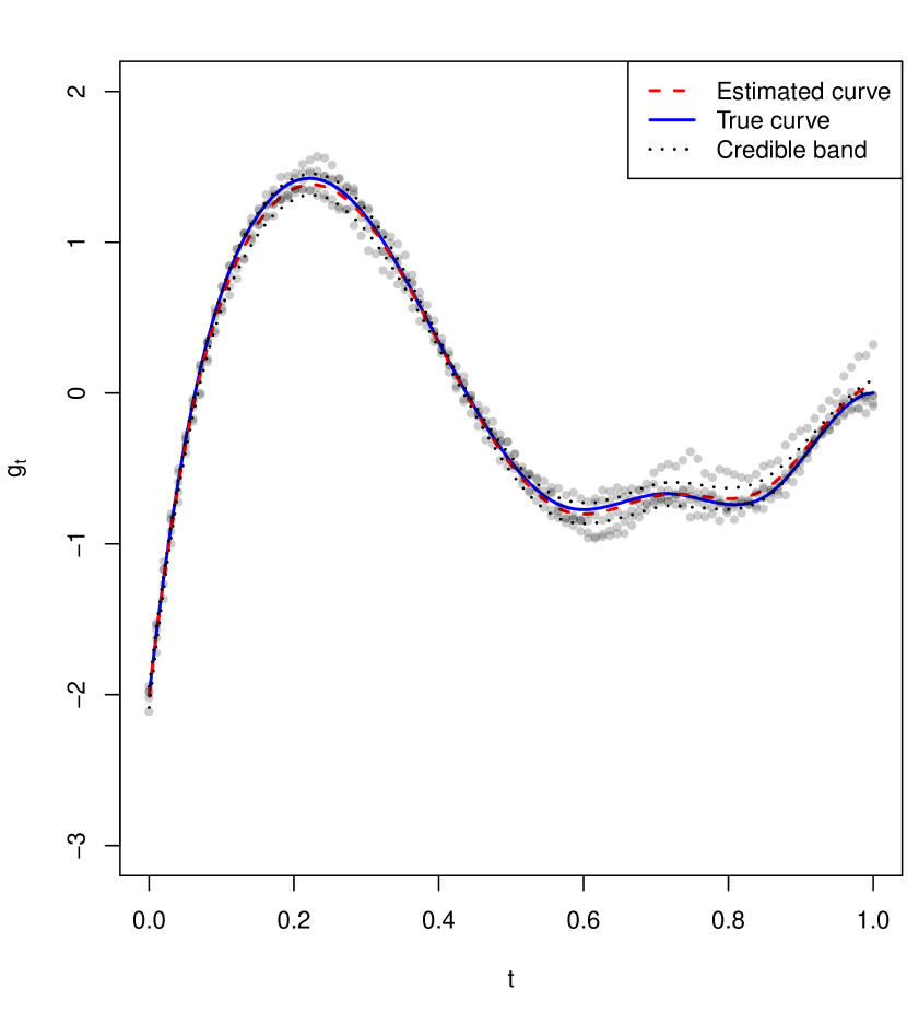
(a) Proposed method ($\sigma=0.1$)

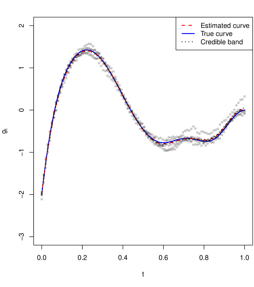
(b) Misspecified correlation structure ($\sigma=0.1$)

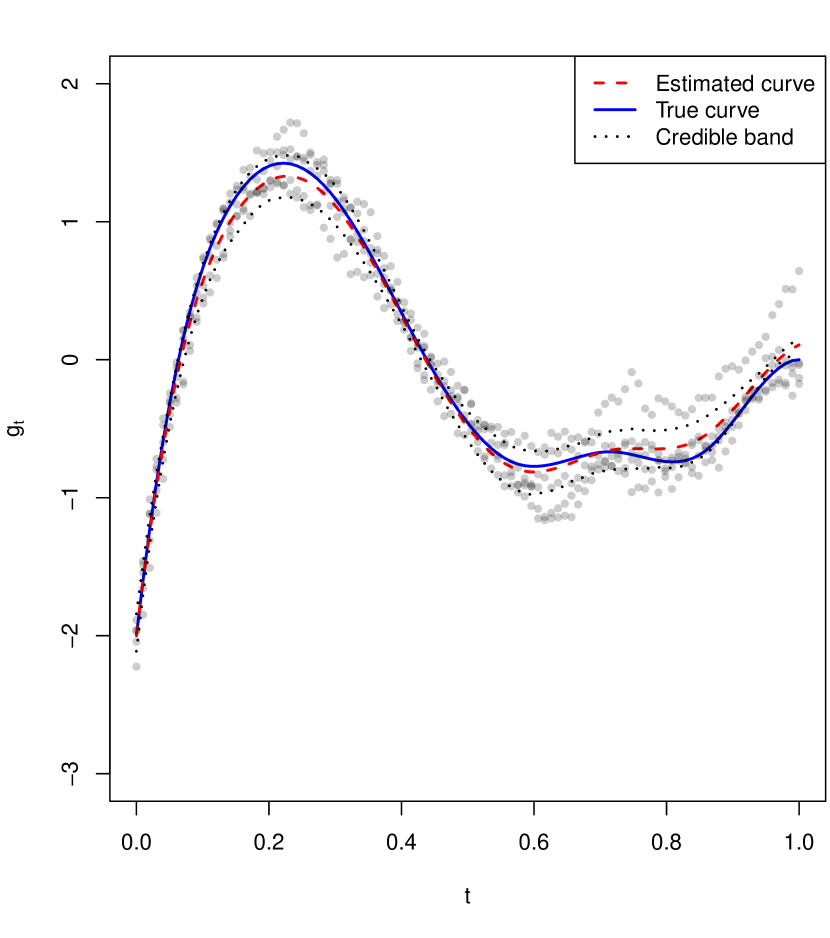
(c) Proposed method ($\sigma=0.2$)

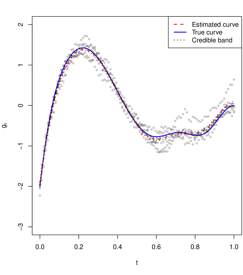
(d) Misspecified correlation structure ($\sigma=0.2$)

Figure 1: Simulated Scenarios 1 and 2. True (blue) and estimated (red) mean curves with a 95% equal-tailed credible band (dashed lines) for one simulated dataset accordingly to the data dispersion, $K=10$ and $w=6$. Figures (a) and (c) refer to our proposed method that estimates the data correlation structure for $\sigma=0.1$ and $\sigma=0.2$ respectively. Figures (b) and (d) were obtained by running VB algorithm assuming independence among observations within a curve for $\sigma=0.1$ and $\sigma=0.2$ respectively.

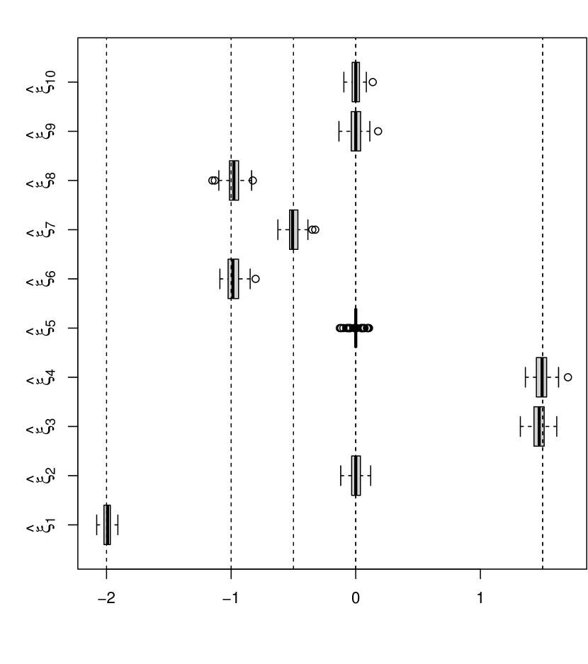
(a) $\sigma=0.1$

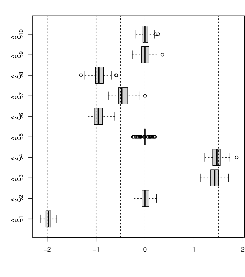
(b) $\sigma=0.2$

Figure 2: Simulated Scenarios 1 and 2. Boxplots of the estimates of the basis function coefficients, $\hat{\xi}_{k}s$, generated from 100 simulated datasets accordingly to the data dispersion, $K=10$ and $w=6$. The dashed lines correspond to the true values of the basis coefficients.

3.2 Simulated Scenario 3

For simulation Scenario 3, we evaluate our method’s performance when we have periodic data. We adapt the second simulated study from Sousa et al., (2024) to include within-curve correlation by assuming a correlation decay parameter $w=6$ in $\Psi(\cdot)$. The data is generated as a linear combination of trigonometric functions with a noise variance of $\sigma^{2}=0.1^{2}$ and same evaluation points $t_{ij}=t_{j}\in[0,2\pi]\;\forall i=1,\dots,5$.

The curves are generated as follows:

$$y(t_{ij})=\cos(t_{ij})+\sin(2t_{ij})+\varepsilon(t_{ij}),$$ (44)

with $\varepsilon(t_{ij})\sim GP(0,\sigma^{2}\Psi(.))$.

For periodic data, Fourier basis functions are typically used to represent the data. Given the simplicity of the generated curves, we employ ten Fourier basis functions. Similar to previous scenarios, Table 2 presents the mean estimated basis coefficients as the simple average across the five curves and simulated datasets. Figure 3(a) shows the boxplots of $\hat{\xi}_{k}$ across all simulated datasets. Notably, only two basis functions showed non-zero values, indicating that these basis functions sufficiently represent the data. Table 2 also includes the standard deviations of the average estimated basis coefficients, demonstrating high precision in the estimates.

To illustrate the fidelity of the estimated curve, Figure 3(b) shows the estimated mean curve in one simulated dataset, along with a $95\%$ equal-tailed credible band calculated as the average of the results obtained from the five curves. The estimated mean curve closely align with the true one, with narrow credible band. Additionally, our method satisfactorily estimated the correlation decay parameter, averaging $6.5603$ across the 100 simulated datasets.

Table 2: Simulated Scenario 3. Mean estimates for the basis function coefficients (Mean) over the 100 simulated datasets when $\sigma=0.1$, $K=10$, and $w=6$. The mean estimates are computed as $\frac{1}{100}\sum_{s=1}^{100}\hat{\xi}_{k}^{s}$, where $\hat{\xi}_{k}^{s}=\frac{1}{m}\sum_{i=1}^{M}\hat{\xi}_{ki}^{s}$ as described in Section 3. We also display their respective standard deviations (SD).

	Mean	SD
$\xi_{1}$	$0.0026$	$0.0169$
$\xi_{2}$	$1.7678$	$0.0243$
$\xi_{3}$	$1.7700$	$0.0242$
$\xi_{4}$	$0.0008$	$0.0138$
$\xi_{5}$	$0.0016$	$0.0123$
$\xi_{6}$	$0.0009$	$0.0137$
$\xi_{7}$	$0.0037$	$0.0170$
$\xi_{8}$	$-0.0008$	$0.0132$
$\xi_{9}$	$-0.0001$	$0.0150$
$\xi_{10}$	$0.0011$	$0.0123$

(a)

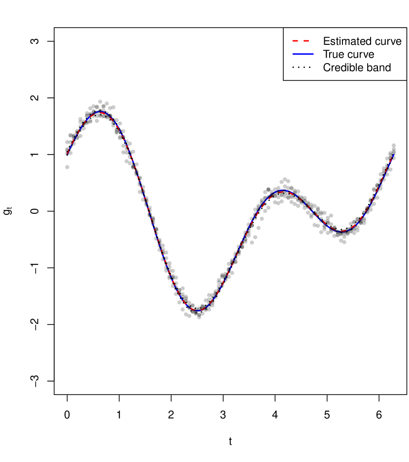
(b)

Figure 3: Simulated Scenario 3. Figure (a) shows the boxplots of basis coefficients estimates, $\hat{\xi}_{k}s$, generated from 100 simulated datasets when $\sigma=0.1$, $K=10$, and $w=6$. The dashed line at zero was added to show which basis functions are being removed when representing the functional data. Figure (b) displays true (blue) and estimated (red) mean curves with a 95% equal-tailed credible band (dashed lines) for one simulated dataset when $\sigma=0.1$, $K=10$, and $w=6$

4 Real Data Analysis

In this section, we apply our proposed method to the well-known motorcycle dataset available in the faraway R Package. This dataset has been extensively analyzed in the literature (Silverman,, 1985; Eilers and Marx,, 1996; Curtis B. Storlie and Reich,, 2010; Schiegg et al.,, 2012; de Souza and Heckman,, 2014). It consists of 133 measurements of head acceleration (in units of g) taken over time during a simulated motorcycle accident. We jittered the time points by adding a small random noise to them, because some time points have multiple acceleration measurements, which impedes the use of smoothing methods.

We applied our proposed method to represent the motorcycle data using 20 cubic B-splines basis functions ($K=20$). To initialize the scale parameter $\delta_{2}^{*}$ of the variational distribution of the noise variance $\sigma^{2}$ in our algorithm, we consider the mean square error from a regression spline with 20 basis functions. Specifically, $\delta_{2}^{*}$ is set so that the initial mean of the variational distribution of $\sigma^{2}$ matches the mean square error obtained from the fitted B-splines, with a sufficiently large variance. We set the correlation decay parameter $w=10$ and $\lambda_{2}^{*}=100$. For the inverse-gamma prior distribution of $\sigma^{2}$, we consider a large prior mean (e.g., 30) and a large prior variance (e.g., 10). For the inverse-gamma prior distribution of $\tau^{2}$, we consider a non-informative prior. As in the simulated studies, we initially include all basis functions in the data representation. The ELBO convergence threshold was set to 0.001.

We compare our proposed method with three commonly used approaches for smoothing functional data. Unlike our method, these alternative approaches cannot fit multiple curves simultaneously. However, because the motorcycle data is represented as a single curve, we can compare the performance of our approach with regression splines, LASSO (Tibshirani,, 1996), and Bayesian LASSO (Park and Casella,, 2008). For all methods, we use the same number and set of basis functions. In the cases of the Bayesian Lasso and Lasso, we utilize the matrix of basis functions as the input for the design matrix.

Furthermore, for LASSO, we consider a grid of values defined by the R function seq(0.001, 1, length = 9) to determine the smoothing parameter. The parameter that yielded the best performance was then used for comparison with the other methods.

The methods are compared based on the adjusted $R^{2}$ and by visually inspecting the smoothed data. Table 3 presents the adjusted $R^{2}$ values obtained from all methods. Our proposed method exhibited the best performance with the highest adjusted $R^{2}$, while the Bayesian LASSO had the worst performance. Notably, our method was the only one that reduced the number of basis functions used to fit the data, using only seven out of the 20 basis functions. In contrast, the Bayesian LASSO and LASSO methods, which also incorporate regularization and are capable of performing basis function selection utilized all 20 basis functions. Additionally, LASSO and regression splines had similar performances in terms of adjusted $R^{2}$.

Figure 4 shows the mean curves estimated by the three methods with a $95\%$ credible band for our proposed method. Visually, the estimated curves obtained from our proposed method, regression splines and LASSO closely align in some regions. Additionally, we note that the Bayesian LASSO penalizes some regions more heavily than the other methods. For example, in the 18-23 ms range, the Bayesian LASSO estimates higher head acceleration than the other methods, and in the 27-32 ms range, it estimates lower head acceleration than the other methods.

Notably, our proposed method not only selects the number of basis functions but also identifies which specific basis functions are preferable for representing the data along the range of evaluation points. In our application to the motorcycle data, we found that only seven out of the 20 basis functions should be used, specifically the basis functions in columns six to 12 in the B-splines matrix. Additionally, our method was the only one to capture the expected behavior present in the data. Specifically, since the data measures head acceleration in a simulated motorcycle accident, it is expected that head acceleration should be zero at the start of the experiment, as the impact has not yet occurred. Similarly, after the impact, head acceleration should return to zero. Our method was the only one to capture this expected behavior.

Despite the estimated within-curve correlation being negligible ($\hat{w}=10^{6}$), indicating minimal or no correlation in the head measurements, our proposed method remains highly effective. It demonstrates comparable, if not superior, performance to commonly used techniques in functional data representation. This highlights how adaptable and reliable our method is, making it a compelling choice even when within-curve correlation is not significant.

Table 3: Real Data Analysis. Comparative table of adjusted $R^{2}$ values obtained from our proposed method, regression splines, Bayesian LASSO and LASSO with K = 20 and same set of basis functions.

Method	Adjusted $R^{2}$
Proposed method	$0.7891$
Regression splines	$0.7722$
Bayesian LASSO	$0.7457$
LASSO	$0.7715$

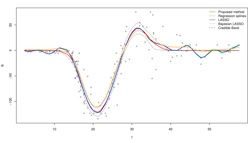
Figure 4: Real Data Analysis. Time in ms in the x axis and head acceleration in units of g in the y axis. Estimated mean curves using our proposed method (red), regression splines (green), LASSO (blue) and Bayesian LASSO (orange), with a 95% equal-tailed credible band (dashed lines) for the motorcycle dataset.

5 Discussion

In this work, we extend the approach proposed in (Sousa et al.,, 2024) to select basis functions for functional data representation in two ways: (i) by accounting for within-curve correlation and (ii) by utilizing VB instead of a Gibbs sampler. Our proposed method accurately selects the correct set of basis functions from a candidate set while incorporating within-curve correlation. Simulation studies demonstrate that our method effectively identifies the true underlying structure of the data across various scenarios. Additionally, our approach is applicable to different types of functional data, as evidenced by the satisfactory results obtained in the simulated studies using both B-splines and Fourier basis functions. Our variational EM algorithm not only recovers the basis coefficients and the correct set of basis functions but also estimates the existing within-curve correlation. Although our method does not quantify the uncertainty in the estimation of the correlation decay parameter, it effectively improves the measurement of uncertainty in basis function selection.

Our application to the motorcycle dataset further showcased the practical utility of our proposed method. Compared to other techniques such as regression splines, LASSO and Bayesian LASSO, our method not only achieved comparable or superior performance in terms of adjusted $R^{2}$ but also offered the advantage of selecting a more parsimonious set of basis functions. Additionally, our Bayesian approach allows for the measurement of uncertainty through the construction of credible bands, which the other methods do not provide.

Additionally, we investigate the computational efficiency of a VB approach compared to a Gibbs sampler in performing basis selection through simulation studies. For this comparison, we assume independence among observations within a curve. The detailed results are provided in the supplementary material. Notably, our VB method demonstrated similar performance to the Gibbs sampler while using only thousandths of the computational time required by the Gibbs sampler. This highlights that variational inference methods provide an effective alternative for computing the posterior distribution, offering significant reductions in computational cost.

For future work, the within-curve correlation structure considered in this study can be extended to assume that both correlation and variance of the errors are functional. This would provide a more flexible dependence structure and improve the model’s adaptability.

References

- Bishop, (2006) Bishop, C. M. (2006). Pattern recognition and machine learning. Springer google schola, 2:1122–1128.
- Blei et al., (2017) Blei, D. M., Kucukelbir, A., and McAuliffe, J. D. (2017). Variational inference: A review for statisticians. Journal of the American statistical Association, 112(518):859–877.
- Crainiceanu et al., (2009) Crainiceanu, C. M., Staicu, A.-M., and Di, C.-Z. (2009). Generalized multilevel functional regression. Journal of the American Statistical Association, 104(488):1550–1561.
- Curtis B. Storlie and Reich, (2010) Curtis B. Storlie, H. D. B. and Reich, B. J. (2010). A locally adaptive penalty for estimation of functions with varying roughness. Journal of Computational and Graphical Statistics, 19(3):569–589.
- de Souza and Heckman, (2014) de Souza, C. P. E. and Heckman, N. E. (2014). Switching nonparametric regression models. Journal of Nonparametric Statistics, 26(4):617–637.
- Dias et al., (2013) Dias, R., Garcia, N. L., and Schmidt, A. M. (2013). A hierarchical model for aggregated functional data. Technometrics, 55(3):321–334.
- Earls and Hooker, (2017) Earls, C. and Hooker, G. (2017). Variational Bayes for Functional Data Registration, Smoothing, and Prediction. Bayesian Analysis, 12(2):557 – 582.
- Eilers and Marx, (1996) Eilers, P. H. C. and Marx, B. D. (1996). Flexible smoothing with B-splines and penalties. Statistical Science, 11(2):89 – 121.
- Goldsmith et al., (2011) Goldsmith, J., Wand, M. P., and Crainiceanu, C. (2011). Functional regression via variational bayes. Electronic journal of statistics, 5:572.
- Huo et al., (2023) Huo, S., Morris, J. S., and Zhu, H. (2023). Ultra-fast approximate inference using variational functional mixed models. Journal of Computational and Graphical Statistics, 32(2):353–365.
- Ishwaran and Rao, (2005) Ishwaran, H. and Rao, J. S. (2005). Spike and slab variable selection: Frequentist and bayesian strategies. The Annals of Statistics, 33(2):730–773.
- Jordan et al., (1999) Jordan, M. I., Ghahramani, Z., Jaakkola, T. S., and Saul, L. K. (1999). An introduction to variational methods for graphical models. Machine learning, 37:183–233.
- Kuo and Mallick, (1998) Kuo, L. and Mallick, B. (1998). Variable selection for regression models. Sankhyā: The Indian Journal of Statistics, Series B, pages 65–81.
- Li and Ma, (2023) Li, T. and Ma, J. (2023). Dirichlet process mixture of gaussian process functional regressions and its variational em algorithm. Pattern Recognition, 134:109129.
- Liu et al., (2019) Liu, C., Li, H.-C., Fu, K., Zhang, F., Datcu, M., and Emery, W. J. (2019). Bayesian estimation of generalized gamma mixture model based on variational em algorithm. Pattern Recognition, 87:269–284.
- Park and Casella, (2008) Park, T. and Casella, G. (2008). The bayesian lasso. Journal of the american statistical association, 103(482):681–686.
- Ramsay and Silverman, (2005) Ramsay, J. O. and Silverman, B. W. (2005). Functional Data Analysis. Springer.
- Schiegg et al., (2012) Schiegg, M., Neumann, M., and Kersting, K. (2012). Markov logic mixtures of gaussian processes: Towards machines reading regression data. In Artificial Intelligence and Statistics, pages 1002–1011. PMLR.
- Silverman, (1985) Silverman, B. W. (1985). Some aspects of the spline smoothing approach to non-parametric regression curve fitting. Journal of the Royal Statistical Society. Series B (Methodological), 47(1):1–52.
- Sousa et al., (2024) Sousa, P. H. T., de Souza, C. P., and Dias, R. (2024). Bayesian adaptive selection of basis functions for functional data representation. Journal of Applied Statistics, 51(5):958–992.
- Tibshirani, (1996) Tibshirani, R. (1996). Regression shrinkage and selection via the lasso. Journal of the Royal Statistical Society Series B: Statistical Methodology, 58(1):267–288.
- Wainwright et al., (2008) Wainwright, M. J., Jordan, M. I., et al. (2008). Graphical models, exponential families, and variational inference. Foundations and Trends® in Machine Learning, 1(1–2):1–305.
- Williams and Rasmussen, (2006) Williams, C. K. and Rasmussen, C. E. (2006). Gaussian processes for machine learning, volume 2. MIT press Cambridge, MA.
- Xian et al., (2024) Xian, C., de Souza, C. P., Jewell, J., and Dias, R. (2024). Clustering functional data via variational inference. Advances in Data Analysis and Classification, pages 1–50.