First Tree-like Quantum Data Structure: Quantum B+ Tree
Abstract.
Quantum computing is a popular topic in computer science, which has recently attracted many studies in various areas such as machine learning, network and cryptography. However, the topic of quantum data structures seems long neglected. There is an open problem in the database area: Can we make an improvement on existing data structures by quantum techniques? Consider a dataset of key-record pairs. Given an interval as a query range, a B+ tree can report all the records with keys within this interval, which is called a range query. A classical B+ tree answers a range query in time, where is the total number of records and the output size is the number of records in the interval. It is asymptotically optimal in a classical computer but not efficient enough in a quantum computer, because it is expected that the execution time and the output size are linear in a quantum computer.
In this paper, we propose the quantum range query problem. Different from the classical range queries, a quantum range query returns the range query results in quantum bits, which has broad potential applications due to the foreseeable future advance of quantum computers and quantum algorithms. To the best of our knowledge, we design the first tree-like quantum data structure called the quantum B+ tree. Based on this data structure, we propose a hybrid quantum-classical algorithm to do the range search. It answers a static quantum range query in time, which is asymptotically optimal in quantum computers. Since the execution time does not depend on the output size (i.e., , which could be as large as ), it is significantly faster than the classical data structure. Moreover, we extend our quantum B+ tree to answer the dynamic and -dimensional quantum range queries efficiently in and time, respectively. Our experimental results show that our proposed quantum data structures achieve up to 1000x improvement in the number of memory accesses compared to their classical competitors.
1. Introduction
Consider a dataset where each item in this dataset is in the form of a key-record pair. The range query problem, which is to report all the items with keys within a given query range, has been a longstanding problem extensively studied and applied in broad applications. For example, a teacher may need to list all the students who obtained 40-60 marks in an exam, a smartphone buyer may need to list all the smartphones that sit around $200-$400, and a traveler may want to list all the nearby spots. Apart from directly returning all the results to the user, range queries have also been applied as a subroutine of many problems in various areas. One typical example is the recommendation systems (gupta2013location; covington2016deep), where range queries are commonly performed to extract a relatively small set of candidates first from the entire dataset as per user’s request and then a recommendation algorithm is executed to find the top recommendations from the candidates.
Consider a movie dataset containing a list of movies each described as a key-record pair where the key is the release date and the record is a feature vector which represents some attributes such as name, genre and cast. Assume that Alice wants to find an interesting movie of 1990s. We first perform a range query of finding a candidate set of all the movies with release date from 1990 to 1999 and then give recommendations based on .
To answer range queries, many data structures (bayer2002organization; comer1979ubiquitous; o1996log) have been proposed in classical computers to store the key-record pairs. One representative and widely-used data structure is the B+ tree (comer1979ubiquitous). It answers a range query in time, where is the total number of key-record pairs and the output size is the number of records in the query range. Based on (yao1981should), the B+ tree is asymptotically optimal for range queries in classical computers. Note that for all range queries, the linear time of generating all the results is inevitable, which is not efficient enough when range queries are used as subroutines of algorithms in quantum computers.
Recently, quantum algorithms have attracted a lot of attention. Many quantum algorithms (shor1994algorithms; grover1996fast; ruan2017quantum; adhikary2020supervised; li2021vsql; kerenidis2017quantum) have been proposed and are expected to show quadratic or even exponential speedup compared to classical algorithms, and thus many linear-complexity problems can be solved in sub-linear time in quantum computers. For instance, a recent quantum recommendation system (kerenidis2017quantum) shows poly-logarithm time complexity to the input size. However, when we consider the scenario where the recommendation is made among the candidates in a user-specified query range, the potential of quantum algorithms is limited since all the efficiency of the sublinear-time quantum algorithms is ruined by the linear time of generating all the candidates of traditional range queries.
Motivated by the critical limitations of the classical range query in quantum computers, we propose the problem called the quantum range query, which returns the answer in quantum bits, since we notice that quantum algorithms normally have the input in the form of quantum bits. Specifically, the quantum range query does not return a list of key-record pairs, but returns the quantum bits in a superposition of all the key-record pairs with keys within the query range , where the superposition is the ability of a quantum system to be in multiple states simultaneously. For example, consider a movie dataset , where is the number of movies and each movie is represented as a key-record pair as mentioned above. Assume that we can construct a data structure in the quantum computer to store all the key-record pairs. If Alice wants to obtain all the movies of the 1990s, a quantum range query will search on the data structure and return the quantum bits in a superposition of all the movies whose is within the interval . Motivated by the different scenarios in real-world applications, we study the quantum range query problems in three different cases. The first case is that the dataset is immutable, so the problem is called the static quantum range query. The second case is that insertions and deletions are supported in the dataset, and the problem is called the dynamic quantum range query. The third case is that the keys in key-record pairs are multi-dimensional points (e.g., the locations of restaurants), so the problem is called the multi-dimensional quantum range query.
The quantum range queries have many potential applications. (1) In relational database queries, it is common to have a numerical query range as a query condition (e.g., finding the movie with the highest ranking for release date between 1990 and 1999). To execute such query, a range query is commonly considered for query optimization. Specifically, a range query of retrieving all movies released between 1990 and 1999 is first performed to narrow down the search space to a small subset, and then finding the highest ranking movie could be executed efficiently on the subset. In the literature, some quantum algorithms have been proposed to support efficient database queries such as finding the database record that has the highest value on a certain field. When enabling query optimization, if we use a quantum range query to obtain the narrowed search space, the result of the quantum range query (in quantum bits) could be applied in those quantum algorithms for fast database queries. (2) In a quantum recommendation system as we mentioned previously, a range query is first used as a filter to find a small set of candidates from the entire dataset, and then a quantum recommendation algorithm (kerenidis2017quantum) is used to make the top recommendation from the candidates. A quantum range query, instead, returns a superposition of the candidates which can be directly applied to these existing quantum recommendation algorithms. (3) Data binning (dougherty1995supervised) is a popular approach to improve the accuracy of various machine learning algorithms (berg2021deep; xue2017efficient), which applies range queries to group similar items within a query range (i.e., a data bin) together. Since it is foreseeable that similar quantum machine learning algorithms (adhikary2020supervised) could also benefit from data binning, the quantum range queries give the quantum binning results where the items in each bin are output in the form of a superposition that can be readily used in quantum machine learning algorithms. (4) Campos et.al. (campos2010simple) studied how to use KNN to do movie recommendations. They found that it can improve the accuracy to only consider the rating datasets from the last month before the recommendation time in different years. That means they need to select the records produced in the same month but in different years. Given a B+ tree containing all the movies sorted by the dates in the year, the calculation costs time since the range query returns records on average. Assume that we can use a quantum range query to select the records in time. Note that there is an existing quantum KNN algorithm (ruan2017quantum) where is the dimension of the feature vector. Therefore, the whole process only costs . In most cases, is much smaller than . Assuming , we can find that the quantum time-periodic-biased KNN is exponentially faster than its classical competitor.
Besides the above applications, we expect that it will be common for quantum algorithms to have the input and output in the form of superpositions. For example, the HHL algorithm (harrow2009quantum) returns the answer to a linear system of equations in a superposition, and it becomes a subroutine of the quantum SVM (rebentrost2014quantum). Therefore, we believe that in the future, more quantum algorithms will benefit from the quantum range queries which return the query results in superpositions. In the database area, we expect the emergence of more quantum database search algorithms (e.g., the quantum top- query), which could leverage the quantum data structures for query optimization (e.g., applying the quantum range query to narrow down the searching space).
The quantum range query problem has two distinctive characteristics. The first characteristic is that it allows the utilization of data structures, which corresponds to building an index to accelerate the database queries that has been a common approach in the database area. Existing quantum algorithms (grover1996fast; boyer1998tight; grover2005partial; durr1996quantum) do not consider a data structure and only focus on searching with unstructured data, and thus they cannot solve the quantum range query problem efficiently. Among them, the best quantum range query algorithm adapted from (boyer1998tight) returns the result of items in time, which is inefficient when the dataset size grows large.
The second characteristic is the use of quantum computation to handle superpositions efficiently. As mentioned previously, the time complexity for a range query in classical computer is already asymptotically optimal, where the cost of listing out all the results has no chance to be improved. In the quantum range query problem, however, since we aim to obtain the results in the form of a superposition, it is possible to eliminate this cost and thus achieve a better time complexity with the techniques in quantum computation.
Motivated by this, we propose the quantum B+ tree, which is the first tree-like quantum data structure to the best of our knowledge. Since the B+ tree (comer1979ubiquitous) is one of the most fundamental and widely-used data structures, we believe that it is suitable to start a new world of quantum data structures with the B+ tree. We design our quantum B+ tree with two components, the classical component and the quantum component. The classical component follows the classical B+ tree, which allows us to leverage its effective balanced tree structure. The quantum component stores a concise “replication” of the hierarchical relationships in the B+ tree in the quantum memory, which could load the relationships in the form of superpositions efficiently in quantum computers due to quantum parallelism.
Empowered by the two-component design of our quantum B+ tree, we propose a hybrid quantum-classical algorithm called the Global-Classical Local-Quantum (GCLQ) search to solve the quantum range query problem. It involves two main steps. The first step is called the global classical search, which finds a very small number (i.e., at most two) of candidate nodes from the classical B+ tree. It is guaranteed that all the relevant results are covered in the candidate nodes and account for a significant amount under the candidate nodes (i.e., at least of the items under candidate nodes are the relevant results). Meanwhile, the global classical search is very efficient owing to the effective structure of B+ tree. The second step is called the local quantum search, which returns a superposition of all the exact query results from the candidate nodes with efficient quantum parallelism techniques in the quantum memory. As a result, the time complexity of our proposed GCLQ search is , which is asymptotically optimal in quantum computers. This improves the optimal classical result by reducing the cost and is much more efficient than the time complexity of the existing quantum algorithms without using any data structure.
We also propose two extensions of our quantum B+ tree to solve the dynamic quantum range query and the multi-dimensional quantum range query. Our two-component design with a classical B+ tree structure retained as a “prototype” allows us to flexibly extend our quantum B+ tree to the B+ tree variants in classical computers. As such, we extend our quantum B+ tree to the dynamic quantum B+ tree by adapting the logarithmic method (bentley1980decomposable), which supports inserting a new item into the tree and deleting an existing item from the tree. All the insertions and deletions are also replicated to the quantum component of the tree, which is efficient due to the conciseness of the quantum component. We show that each insertion and deletion can be done in time, and the dynamic range query can be done in with the dynamic quantum B+ tree. To handle the multi-dimensional quantum range query, we also propose the quantum range tree based on the classical range tree (bentley1978decomposable) (which handles a classical -dimensional range query in time). This is similar to the mechanism of constructing the quantum B+ tree from a classical B+ tree. The multi-dimensional quantum range query can be answered in time, which also improves the classical time complexity by the cost.
Therefore, we first propose the static quantum B+ tree, which is the first tree-like quantum data structure to our best knowledge. We choose the B+ tree (comer1979ubiquitous) as the first data structure to study in quantum computers. Since the B+ tree is the most fundamental and widely-used data structure, it is considered the most suitable one to open a new world of quantum data structures. To take the full advantages of quantum parallelism, we design a hybrid quantum-classical algorithm to answer the static quantum range query. The hybrid design is very popular, especially in quantum machine learning (kim2001batch). According to (abohashima2020classification), many studies such as (adhikary2020supervised; chakraborty2020hybrid; benedetti2019generative; schuld2019quantum; schuld2020circuit; ruan2017quantum; mitarai2018quantum) used hybrid quantum-classical algorithms to do machine learning, since this design can reduce the circuit depth (which signifies the total number of instructions in the quantum algorithm) so that high performance can be obtained. Specifically, the same B+ tree is stored both in a quantum computer and a classical computer. The classical component of the tree-building algorithm will bulk load the data and construct the B+ tree in a manner like (kim2001batch). We formally define the concept of a quantum memory in Section 3, which is used to store mappings between bit-strings in a quantum computer. Each modification of the B+ tree in the classical computer will reflect in the quantum memory correspondingly. For example, if we add an edge from Node 2 to Node 3 in the B+ tree in the classical computer, we also add a mapping from 2 to 3 in the quantum memory. In the quantum computer, all the mappings from the nodes in the upper level to nodes in the lower level are maintained in the quantum memory. Our proposed quantum range query algorithm has the following two main steps.
In summary, our contributions are shown as follows.
-
•
We are the first to study the quantum range query problems.
-
•
We are the first to propose a tree-like quantum data structure, which is the quantum B+ tree.
-
•
We design a hybrid quantum-classical algorithm that can answer a quantum range query on a quantum B+ tree in time, which does not depend on the output size and is asymptotically optimal in quantum computers.
-
•
We further extend the quantum B+ tree to the dynamic quantum B+ tree that supports insertions and deletions in time, and the complexity of the quantum range query on the dynamic quantum B+ tree is .
-
•
We also extend the quantum B+ tree to the quantum range tree, which answers a -dimensional quantum range query in time.
-
•
We conducted experiments to confirm the exponential speedup of the quantum range queries on real-world datasets. We considered both the time-based range query and the location-based range query, which are widely used in real-world applications. In our experiments, our quantum data structure is up to faster than the classical data structure.
The rest of the paper is organized as follows. In Section 2, we first introduce some basic knowledge used in this paper about quantum algorithms. We formally define the quantum range query problems in Section 3. In Section 4, we show the design of the quantum B+ tree and introduce our algorithm to answer the quantum range query. In Section 5, we extend the quantum B+ tree to the dynamic and multi-dimensional versions. Section 6 presents our experimental studies. In Sections 7 and 8, we introduce the related work and conclude our paper, respectively.
2. Preliminaries
A bit is a basic unit when we store data in the memory or on disks. In classical computers, a bit has two states (i.e., 0 and 1). A bit in quantum computers is known as a quantum bit, which is called a qubit in this paper for simplicity. Similar to a bit in classical computers, a qubit also has states. Following (dirac1939new; bayer2002organization), we introduce the “Dirac” notation (i.e., “”) to describe the states of a qubit. Specifically, we write an integer in (e.g., ) to describe a basis state, and we write a symbol in (e.g., ) to describe a mixed state (more formally known as a superposition). Note that the symbol in a superposition of a qubit is used to denote this qubit. That is, we say that the qubit has the superposition .
We have two basis states of a qubit, and , which correspond to state 0 and state 1 of a classical bit, respectively. Different from a classical bit, a qubit could have a state “between” and , which is described by a superposition . Specifically, superposition is represented as a linear combination of the two basis states: , where and are two complex numbers called the amplitudes and we have ( denotes the absolute square of a complex number ). In quantum computers, instead of directly obtaining the value of a bit, we measure a qubit , which will “collapse” its superposition and obtain the result state 0 with probability or state 1 with probability (note that the sum of the probabilities is equal to 1). For instance, let be a qubit with superposition . If we measure , we can obtain 0 with probability or 1 with probability .
Similar to a register in a classical computer, we define a quantum register to be a collection of qubits. Consider a quantum register with two qubits. The basis states of the two qubits will contain all the combinations of the basis states of single qubits, i.e., , , and . If we measure one of the qubits, this measurement may change the state of the other qubit. Such phenomenon is widely known as quantum entanglement (schrodinger1935discussion).
Consider the following example. For simple illustration, all the amplitudes in this example only have real parts (of complex numbers). Let be a quantum register with two qubits and , where the measurement of will change the state of . Specifically, , which is measured to be 0 or 1 with probability both equal to . If 0 is obtained, the state of will be changed to , and otherwise, it will be changed to . As such, the state of (i.e., ) can be represented as
It indicates that the two entangled qubits have 4 basis states , , and with amplitudes , , and , respectively. It can be verified that the sum of the absolute squares of all the 4 amplitudes is still equal to 1. We can extend this system to a quantum register with qubits which have basis states and the corresponding amplitudes.
The states of qubits can be transformed by quantum gates in a quantum circuit, which work similarly as the gates and circuits in classical computers. We can also measure a qubit in a quantum circuit. In the following, we introduce three common types of quantum gates that will be used in this paper, namely a Hadamard gate, an -gate and a controlled- gate. A Hadamard gate (hadamard1893resolution; nielsen2001quantum) transforms into and transforms into . An -gate (nielsen2001quantum) swaps the amplitudes of and . A controlled- gate has two parts, the control qubit, says , and the target qubit, says . A controlled- gate applies an -gate on the target qubit if the control qubit is , and otherwise, it keeps the target qubit unchanged.
For example, assume an input . After being transformed by a Hadamard gate, we have . Clearly, if we now measure , we will always obtain 0. We give more examples about the -gate and the controlled- gate shortly.
A quantum circuit could involve the combination of multiple input qubits and multiple gates. Since the state transformations and measurements for each qubit follow the timeline of a wire, we could describe the state changes in an ordered list of events. For example, we are given a quantum circuit with two input qubits and that is described as follows.
-
(1)
Apply an -gate on .
-
(2)
Apply a controlled- gate where the control qubit is and the target qubit is .
Consider the following three examples of input:
-
(1)
. After the -gate on , . Since , we apply an -gate on , and thus the result is .
-
(2)
. After the -gate on , . Since , we do nothing, and thus the result is .
-
(3)
. After the -gate on , . The result is .
Following prior studies (grover1996fast; shor1994algorithms; wiebe2015quantum; zhang2018quantum), we call such a quantum transformation consisting of a series of quantum gates in a quantum circuit as a quantum oracle. A quantum oracle can be regarded as a black box of a quantum circuit where we only focus on the quantum operation it can perform but skip the detailed circuit. Since different gate sets (which correspond to the instruction sets in classical computers) may cause different time complexities and the general quantum computer is still at a very early stage, we normally use the query complexity to study quantum algorithms, which is to measure the number of queries to the quantum oracles. In the quantum algorithm area, many studies (li2021sublinear; kapralov2020fast; montanaro2017quantum; naya2020optimal; hosoyamada2018quantum; li2019sublinear; kieferova2021quantum) assume that a quantum oracle costs time, and analyze the time complexity based on this assumption. We thus follow this common assumption in this paper.
3. Problem Definition
In this section, we formally define the quantum range query problems in the static, dynamic and multi-dimensional cases, respectively.
We first consider the static quantum range query problem (for simplicity, it is simply called the quantum range query problem). We are given an immutable dataset of items. Each item in is represented as a key-record pair for . Note that the subscription in represents the index of this pair, and the indices start from 0. Each key is an integer, and each record is a bit-string. Note that in our problem, the keys are integers, but they can be easily extended to float numbers. A range query of lower bound and upper bound is denoted as . In classical range query problem, returns a list of key-record pairs whose keys fall in range . Let be the number of items that returns, and let be the indices of the returned items. The returned list of is thus represented as . In the quantum range query problem, we aim to return a superposition of all the key-record pairs in the list. We formally define the quantum range query problem as follows.
Definition 3.1 (Quantum Range Query).
Given an immutable dataset and two integers and where , a quantum range query is to return the following superposition
such that for each , .
Note that in the quantum range query, we return a superposition which is the linear combination of all the desired key-record pairs. It can be observed that for each , the probability of obtaining is equal to .
Next, we also define the dynamic quantum range query. In the dynamic case, instead of having an immutable dataset, we consider a dynamic dataset that supports the insertion and deletion operations. Specifically, an insertion operation inserts a new item into and returns the new dataset . A deletion operation delete an existing item from and returns the new dataset . The dynamic quantum range query is formally defined as follows.
Definition 3.2 (Dynamic Quantum Range Query).
Given a dataset that supports the insertion and deletion operations and two integers and where , a dynamic quantum range query is to return the following superposition
such that for each , .
Note that the only difference between the dynamic and the static quantum range query is whether the given dataset is dynamic.
Finally, we define the multi-dimensional (static) quantum range query. We are given a dataset of key-record pairs (for ), where each key is in the form of a -dimensional vector of integers, i.e., . A multi-dimensional quantum range query also takes lower bound and upper bound as input, where and are also in the form of -dimensional vectors of integers, i.e., and . The multi-dimensional quantum range query is formalized as follows.
Definition 3.3 (Multi-dimensional Quantum Range Query).
Given an immutable dataset where each is in the form of a -dimensional vector (i.e., ) and two -dimensional vectors and where for each , a multi-dimensional quantum range query is to return the following superposition
where for each and , .
4. Quantum B+ Tree
In this section, we propose the quantum B+ tree to solve the quantum range query problems. To the best of our knowledge, no prior studies explored using a data structure in quantum computers. Compared with performing a quantum algorithm on unstructured dataset, using quantum data structures could answer our quantum range query problems more efficiently. We focus on the static quantum B+ tree in this section, and discuss the dynamic and multi-dimensional variants later in Section 5.
Before introducing the details of the quantum B+ tree, we first introduce the concept of the Quantum Random Access Memory (QRAM) which is used to store the quantum data structure and give query results in superpositions. Like the classical RAM, we have the QRAM in quantum computers to read and write quantum states. Following (kerenidis2017quantum; saeedi2019quantum), we assume the existence of a classical-write quantum-read QRAM. It can store a classical value into a given address, and it can accept a superposition of multiple addresses and returns a superposition of the corresponding values due to quantum parallelism. Formally, we define the QRAM as follows.
Definition 4.1 (Quantum Random Access Memory (QRAM)).
A QRAM is an ideal model which can perform the following store and load operations.
-
•
A store operation denoted by stores value into address , where and are two bit-strings.
-
•
A load operation denoted by
(1) takes a superposition of a number of addresses (i.e., for ) as input and loads a superposition of the values of these addresses into the destination quantum register of initial state where denotes the XOR operation.
In our definition of QRAM, the concept of the store operation is similar to a classical RAM where we store into a memory block at address . For simplicity, we also use to denote the value stored at address . In the load operation, the input of multiple addresses and the output of multiple values are handled in superpositions, which is the major difference from a classical RAM. The result of a load operation is written to a quantum register using the XOR operation (i.e., ). For instance, if we set the initial state of the destination quantum register to be , then the exact values will be loaded as follows.
| (2) |
Although the QRAM is still discussed at the theoretical stage and no existing physical implementation is yet available, researchers believe that with the future advances of quantum computers, the QRAM can be implemented to support the above store and load operation very efficiently in the form of quantum oracles (li2021sublinear; kapralov2020fast; montanaro2017quantum; naya2020optimal; hosoyamada2018quantum; li2019sublinear; kieferova2021quantum).
Note that even with the assumption of QRAMs, the quantum range query is still non-trivial. With the concept of QRAM, we can form the following method of answering the quantum range query problems in two steps using the existing quantum algorithms on the unstructured dataset. In the first step of pre-processing (for loading the dataset), for each key-record pair , we store it into a QRAM using the store operation . Clearly, the total time complexity is . In the second step of data retrieval, we first find all the addresses in that are within the query range, which costs time using the state-of-the-art quantum algorithm (brassard1998quantum; boyer1998tight), and then use the load operation to find the resulting superposition of the corresponding values. Totally, the data retrieval step costs . When grows large, this is even worse than the classical range query algorithms (e.g., using the B+ tree) with time complexity logarithm to .
To solve the quantum range query problems more efficiently with QRAM, we propose our quantum data structure called the quantum B+ tree. The major design of our quantum B+ tree is derived from the basic idea of the classical B+ tree. It is well known that the classical B+ tree utilizes a balanced tree structure, which performs a range query in the dataset of size efficiently with time complexity , where is the return size. In classical computers, this time complexity is shown to be asymptotically optimal. For the quantum range queries in quantum computers, we are also interested in the best possible time complexity. To explore that, we introduce another problem called the membership problem, which, given a query key, decides whether this key exists in the dataset . Existing studies have shown that the time complexity lower bound of solving the membership problem in quantum computers is (ambainis1999better; sen2001lower). Based on that, we present the following lemma to show the time complexity lower bound of solving our quantum range queries. For the sake of space, we give a proof sketch for each lemma or theorem in this paper, and the full proof can be found in our technical report (technical_report).
Lemma 4.2.
The time complexity to answer a quantum range query is .
Consider a quantum range query . It answers whether the key exists in the dataset, which is a membership problem of time complexity by (sen2001lower). Therefore, the time complexity of answering a quantum range query is also .
According to the above lemma, we cannot achieve a better time complexity than for the quantum range query. The goal of our static quantum B+ tree is thus to obtain this asymptotically optimal time complexity . Since the time cost of listing all the returned results cannot be reduced in classical range queries, we consider eliminating this cost in our quantum B+ tree, which is feasible in quantum computers that handle the superpositions due to quantum parallelism.
Based on the above analysis, in the following, we first introduce the details of how we design our quantum B+ tree in Section 4.1, and then, we propose our quantum range search algorithm called the global-classical local-quantum search in Section 4.2.
4.1. Design of Quantum B+ Tree
The design of our quantum B+ tree follows the core idea which focuses on representing the structure of the classical B+ tree in quantum computers. Specifically, the hierarchical relationships and node data are stored into the quantum memory (i.e., QRAM). This is to take advantage of the balanced tree structure of the classical B+ tree, which has a tree height of and thus retains the search efficiency. Also, it can utilize the QRAM to process the tree structure and return the range search results in superpositions efficiently by quantum parallelism.
In the following, we first introduce some basic concepts of the classical B+ tree, which is the prototype of our quantum B+ tree. We consider a weight-balanced B+ tree (arge1996optimal). It is a tree data structure that consists of nodes in two types, the internal nodes and the leaves. Each node has a unique ID in the form of an integer, which is used to represent this node. A user parameter called the branching factor is set to be an integer that is a power of 2 and is at least 4. A leaf contains key-record pairs sorted by the keys in ascending order. An internal node has children, each of which is a leaf or an internal node. Each node is also associated with a routing key, says , which represents a range with lower bound and upper bound , and all the key-record pairs under the internal node with routing key have keys within this range. The children under an internal node have non-overlapping routing keys and are sorted by the lower bound of their routing keys. A node or a key-record pair under a leaf could be empty, which is represented as a special mark called . We assume that appears only in the last positions under a node.
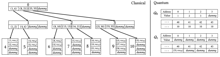
The left part in Figure 1 illustrates an example of the classical component of a classical B+ tree with key-record pairs and the branching factor . It has four internal nodes of ID from 0 to 3 and seven leaves of ID from 4 to 10. For instance, the node of ID 1 (simply called node 1) has routing key (1, 6), indicating that all the data items with keys in range are under node 1. Also, node 1 has four children, two of which are non-dummy leaves and the other two are dummy nodes. For the leave shown as node 4 with routing key (1, 2), two data items (with keys equal to 1 and 2) and two dummy items are assigned.
We define the level of a node to be its distance to the root, where the distance between two nodes is defined to be the minimum number of edges connecting these two nodes. In a B+ tree, all the leaves have the same level. We also define the height of a node to be its distance to a leaf, and the height of the B+ tree is defined to be the height of the root. We define the weight of a node to be the number of all non-dummy key-record pairs under this node. A non-root node of height is said to be balanced if its weight is between and . Further, a non-root node of height is said to be perfectly balanced if its weight is between and .
In our running example shown in the left part of Figure 1, there are 4 non-dummy key-record pairs under node 1 of height equal to 1, and thus the weight of node 1 is equal to 4. This indicates that node 1 is balanced (since 4 is no less than ) but is not perfectly balanced (since 4 is less than ).
A B+ tree is said to be a weight-balanced B+ tree if all its non-root nodes are balanced and its root has at least two non-dummy children. It is easy to verify that the height of a weight-balanced B+ tree with key-records pairs is . Moreover, a weight-balanced B+ tree is said to be perfectly balanced if all its non-dummy nodes are perfectly balanced. It can be verified that the B+ tree shown in the left part of Figure 1 is a weight-balanced B+ tree but is not perfectly balanced.
After introducing the structure of a classical B+ tree, we now discuss how we represent the hierarchical relationships and node data of a B+ tree in QRAM. Since each node contains elements (including dummy), each of which has a child node with a routine key or a key-record pair, we could fit a classical B+ tree into a QRAM storing key-value pairs, where denotes the total number of nodes in the classical B+ tree, a key represents the ID of a tree node and a value stores the related information of this node. This can be done by a traversal of all the tree nodes in any order (in this paper, we choose the breadth-first order for simplicity).
We use two QRAMs, namely the hierarchy QRAM and the data QRAM , to store the hierarchical relationships (i.e., the mapping from each node to its children) and the data (i.e., the routine key of a node or the key-record pair of a leave), respectively. Specifically, we perform store operations on where denotes the total number of nodes in the classical B+ tree as follows. Let (for and ) denote the node ID of the -th child of node in the B+ tree. Specially, if node is a leave with no children, we set . Also, if the -th child of node is , we assign to . Then, for each node and each , we perform a store operation to store value at address , i.e., .
In the right part of Figure 1, we show an example of the quantum B+ tree. In the hierarchy QRAM , totally 44 () addresses are “occupied”. Among them, for instance, node 0 involves storing the IDs of its three non-dummy children (i.e., 1–3) and one into addresses 0–3, respectively, and node 10 involves storing value 10 for all its corresponding addresses 40–43 since it is a leaf.
The data QRAM stores the routine key of each node or the key-record pair of each leave. Similar to , we also perform store operations on . Consider node in the B+ tree. If is an internal node, then for its -th child, we assign the routine key (i.e., a 2-tuple of lower bound and upper bound of this routine key) to a variable, says , which is if the -th child is dummy. If is a leaf, we set to be the -th key-record pair of node or if the -th key-record pair is dummy. As such, for each node and each , we perform a store operation to store pair at address , i.e., .
Continuing our running example in Figure 1, in the data QRAM , we also store values into 44 addresses similarly, where for node 0, since it is an internal node, all values stored are (at addresses 0–3), and for node 10 with two key-record pairs and two dummies, the values at address 40–43 are stored correspondingly.
Note that both QRAMs have data across the same number (i.e., ) of addresses, and at the same address, the value stored are related to the same node or the same key-record pair in a leaf. Thus, it is easy to combine the two QRAMs into one QRAM by using a larger quantum register storing the values of both QRAMs at the same address for implementation. In this paper, for clear structuring and illustration, we use two QRAMs to separate them.
For both and , we could easily retrieve multiple values for the relationships in the tree with one load operation on QRAM. Specifically, in the node QRAM , we perform the following load operation for node ()
| (3) |
where denotes the number of non-dummy children among all the children of node . This operation loads the IDs of all the children of node into a superposition in time. Similarly, on , we can load the key-record pairs under a leaf (with node ID ) with the following load operation
| (4) |
4.2. Global-Local Quantum Range Search
In this section, we propose an algorithm called the global-local quantum range search to solve the quantum range query with our quantum B+ tree.
Recall that our quantum range query aims to return a superposition of all the key-record pairs such that each key in the result is within a query range . To better present our algorithm, we first propose a technique called post-selection which can answer the quantum range query with our dataset stored in a QRAM even in an unstructured way (i.e., without using the quantum B+ tree).
The major idea of post-selection is based on the efficient processing of superpositions of QRAM and the quantum oracle. Specifically, we first apply the store operations to store all the key-record pairs in the dataset in a QRAM, says , which is a pre-processing step. That is, for each , we do a store operation . We can thus obtain a superposition of all the key-record pairs as by a load operation on in time. After obtaining this superposition, we design a quantum oracle as follows to post-select the superposition of the desired items within the query range .
Let denote the set of indices of all the key-record pairs in the dataset such that the keys are within , and let denote the set of all the remaining indices. First, we place an additional qubit with initial state in the end for the purpose of controlling and measuring. Thus, we obtain . Next, we perform a quantum oracle which transforms the above superposition based on a controlled-X gate controlled by whether is within . Specifically, if , the last qubit will be transformed to , and otherwise, no transformation is performed. After the transformation, we obtain . Note that (resp. ) denotes the size of (resp. ). The above state can be rewritten as , where the part is exactly the quantum range query result we desire. Therefore, finally, we measure the last qubit, which will obtain the desired superposition of all the key-record pairs in set (i.e., ) with probability equal to (i.e., the last qubit is measured to be 1). Since our desired result could not be deterministically obtained, we repeat the final measurement step until the last qubit is measured to be 1. It is easy to verify that repeats are needed in expectation.
Overall, to answer the quantum range query, the expected time complexity of the online processing of post-selection is , since the final step is repeated times in expectation, and all the other steps cost based on our assumptions in quantum computers. In range queries, the number of results is normally much smaller than the dataset size , and thus the time cost could be too large. Therefore, the post-selection technique as a standalone approach is inefficient, since the dataset is organized in an unstructured manner in QRAM.
However, if and are approximately equal, the cost of could be small (e.g., close to an cost) for a post-selection. Motivated by this, in the following, we propose our efficient quantum range query algorithm based on our quantum B+ tree, which leverages post-selection as a sub-step.
Our quantum range query algorithm is called the Global-Classical Local-Quantum search (GCLQ search). It has two major steps. The first step is the global classical search, which aims to find the candidate B+ tree nodes precisely from the classical B+ tree such that they contain all the query results but the number of irrelevant results is as small as possible. The second step is the local quantum search, which searches from the QRAMs in the quantum B+ tree and returns the result in superposition efficiently with a post-selection step. In the following two subsection, we introduce the two steps, respectively.
4.2.1. Global Classical Search
We first introduce the global classical search step. In this step, we traverse the classical B+ nodes from the root to obtain the “precise” candidate nodes that are without too many irrelevant results. Although the classical B+ is already capable of returning all the exact results, we do not expect returning many detailed-level candidate nodes in this step (which could cause the undesired cost of listing all the candidate nodes). Instead, we postpone the processing of detailed-level nodes for fast local search in the quantum component, and we only return at most two candidate nodes which are as “precise” as possible.
Specifically, given a B+ tree node with routing key and the query range , we classify this node into three categories, namely an outside node if range and range have no overlap, a partial node if is partially inside , and an inside node if is completely inside . A partial node is said to be precise if is a leaf or there exists an inside node among the children of node . It can be verified that if a partial node is precise and the B+ tree is weight-balanced, then a sufficiently significant portion of key-record pairs under this node are included in the query range (which is formalized in a lemma shortly).
Now, we present the detail of our global classical search, which aims to return precise partial nodes with level as small as possible (to avoid processing detailed-level nodes). For simplicity, we assume that the root node is a partial node (otherwise it falls to special cases where the results involve no item or all items). We create an empty list of tree nodes and add the root to the list initially. Then, we loop the following steps until is empty. (1) We check whether there exists a precise node in . (2) If the answer of Step (1) is yes, we immediately add all nodes in into the returned candidate set and terminate. Otherwise, we replace each node in with all its non-outside children (since outside nodes cannot contain the desired results).
For example, consider a query given to the quantum B+ tree in Figure 1. We first check the root (i.e., node 0) with three children. We find that two of them (i.e., node 1 and 2) are partial nodes and one of them (i.e., node 3) is an outside node. Thus, the root is not precise (i.e., there does not exist a precise node in ), and we replace the root with node 1 and node 2 in . Then, we check whether node 1 or node 2 is precise. We find that node 2 is precise since it contains an inside child (i.e., node 6). Therefore, we obtain the returned candidate set containing node 1 and node 2.
The following lemma shows the effectiveness of the global classical search.
Lemma 4.3.
Given a query range and a B+ tree that is weight-balanced, the returned candidate set of the global classical search contains at most two nodes. Moreover, let be the set of all key-record pairs under the above returned candidate nodes, and let be the set of all key-record pairs such that the keys are within the query range . Then, and .
Since the routing keys of all nodes in the same level are disjoint, we cannot have more than two partial nodes in the same level. It is also easy to verify that the returned nodes are from the same level, Thus, the candidate set contains at most two nodes. Since we only filter out the outside node in this algorithm, we have . Finally, since the precise partial node either is a leaf (which contains at least items in the query range), or contains an inside child (which contains at least items in the query range due to the balanced nodes of the B+ tree), and it can be verify that at least one returned node is precise, we have .
4.2.2. Local Quantum Search
Now, we introduce the local quantum search. Since the local quantum search starts from at most two candidate nodes, consider answering starting from a node and another node as the candidate nodes in level and the height of the tree is . Step 1 is to initialize the first quantum qubits to be , where denotes the number of bits to store each node index . Then, in Step 2, we add auxiliary qubits to the last and also apply a Hadamard gate on each auxiliary qubit. We obtain
This step is to enumerate all the edges from the candidate nodes. Then, in Step 3, we add qubits to the end and apply to obtain all the children of the candidate nodes, so we obtain
where are the children of and are the children of . If we only look at the last qubits, we obtain which is the children of and . We repeat Step 2 and Step 3 for times so that we obtain all the leaves below and . Then, we do the same thing as Step 2 to enumerate all the key-record pairs in the leaves. In the last step, we apply to obtain all the key-record pairs below and and then do a post-selection search. Denote the key-record pairs as . Then the quantum state becomes We also use to denote the key-record pairs in the query range and use to denote the other dummy key-record pairs and non-dummy key-record pairs which are not in the query range. We obtain If we do a post-selection, we can obtain with probability .
For example, consider a query on the quantum B+ tree in Figure 1. As mentioned in Section 4.2.1, the candidate nodes are node 1 and node 2. First, we initialize . After applying Hadamard gates and , we obtain , which consists of all the children of node 1 and node 2. Then, after applying Hadamard gates and , we obtain all the key-record pairs below node 1 and node 2, which is . Finally, by a post-selection, we can obtain with probability .
Finally, we show the time complexity of our GCLQ algorithm in the following theorem.
Theorem 4.4.
On average, the quantum range query algorithm returns the answer in time.
We need to show that both the global classical search and the local quantum search costs time. The former is because we return at most two candidates and the height of the tree is . The latter is because we need to repeat all the steps for at most times, which is a constant time, and in each iteration, we do Step 2 and Step 3 for at most times, so the local quantum search needs time. By Theorem 4.4 and Lemma 4.2, this algorithm is asymptotically optimal in a quantum computer.
5. Dynamic and Multi-dimensional Variants
In this section, we introduce two variant of our quantum B+ tree, the dynamic quantum B+ tree (in Section 5.1) and the static quantum range tree (in Section 5.2), which solves the dynamic and the multi-dimensional range queries, respectively.
5.1. Dynamic Quantum B+ Tree
In this section, we introduce how to make the static quantum B+ tree dynamic. One idea of designing our quantum B+ tree is to retain a classical B+ tree structure and to maintain a concise replication of hierarchical relationships in QRAMs. This enables the flexible extension to the B+ tree variants that have been well studied in classical computers. As such, we adapt the idea of the logarithmic method (bentley1980decomposable) to enable the insertion operations of the quantum B+ tree by building some forests on the quantum B+ tree. Based on the forests, we propose our approach to perform deletions. In the following, the details of insertion and deletion are discussed in Section 5.1.1, and then in Section 5.1.2, we introduce how to solve the dynamic quantum range query with the dynamic quantum B+ tree.
5.1.1. Insertion and Deletion
Following the idea of the logarithmic method (bentley1980decomposable), we build at most forests, says , where , and for each , the forest contains at most static quantum B+ trees of height .
To insert a new key-record pair , we insert it into a sorted list first. When the length of this sorted list reaches , we flush it into . Then, whenever a forest has quantum B+ trees, which indicates that we have quantum B+ trees of height , we merge the quantum B+ trees of height into a quantum B+ trees of height , and add it into .
In additional to the classical B+ tree, we also replicate the insertion in the quantum B+ tree such that the hierarchical relationships in the QRAM are consistent with the classical component. Note that the store operation costs in the QRAM, which creates marginal extra cost for insertion.

Next, we discuss how to delete a key-record pair in a dynamic quantum B+ tree. It involves two steps. The first step is to locate the quantum B+ tree in the forests which contains the key-record pair. The second step is to delete the key-record pair in both the classical component and the quantum component of the quantum B+ tree.
To locate the tree containing a key-record pair, we assign each key-record pair a unique ID in ascending order (e.g., by a counter). We also maintain an auxiliary B+ tree to store the one-to-one mapping from the key-record pair to its ID. When a key-record pair is inserted, we insert the key-record pair and its ID into . When a key-record pair is deleted, we delete it in accordingly. Furthermore, we maintain another auxiliary B+ tree to store the mapping from the key-record pair ID to the forest it belongs to. Similar to , we do insertions and deletions in accordingly. In addition, when we merge , we update for all the key-record pairs in .
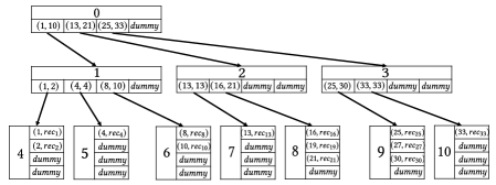
To delete a key-record pair in a B+ tree in , we do a classical search to find the leaf that contains and replace the key-record pair with a . Then, we check if its ancestors are still balanced. If an imbalanced ancestor is found, we first check if it can borrow a child from its sibling. Figure 2(a) shows an example in this case. Otherwise, we check if it can be directly merged with its sibling, which indicates that the node and its sibling have at most children. If not, we merge the node and its sibling by rebuilding the subtrees below them. Figure 2(b) shows an example in this case. Then, after rebalancing the B+ tree, we check if the root node still has at least two children. If not, we check if it can borrow a child from another B+ tree in . If not, then if there are at least two B+ trees in , we merge the root nodes of the two B+ trees. Otherwise, we remove the root node and downgrade the B+ tree from to .
The following lemma shows that the insertions and deletions in the quantum B+ tree is efficient.
Lemma 5.1.
The amortized cost of an insertion or a deletion in a dynamic quantum B+ tree is .
By Theorem 3.1 in (bentley1980decomposable), insertions totally cost time. Therefore, the amortized cost of one insertion is . For deletions, the first step costs time, since it consists of two point queries in B+ trees. By the analysis of partial rebuilding in (overmars1983design), the second step also costs time. Therefore, the amortized cost of a deletion is .
5.1.2. Query
To answer a query on our dynamic quantum B+ tree, we extend our idea of the GCLQ algorithm to perform both a global classical search and a local quantum search on the forests .
First, for global classical search, we follow the similar global search steps as introduced in Section 4.2 for each tree in the forests. Specifically, we first create an empty list for each forest (), and we add all the root nodes in into . Then, for each list , we perform a global classical search from each root in . A candidate set of at most two nodes are returned for each root, which are then added to the original list for easier processing.
Then, we perform the local quantum search for the candidate nodes in the lists . Consider the nodes in the lists, where is the total number of nodes in . We initialize the quantum bits to be where is the height of , and is the normalized amplitude of each such that each of the key-record pair below the nodes in the lists has the same amplitude in the result. Then, we do the same steps in Section 4.2.2 to obtain the leaves below the nodes. Finally, we do a post-selection search as discussed in Section 4.2.
The following theorem shows the time complexity for the dynamic quantum B+ tree to answer a quantum range query.
Theorem 5.2.
On average, the dynamic quantum B+ tree answers a range query in time.
The global classical search costs time, since we have forests and the global search for each forest needs time. For the local quantum search, the initialization and the steps to obtain the leaves cost . The average number of post-selection is , since there are at most nodes in the lists. Totally, the time complexity is .
5.2. Quantum Range Tree
In this section, we consider the multi-dimensional quantum range query. The range tree (bentley1978decomposable) is a common data structure for the classical multi-dimensional range query. It answers a -dimensional range query in time. For the multi-dimensional quantum range query, we extend our mechanism of the static quantum B+ tree to form the static quantum range tree. Similarly, our static quantum range tree improves the complexity to , which saves the part compared with the classical range tree.
We construct a quantum range tree by induction. To build a -dimensional quantum range tree, we first build a classical B+ tree indexing the -th dimension of the keys. Then, we build a -dimensional tree for each internal node in the B+ tree based on the key-record pairs below the internal node. Specially, a -dimensional quantum range tree is a static quantum B+ tree. Obviously, the space complexity and the time complexity of the construction are similar to the classical range tree.
Then, we discuss the -dimensional quantum range query. Starting from the -th dimension, we search the B+ tree and find the internal nodes in the search path which covers the -th dimension of the query range. Then, we turn to the quantum range trees on the internal nodes and do a -dimensional range search. Similar to the classical range tree, we then fetch the answers in -dimensional quantum range trees.
In the following theorem, we also show the time complexity of answering the -dimensional quantum range query with our proposed quantum range tree.
Theorem 5.3.
On average, the quantum range tree answers a -dimensional quantum range query in time.
The first step to obtain the 1D quantum range trees costs time. The second step to perform a global classical search on the quantum B+ tree costs time. The third step to perform a local quantum search starting from candidate nodes costs time. Overall, the average time complexity is .
6. Experiment
In this section, we show our experimental results to verify the superiority of our proposed quantum B+ tree on quantum range queries. The study of the real-world quantum supremacy (arute2019quantum; boixo2018characterizing; terhal2018quantum), which is to confirm that a quantum computer can do tasks faster than classical computers, is still a developing topic in the quantum area. Thus, in this paper, we would not verify the quantum supremacy, which we believe will be fully verified in a future quantum computer. To the best of our knowledge, there exists no information about the real implementation of the quantum memory (i.e., QRAM) that can suggest the execution time of algorithms on quantum computers. Therefore, we chose to evaluate the number of memory accesses to make the comparisons, which corresponds to IOs in traditional searches. In the quantum data structures, a QRAM read or write operation is counted as 1 IO (following the assumption of the load/store operation in QRAM (kerenidis2017quantum; saeedi2019quantum)). In the classical data structures, a page access is counted as 1 IO as well. Moreover, although there exist some quantum simulators such as Qiskit (wille2019ibm) and Cirq (cirq), they are not capable of simulating an efficient QRAM, and thus we chose to use C++ to perform the quantum simulations.
We used two real datasets from SNAP (leskovec2016snap), namely Brightkite and Gowalla. Each of the two datasets contains a set of check-in records, each of which consists of a timestamp (i.e., an integer) and a location (i.e., a 2-tuple of integers). The original sizes of the two datasets are 4M and 6M, respectively. For the 1-dimensional static and dynamic quantum range queries, we set the timestamp as the search key. For the multi-dimensional quantum range query, we set the location as the 2-dimensional search key.
For the 1-dimensional static and dynamic quantum range queries, we compare our GCLQ search algorithm on our proposed quantum B+ tree and its dynamic variant (which are simply denoted as quantum B+ tree) with the classical B+ tree search algorithm and its dynamic version (bentley1980decomposable) (which are denoted as classical B+ tree). For the multi-dimensional quantum range queries, we also compare our search algorithm on the proposed quantum range tree (which is denoted as quantum range tree) with the search on the classical range tree (chazelle1990lower1) (which is denoted as classical range tree). Note that the classical range tree is shown to be asymptotically optimal to solve the multi-dimensional range queries on classical computers.
The factors we studied are the dataset size , the branching factor and the selectivity (which is defined to be the proportion of items within the query range among the entire dataset). We varied from 4K to 2M (by randomly choosing a subset from each dataset with the target size). We varied from 4 to 64 for each data structure. We varied the selectivity from 1% to 10%. By default, 2M, 16 and the selectivity is 5%. For each type of range query, we randomly generate 10000 range queries and report the average measurement.
We present our experimental results as follows. For the sake of space, we mainly show the results of dataset Brightkite, while we observe similar results in the other dataset Gowalla in all our experiments. The complete results of dataset Gowalla can be found in our technical report (technical_report).

|

|

|

|

|
|---|---|---|---|---|
| (a) Brightkite | (b) Gowalla | (c) Brightkite | (d) Brightkite | (e) Brightkite |

|

|
| (a) Brightkite | (b) Brightkite |

|

|
| (c) Brightkite | (d) Brightkite |
Effect of . We first study the effect of the dataset , which verifies the scalability of our proposed data structures and algorithms. As shown in Figures 3(a) and (b), our proposed quantum B+ tree with our proposed GCLQ search algorithm scales well when grows from 4K to 2M on both datasets, which verifies the efficient cost of performing the GCLQ search on our quantum B+ tree. As increases, the number of items within the query range (i.e., ) for each query also tend to increase (approximately linearly with ). Thus, the number of memory access for the classical B+ tree demonstrates a linear growth with , which complies its complexity. In comparison, the performance of our quantum B+ tree does not depend on the number of range query results, and thus it is up to 1000x more efficient than the classical B+ tree for the (static) quantum range queries.
For multi-dimensional quantum range queries, our proposed quantum range tree obtains superior performance than the classical range tree similarly, as shown in Figure 3(c). For the dynamic quantum range queries, although our (dynamic) quantum B+ tree has larger number of memory accesses than the (dynamic) classical B+ tree for small (i.e., 100K), our quantum B+ tree shows much better scalability for larger , as illustrated in Figure 3(d). For the dynamic versions, we also tested the performance of insertions and deletions. Following (alsubaiee2014storage), we insert all the records in the datasets where for each insertion, there is 1% chance to delete an existing record instead of doing this insertion, and we measure the number of memory accesses for each insertion or deletion operation on average. Figure 3(e) shows that the dynamic quantum B+ tree needs 3x more memory accesses for insertion or deletion, because the quantum B+ tree has more complex structure than the classical B+ tree. However, the quantum B+ tree shows the growth, which is similar to the classical B+ tree, indicating that the insertion and deletions operations on our quantum B+ tree are still reasonably efficient.
Effect of Selectivity. Then, we study the effect of selectivity on the quantum range queries. When the selectivity (i.e., ) increases from 1% to 10% for both the static and the dynamic quantum range queries (as shown in Figures 4(a) and (c)), the number of memory accesses increases linearly for the classical B+ tree due to the query complexity. Our proposed quantum B+ tree with cost surprisingly shows better performance as the selectivity increases. This is because a larger shortened the process of the classical global search in our GCLQ search algorithm, such that the efficient local quantum search can be triggered earlier. Also, when increases, the post-selection will be accelerated since the cost of post-selection is linear to as we mentioned in Section 4.2.
In the multi-dimensional quantum range queries, as shown in Figure 5(a), although the number of memory accesses of our quantum range tree does not decrease as the selectivity increases (because a larger leads to more candidate nodes from global classical search in the multi-dimensional case), our quantum range tree is still efficient (since its performance does not depend on the selectivity) and is 10x–100x superior than the classical range tree.

|

|
|---|---|
| (a) Brightkite | (b) Brightkite |
Effect of . We also study the effect of the branching factor . As shown in Figures 4(b), 4(d) and 5(b), when increases, the number of memory accesses for the classical data structures decreases sharply, since the height of the tree is smaller for larger . Our quantum data structures needs slightly more memory accesses as increases, because the success rate of the post-selection could be affected as we mentioned in Section 4.2.2. However, it is well known that a larger branching factor leads to more memory consumption for a classical B+ tree (comer1979ubiquitous) (and thus a quantum B+ as well). Thus, we set to be 16 in other experiments for fair comparisons with a reasonable memory consumption. Overall, our proposed quantum data structures favor a smaller branching factor.
Summary. In summary, our quantum B+ tree with our proposed GCLQ search algorithm achieves up to 1000x performance improvement than the classical B+ tree. On the dataset Brightkite of size 2M, the average number of memory access is only around 40 for the quantum B+ tree for the quantum range query, while the classical B+ tree needs around 40K memory accesses. The similar superiority of our quantum B+ tree is observed on the dynamic and multi-dimensional quantum range queries compared with the classical data structures. We also show that our quantum B+ tree scales well with the dataset size, the selectivity of the query ranges and the branching factor.
7. Related Work
The classical range query problem has been studied for decades with various data structures proposed to solve this problem. There is little room for further significant improvement. For the static range query and the dynamic range query, the B-tree (bayer2002organization) and the B+ tree (comer1979ubiquitous) are widely-used. The B+ tree is a tree data structure which can find a key in time, where is the number of key-record pairs and is the branching factor. Then, time is needed to load the key-record pairs in the query range, so the range query on a B+ tree costs time, which is shown to be asymptotically optimal in classical computers (yao1981should).
For the high-dimensional static range query, Bentley (bentley1978decomposable) proposed the range tree to answer it in time, where is the dimension of the keys. In addition, the range tree needs storage space. Chazelle later (chazelle1990lower1; chazelle1990lower2) proposed the lower bounds for the -dimensional cases: time complexity with storage space and time complexity with units storage space where the lower bound of query I/O cost is provably tight for .
However, all the above classical data structures have the same problem that the execution time grows linearly with , which makes them useless for quantum algorithms.
The quantum database searching problem is also very popular in the quantum algorithm field. Grover’s algorithm is described as a database search algorithm in (grover1996fast). It solves the problem of searching a marked record in an unstructured list, which means that all the records are arranged in random order. On average, the classical algorithm needs to perform queries to a function which tells us if the record is marked. More formally, for each index , means the -th record is marked and means the -th record is unmarked. Note that only one record is marked in the database. Taking the advantage of quantum parallelism, Grover’s algorithm can find the index of the marked record with queries to the oracle. The main idea is to first “flip” the amplitude of the answer state and then reduce the amplitudes of the other states. One such iteration will enlarge the amplitude of the answer state and iterations should be performed until the probability that the qubits are measured to be the answer comes close to 1. Then, an improved Grover’s algorithm was proposed in (boyer1998tight). We are also given the function to mark the record, but records are marked at this time. The improved Grover’s algorithm can find one of the marked records in time. If we make the function to mark the records with keys within a query range, then this algorithm returns one of the key-record pairs in time, and it needs time to answer a range query. Since the query time grows linearly with the square root of , this algorithm is much less efficient when is very large, even compared to using the classical data structure with time complexity. The reason is that this algorithm only handle the unstructured dataset and does not leverage the power of data structures that could be pre-built as a database index.
In the database area, there are also plenty of studies discussing how to use quantum computers to further improve traditional database queries. For example, (uotila2022synergy; schonberger2022applicability; fankhauser2021multiple; trummer2015multiple) discussed quantum query optimization, which is to use quantum algorithms like quantum annealing (finnila1994quantum) to optimize a traditional database query. However, compared with the quantum range query discussed in this paper, the existing studies are in a different direction. The existing studies are discussing how to use a quantum algorithm to optimize range queries in a classical computer, where the query returns a list of records. In this paper, we discuss how to use a classical algorithm to optimize range queries in a quantum computer, where the query returns quantum bits in a superposition of records. We focus on a quantum data structure stored in a quantum computer, where the classical algorithm is only to assist the query. To our best knowledge, in the database area, we are the first to discuss quantum algorithms in this direction.
In conclusion, the existing classical data structures and the existing quantum database searching algorithms cannot solve the range query problem in quantum computers perfectly.
8. Conclusion
In this paper, we study the quantum range query problem. We propose the quantum B+ tree, the first tree-like quantum data structure, and the efficient global-classical local-quantum search algorithm based on the quantum B+ tree. Our proposed data structure and algorithm can answer a quantum range query in time, which is asymptotically optimal in quantum computers and is exponentially faster than classical B+ trees. Furthermore, we extend it to a dynamic quantum B+ tree. The dynamic quantum B+ tree can support insertions and deletions in time and answer a dynamic quantum range query in time. We also extend the quantum B+ tree to the quantum range tree to solve the -dimensional quantum range query in time. In the experiments, we did simulations to verify the superiority of our proposed quantum data structures compared with the classical data structures. We expect that the quantum data structures will show significant advantages in the real world.
The future work includes exploring even more efficient quantum algorithms for the dynamic and multi-dimensional range queries and studying more advanced database queries such as the top- queries.
References
- (1)
- Abohashima et al. (2020) Zainab Abohashima, Mohamed Elhosen, Essam H Houssein, and Waleed M Mohamed. 2020. Classification with Quantum Machine Learning: A Survey. arXiv e-prints (2020), arXiv–2006.
- Adhikary et al. (2020) Soumik Adhikary, Siddharth Dangwal, and Debanjan Bhowmik. 2020. Supervised learning with a quantum classifier using multi-level systems. Quantum Information Processing 19, 3 (2020), 1–12.
- Alsubaiee et al. (2014) Sattam Alsubaiee, Alexander Behm, Vinayak Borkar, Zachary Heilbron, Young-Seok Kim, Michael J Carey, Markus Dreseler, and Chen Li. 2014. Storage management in AsterixDB. Proceedings of the VLDB Endowment 7, 10 (2014), 841–852.
- Ambainis (1999) Andris Ambainis. 1999. A better lower bound for quantum algorithms searching an ordered list. In 40th Annual Symposium on Foundations of Computer Science (Cat. No. 99CB37039). IEEE, 352–357.
- Arge and Vitter (1996) Lars Arge and Jeffrey Scott Vitter. 1996. Optimal dynamic interval management in external memory. In Proceedings of 37th Conference on Foundations of Computer Science. IEEE, 560–569.
- Arute et al. (2019) Frank Arute, Kunal Arya, Ryan Babbush, Dave Bacon, Joseph C Bardin, Rami Barends, Rupak Biswas, Sergio Boixo, Fernando GSL Brandao, David A Buell, et al. 2019. Quantum supremacy using a programmable superconducting processor. Nature 574, 7779 (2019), 505–510.
- Author(s) (2023) Anonymous Author(s). 2023. First Tree-like Quantum Data Structure: Quantum B+ Tree. Technical Report. https://github.com/anonym45263/EBDE402C7C7404A8
- Bayer and McCreight (2002) Rudolf Bayer and Edward McCreight. 2002. Organization and maintenance of large ordered indexes. In Software pioneers. Springer, 245–262.
- Benedetti et al. (2019) Marcello Benedetti, Delfina Garcia-Pintos, Oscar Perdomo, Vicente Leyton-Ortega, Yunseong Nam, and Alejandro Perdomo-Ortiz. 2019. A generative modeling approach for benchmarking and training shallow quantum circuits. npj Quantum Information 5, 1 (2019), 1–9.
- Bentley (1978) Jon Louis Bentley. 1978. Decomposable searching problems. Technical Report. CARNEGIE-MELLON UNIV PITTSBURGH PA DEPT OF COMPUTER SCIENCE.
- Bentley and Saxe (1980) Jon Louis Bentley and James B Saxe. 1980. Decomposable searching problems I. Static-to-dynamic transformation. Journal of Algorithms 1, 4 (1980), 301–358.
- Berg et al. (2021) Axel Berg, Magnus Oskarsson, and Mark O’Connor. 2021. Deep ordinal regression with label diversity. In 2020 25th International Conference on Pattern Recognition (ICPR). IEEE, 2740–2747.
- Boixo et al. (2018) Sergio Boixo, Sergei V Isakov, Vadim N Smelyanskiy, Ryan Babbush, Nan Ding, Zhang Jiang, Michael J Bremner, John M Martinis, and Hartmut Neven. 2018. Characterizing quantum supremacy in near-term devices. Nature Physics 14, 6 (2018), 595–600.
- Boyer et al. (1998) Michel Boyer, Gilles Brassard, Peter Høyer, and Alain Tapp. 1998. Tight bounds on quantum searching. Fortschritte der Physik: Progress of Physics 46, 4-5 (1998), 493–505.
- Brassard et al. (1998) Gilles Brassard, Peter Høyer, and Alain Tapp. 1998. Quantum counting. In International Colloquium on Automata, Languages, and Programming. Springer, 820–831.
- Campos et al. (2010) Pedro G Campos, Alejandro Bellogín, Fernando Díez, and J Enrique Chavarriaga. 2010. Simple time-biased KNN-based recommendations. In Proceedings of the Workshop on Context-Aware Movie Recommendation. 20–23.
- Chakraborty et al. (2020) Sanjay Chakraborty, Soharab Hossain Shaikh, Amlan Chakrabarti, and Ranjan Ghosh. 2020. A hybrid quantum feature selection algorithm using a quantum inspired graph theoretic approach. Applied Intelligence 50, 6 (2020), 1775–1793.
- Chazelle (1990a) Bernard Chazelle. 1990a. Lower bounds for orthogonal range searching: I. the reporting case. Journal of the ACM (JACM) 37, 2 (1990), 200–212.
- Chazelle (1990b) Bernard Chazelle. 1990b. Lower bounds for orthogonal range searching: II. The arithmetic model. Journal of the ACM (JACM) 37, 3 (1990), 439–463.
- Comer (1979) Douglas Comer. 1979. Ubiquitous B-tree. ACM Computing Surveys (CSUR) 11, 2 (1979), 121–137.
- Covington et al. (2016) Paul Covington, Jay Adams, and Emre Sargin. 2016. Deep neural networks for youtube recommendations. In Proceedings of the 10th ACM conference on recommender systems. 191–198.
- Dirac (1939) Paul Adrien Maurice Dirac. 1939. A new notation for quantum mechanics. In Mathematical Proceedings of the Cambridge Philosophical Society, Vol. 35. Cambridge University Press, 416–418.
- Dougherty et al. (1995) James Dougherty, Ron Kohavi, and Mehran Sahami. 1995. Supervised and unsupervised discretization of continuous features. In Machine learning proceedings 1995. Elsevier, 194–202.
- Durr and Hoyer (1996) Christoph Durr and Peter Hoyer. 1996. A quantum algorithm for finding the minimum. arXiv preprint quant-ph/9607014 (1996).
- Fankhauser et al. (2021) Tobias Fankhauser, Marc E Solèr, Rudolf M Füchslin, and Kurt Stockinger. 2021. Multiple query optimization using a hybrid approach of classical and quantum computing. arXiv preprint arXiv:2107.10508 (2021).
- Finnila et al. (1994) Aleta Berk Finnila, MA Gomez, C Sebenik, Catherine Stenson, and Jimmie D Doll. 1994. Quantum annealing: A new method for minimizing multidimensional functions. Chemical physics letters 219, 5-6 (1994), 343–348.
- Gidney C and contributors (2018) Bacon D Gidney C and contributors. 2018. Cirq: A python framework for creating, editing, and invoking noisy intermediate scale quantum (NISQ) circuits. https://github.com/quantumlib/Cirq.
- Grover (1996) Lov K Grover. 1996. A fast quantum mechanical algorithm for database search. In Proceedings of the twenty-eighth annual ACM symposium on Theory of computing. 212–219.
- Grover and Radhakrishnan (2005) Lov K Grover and Jaikumar Radhakrishnan. 2005. Is partial quantum search of a database any easier?. In Proceedings of the seventeenth annual ACM symposium on Parallelism in algorithms and architectures. 186–194.
- Gupta and Singh (2013) Anant Gupta and Kuldeep Singh. 2013. Location based personalized restaurant recommendation system for mobile environments. In 2013 International Conference on Advances in Computing, Communications and Informatics (ICACCI). IEEE, 507–511.
- Hadamard (1893) Jacques Hadamard. 1893. Resolution d’une question relative aux determinants. Bull. des sciences math. 2 (1893), 240–246.
- Harrow et al. (2009) Aram W Harrow, Avinatan Hassidim, and Seth Lloyd. 2009. Quantum algorithm for linear systems of equations. Physical review letters 103, 15 (2009), 150502.
- Hosoyamada and Sasaki (2018) Akinori Hosoyamada and Yu Sasaki. 2018. Quantum Demiric-Selçuk meet-in-the-middle attacks: applications to 6-round generic Feistel constructions. In International Conference on Security and Cryptography for Networks. Springer, 386–403.
- Ibtehaz et al. (2021) Nabil Ibtehaz, M Kaykobad, and M Sohel Rahman. 2021. Multidimensional segment trees can do range updates in poly-logarithmic time. Theoretical Computer Science 854 (2021), 30–43.
- Kapralov et al. (2020) Ruslan Kapralov, Kamil Khadiev, Joshua Mokut, Yixin Shen, and Maxim Yagafarov. 2020. Fast Classical and Quantum Algorithms for Online -server Problem on Trees. arXiv preprint arXiv:2008.00270 (2020).
- Kerenidis and Prakash (2017) Iordanis Kerenidis and Anupam Prakash. 2017. Quantum Recommendation Systems. In 8th Innovations in Theoretical Computer Science Conference (ITCS 2017). Schloss Dagstuhl-Leibniz-Zentrum fuer Informatik.
- Kieferova et al. (2021) Maria Kieferova, Ortiz Marrero Carlos, and Nathan Wiebe. 2021. Quantum Generative Training Using R’enyi Divergences. arXiv preprint arXiv:2106.09567 (2021).
- Kim and Won (2001) Sang-Wook Kim and Hee-Sun Won. 2001. Batch-construction of B+-trees. In Proceedings of the 2001 ACM symposium on Applied Computing. 231–235.
- Leskovec and Sosič (2016) Jure Leskovec and Rok Sosič. 2016. Snap: A general-purpose network analysis and graph-mining library. ACM Transactions on Intelligent Systems and Technology (TIST) 8, 1 (2016), 1–20.
- Li et al. (2021a) Guangxi Li, Zhixin Song, and Xin Wang. 2021a. VSQL: variational shadow quantum learning for classification. In Proceedings of the AAAI Conference on Artificial Intelligence, Vol. 35. 8357–8365.
- Li et al. (2019) Tongyang Li, Shouvanik Chakrabarti, and Xiaodi Wu. 2019. Sublinear quantum algorithms for training linear and kernel-based classifiers. In International Conference on Machine Learning. PMLR, 3815–3824.
- Li et al. (2021b) Tongyang Li, Chunhao Wang, Shouvanik Chakrabarti, and Xiaodi Wu. 2021b. Sublinear Classical and Quantum Algorithms for General Matrix Games. In Proceedings of the AAAI Conference on Artificial Intelligence, Vol. 35. 8465–8473.
- Mitarai et al. (2018) Kosuke Mitarai, Makoto Negoro, Masahiro Kitagawa, and Keisuke Fujii. 2018. Quantum circuit learning. Physical Review A 98, 3 (2018), 032309.
- Montanaro (2017) Ashley Montanaro. 2017. Quantum pattern matching fast on average. Algorithmica 77, 1 (2017), 16–39.
- Naya-Plasencia and Schrottenloher (2020) María Naya-Plasencia and André Schrottenloher. 2020. Optimal Merging in Quantum -xor and -sum Algorithms. In Annual International Conference on the Theory and Applications of Cryptographic Techniques. Springer, 311–340.
- Nielsen and Chuang (2001) Michael A Nielsen and Isaac L Chuang. 2001. Quantum computation and quantum information. Phys. Today 54, 2 (2001), 60.
- Overmars (1983) Mark H Overmars. 1983. The design of dynamic data structures. Vol. 156. Springer Science & Business Media.
- O’Neil et al. (1996) Patrick O’Neil, Edward Cheng, Dieter Gawlick, and Elizabeth O’Neil. 1996. The log-structured merge-tree (LSM-tree). Acta Informatica 33, 4 (1996), 351–385.
- Rebentrost et al. (2014) Patrick Rebentrost, Masoud Mohseni, and Seth Lloyd. 2014. Quantum support vector machine for big data classification. Physical review letters 113, 13 (2014), 130503.
- Ruan et al. (2017) Yue Ruan, Xiling Xue, Heng Liu, Jianing Tan, and Xi Li. 2017. Quantum algorithm for k-nearest neighbors classification based on the metric of hamming distance. International Journal of Theoretical Physics 56, 11 (2017), 3496–3507.
- Saeedi and Arodz (2019) Seyran Saeedi and Tom Arodz. 2019. Quantum sparse support vector machines. arXiv preprint arXiv:1902.01879 (2019).
- Schönberger (2022) Manuel Schönberger. 2022. Applicability of quantum computing on database query optimization. In Proceedings of the 2022 International Conference on Management of Data. 2512–2514.
- Schrödinger (1935) Erwin Schrödinger. 1935. Discussion of probability relations between separated systems. In Mathematical Proceedings of the Cambridge Philosophical Society, Vol. 31. Cambridge University Press, 555–563.
- Schuld et al. (2020) Maria Schuld, Alex Bocharov, Krysta M Svore, and Nathan Wiebe. 2020. Circuit-centric quantum classifiers. Physical Review A 101, 3 (2020), 032308.
- Schuld and Killoran (2019) Maria Schuld and Nathan Killoran. 2019. Quantum machine learning in feature Hilbert spaces. Physical review letters 122, 4 (2019), 040504.
- Sen and Venkatesh (2001) Pranab Sen and Srinivasan Venkatesh. 2001. Lower bounds in the quantum cell probe model. In International Colloquium on Automata, Languages, and Programming. Springer, 358–369.
- Shor (1994) Peter W Shor. 1994. Algorithms for quantum computation: discrete logarithms and factoring. In Proceedings 35th annual symposium on foundations of computer science. Ieee, 124–134.
- Terhal (2018) Barbara M Terhal. 2018. Quantum supremacy, here we come. Nature Physics 14, 6 (2018), 530–531.
- Trummer and Koch (2015) Immanuel Trummer and Christoph Koch. 2015. Multiple query optimization on the D-Wave 2X adiabatic quantum computer. arXiv preprint arXiv:1510.06437 (2015).
- Uotila (2022) Valter Uotila. 2022. Synergy between Quantum Computers and Databases. (2022).
- Wiebe et al. (2015) Nathan Wiebe, Ashish Kapoor, and Krysta M Svore. 2015. Quantum algorithms for nearest-neighbor methods for supervised and unsupervised learning. Quantum Information & Computation 15, 3-4 (2015), 316–356.
- Wille et al. (2019) Robert Wille, Rod Van Meter, and Yehuda Naveh. 2019. IBM’s Qiskit tool chain: Working with and developing for real quantum computers. In 2019 Design, Automation & Test in Europe Conference & Exhibition (DATE). IEEE, 1234–1240.
- Xue and Hauskrecht (2017) Yanbing Xue and Milos Hauskrecht. 2017. Efficient learning of classification models from soft-label information by binning and ranking. In The Thirtieth International Flairs Conference.
- Yao (1981) Andrew Chi-Chih Yao. 1981. Should tables be sorted? Journal of the ACM (JACM) 28, 3 (1981), 615–628.
- Zhang and Korepin (2018) Kun Zhang and Vladimir Korepin. 2018. Quantum partial search for uneven distribution of multiple target items. Quantum Information Processing 17, 6 (2018), 1–20.

|

|

|

|
|---|---|---|---|
| (a) Gowalla | (b) Gowalla | (c) Gowalla | (d) Gowalla |

|

|
| (a) Gowalla | (b) Gowalla |

|

|
| (c) Gowalla | (d) Gowalla |

|

|
|---|---|
| (a) Gowalla | (b) Gowalla |
Appendix A Remaining Experimental Results
In this section, we show the complete experimental results of dataset Gowalla, which are not presented in Section 6 due to the space limit.
Appendix B Complete Proofs
In this section, we show the complete proofs of all the lemmas and theorems in this paper.
Proof of Lemma 4.2.
Consider a static quantum range query . It answers whether the key exists in the dataset, which is a static membership problem. By (sen2001lower), the time complexity of answering a static membership problem in quantum computers is . Therefore, the time complexity of answering a static quantum range query is also . ∎
Proof of Lemma 4.3.
Since the routing keys of all nodes in the same level are disjoint, we cannot have more than two partial nodes in the same level. It is also easy to verify that the returned nodes are from the same level, Thus, the candidate set contains at most two nodes. Since we only filter out the outside node in this algorithm, we have . Finally, since the precise partial node either is a leaf (which contains at least items in the query range), or contains an inside child (which contains at least items in the query range due to the balanced nodes of the B+ tree), and it can be verify that at least one returned node is precise, we have . ∎
Proof of Lemma 4.4.
The global classical search costs time because we return at most two candidates and the height of the tree is . For the local quantum search, we repeat all the steps for times on average. By the condition to trigger a local quantum search, all the non-dummy key-record pairs below one of the children of and are all in the answer, therefore by the definition of our quantum B+ tree. So, we need to repeat all the steps for at most times, which is a constant time. In each iteration, we do Step 2 and Step 3 for at most times, so the local quantum search needs time. Therefore, the quantum range query algorithm needs time. ∎
Proof of Theorem 5.1.
By Theorem LABEL:theo1 in this paper and Theorem 3.1 in (bentley1980decomposable), insertions totally cost time. Therefore, the amortized cost of one insertion is .
To analyze the update cost in a merge, we have that when merging , the time complexity to update is . The reason is as follows.
Let denote the least ID in . For each and each key-record pair in , the ID of the key-record pair is smaller than . Let denote the greatest ID in . Then, for each and each key-record pair in , the ID of the key-record pair is greater than . Therefore, the update operations for the key-record pairs in can be merged into a range update. Then, we can use lazy propagation (ibtehaz2021multidimensional) to do the range update in time.
Thus, the extra cost to maintain and has no impact, which means the amortized cost of insertion is still .
For deletions, the first step costs time, since it consists of two point queries in B+ trees.
Then consider the second step. Motivated by the analysis of partial rebuilding in (overmars1983design), we consider a node of height just after a rebuild. The node is perfectly balanced such that its weight . Since it will become imbalanced if and only if , there must be deletions below the node or its siblings before that. So, it is charged time for each deletion below it and its siblings. Then, for a deletion in a leaf node, each ancestor and its siblings are charged time, so they are totally charged time.
Therefore, the amortized cost of a deletion is .
∎
Proof of Theorem 5.2.
As above mentioned, the global classical search costs time. Consider the cost of the local quantum search. The initialization and the steps to obtain the leaves cost . Then, we multiply it by the average post-selection times. Let denote the total number of key-record pairs below the nodes in . Then, the post-selection needs to be iterated times on average. Since there are at most nodes in the lists and each node has a weight at most , we have . Before we turn to the local quantum search, we have found a child of a node in such that all the key-record pairs below the child are in the answer, such that . Therefore, . Hence, the local quantum search costs time on average.
Since both the global classical search and the local quantum search cost time, the dynamic quantum B+ tree answers a range query in time on average. ∎
Proof of Theorem 5.3.
The first step is to recursively search the quantum range trees to obtain the -dimensional quantum range trees which contain answers. It costs time. The second step is to perform a global classical search on the quantum B+ tree. It costs time. The third step is to perform a local quantum search starting from candidate nodes returned in the second step. We first initialize the quantum bits in time. Then, we do the same Step 2 and Step 3 in Section LABEL:local to obtain the leaves below the candidate nodes in time. Thus, we need to do a constant number of post-selections. Therefore, this step costs time.
Therefore, the quantum range tree answers a range query in time on average. ∎