Differentially Private Boxplots
Abstract
Despite the potential of differentially private data visualization to harmonize data analysis and privacy, research in this area remains relatively underdeveloped. Boxplots are a widely popular visualization used for summarizing a dataset and for comparison of multiple datasets. Consequentially, we introduce a differentially private boxplot. We evaluate its effectiveness for displaying location, scale, skewness and tails of a given empirical distribution. In our theoretical exposition, we show that the location and scale of the boxplot are estimated with optimal sample complexity, and the skewness and tails are estimated consistently. In simulations, we show that this boxplot performs similarly to a non-private boxplot, and it outperforms a boxplot naively constructed from existing differentially private quantile algorithms. Additionally, we conduct a real data analysis of Airbnb listings, which shows that comparable analysis can be achieved through differentially private boxplot visualization.
1 Introduction
It is now well established that differential privacy (Dwork et al.,, 2006) is a powerful framework for protecting the privacy of individuals’ data. As a result, a plethora of differentially private data analysis tools have been developed over the last several decades (Dwork,, 2008; Ji et al.,, 2014; Liu et al.,, 2023). However, one area that has been considerably underdeveloped is that of differentially private visualization. This is despite the fact that data visualization is a key tool in exploratory analysis, which is an essential component of data analysis. In fact, in a recent study of data analysts and practitioners, Garrido et al., (2023) found that “most analysts employed aggregations and visualizations to fulfill their use case,” rather than machine learning models.
Differentially private versions of several popular visualizations have been considered in the literature. There has been substantial study of the differentially private histogram (Hay et al.,, 2010; Li et al.,, 2010; Acs et al.,, 2012; Kellaris and Papadopoulos,, 2013; Xu et al.,, 2013; Zhang et al.,, 2014; Budiu et al.,, 2022). Visualizations based on clustering (Hongde et al.,, 2014), for mobility data (He et al.,, 2016), heatmaps (Zhang et al.,, 2016) and scatterplots (Panavas et al.,, 2024) have also been considered.
Surprisingly, despite its widespread use, a differentially private boxplot has not been directly studied. Boxplots, invented by Tukey et al., (1977), are used for visualizing the characteristics of a univariate sample, as well as for visualizing the relationship between a continuous variable and a categorical variable. Despite its simplicity, many key distributional characteristics can be evaluated from the boxplot: namely, location, scale, skewness, and tails. This has made it popular among practitioners.
In addition, its simplicity is beneficial from a privacy standpoint. The boxplot only requires estimating a few summary statistics in order to convey the distributional characteristics of a univariate sample, making the boxplot efficient in its use of privacy budget. For instance, by contrast, a histogram can also be used to convey the same information. However, a histogram is generally a consistent estimate of the population density, which intuitively, should then require more noise to ensure privacy.
Motivated by these observations, we develop and study a differentially private boxplot. Our contributions are as follows: We introduce a differentially private boxplot and evaluate its ability to convey location, scale, skewness and tails both theoretically and empirically. We show that the inner quantiles used for the location and scale of the boxplot are estimated optimally (Theorem 2). We then show that tails and skewness are estimated consistently (Theorem 5). Through extensive simulations, we show that the proposed boxplot is often more accurate than one naively constructed via popular, existing differentially private quantile methods (see Section 5). We also conduct a differentially private exploratory data analysis, demonstrating the utility of the proposed boxplots, as well as their limitations (see Section 6). As a by-product of our work, we develop some new results concerning private quantiles. We introduce a minimax lower bound on private quantile estimation, and show that when the number of quantiles is small, the quantile algorithms JointExp (Gillenwater et al.,, 2021) and PrivateQuantile (Smith,, 2011) attain this lower bound, up to logarithmic factors. We also theoretically confirm the empirical observation of Durfee, (2023), which says that the unbounded quantile algorithm performs better than existing algorithms for estimating extreme quantiles. We show that JointExp is inconsistent for extreme quantiles (Lemma 9), where the unbounded algorithm of Durfee, (2023) is consistent (Lemma 8). We also present simulations comparing four differentially private quantile algorithms, those of Smith, (2011); Gillenwater et al., (2021); Kaplan et al., (2022) and Durfee, (2023).
Before turning to our main results, we mention some other related works. Nanayakkara et al., (2022) developed a plot to visualize privacy utility trade-offs. Zhou et al., (2022) developed DPVisCreator, a visualization system, which relies on publishing a synthetic dataset. Visualizations in other privacy models were considered by Dasgupta and Kosara, (2011); Dasgupta et al., (2013, 2019), and recently reviewed by Bhattacharjee et al., (2020). In addition, a related area is that of differentially private quantile estimation (Smith,, 2011; Gillenwater et al.,, 2021; Kaplan et al.,, 2022; Alabi et al.,, 2022; Durfee,, 2023; Lalanne et al., 2023a, ; Lalanne et al., 2023b, ). One could apply any one of these algorithms to create a differentially private boxplot. We show in Section 5 that this approach is often less accurate than the proposed methodology.
2 Preliminaries
First, we briefly review the boxplot. We define a dataset of size to be a set of real numbers of size . Let be the set of datasets of size and let be a dataset size . The boxplot consists of a box with a line drawn through it, with two whiskers emanating from the lower and upper bounds of the box. Specific points are sometimes indicated above or below the whiskers. The central line inside the box marks the median of the dataset. The box itself is constructed from the quartiles, detailing the middle 50% of . The lower (upper) whisker is constructed from the larger (smaller) of the minimum (maximum) of and the lower (upper) quartile of minus (plus) 1.5 times the interquartile range of . Lastly, any points in falling outside of the whiskers are added to the plot. See Figure 2 for an example. The boxplot describes various characteristics of . The median line approximates the location of . The box itself approximates the spread or scale of . The skewness of can be approximated as follows: A median line placed in the center of the box, along with whiskers that are similar in magnitude, suggests a symmetric distribution. A median line placed away from the center of the box or asymmetric whiskers indicates skewness. Additionally, the tails can be assessed by the number of points beyond the whiskers. Many such points signify outliers or heavy tails, highlighting data points that deviate significantly from the rest.
Next, we introduce differential privacy. First, we say that , is adjacent to if and differ in exactly one point. Let be the set of pairs of adjacent datasets of size . Next, denote by a probability measure which depends on . For a space , let denote the Borel sets of and let be the set of Borel probability measures over . Formally, is a map from to , for some . We can now define differential privacy.
Definition 1.
The quantity is -differentially private if
| (1) |
Here, is a -dimensional differentially private quantity and is the privacy budget, where values of which are closer to zero enforce stricter privacy constraints.
The proposed differentially private boxplot makes use of existing differentially private algorithms. Specifically, the Laplace mechanism, and algorithms for computing differentially private quantiles. The Laplace mechanism (Dwork et al.,, 2006) is a fundamental mechanism for constructing differentially private statistics. Let be a standard Laplace random variable. Specifically, for a statistic , define its global sensitivity to be . If has global sensitivity bounded by 1, then is a differentially private quantity. This is known as the Laplace mechanism.
Of course, a private boxplot relies on differentially private quantiles. The proposed private boxplot relies on the unbounded algorithm of Durfee, (2023) and the JointExp algorithm of Gillenwater et al., (2021). These algorithms are the main focus of our theoretical exposition. We do, however, consider the performance of the naive boxplot constructed via the algorithms of Smith, (2011), Kaplan et al., (2022) and Durfee, (2023) in our simulation study, see Section 5. We also discuss the extent to which our theoretical results extend to these other algorithms, see Remark 4.
We now give a brief overview of JointExp and unbounded. JointExp works as follows: Suppose we wish to estimate quantiles of levels . For an integer , let denote the set . Define the th quantile generated by JointExp for a given to be , and let . For a given , let be the cumulative distribution function of and, if it exists, let be its probability density function. Now, define the following utility function: where , and . Then has law , where It was shown by Gillenwater et al., (2021) that is -differentially private. Furthermore, Lalanne et al., 2023b showed that this algorithm is consistent for continuous distributions. If one suspects that the population distribution contains atoms, then we recommend that one uses the jittering modification proposed by Lalanne et al., 2023b . We show in Section 4 that this algorithm has optimal sample complexity for estimating a single quantile, and therefore, for the scale and location of the boxplot. (Here we are only interested in estimating three quantiles, and so, how sample complexity scales in in not of particular concern.)
The unbounded algorithm produces a private quantile given a lower bound on the data. We present a slightly modified version, which performs better for extreme quantiles. For a given quantile and , let be independent, standard exponential random variables and let . Define . The quantile estimate generated by the unbounded algorithm is given by: . If , then, we apply the above procedure to the dataset , with input parameters and . It follows from (Durfee,, 2023) that this algorithm is -differentially private. In the proposed differentially private boxplot algorithm, we use unbounded to estimate the minimum and maximum of the dataset. For a measure , let be the associated th quantile, and . We show that if is an independent sample from , then when as , is weakly consistent for , and when as , is weakly consistent for , see Lemma 8. By contrast, we show that JointExp is inconsistent for , see Lemma 9. Instead of exponential noise, one could also use Laplace or Gumbel noise (Durfee,, 2023). We found this to make little difference in simulation, and so we only present the version which incorporates exponential noise.
3 A differentially private boxplot
We can now introduce the differentially private boxplot. Let and . Given lower and upper bounds on the data and 111If one does not wish to supply input bounds for the data, one can use the “fully unbounded” version of unbounded (Durfee,, 2023). However, in simulation, (see Section 5), we have observed that the procedure is still accurate, even when the input bounds are very loose., we first generate the minimum and maximum estimates using the unbounded algorithm, denoted by and . Next, we run JointExp with input bounds to generate . The box bounds and center line are then constructed from . Letting , and be a sequence decreasing to 0, the lower and upper whisker are defined as
respectively. To elaborate, the role of the minimum and the maximum of the dataset in a traditional boxplot is played by the estimated extreme quantiles and . Given that estimated extreme quantiles are more variable than the estimated inner quantiles, we set a given whisker equal to its associated extreme quantile only when that quantile is at least 100% shorter than the quantity based on the noisy interquartile range. We take and c=. Several others were tested in simulation, see Appendix B.2. Note that we use the unbounded algorithm because JointExp (and, by consequence, PrivateQuantile and ApproxQuantile) are inconsistent for estimating quantiles that satisfy , see Lemma 9.
A traditional boxplot also plots the observations which lie above and below the upper and lower whiskers, respectively. We cannot release such data points under the constraints of differential privacy. Instead, we plot a noisy version of the number of points above , denoted and below , denoted . These are generated via the Laplace mechanism, where it is easy to see that the count of observations above or below a threshold has global sensitivity 1. Lastly, we attribute less privacy budget for computing the outliers, as we deem these values to be of less interest than the box itself. We assign each noisy outlyingness number a privacy budget of . Together, these seven values make up the differentially private boxplot. See Figure 3 for an example of the proposed private boxplot. The algorithm, which we call DPBoxplot is summarized in Algorithm 1.
Remark 1 (On the tuning parameters).
Our algorithm contains several tuning parameters, which were chosen via simulation. That is, we chose a quantile, rather than a quantile, the constant and , which showed the best performance in our simulation study. See Appendix B.2 for simulation results concerning the tuning parameters.
4 Theoretical results
In this section, we derive several results concerning the different elements of the private boxplot. We now assume that the dataset consists of independent, identically distributed random variables drawn from a population measure . We first prove an upper bound on the sample complexity of the inner quantiles generated from JointExp. We then prove a minimax lower bound for privately estimating a quantile from a population measure lying in a general set, which matches the upper bound. We then prove that the whiskers and outlyingness numbers and are weakly consistent for their population counterparts.
We now define a boxplot rigorously, as a function of a measure on the set of real numbers, which is convenient mathematically. The non-private boxplot constructed from the data is taken to be the boxplot computed on the empirical measure of the dataset , denoted by . For a measure , let be the associated th quantile, , and . For a measure , let . For , we let () be the minimum (maximum) of and . Now, letting and , the whiskers are defined as and Lastly, we can define , . The ‘population’ boxplot is the following seven number summary . Similarly, we can define the differentially private boxplot .
For and , let be the set of absolutely continuous measures such that . Our first result gives an upper bound on the sample complexity of the private quantiles generated via JointExp. For and , let and define .
Theorem 2.
For and so that , if is such that and , then there exists a universal constant such that for all and , it holds that with probability , provided that
The proof of Theorem 2 relies on a general bound for the exponential mechanism detailed by Ramsay et al., (2024), and so we defer it to Appendix A. Note that the upper bound given in Theorem 2 has suboptimal scaling in , the ApproxQuantile algorithm of Kaplan et al., (2022) obtains logarithmic scaling in . However, in this context, , and we are not so concerned about this fact.
Next, we present a minimax lower bound for estimating a single quantile subject to differential privacy, which in turn implies a lower bound for estimating quantiles. Again, since our main interest is in boxplot estimation, we are not concerned about optimal scaling in . Next, for a set , let be the set of maps from to which satisfy (1). Note is just a formal way of writing the set of all differentially private estimators which lie in . Let , and denote the minimax risk for differentially private quantile estimation by .
Theorem 3.
For all , , such that , it holds that
| (2) |
samples are required for to hold.
Note that Theorem 3 implies a lower bound on the sample complexity for estimating quantiles. That is, for all , , with , it holds that (2) samples are also required for . Applying this lower bound in conjunction with Theorem 2 yields that the scale and location of the proposed private boxplot are estimated optimally, up to logarithmic factors. Note that Tzamos and Vlatakis-Gkaragkounis, (2020) give a minimax lower bound on differentially private median estimation. Their result is similar, though the proof does not directly extend to estimating an arbitrary quantile, since it relies on a set of uniform distributions who have that the property that the median coincides with the mean. The proof of Theorem 3 is an elementary application of the differentially private version of Fano’s inequality (Acharya et al.,, 2021), it is deferred to Appendix A.
Remark 4.
Our theoretical exposition is based on JointExp, but any algorithm whose quantiles satisfy the same sample complexity bound given by Theorem 2 would result in optimal estimates of location and scale of the boxplot. For instance, PrivateQuantile of Smith, (2011) is a special case of JointExp, when only one quantile is being estimated, and therefore, the same results apply to PrivateQuantile. In addition, Lalanne et al., 2023a give concentration results for the quantiles generated by the algorithm of Kaplan et al., (2022), would also obtain the minimax lower bound given in Theorem 3. Lastly, recall that JointExp is inconsistent for estimating extreme quantiles (see Lemma 9). The proof of Lemma 9 also implies that PrivateQuantile and ApproxQuantile are inconsistent for estimating extreme quantiles.
Next, we show that the whiskers and the outlyingness numbers, when appropriately normalized, are weakly consistent for their population counterparts. We first require a condition on the population measure.
Condition 1.
There exists such that and .
Condition 1 requires that the population distribution have a bounded density, which is also bounded below in a neighborhood of the median and the quartiles. For instance, it is easily seen that Condition 1 is satisfied by the Gaussian, student , Gamma, Beta, and uniform distribution families.
Theorem 5.
For , if , Condition 1 holds and , then, for all , such that it holds that , and .
Theorem 5 implies that for large sample sizes, the skewness and tails will be correctly portrayed by the differentially private boxplot. Together, Theorems 2 and 5 imply that, given a large enough sample size, DPBoxplot will correctly represent the location, scale, skewness and tail of the underlying distribution. Thus, making it statistically valid for one to use the private boxplot to describe and compare multiple samples in a differentially private exploratory data analysis.
5 Simulations
We now assess the empirical performance of the differentially private boxplot across the four key metrics: scale, location, skewness and tails, with a simulation study. We consider the error between the private boxplot and its non-private population counterpart. The errors in each of the component are quantified as follows: (location), (scale), (skewness), (tails).
We tested our proposed algorithm against the “naive private boxplot,” where a single differentially private quantile algorithm is used to generate all quantiles that make up the differentially private boxplot. We consider the following quantile estimation methods: PrivateQuantile (Smith,, 2011), unbounded (Durfee,, 2023), ApproxQuantile (Kaplan et al.,, 2022) and JointExp (Gillenwater et al.,, 2021). For all methods, we used the default values of all parameters according to their respective authors. For the input bounds on the data, we set and , whenever input bounds were required. In addition to the nonprivate boxplot, we also compute the population, or oracle boxplot. For comparison, we also present the error in each component between the non-private boxplot and the oracle boxplot.
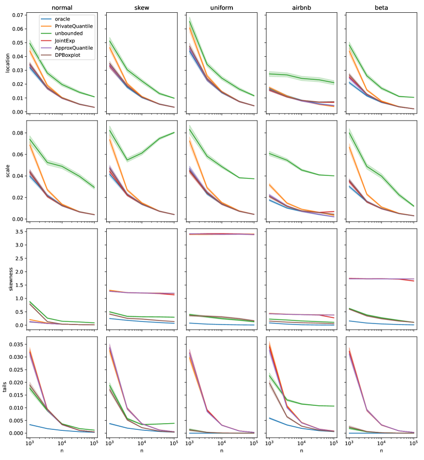
Data were generated from the five distinct distributions parametrized to have mean 0 and variance 1: normal distribution (normal), skew normal distribution (skew), uniform distribution (uniform), beta distribution (beta), and distribution of data from 2019 NY airbnb listing prices (airbnb)222These data were sampled without replacement.. The results from the beta and airbnb distributions did not convey any additional insights, and so we defer these to Appendix B.1 We considered multiple sample sizes and privacy budgets . Each scenario was simulated 1000 times. (For more details, see Appendix B.1).
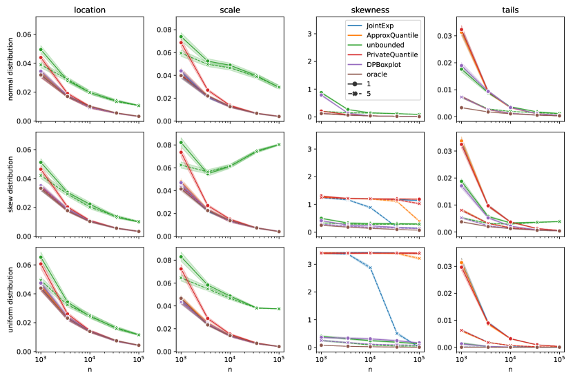
Figure 1 provides a comprehensive summary of the simulation results. Each column of figures corresponds to a distinct boxplot component, while each row pertains to a different generating distribution. The sample size is depicted along the -axis, while the average error is represented on the -axis. The line color within the figures denotes the method used to generate the boxplot and the line style corresponds to the privacy budget .
Consistent with Theorems 2, 3, and 5, the error for the DPBoxplot is converging to the oracle in all aspects under all simulated distributions with increasing sample sizes. We also observe a slower convergence in skewness and tails compared to location and scale, which is expected as distributional extremes are more difficult to estimate privately. This shows that the error between the proposed differentially private boxplot and its population counterpart is similar to that of the error between the non-private boxplot and its population counterpart. That is, the sampling error is larger than that of the error attributed to privatization.
Observe that the naive boxplots do not exhibit the same behavior. In particular, the inconsistency of the whiskers for the naive methods based on JointExp, ApproxQuantile, and PrivateQuantile leads to very poor performance in the skew metric for the skew and uniform distributions. This is due to the inconsistency of all three of these algorithms for estimating extreme quantiles. On the other hand, though it does well at estimating the extreme quantiles, the unbounded algorithm exhibits poor performance in terms of estimating scale and location, relative to the other algorithms. We observe that, in general, DPBoxplot method exhibits consistently better behavior, except notable with small sample sizes in the normal distribution. This happens because at small sample sizes, the unbounded algorithm tends to underestimate the magnitude of the minimum and maximum of the dataset, while the other algorithms overestimate this magnitude.
We also assessed the ability to compare multiple distributions through simulation, concluding that DPBoxplot also performs well under this setting. For brevity, this study is defered to Appendix B.3
6 Case study
We now conduct an exploratory data analysis via boxplots, within the framework of differential privacy. To maintain the authenticity of the case study, privacy budgets are proportionally distributed across all visualizations explored in the process of addressing each question. To elaborate, out of the total budget (), each visualization is assigned a privacy budget equal to the number of boxplots in the visualization, divided by the number of boxplots on all generated visualizations. The purpose for this allocation is to provide more budget for visualizations where the data is partitioned more times and hence sample sizes are smaller. Code for replicating these findings has been made publicly accessible .
We analyze a dataset containing Airbnb listing prices and associated metrics within New York City (NYC) in 2019 (Kaggle,, 2019). After removing listings priced above 500 US dollars (USD) and requiring minimum nights of stay fewer than 10, this dataset has observations and explanatory variables of business interest. We only consider listings priced below 500 USD, and so we set and . We address two distinct business inquiries:
Inquiry 1: Do discernible patterns emerge in Airbnb listing prices across various boroughs in New York City and differing room types?
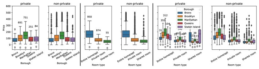
The dataset encompasses five distinct boroughs within New York City, namely Bronx, Brooklyn, Manhattan, Queens, and Staten Island, alongside three offered room types: Entire Home, Private Room, and Shared Room. We present three visualizations: boxplots of prices by borough, by room type, and a combined visualization of prices by borough and room type. These generate 5, 3, and 15 boxplots, respectively, totaling 23.
The differentially private boxplots are displayed in Figure 2, juxtaposed with their non-private counterparts. Only looking at the differentially private boxplots, Figure 2 reveals that prices predominantly lie in the bottom end of the range [0,500], with a right skew and heavy right tail observed across all boroughs and room types, except for in the Bronx, and for shared rooms. The distribution of prices in the Bronx still exhibits a right skew, but has light tails. The distribution of prices for shared rooms appears to be symmetric, with light tails. Notably, prices appear elevated for Manhattan. As expected, entire homes are priced higher than shared spaces. The right-most plot, which displays prices by both borough and room type, affirms previous observations, except shared rooms in Staten Island and the Bronx. Staten Island and the Bronx exhibits higher variability for shared rooms.
It is natural to compare the patterns observed on the differentially private boxplots to those observed in the non-private boxplots. As previously mentioned, Figure 2 juxtaposes the differentially private boxplots with the non-private boxplots. Many conclusions derived from the private visualizations persist in the non-private domain. However, there are several disparities, which are outlined are as follows: In reality, both the listing prices for shared rooms and properties in the Bronx do have a heavy, right tail. The second disparity occurs in the third plot, where the non-private plots does not indicate higher prices and variability for properties in Staten Island and the Bronx in shared rooms. These discrepancies can be explained by small sample sizes and our conservative choice of privacy budget. For instance, the number of shared room listings in Staten Island is only 9. Low sample sizes underscore potential for greater discrepancies between private and non-private boxplot representations. It may be of interest to allocate more privacy budget to visualizations generated from smaller subsets of the dataset.
Inquiry 2: Are there observable trends in Airbnb listing prices concerning minimum nights required for reservation and the types of rooms offered?
We create a new categorical variable called minimum nights, in which a listing is assigned “low” if it has less than or equal to three minimum nights, and “high” otherwise. For this inquiry, we generate two visualizations: Boxplots of prices by minimum nights, and prices by combinations of minimum nights and room offered. These visualizations require 2, and 6 boxplots, respectively, totaling 8.
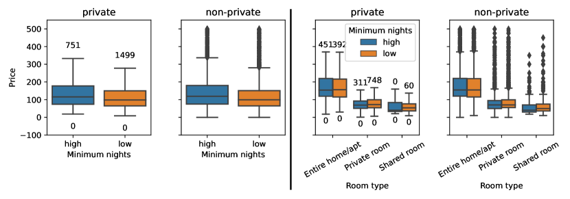
The differentially private boxplots are displayed in Figure 3, juxtaposed with their non-private counterparts. Again, we first analyze the patterns in the differentially private boxplots, and compare to those observed in the private boxplots afterward. The differentially private boxplots indicate the emergence of a phenomenon akin to Simpson’s paradox. Specifically, a preliminary examination suggests that listings requiring a higher minimum number of nights are priced more steeply than their counterparts with lower minimum requirements. However, this trend disappears when the data is divided by room type. Listings for entire rooms exhibit no significant price differential based on minimum night requirement, while private rooms slightly favor lower minimum nights in terms of price. In shared rooms the median price does not seem to be significantly different.
A comparative analysis with non-private boxplots reaffirms these observations; we observe relatively consistent patterns between the private and non-private boxplots. The primary visual disparity pertains to the positioning of the lower whiskers on the boxplots. This underscores the recognized challenge associated with differentially private estimation of extreme quantiles. However, this discrepancy does not materially impede the analytical value of our findings.
Overall, the patterns observed are generally consistent between the private and non-private boxplots. The principal disparities are attributable to sample size, a factor that we encourage practitioners to consider when conducting differentially private exploratory analyses. This case study demonstrates the potential of differentially private, exploratory data analysis and confirms the efficacy of the differentially private boxplot, in accordance with our theoretical and simulated results.
References
- Acharya et al., (2021) Acharya, J., Sun, Z., and Zhang, H. (2021). Differentially private Assouad, Fano, and Le Cam. In Feldman, V., Ligett, K., and Sabato, S., editors, Proceedings of the 32nd International Conference on Algorithmic Learning Theory, volume 132 of Proceedings of Machine Learning Research, pages 48–78. PMLR.
- Acs et al., (2012) Acs, G., Castelluccia, C., and Chen, R. (2012). Differentially private histogram publishing through lossy compression. In 2012 IEEE 12th International Conference on Data Mining, pages 1–10. IEEE.
- Alabi et al., (2022) Alabi, D., Ben-Eliezer, O., and Chaturvedi, A. (2022). Bounded space differentially private quantiles.
- Bhattacharjee et al., (2020) Bhattacharjee, K., Chen, M., and Dasgupta, A. (2020). Privacy-preserving data visualization: Reflections on the state of the art and research opportunities. Computer Graphics Forum, 39:675–692.
- Budiu et al., (2022) Budiu, M., Thaker, P., Gopalan, P., Wieder, U., and Zaharia, M. (2022). Overlook: Differentially private exploratory visualization for big data. Journal of Privacy and Confidentiality, 12.
- Dasgupta et al., (2013) Dasgupta, A., Chen, M., and Kosara, R. (2013). Measuring privacy and utility in privacy-preserving visualization. Computer Graphics Forum, 32:35–47.
- Dasgupta and Kosara, (2011) Dasgupta, A. and Kosara, R. (2011). Adaptive privacy-preserving visualization using parallel coordinates. IEEE Transactions on Visualization and Computer Graphics, 17(12):2241–2248.
- Dasgupta et al., (2019) Dasgupta, A., Kosara, R., and Chen, M. (2019). Guess me if you can: A visual uncertainty model for transparent evaluation of disclosure risks in privacy-preserving data visualization. In 2019 IEEE Symposium on Visualization for Cyber Security (VizSec), pages 1–10.
- Durfee, (2023) Durfee, D. (2023). Unbounded differentially private quantile and maximum estimation. In Oh, A., Neumann, T., Globerson, A., Saenko, K., Hardt, M., and Levine, S., editors, Advances in Neural Information Processing Systems, volume 36, pages 77691–77712. Curran Associates, Inc.
- Dwork, (2008) Dwork, C. (2008). Differential privacy: A survey of results. In International conference on theory and applications of models of computation, pages 1–19. Springer.
- Dwork et al., (2006) Dwork, C., McSherry, F., Nissim, K., and Smith, A. (2006). Calibrating noise to sensitivity in private data analysis. In Theory of Cryptography Conference, pages 265–284.
- Garrido et al., (2023) Garrido, G. M., Liu, X., Matthes, F., and Song, D. (2023). Lessons learned: Surveying the practicality of differential privacy in the industry. Proceedings on Privacy Enhancing Technologies, 2023:151–170.
- Gillenwater et al., (2021) Gillenwater, J., Joseph, M., and Kulesza, A. (2021). Differentially private quantiles. In Meila, M. and Zhang, T., editors, Proceedings of the 38th International Conference on Machine Learning, volume 139 of Proceedings of Machine Learning Research, pages 3713–3722. PMLR.
- Hay et al., (2010) Hay, M., Rastogi, V., Miklau, G., and Suciu, D. (2010). Boosting the accuracy of differentially private histograms through consistency. Proc. VLDB Endow., 3(1–2):1021–1032.
- He et al., (2016) He, X., Raval, N., and Machanavajjhala, A. (2016). A demonstration of visdpt. Proceedings of the VLDB Endowment, 9:1489–1492.
- Hongde et al., (2014) Hongde, R., Shuo, W., and Hui, L. (2014). Differential privacy data aggregation optimizing method and application to data visualization. In 2014 IEEE Workshop on Electronics, Computer and Applications, pages 54–58.
- Ji et al., (2014) Ji, Z., Lipton, Z. C., and Elkan, C. (2014). Differential privacy and machine learning: a survey and review.
- Kaggle, (2019) Kaggle (2019). New york city airbnb open data.
- Kaplan et al., (2022) Kaplan, H., Schnapp, S., and Stemmer, U. (2022). Differentially private approximate quantiles. In Chaudhuri, K., Jegelka, S., Song, L., Szepesvari, C., Niu, G., and Sabato, S., editors, Proceedings of the 39th International Conference on Machine Learning, volume 162 of Proceedings of Machine Learning Research, pages 10751–10761. PMLR.
- Kellaris and Papadopoulos, (2013) Kellaris, G. and Papadopoulos, S. (2013). Practical differential privacy via grouping and smoothing. Proceedings of the VLDB Endowment, 6(5):301–312.
- (21) Lalanne, C., Garivier, A., and Gribonval, R. (2023a). Private statistical estimation of many quantiles. In Krause, A., Brunskill, E., Cho, K., Engelhardt, B., Sabato, S., and Scarlett, J., editors, Proceedings of the 40th International Conference on Machine Learning, volume 202 of Proceedings of Machine Learning Research, pages 18399–18418. PMLR.
- (22) Lalanne, C. S., Gastaud, C., Grislain, N., Garivier, A., and Gribonval, R. (2023b). Private quantiles estimation in the presence of atoms.
- Li et al., (2010) Li, C., Hay, M., Rastogi, V., Miklau, G., and McGregor, A. (2010). Optimizing linear counting queries under differential privacy. In Proceedings of the twenty-ninth ACM SIGMOD-SIGACT-SIGART symposium on Principles of database systems, pages 123–134.
- Liu et al., (2023) Liu, W., Zhang, Y., Yang, H., and Meng, Q. (2023). A survey on differential privacy for medical data analysis. Annals of Data Science, 11(2):733–747.
- Nanayakkara et al., (2022) Nanayakkara, P., Bater, J., He, X., Hullman, J., and Rogers, J. (2022). Visualizing privacy-utility trade-offs in differentially private data releases. Proceedings on Privacy Enhancing Technologies, 2022:601–618.
- Panavas et al., (2024) Panavas, L., Crnovrsanin, T., Adams, J. L., Ullman, J., Sargavad, A., Tory, M., and Dunne, C. (2024). Investigating the visual utility of differentially private scatterplots. IEEE Transactions on Visualization and Computer Graphics, pages 1–16.
- Ramsay et al., (2024) Ramsay, K., Jagannath, A., and Chenouri, S. (2024). Differentially private multivariate medians.
- Smith, (2011) Smith, A. (2011). Privacy-preserving statistical estimation with optimal convergence rates. In Proceedings of the forty-third annual ACM symposium on Theory of computing, STOC’11. ACM.
- Tukey et al., (1977) Tukey, J. W. et al. (1977). Exploratory data analysis, volume 2. Springer.
- Tzamos and Vlatakis-Gkaragkounis, (2020) Tzamos, C. and Vlatakis-Gkaragkounis (2020). Optimal private median estimation under minimal distributional assumptions. In Larochelle, H., Ranzato, M., Hadsell, R., Balcan, M., and Lin, H., editors, Advances in Neural Information Processing Systems, volume 33, pages 3301–3311.
- Xu et al., (2013) Xu, J., Zhang, Z., Xiao, X., Yang, Y., Yu, G., and Winslett, M. (2013). Differentially private histogram publication. The VLDB journal, 22:797–822.
- Zhang et al., (2016) Zhang, D., Hay, M., Miklau, G., and O’connor, B. (2016). Challenges of visualizing differentially private data.
- Zhang et al., (2014) Zhang, X., Chen, R., Xu, J., Meng, X., and Xie, Y. (2014). Towards accurate histogram publication under differential privacy. pages 587–595. Society for Industrial and Applied Mathematics.
- Zhou et al., (2022) Zhou, J., Wang, X., Wong, J. K., Wang, H., Wang, Z., Yang, X., Yan, X., Feng, H., Qu, H., Ying, H., and Chen, W. (2022). Dpviscreator: Incorporating pattern constraints to privacy-preserving visualizations via differential privacy. IEEE Transactions on Visualization and Computer Graphics, pages 1–11.
Appendix A Technical proofs
Before presenting the proof of Theorem 2, we first prove a general sample complexity bound for quantiles. For , such that , , and , define:
One may wish to recall that , and so is still defined if .
Lemma 6.
For , if is absolutely continuous such that , then there exists universal constants such that for all such that and , all and , it holds that , with probability , provided that
| (3) |
Proof of Lemma 6.
Given that is a draw from the exponential mechanism, the result follows from an application of Corollary 7 of Ramsay et al., (2024). Corollary 7 of Ramsay et al., (2024) gives an upper bound on the sample complexity of a draw from the exponential mechanism, provided the utility function meets certain criteria. In order to apply Corollary 7 of Ramsay et al., (2024), we must show that the following function
and satisfy three conditions. First, we must show that has a maximum, which is easily seen by definition, is maximized at . The second requirement is that is -Lipschitz, which follows by assumption. Lastly, Corollary 7 of Ramsay et al., (2024) requires that is a regular function for some with , see Definition 2. It is easy to see that is regular function with . In order to apply the bound, we must compute the discrepancy function of , which is given by: A straightforward calculation yields that . Applying Corollary 7 of Ramsay et al., (2024), yields that there exists a universal constant such that with probability at least , if
Define if there exists a universal constant such that (). Next, using the Lipschitz assumption and the mean value theorem, we have that which yields the desired result. ∎
We can now prove Theorem 2.
Proof of Theorem 2.
The proof is based on an application of Lemma 6. All of the conditions of Lemma 6 are satisfied by assumption, and so it remains to lower bound . To this end, let . Using this notation, for , the definition of in conjunction with the mean value theorem yields that
Applying this bound, in conjunction with Lemma 6, yields the desired result. ∎
Next, we prove Theorem 3.
Proof of Theorem 3.
We apply Corollary 4 of (Acharya et al.,, 2021), of which a simpler version is restated below for clarity. For , let
Corollary 7 (Acharya et al., (2021)).
For all and any , let . If for all , it holds that , , and , then then .
In order to apply Corollary 7, we first define a class of Gaussians which lie in . Recall that we consider with densities which satisfy: . Let and let denote the associated quantile function. We have that for , it holds that
Taking gives that
Now, note that
which in turn implies that
Next, we have that
We must then have that , which holds by assumption. Define . We find the values of and for . Consider the values , and for =1 or , denote . Note that for any quantile , we have that . That is, the distance between the quantiles is just the difference between the means. For some , take any such that . It follows that and . Therefore, applying Corollary 7 gives that
Before proceeding with the proof of Theorem 5, we first prove that the unbounded algorithm estimates extreme quantiles consistently.
Lemma 8.
For all , such that , it holds that
-
i
if , then .
-
ii
if , then .
Proof.
First, using the fact that is an exponential random variable, we have that as . In addition, letting , the Dvoretzky–Kiefer–Wolfowitz inequality yields that . It suffices to show that as . (A symmetric argument then implies then that also, as .) We have that
for which we can write
It suffices to show that as . To this end, we have that
Now, for large , we have that
where the last inequality uses the fact that for all and . Applying this inequality yields that
as . On the other hand, for the term , we have that
as . ∎
We can now prove Theorem 5.
Proof of Theorem 5.
We first prove that the whiskers are consistent. Theorem 2 gives that and Lemma 8 gives that . Continuous mapping theorem and the fact that as yields that . The same argument applies to the upper whisker.
For the outlyingness number, first, we have that . Next, the properties of the Laplace distribution give that . Therefore, , or, . Next, using the fact that , we have that is -Lipschitz. It follows that . Next, the Dvoretzky–Kiefer–Wolfowitz inequality yields that and the fact that the whiskers are consistent implies that . The same argument can be made for the upper outlyingness number. ∎
Appendix B Simulation details and additional results
B.1 Single boxplot estimation
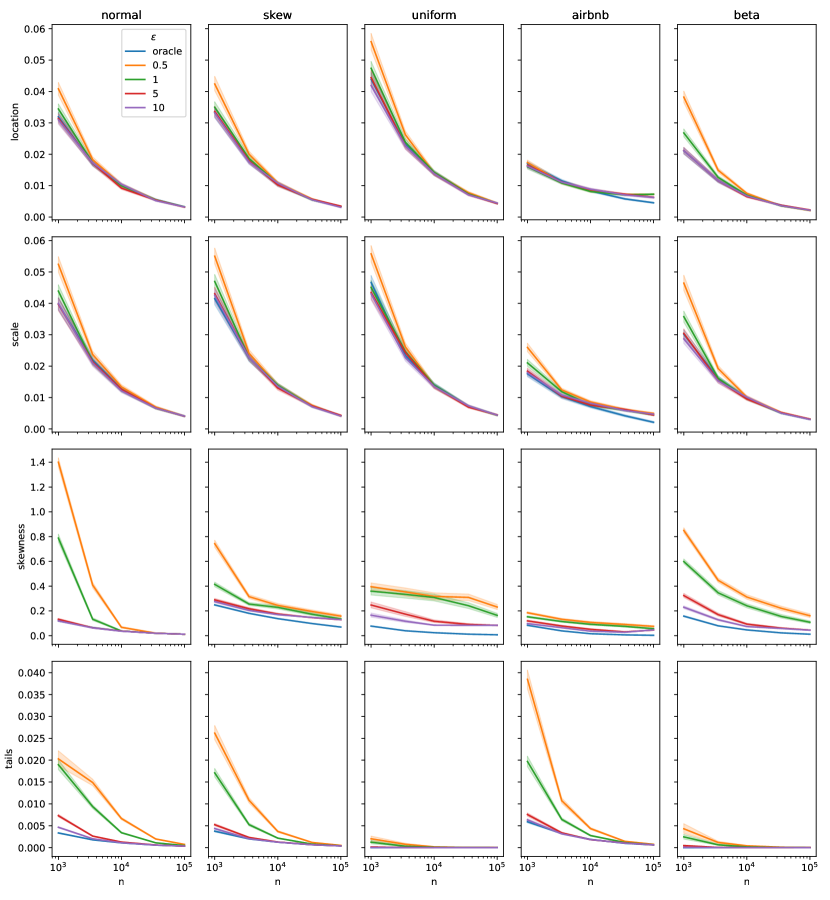
This section presents more details on the simulation study described in 5. We simulated data from five distributions, each with mean 0 and variance 1: standard normal distribution (normal), skew normal distribution with scale parameter 20 (skew), uniform distribution with interval (uniform), a normalized and mean-centered version of the beta distribution with (beta), and normalized and mean-centered empirical distribution of data from 2019 NY airbnb listing prices sampled without replacement. We considered sample sizes of and privacy budgets of . Each scenario was simulated 1000 times leading to simulated data vectors . For each generated dataset, we computed both the non-private boxplots . We also calculated differentially private boxplots using each of the methods. We then quantified boxplot distances against location, scale, skewness, and tails metrics between the differentially private boxplots and their corresponding population boxplots. We also calculated the oracle distance between the sample non-private boxplot and the population boxplot. Figures 4 and 5 give a more detailed overview of the results from this simulation study.
B.2 Parameter tuning
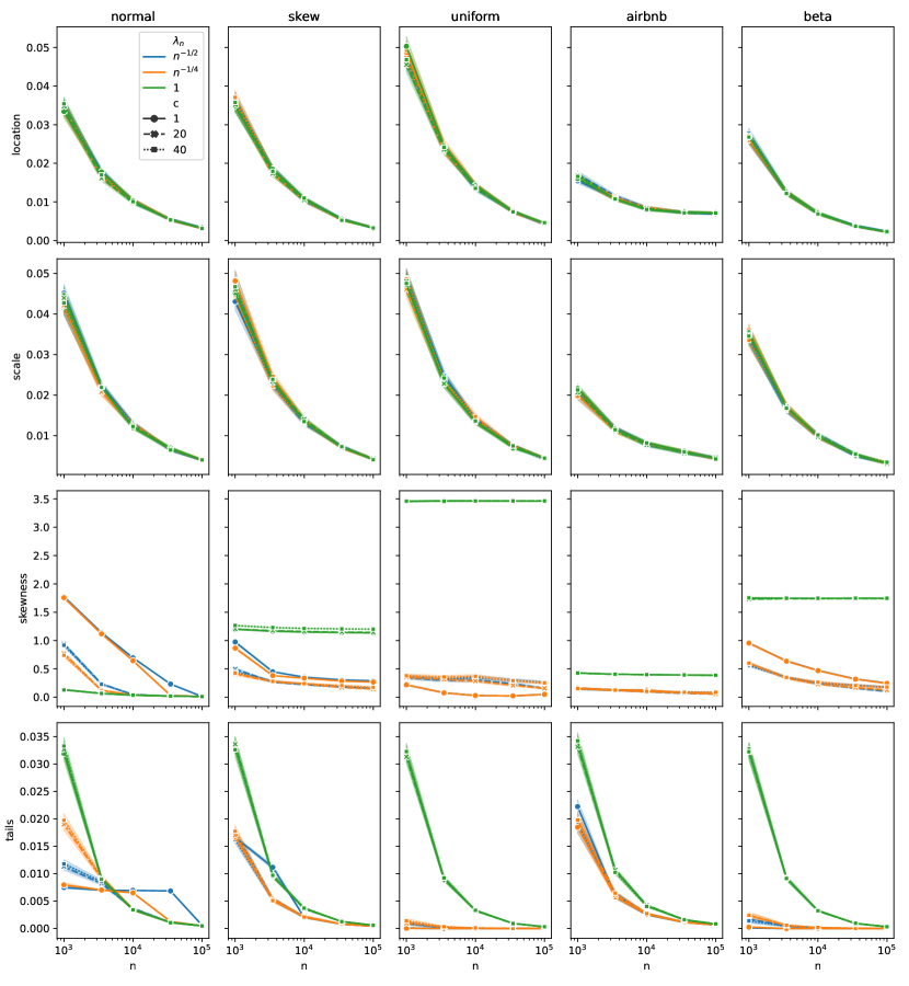
We performed simulations under similar settings as in the previous section. We varied and , fixing and estimated differentially private boxplots with DPBoxplot. . Figure 6 summarizes the results for simulated distributions (column-wise), boxplot metrics (row-wise). Variations in and in are represented with different line colors and line styles, respectively. We observe the method is not highly sensitive to the chosen parameters except for skewness and tails. Based on this observation and to account for better results in small samples we concluded that and were reasonable choices.
B.3 Multiple boxplot estimation
This section presents an extensive simulation study to assess the differentially private boxplot’s ability to describe, and facilitate comparison of multiple samples. Specifically, we analyze whether the metrics (quantified by distances on location, scale, skewness and tails as in Section 5) between differentially private boxplots across distinct datasets mirror the corresponding pairwise distances observed between their population counterparts. The similitude between two distinct differentially private boxplots is anticipated to align closely with the similitude observed between their respective population counterparts, thereby facilitating analogous visual comparisons and interpretation. For the purpose of quantifying this phenomenon, we introduce the concept of relative similitude between two differentially private boxplots as follows:
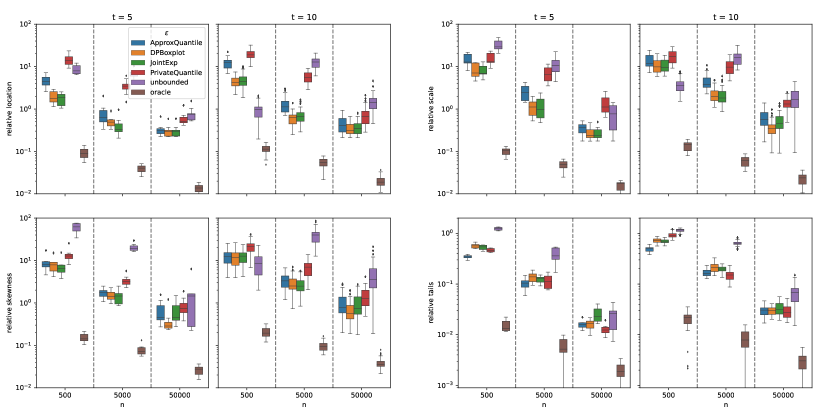
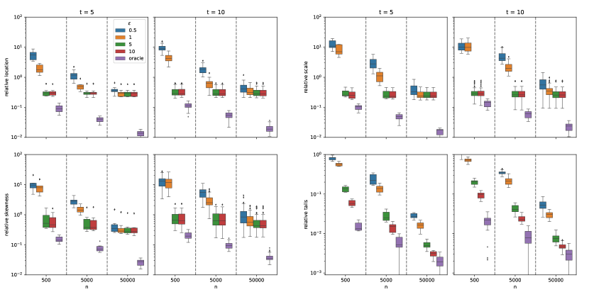
Here, distance is related to the four metrics previously described. In order to empirically validate the consistency of our proposed approach with this behavior, we conducted Monte Carlo simulations by generating datasets , and two vectors and of size sampling from uniform distributions with interval and , respectively. Each vector is size for where is chosen randomly such that . Here, plays the role of the number of treatments in an experiment. We replicated this simulation 1000 times for each combination of and leading to datasets such that . We performed this simulation generating the initial datasets using mixture of the five distributions described in the previous section such that each distribution generates the same amount of vectors on each replica. For each dataset we calculated non-private boxplots , and differentially private boxplots using each of the quantile estimation methods and for each . We then calculated pair-wise relative boxplot distances for every pair of differentially private boxplots.
Figure 7 and 8 offers a detailed overview of the results obtained from various scenarios considered. Each boxplot within these plots represents the average pairwise distances observed among all differentially private boxplots generated in a specific scenario. The x-axis on each plot denotes the sample size (). Variations in hue color correspond to different methods and different privacy budgets (), respectively. The first and last two plots in the first row correspond to relative location and relative scale, respectively. The first and last two plots in the second row correspond to relative skewness and relative outliers, respectively. For each pair of relative distance plots, the first and second visualization correspond to and , respectively. Figure 8 uses and Figure 7 shows results with DPBoxplot method.
Figure 7 shows that DPBoxplot is consistently good among different scenarions. All other methods have poor performance in at least one scenario. In Figure 8 relative distances exhibit a diminishing trend with augmented sample sizes and , consistent with expectations illustrated by the oracle boxplot. A marginal increase in the parameter leads to a slight augmentation in the relative distances, attributable to the partitioning of data into smaller subsets and consequent reduction in sample sizes; however, this impact appears to be negligible. Hence, our analysis suggests that our proposed methodology effectively maintains the visual coherence of relative similarities among diverse boxplots during the execution of multiple comparisons.
B.4 Computational requirements
All simulations were conducted on a single CPU and did not require significant computational resources. The execution time for the simulations presented in the paper did not exceed 24 hours.
Appendix C Auxiliary results
The next lemma says that JointExp is inconsistent for .
Lemma 9.
For , if there exists such that , then for any , we have that
Proof.
We have that
In this case, if , then the sample complexity is then at least .
Lemma 10.
For all , , we have that if .
Proof.
First, note that is increasing for . Now, for we can use the fact that for to get whenever . ∎
Let denote the space of Borel functions from to . For a family of functions, , define a pseudometric on , , where .
Definition 2 (Ramsay et al., (2024)).
We say that is -regular if there exists a class of functions such that is -Lipschitz with respect to the -pseudometric uniformly in , i.e., for all
Appendix D Broader impacts
Our proposed methodology inherits the extensive implications, both beneficial and detrimental, of differential privacy. Differential privacy significantly enhances data confidentiality by introducing noise into datasets, which complicates the ability to link specific data points to individual identities. This greatly enhances the privacy awarded to individuals whose information is contained in such datasets. However, this method is not without its drawbacks. The primary challenge lies in the trade-off between privacy protection and data accuracy. The introduction of noise, while safeguarding privacy, may distort the data, potentially yielding inaccurate insights or conclusions. Such inaccuracies are especially problematic in contexts requiring high precision, such as policy development or clinical research, where exact data is crucial.