Quantum encoder for fixed Hamming-weight subspaces

Abstract

We present an exact $n$-qubit computational-basis amplitude encoder of real- or complex-valued data vectors of $d=\binom{n}{k}$ components into a subspace of fixed Hamming weight $k$. This represents a polynomial space compression. The circuit is optimal in that it expresses an arbitrary data vector using only $d-1$ (controlled) Reconfigurable Beam Splitter (RBS) gates and is constructed by an efficient classical algorithm that sequentially generates all bitstrings of weight $k$ and identifies all gate parameters. An explicit compilation into CNOTs and single-qubit gates is presented, with the total CNOT-gate count of $\mathcal{O}(k\,d)$ provided in analytical form. In addition, we show how to load data in the binary basis by sequentially stacking encoders of different Hamming weights using $\mathcal{O}(d\,\log(d))$ CNOT gates. Moreover, using generalized RBS gates that mix states of different Hamming weights, we extend the construction to efficiently encode arbitrary sparse vectors. Finally, we perform an experimental proof-of-principle demonstration of our scheme on a commercial trapped-ion quantum computer. We successfully upload a $q$-Gaussian probability distribution in the non-log-concave regime with $n=6$ and $k=2$. We also showcase how the effect of hardware noise can be alleviated by quantum error mitigation. Our results constitute a versatile framework for quantum data compression with various potential applications in fields such as quantum chemistry, quantum machine learning, and constrained combinatorial optimizations.

I Introduction

Amplitude encoding schemes in the basis of Hamming-weight-$k$ (HW-$k$) states of $n$ qubits correspond to an interesting regime of polynomial space compression $n\in\mathcal{O}\big{(}k\,d^{1/k}\big{)}$ for data vectors of size $d$ [1, 2, 3, 4]. They are the middle-ground between two distinct encoding scenarios. On one end, there is an amplitude encoding scheme of zero compression that loads data in the unary basis [5, 6, 7, 8, 9]. On the other end, there are techniques to load amplitudes in binary basis, which provides exponential compression [10, 11, 12, 13, 14, 15, 16, 17, 18], but requires a number of two-qubit gates that is exponential in $n$ [19, 20, 21, 22]. Moreover, HW-$k$ encoders have the additional benefit of being the natural subspace for applications in fields such as quantum chemistry, due to the particle-preserving nature of typical Hamiltonians [1, 23, 2, 24, 25]. They have also been used in the context of quantum machine learning [6, 7, 8, 3, 26, 4] and quantum finance [5, 9, 27, 28]. When used as variational circuits, they take advantage of the reduced subspace to mitigate the barren plateau problem [29, 28, 26].

However, current implementations of HW-$k$ encoders present some drawbacks in practice. For instance, Refs. [8, 3] use the aforementioned unary-basis encoders as subroutines for their schemes. While allowing for the generalization to HW $k>1$ using only two-qubit Givens rotations, these encoders either require the orthogonalization of the input data [7] or require solving non-linear systems of $\binom{n}{k}-1$ equations to compute the rotation angles [3]. Here we address these classical overheads while still performing an exact encoding.

We present an exact, ancilla-free amplitude encoder for real and complex data in HW-$k$ subspaces. We detail a classical algorithm that, given an initial bitstring of Hamming weight $k$ and a data vector of size $d$, outputs instructions for a sequence of (controlled) Givens rotations and their respective angles in hyperspherical coordinates of the data vector, hence efficient to compute. An explicit compilation into CNOTs and single-qubit gates is presented, with the total CNOT-gate count of $\mathcal{O}(k\,d)$ provided in analytical form. Moreover, our Hamming-weights-$k$ encoder can be used as a subroutine to power more complex algorithms. For instance, by combining all Hamming weights $k\leq n$ we obtain a binary encoder using $\mathcal{O}(d\,\log(d))$ CNOT gates. Using a generalized RBS gate capable of mixing states with different Hamming weights, we extend our methods and derive a procedure to load data in the paradigm of classical sparse-access model. Moreover, we deploy a proof-of-concept instance on the Aria-1 ion-trap quantum processor from IonQ [30], uploading a $q$-Gaussian probability distribution. The experimental results are further enhanced using an well-known error mitigation technique called Clifford Data Regression [31, 32].

The paper is structured as follows. In Sec. II we introduce the gates used in our algorithm. Then, we present our framework for HW-$k$ encoders in Sec. III. Secs. IV and V, respectively, expand on the sparse and binary encoders using the fixed HW-$k$ encoder as a subroutine. In Sec. VI, we show the deployment of our HW-$k$ encoder on a quantum hardware, and we conclude in Sec. VII.

II Preliminaries

Let $b\in\{0,1\}^{\otimes n}$ be a bitstring of length $n$ and Hamming weight $\absolutevalue{b}$. In this section, we introduce the building blocks for our encoders, namely gates that superpose two arbitrary states $\ket{b}$ and $\ket{b^{\prime}}$ with tunable amplitudes. A gate that increases the Hamming weight by $1$ acting on a single qubit on the $\ket{0}$ state is the $R_{y}(\theta)\coloneqq e^{-i\theta Y}$ gate ($Y$ being the Pauli-$Y$ operator), since

$$R_{y}(\theta)\ket{0}=\cos\theta\ket{0}+\sin\theta\ket{1}\,.$$ (1)

Another gate of interest is one that creates a superposition between two bitstrings $\ket{b}$ and $\ket{b^{\prime}}$ of equal Hamming-weight. More precisely, denoting by $\mathcolor{blue}{in}$ a bit that has value $1$ in $b$ and $0$ in $b^{\prime}$ and by $\mathcolor{teal}{out}$ a bit that has a $0$ in $b$ and a $1$ in $b^{\prime}$, the two-qubit gate

$$R^{\mathcolor{blue}{in}}_{\mathcolor{teal}{out}}(\theta,\phi)\coloneqq\begin{bmatrix}1&&&\\ &e^{i\phi}\cos\theta&e^{-i\phi}\sin\theta&\\ &-e^{i\phi}\sin\theta&e^{-i\phi}\cos\theta&\\ &&&1\end{bmatrix}$$ (2)

acting on qubits $\mathcolor{blue}{in}$ and $\mathcolor{teal}{out}$ superposes $\ket{b}$ and $\ket{b^{\prime}}$ with tunable amplitudes (empty entries represent zeros). This gate reduces to the well-known Reconfigurable Beam Splitter (RBS) gate when $\phi=0$ . In this case, we denote $R^{\mathcolor{blue}{in}}_{\mathcolor{teal}{out}}(\theta,\phi=0)$ as $R^{\mathcolor{blue}{in}}_{\mathcolor{teal}{out}}(\theta)$. In Fig 1, we present two possible compilations of this complex RBS gate into CNOTs, $R_{y}(\theta)$, and $R_{z}(\phi)\coloneqq e^{-i\phi Z}$ gates.

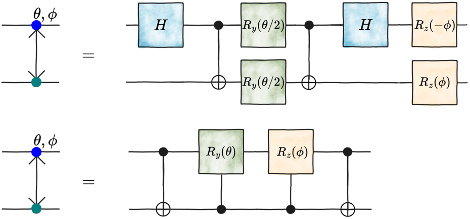
Figure 1: Possible compilations of the complex RBS gate. Decompositions of $R^{\mathcolor{blue}{in}}_{\mathcolor{teal}{out}}(\theta,\phi)$ into CNOT and single-qubit rotation gates. Colors are used to indicate the input (blue) and output (green) qubits. (Top) Complex RBS as two CNOTs and single-qubit gates; (Bottom) Complex RBS as two CNOTs and a controlled-$SU(2)$ gate. The product $R_{y}(\theta)\,R_{z}(\phi)$ can be written as a single $SU(2)$ rotation $R_{w}(\lambda):=e^{i\lambda W}$, where $\lambda(\theta,\phi)=\arccos(\cos\theta\cos\phi)$ and $W(\theta,\phi)=\frac{1}{\sin\lambda(\theta,\phi)}(-\sin\theta\sin\phi\,X+\sin\theta\cos\phi\,Y+\cos\theta\sin\phi\,Z)$. This gate reduces to the RBS gate when $\phi=0$.

Definition II.1 below generalizes the gate in Eq. (2), allowing the mixing of two states $\ket{b}$ and $\ket{b^{\prime}}$ with possibly different Hamming-weights $k$ and $k^{\prime}$.

Definition II.1 (Generalized complex RBS gate (gRBS)).

Let $n\geq 2$ be an integer, and $b,\,b^{\prime}$ be bitstrings such that $\absolutevalue{b}=k$ and $\absolutevalue{b^{\prime}}=k^{\prime}$. Let $\mathcal{I}$ and $\mathcal{I}^{\prime}$ be the sets of indices where $b$ and $b^{\prime}$ have an $1$, respectively. Define the set indexing input qubits by $\{\mathcolor{blue}{in_{1},\ldots,in_{m}}\}:=\mathcal{I}\setminus\mathcal{I}^{\prime}$, the set indexing output qubits $\{\mathcolor{teal}{out_{1},\ldots,out_{m^{\prime}}}\}:=\mathcal{I}^{\prime}\setminus\mathcal{I}$, and the set indexing control qubits $\{\mathcolor{violet}{ctrl_{1},\ldots,ctrl_{\ell}}\}\coloneqq\mathcal{I}\cap\mathcal{I}^{\prime}$, where $m$, $m^{\prime}$, and $\ell$ are their cardinalities. Then, the generalized complex RBS gate $R^{\mathcolor{blue}{in_{1},\ldots,in_{m}}}_{\mathcolor{teal}{out_{1},\ldots,out_{m^{\prime}}}}(\theta,\phi)$ is an $(m+m^{\prime})$-qubit gate acting like

$$R^{\mathcolor{blue}{in_{1},\ldots,in_{m}}}_{\mathcolor{teal}{out_{1},\ldots,out_{m^{\prime}}}}(\theta,\phi)\ket{b}=\mathcolor{blue}{e^{i\phi}\cos\theta}\ket{b}+\mathcolor{teal}{e^{-i\phi}\sin\theta}\ket{b^{\prime}}\,.$$ (3)

Moreover, whenever acting on a superposition state $\ket{\psi}$ of $n$ qubits containing $\ket{b}$, the $\ell$-controlled gate $c_{\mathcolor{violet}{ctrl_{1},\ldots,ctrl_{\ell}}}R^{\mathcolor{blue}{in_{1},\ldots,in_{m}}}_{\mathcolor{teal}{out_{1},\ldots,out_{m^{\prime}}}}(\theta,\phi)$ only mixes $\ket{b}$ and $\ket{b^{\prime}}$ as in Eq. (3), as long as $\ket{b}$ is the only state in $\ket{\psi}$ having ones at positions $\{\mathcolor{violet}{ctrl_{1},\ldots,ctrl_{\ell}}\}$.

The matrix form of $R^{\mathcolor{blue}{in_{1},\ldots,in_{m}}}_{\mathcolor{teal}{out_{1},\ldots,out_{m^{\prime}}}}(\theta,\phi)$ reads

$$R^{\mathcolor{blue}{in_{1},\ldots,in_{m}}}_{\mathcolor{teal}{out_{1},\ldots,out_{m^{\prime}}}}(\theta,\phi)\!\!\coloneqq\!\!\begin{bmatrix}\mathds{1}&&&&\\ &e^{i\phi}\cos\theta&&e^{-i\phi}\sin\theta&\\ &&\mathds{1}^{\prime}&&\\ &-e^{i\phi}\sin\theta&&e^{-i\phi}\cos\theta&\\ &&&&\mathds{1}\\ \end{bmatrix}\,,$$ (4)

where $\mathds{1}$ and $\mathds{1}^{\prime}$ are identity matrices of size $2^{m}-1$ and $2^{m}(2^{m^{\prime}}-2)$, respectively.

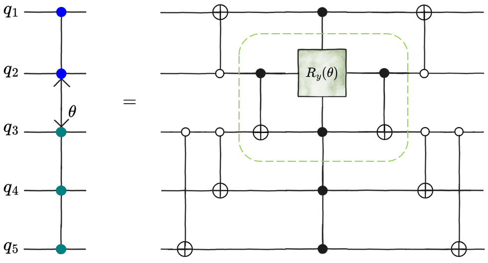
Figure 2: Possible compilation of the gRBS gate. An illustration of the $(m+m^{\prime})$-qubit gRBS gate (3) for $m=2,m^{\prime}=3$, namely $R^{\mathcolor{blue}{1,2}}_{\mathcolor{teal}{3,4,5}}(\theta)$. We chose the compilation in Fig. 1 (Bottom) with $\phi=0$ (highlighted with a green dashed box) to draw a simpler circuit, but arbitrary $\phi$ or the compilation in Fig. 1 (Top) follow similarly by replacing the box by the corresponding circuit. Colors are used to indicate input (blue) and output (green) qubits. Controlled-gRBS gates can be built by controlling directly on the rotation gate in the middle.

Remark II.2 (gRBS properties).

Let $R^{\mathcolor{blue}{in_{1},\ldots,in_{m}}}_{\mathcolor{teal}{out_{1},\ldots,out_{m^{\prime}}}}(\theta,\phi)$ be the generalized complex RBS gate as in Definition II.1. Then

1. for $m=m^{\prime}$, the gate is HW-preserving;

2. for $m\neq m^{\prime}$, the gate is HW-mixing.

In particular, for $m=m^{\prime}=1$ it reduces to Eq. (2).

In App. A we discuss the number of CNOTs needed to compile each of these gates (see Lemma A.2 for the derivation and Table 1 for a summary).

III Hamming-weight-$k$ encoders

We start this section by defining generic amplitude encoders and the concept of parameter optimality. Next, we present our Hamming-weight-$k$ encoder.

III.1 Amplitude encoders

Here we briefly define amplitude encoders with respect to an arbitrary set of computational basis states. It will be convenient to distinguish explicitly between a real-valued data vector $\vec{x}\in\mathbb{R}^{d}$ and a complex-valued one $\vec{x}\in\mathbb{C}^{d}$, since the basic quantum gates will be distinct in each case. We focus on vectors without loss of generality, given that more general formats (e.g., matrix) can be vectorized. Hereafter, we use the shorthand notation $[d]\coloneqq\{1,2,\ldots,d\}$.

Definition III.1 (Amplitude encoder).

Let $\vec{x}$ be a given $d$-dimensional (classical) data vector, $||\vec{x}||:=\sqrt{\sum_{i=1}^{d}|x_{i}|^{2}}$ be its $\ell_{2}$-norm, and $B\coloneqq\{b_{i}\in\{0,1\}^{\otimes n}\}_{i\in[d]}$ be an arbitrary set of $d$ bitstrings of length $n$ with $n\geq\log_{2}(d)$. An amplitude encoder in the basis $B$ is an $n$-qubit parameterized quantum circuit $\operatorname{Load}_{B}(\vec{x})$ that prepares a quantum state with the (normalized) vector entries $x_{i}$ as quantum amplitudes associated with the computational state $\ket{b_{i}}$, namely

$$\operatorname{Load}_{B}(\vec{x})\,\ket{0}^{\otimes n}\coloneqq\frac{1}{||\vec{x}||}\,\sum_{i=1}^{d}\,x_{i}\,\ket{b_{i}}.$$ (5)

Due to the $\ell_{2}$ normalization, we effectively encode the normalized vector $\frac{\vec{x}}{||\vec{x}||}$, which resides in the unit ($d-1$)-sphere for $\vec{x}\in\mathbb{R}^{d}$ or ($2d-1$)-sphere for $\vec{x}\in\mathbb{C}^{d}$. For an arbitrary data vector this requires exactly $d-1$ and $2d-1$ real parameters, respectively, which motivates the following definition of a parameter-optimal encoder.

Definition III.2 (Parameter-optimal amplitude encoder).

An amplitude encoder $\operatorname{Load}_{B}(\vec{x})$ as defined in Def. III.1 is parameter-optimal if it uses exactly $d-1$ gate parameters for $\vec{x}\in\mathbb{R}^{d}$ or $2d-1$ gate parameters for $\vec{x}\in\mathbb{C}^{d}$.

Ideally, one would like to explore the entire Hilbert space accessible on $n$ qubits to encode $\vec{x}$ with exponential space compression in the basis $B_{\text{binary}}=\{0,1\}^{\otimes n}$ with $n=\lceil\log_{2}(d)\rceil$. However, for arbitrary input data, the corresponding quantum circuit is known to have exponential gate complexity [22]. Efficient quantum data loaders using $\order{d}$ two-qubit gates are known in the unary basis $B_{1}=\big{\{}b_{i}\in\{0,1\}^{\otimes n}:\absolutevalue{b_{i}}=1\big{\}}_{i\in[d]}$ [5, 6, 7, 8, 9], but they require linearly many qubits ($n=d$) and hence do not offer any space compression.

In the following Section we are interested in amplitude encoding in the basis of Hamming-weight $k$ states,

$$B_{k}\coloneqq\big{\{}b_{i}\in\{0,1\}^{\otimes n}:\absolutevalue{b_{i}}=k\big{\}}_{i\in[d]}$$ (6)

with $k\in[n]$ and $d=\binom{n}{k}$. The associated Hamming-weight preserving amplitude encoder $\operatorname{Load}_{B_{k}}(\vec{x})$ corresponds to the intermediate regime of polynomial space compression $n\in\mathcal{O}\big{(}k\,d^{1/k}\big{)}$. Notice that the binary basis can in principle be constructed by combining HW-$k$ basis for all $k$, i.e., $\bigcup_{k=0}^{n}B_{k}=B_{\text{binary}}$ (see Sec. V for a binary encoder exploring this feature).

III.2 HW-$k$ amplitude encoder

In this Section we introduce our amplitude encoder $\operatorname{Load}_{B_{k}}(\vec{x})$ in the basis (6) of HW-$k$ states. Hereafter $\vec{x}$ is assumed to have dimension $d=\binom{n}{k}$. The resulting quantum circuit uses as basic ingredients the Hamming-weight-preserving gates introduced in Sec. II. The circuit architecture is decided by a classical algorithm that generates a list $\{b_{j}\}_{j\in[d]}$ of all HW-$k$ bitstrings in a particular order that minimizes the number of bit flips between $b_{i}$ and $b_{i+1}$, while identifying at each step the gate needed to superpose the corresponding states $\ket{b_{i}}$ and $\ket{b_{i+1}}$ with the correct amplitudes. For $k=1$ the resulting circuit recovers precisely the unary encoder in the diagonal architecture studied in [34].

The general procedure to construct the circuit, given by Alg. 3 in the case of $\vec{x}\in\mathbb{R}^{d}$ or by Alg. 4 in the case of $\vec{x}\in\mathbb{C}^{d}$, has four independent parts that can be summarized as follows:

The first step generates all Hamming-weight-$k$ bitstrings that will carry the amplitudes $\frac{x_{j}}{\norm{\vec{x}}}$. Here, we use Ehrlich’s algorithm [35] to create them without repetition by flipping only a pair of bits at each step. The algorithm starts from an initially marked bitstring and follows an iterative procedure, detailed in Alg.1, of marking bits yet to be exchanged, and swapping the rightmost marked bit – the “pivot” – with a bit selected according to the pivot value. This way, starting from the bitstring $1^{k}0^{n-k}$ with the $1$ bits initially marked, we generate all HW-$k$ bitstrings after exactly $\binom{n}{k}-1$ iterations.

1 NextBS(b, marked)

2 while $marked\neq\emptyset$ do

3       $m\leftarrow$ $\max(marked)$ $\triangleright$ index of rightmost marked bit

4       if $b(m)=0$ then

5             $\ell\leftarrow$ index of nearest $1$ to the right of $m$

6            

7      else

8             $\ell\leftarrow$ index of farthest $0$ to the right of $m$, without passing another $1$

9            

10      $b\leftarrow b$ with $b(m)$ and $b(\ell)$ exchanged

11       $j\leftarrow$ starting index of the last sequence of equal bits

12       $marked\leftarrow marked\setminus\{m\}$ $\triangleright$ unmark bit $b(m)$

13       $newmarks\leftarrow\{m+1,\ldots,j-1\}$

14       $marked\leftarrow marked\cup newmarks$ $\triangleright$ mark all bits between $b(m)$ and $b(j)$

15      

return $\{b,\,marked\}$

Algorithm 1 Find next HW-$k$ bitstring

It is important to note that Alg. 1 generates a sequence of bitstrings in a particular order that we shall refer to as Ehrlich ordering (see e.g. Tab. 2 in App. B for an example). Thus, if one is required to encode an amplitude $\frac{x_{j}}{||\vec{x}||}$ in a specific state $\ket{b_{j}}$, the input data vector $\vec{x}$ must be reordered beforehand to the same Ehrlich ordering. For now we assume that $\vec{x}$ is given in the correct ordering. When that is not the case, one can use instead the sparse-access model algorithm discussed in Sec. IV.

Once all the HW-$k$ bitstrings are generated, the RBS gate parameters can be computed using Alg. 2. For any pair of bitstrings $b_{j}$ and $b_{j+1}$, Alg. 2 determines the precise control, input, and output qubits in which to act with the corresponding controlled-RBS gate $c_{\mathcolor{violet}{ctrl}}R^{\mathcolor{blue}{in}}_{\mathcolor{teal}{out}}(\theta_{j},\phi_{j})$ (see Def. II.1) to create the superposition $e^{i\phi_{j}}\cos\theta_{j}\ket{b_{j}}+e^{-i\phi_{j}}\sin\theta_{j}\ket{b_{j+1}}$ without affecting the amplitudes previously encoded in $\ket{b_{i}}$ with $i<j$. The angles $\theta_{j},\phi_{j}$ are coordinates of the vector $\frac{\vec{x}}{||\vec{x}||}$ on the sphere and will depend on whether $\vec{x}\in\mathbb{R}^{d}$ or $\vec{x}\in\mathbb{C}^{d}$ (see Eqs. III.2.1 and III.2.2 below). More precisely, the $1$’s that remain unchanged between bitstrings $b_{j}$ and $b_{j+1}$ correspond to the control qubits, while the bits that were $1(0)$ in $b_{j}$ and became $0(1)$ in $b_{j+1}$ are associated with the input (output) of the RBS gate.

A priori, this procedure would insert a controlled-RBS gate with exactly $k-1$ controls at each step. However, some of these controls can be removed during the initial steps since the corresponding control qubits are in state $\ket{1}$ and they have not yet been superposed with another. The variable untouched in Alg. 2 keeps track of these redundant control qubits and removes them from the list of controls returned by the algorithm. As a result of this optimization, instead of the naive count of $\binom{n}{k}-1$ cRBS gates with $k-1$ controls each, the circuit output by Alg. 3 actually consists of $\binom{n-(k-\ell)}{\ell+1}$ cRBS gates having $\ell$ controls each, with $\ell=0,\ldots,k-1$ (namely, $\ell=0$ corresponds to removing all the controls and $\ell=k-1$ to no removal). This will be important to compute the total CNOT cost of the circuit. Notice that the total number of parameterized gates $\sum_{\ell=0}^{k-1}\binom{n-(k-\ell)}{\ell+1}=\binom{n}{k}-1$ remains the same. Denoting by $C_{\ell}$ the CNOT cost of a single $\ell$-controlled-$R^{\mathcolor{blue}{in}}_{\mathcolor{teal}{out}}(\theta,\phi)$ gate, the total CNOT count of the HW-$k$ encoder $\operatorname{Load}_{B_{k}}(\vec{x})$ generated by Alg. 3 is

$$\#\text{ CNOTs} =\sum_{\ell=0}^{k-1}\binom{n-(k-\ell)}{\ell+1}\,C_{\ell}\leq\left[\binom{n}{k}-1\right]\,C_{k-1}\,.$$ (7)

The inequality above is the naive count without simplifying initial controls. This will be the exact gate count in situations where the simplification is not possible because the initial state already contains a superposition, such as the binary encoder to be discussed in Sec. V. The precise values of $C_{\ell}$ depend on the compilation (see App. A for details) and also differ between $\phi=0$ and $\phi\neq 0$ (i.e., for real- and complex-valued data). Explicit expressions for each of these cases will be presented below in Lemmas III.3 and III.4. The specific initial bitstring $1^{k}0^{n-k}$ for the Ehrlich’s algorithm naturally reduces the CNOT-gate cost by removing controls with Alg. 3. Furthermore, it groups together controls of cRBS gates. This opens the possibility of using one clean ancillary qubit to implement all grouped controls at the same time, thus further reducing the total amount of CNOT gates in the circuit. Later, we will present CNOT-gate counts for the ancilla-free implementation only.

It is important to mention that for Hamming weight $k>n/2$ one can avoid the costly implementation of ($k-1$)-controlled-RBS gates that would arise from the above procedure by exploring the fact that every HW-$k$ bitstring is the negation of another of HW-($n-k$). Therefore, a more efficient circuit can be built by copying the architecture of a HW-($n-k$) encoder circuit with the initial state negated and controlled-RBS gates replaced by anti-controlled-RBSs.

1 GateParams($b,b^{\prime},untouched$)

2 $\mathcal{I}\leftarrow$ list of indices where $b$ has an $1$

3 $\mathcal{I}^{\prime}\leftarrow$ list of indices where $b^{\prime}$ has an $1$

4 $\mathcolor{violet}{ctrl}\leftarrow\mathcal{I}\cap\mathcal{I}^{\prime}$

5 $\mathcolor{blue}{in}\leftarrow\mathcal{I}\setminus\mathcolor{violet}{ctrl}$

6 $\mathcolor{teal}{out}\leftarrow\mathcal{I}^{\prime}\setminus\mathcolor{violet}{ctrl}$

7 $untouched\leftarrow untouched\setminus\{\mathcolor{blue}{in},\mathcolor{teal}{out}\}$

8 $\mathcolor{violet}{ctrl}\leftarrow\mathcolor{violet}{ctrl}\setminus untouched$

return $\{\mathcolor{blue}{in},\,\mathcolor{teal}{out},\,\mathcolor{violet}{ctrl},untouched\}$

Algorithm 2 Gate parameters from $b$ and $b^{\prime}$

There are multiple ways of obtaining the angles of the RBS gates depending of the choice of coordinate system on the sphere, as well as whether the input data vector is real or complex. The next two sections cover both the real and complex encoding using the hyperspherical coordinates system.

1 HWkEncoder(n, k, $\vec{x}$) $\triangleright$ assuming $d\leq\binom{n}{k}$

2 $\mathcal{C}\leftarrow{\rm Circuit}(n)$

3 for $i\leftarrow 1\;\textnormal{{to}}\;k$ do

4       $\mathcal{C}.\text{add}\big{(}X(n-i+1)\big{)}$

5      

6$b1\leftarrow 1^{k}0^{n-k}$ $\triangleright$ initial bitstring

7 $marked\leftarrow\{1,\ldots,k\}$ $\triangleright$ indices of marked bits

8 $untouched\leftarrow\{n-k+1,\ldots,n\}$ $\triangleright$ indices of ones that have never been flipped

9 for $i\leftarrow 1\;\textnormal{{to}}\;d-1$ do

10       $\{b2,marked\}\leftarrow\textnormal{{\text{\sc{NextBS}}}}(b1,marked)$

11       $\{\mathcolor{blue}{in},\mathcolor{teal}{out},\mathcolor{violet}{ctrl},untouched\}\leftarrow\textnormal{{\text{\sc{GateParams}}}}(b1,b2,untouched)$

12       $\theta_{i}$ is given by Eq. (III.2.1)

13       $\mathcal{C}.\text{add}\big{(}\text{RBS}(\mathcolor{blue}{in},\mathcolor{teal}{out},\theta_{i}).\text{controlled\_by}(\mathcolor{violet}{ctrl})\big{)}$

14       $b1\leftarrow b2$

15      

return $\mathcal{C}$

Algorithm 3 HW-$k$ encoder for dense $\vec{x}\in\mathbb{R}^{d}$

III.2.1 Dense real-valued data

For $\vec{x}\in\mathbb{R}^{d}$, the $d-1$ angles of the $c_{\mathcolor{violet}{ctrl}}R^{\mathcolor{blue}{in}}_{\mathcolor{teal}{out}}(\theta_{j})$ gates used to build the circuit in Alg. 3 are

$$\theta_{i} \coloneqq\operatorname{atan2}\left(\sqrt{\sum_{j=i+1}^{d}x_{j}^{2}},\,x_{i}\right),\quad i\in[d-2]$$

$$\theta_{d-1} \coloneqq\operatorname{atan2}\big{(}x_{d},\,x_{d-1}\big{)},$$ (8)

where the two-argument arctangent function $-\pi<\operatorname{atan2}(y,x)\leq\pi$ is the principal value of $\text{arg}(x+i\,y)$. These are the hyperspherical coordinates of the normalized vector $\frac{\vec{x}}{\norm{\vec{x}}}\in\mathbb{S}^{d-1}$, namely

$$x_{1} =\norm{\vec{x}}\cos(\theta_{1})$$

$$x_{2} =\norm{\vec{x}}\sin(\theta_{1})\cos(\theta_{2})$$

$$\,\,\,\vdots$$ (9)

$$x_{d-1} =\norm{\vec{x}}\sin(\theta_{1})\cdots\sin(\theta_{d-2})\cos(\theta_{d-1})$$

$$x_{d} =\norm{\vec{x}}\sin(\theta_{1})\cdots\sin(\theta_{d-2})\sin(\theta_{d-1})\,.$$

The resulting quantum circuit for $k=2$ for $n=6$ qubits is illustrated in Fig. 3. An explicit step-by-step execution of Alg. 3 for this example is presented in Tab. 2 in App. B. The following Lemma provides the total CNOT count to implement $\operatorname{Load}_{B_{k}}(\vec{x})$ using Alg. 3.

Lemma III.3 (Total CNOT cost of $\operatorname{Load}_{B_{k}}(\vec{x})$ for $\vec{x}\in\mathbb{R}^{d}$).

Let $n\geq 2$ and $k\in[1,n/2]$ be integers, $d=\binom{n}{k}$, and $\vec{x}\in\mathbb{R}^{d}$. The HW-$k$ encoder $\operatorname{Load}_{B_{k}}(\vec{x})$ generated by Alg. 3 can be implemented using a number $\mathcal{O}(k\,d)$ of CNOT gates, namely

$$\begin{cases}2(n-1),&k=1\\ (n-2)(3n-1),&k=2\\ \frac{1}{3}(n-3)(5n^{2}-6n-2),&k=3\\ \frac{1}{12}(n-4)(13n^{3}-58n^{2}+79n-42),&k=4\\ \frac{1}{12}\sum_{\ell=1}^{4}a_{\ell}(n-k)^{\ell}+b_{\ell}&k\geq 5\end{cases}$$ (10)

with $a_{1}=178,a_{2}=239,a_{3}=98,a_{4}=13$, and $b_{\ell}\leq\sum_{\ell=5}^{k-1}\binom{n-(k-\ell)}{\ell+1}\big{(}16\ell-6\big{)}$.

Proof.

The total CNOT count is given by the general expression (7), where $C_{\ell}$ is the cost of compiling a single $\ell$-controlled-$R^{\mathcolor{blue}{in}}_{\mathcolor{teal}{out}}(\theta)$ gate. This is computed in Lemma A.2 and summarized in Tab. 1 in App. A. Plugging in the expression immediately leads to Eq. (10). ∎

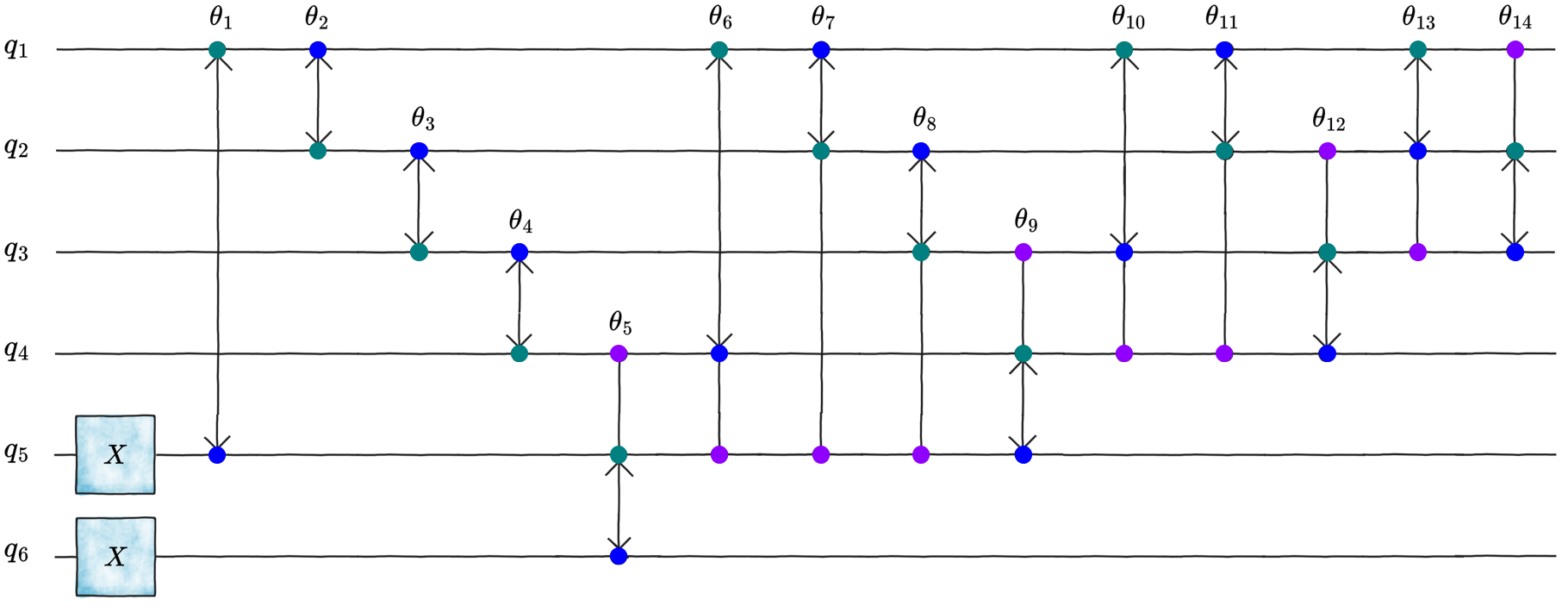
Figure 3: Hamming-weight $k=2$ quantum encoder. Circuit generated by Alg. 3 with $n=6$ (see Tab. 2 for details). Colors are used to indicate input (blue), output (green), and control (violet) qubits of each cRBS gate and angles are computed by Eq. (III.2.1).

III.2.2 Dense complex-valued data

1 HWkEncoder(n, k, $\vec{x}$) $\triangleright$ assuming $d\leq\binom{n}{k}$

2 $\mathcal{C}\leftarrow{\rm Circuit}(n)$

3 for $i\leftarrow 1\;\textnormal{{to}}\;k$ do

4       $\mathcal{C}.\text{add}\big{(}X(n-i+1)\big{)}$

5      

6$b1\leftarrow 1^{k}0^{n-k}$ $\triangleright$ initial bitstring

7 $marked\leftarrow\{1,\ldots,k\}$ $\triangleright$ indices of marked bits

8 $untouched\leftarrow\{n-k+1,\ldots,n\}$ $\triangleright$ indices of ones that have never been flipped

9 for $i\leftarrow 1\;\textnormal{{to}}\;d-1$ do

10       $\{b2,marked\}\leftarrow\textnormal{{\text{\sc{NextBS}}}}(b1,marked)$

11       $\{\mathcolor{blue}{in},\mathcolor{teal}{out},\mathcolor{violet}{ctrl},untouched\}\leftarrow\textnormal{{\text{\sc{GateParams}}}}(b1,b2,untouched)$

12       $\theta_{i},\phi_{i}$ are given by Eq. (III.2.2)

13       $\mathcal{C}.\text{add}\big{(}\text{R}(\mathcolor{blue}{in},\mathcolor{teal}{out},\theta_{i},\phi_{i}).\text{controlled\_by}(\mathcolor{violet}{ctrl})\big{)}$

14      

15$\phi_{d}$ is given by Eq. (III.2.2)

16 $\mathcolor{violet}{ctrl}\leftarrow k$ indices where the bits of b2 are 1

17 $\mathcolor{blue}{in}\leftarrow$ any index where b2 has a 0

18 $\mathcal{C}.\text{add}\big{(}\overline{\text{Ph}}(\mathcolor{blue}{in},\phi_{d}).\text{controlled\_by}(\mathcolor{violet}{ctrl})\big{)}$

return $\mathcal{C}$

Algorithm 4 HW-$k$ encoder for dense $\vec{x}\in\mathbb{C}^{d}$

For $\vec{x}\in\mathbb{C}^{d}$, we need two sets of angles $\{\theta_{i}\}_{i\in[d-1]}$ and $\{\phi_{i}\}_{i\in[d]}$ to encode the absolute values and phases of each amplitude $x_{i}$, respectively, using the complex gRBS gate $c_{\mathcolor{violet}{ctrl}}R^{\mathcolor{blue}{in}}_{\mathcolor{teal}{out}}(\theta_{j},\phi_{j})$. Notice that the last $\phi$ angle, $\phi_{d}$, does not have a partner $\theta$ angle to go with in a gRBS gate. Instead, it is used as parameter of the anti-phase gate $\overline{\text{Ph}}(\phi)\coloneqq e^{i\frac{\theta}{2}}\,X\,R_{z}(\phi/2)\,X$ ($X$ being the Pauli-$X$ operator) to be inserted at the end of the circuit to cancel out the excess complex phase created by the sequence of complex gRBS gates. Its action is decided by the bitstring immediately before it, namely $b_{d-1}$ in the notation of Eq. (6): $\overline{\text{Ph}}(\phi)$ is controlled by all the qubits corresponding to a $1$ value in $b_{d-1}$ and acts on any qubit corresponding to a $0$ value.

The $d-1$ angles $\theta_{i}$ are computed similarly to the real case by Eq. (III.2.1) as the hyperspherical coordinates of the vector $\vec{x}^{\,\prime}\coloneqq\{\absolutevalue{x_{1}},\ldots,\absolutevalue{x_{d}}\}\in\mathbb{R}^{d}$ of absolute values of $\vec{x}$. The remaining $d$ angles $\phi_{i}$ keep track of the complex phases accumulated at every step. Explicitly, they are given by

$$\theta_{i} \coloneqq\operatorname{atan2}\left(\sqrt{\sum_{j=i+1}^{d}|x_{j}|^{2}},\,|x_{i}|\right),\quad i\in[d-2]$$

$$\theta_{d-1} \coloneqq\operatorname{atan2}\big{(}|x_{d}|,\,|x_{d-1}|\big{)}$$ (11)

$$\phi_{1} \coloneqq\arg\big{(}z_{1}\big{)}$$

$$\phi_{i} \coloneqq\arg\big{(}z_{i}\big{)}+\sum_{j=1}^{i-1}\phi_{j},\qquad i=2,\ldots,d.$$

The resulting quantum circuit has exactly the same architecture of controlled-RBS gates as in the real case, see Fig. 3 for $k=2$ and $n=6$ qubits. The following Lemma provides the total CNOT count to implement $\operatorname{Load}_{B_{k}}(\vec{x})$ using Alg. 3.

Lemma III.4 (Total CNOT cost of $\operatorname{Load}_{B_{k}}(\vec{x})$ for $\vec{x}\in\mathbb{C}^{d}$).

Let $n\geq 2$ and $k\in[1,n/2]$ be integers, $d=\binom{n}{k}$, and $\vec{x}\in\mathbb{C}^{d}$. The HW-$k$ encoder $\operatorname{Load}_{B_{k}}(\vec{x})$ generated by Alg. 3 can be implemented using a number $\mathcal{O}(k\,d)$ of CNOT gates, namely

$$\begin{cases}2(n-1),&k=1\\ (n-2)(3n-1),&k=2\\ \frac{1}{3}(n-3)(7n^{2}-12n+2),&k=3\\ \frac{1}{12}(n-4)(19n^{3}-86n^{2}+105n-30),&k=4\\ \frac{1}{12}\sum_{\ell=1}^{4}\tilde{a}_{\ell}(n-k)^{\ell}+\tilde{b}_{\ell}&k\geq 5\end{cases}$$ (12)

with $\tilde{a}_{1}=230,\tilde{a}_{2}=329,\tilde{a}_{3}=142,\tilde{a}_{4}=19$, and $\tilde{b}_{\ell}\leq\sum_{\ell=5}^{k-1}\binom{n-(k-\ell)}{\ell+1}\big{(}20\ell+4\big{)}$.

Proof.

The total CNOT count is given by the general expression (7), where $C_{\ell}$ here is the cost of compiling a single $\ell$-controlled-$R^{\mathcolor{blue}{in}}_{\mathcolor{teal}{out}}(\theta,\phi\neq 0)$ gate. This is computed in Lemma A.2 in App. A, and plugging in the expression immediately leads to Eq. (12). ∎

IV Sparse encoder

In this section we extend the construction of Sec. III to the case of data with some sparsity structure. Notice that for a $d$-dimensional data vector $\vec{x}$ having only $s<d$ non-vanishing entries the HW-$k$ encoder of Sec. III still uses $d-1$ parameterized gates, while a parameter-optimal amplitude encoder in this case would require only $s-1$ gate parameters.

In this setting, we consider a sparse-access model where the data vector to be encoded, which here we denote by $\vec{y}$ to distinguish from the dense vectors $\vec{x}$ of previous section, is given in the tuple format

$$y\coloneqq\{(x_{1},b_{1}),\,(x_{2},b_{2}),\ldots,(x_{s},b_{s})\},$$ (13)

with $\{x_{i}\}_{i\in[s]}\subset\mathbb{R}^{2^{n}}$ the list of non-vanishing components and $\{b_{i}\in\{0,1\}^{\otimes n}\}_{i\in[s]}$ the list of addresses (in bitstring format) of each of these components. The goal is to prepare the state $\frac{1}{||\vec{x}||}\sum_{i\in[s]}x_{i}\ket{b_{i}}$ as before but, importantly, the $b_{i}$ here do not need to have the same Hamming weight. This requires the generalized RBS gates $R^{\mathcolor{blue}{in_{1},\ldots,in_{m}}}_{\mathcolor{teal}{out_{1},\ldots,out_{m^{\prime}}}}(\theta)$ introduced in Eq. (4) with $m\neq m^{\prime}$ to create superpositions of bitstrings of different Hamming weights. We focus on the case of real amplitudes, though the generalization laid out in Sec. III.2.2 extends straightforwardly to complex amplitudes.

1 s-HWkEncoder(n, k, $y$)

2 $bs1\leftarrow b_{1}$ $\triangleright$ address $b$ of the $1^{\text{st}}$ element of the $y$ tuple

3 $ones1\leftarrow$ indices where the bits of the bs1 are 1

4 $\mathcal{C}\leftarrow{\rm Circuit}(n)$

5 for $i\leftarrow 1\;\textnormal{{to}}\;|ones1|$ do

6       $\mathcal{C}.\text{add}\big{(}X(ones1_{i})\big{)}$

7      

8$untouched\leftarrow[n]\setminus ones1$

9 for $i\leftarrow 2\;\textnormal{{to}}\;s$ do

10       $bs2\leftarrow b_{i}$

11       $\{\mathcolor{blue}{in},\mathcolor{teal}{out},\mathcolor{violet}{ctrl},untouched\}\leftarrow\textnormal{{\text{\sc{GateParams}}}}(bs1,bs2,untouched)$

12       $\theta_{i-1}$ is given by Eq. (III.2.1) $\triangleright$ using all $x$ values from $y$

13       $\mathcal{C}.\text{add}\big{(}\text{R}(\mathcolor{blue}{in},\mathcolor{teal}{out},\theta_{i-1}).\text{controlled\_by}(\mathcolor{violet}{ctrl})\big{)}$

14       $bs1\leftarrow bs2$

15      

return $\mathcal{C}$

Algorithm 5 HW-$k$ encoder for s-sparse tuple $y\coloneqq\{(x_{i},b_{i})\}_{i\in[s]}$

The procedure to build the circuit is given in Alg. 5 and goes as follows. Based on the first bitstring address $b_{1}$, we apply a number of Pauli-$X$ gates to generate the initial state $\ket{b_{1}}$. Then, we use Alg. 2 to extract the generalized RBS gate parameters (inputs, outputs, and control qubits) needed to generate the correct superposition with the state in the next step and add the gate $R^{\mathcolor{blue}{in_{1},\ldots,in_{m}}}_{\mathcolor{teal}{out_{1},\ldots,out_{m^{\prime}}}}(\theta)$ to circuit; the angles are again computed from Eq. (III.2.1) using the values $x_{i}$ of the tuple $y$. Note that Alg. 2 can output lists of inputs and outputs with different lengths (i.e., $m\neq m^{\prime}$), depending whether an increase/decrease of Hamming-weight is needed to jump from $b_{i}$ to $b_{i+1}$. The circuit architecture output by Alg. 5 will depend on the particular sparsity structure of the data vector $\vec{y}$. In any case, the basic gates will be of the form $R^{\mathcolor{blue}{in_{1},\ldots,in_{m}}}_{\mathcolor{teal}{out_{1},\ldots,out_{m^{\prime}}}}(\theta)$ for given $m,m^{\prime}$, and therefore an upper bound on the total number of CNOTs employed can be computed using the compilation of gRBS gates presented in Tab. 1 in App. A.

An explicit example for $n=6$ qubits and sparsity $s=7$ is illustrated in Fig. 4 with a step-by-step execution of the algorithm being presented in Tab. 3 in App. B.

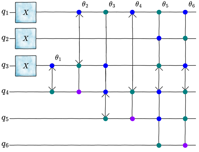
Figure 4: Sparse quantum data loader. An example with ($n=6,s=7$) for a vector $\vec{x}\in\mathbb{R}^{64}$ with only $7$ non-vanishing entries at positions $7,11,14,19,26,37,58$. Colours are used to indicate the input (blue), output (green), and control (violet) qubits of each gRBS gate in Eq. (4) and angles are computed using Eq. (III.2.1) for the non-vanishing entries. The execution of Alg. 5 to construct this circuit is shown in Tab. 3. This circuit can be compiled using at most $174$ CNOTs (see Tab. 1 in App. A).

V Binary encoder

Here we show how to compose the dense HW-$k$ encoders introduced in Sec. III to achieve a binary-basis amplitude encoder. Let us assume again, for simplicity, that the goal is to encode real amplitudes $\vec{x}\in\mathbb{R}^{2^{n}}$. The generalization to complex amplitudes in the same way as in Sec. III.2.2 is straightforward.

The procedure goes as follows: (i) first initialize the circuit in the state $\ket{0^{n}}$; (ii) apply a $R_{y}$ gate in the last qubit to generate the superposition $\cos\theta_{1}\ket{0^{n}}+\sin\theta_{1}\ket{10^{n-1}}$ with the first state of HW-$1$; (iii) take $\ket{10^{n-1}}$ as the initially marked bitstring needed to construct $\operatorname{Load}_{B_{1}}(\vec{x})$ using Alg. 3; (iv) after generating all superpositions in $\operatorname{Load}_{B_{1}}(\vec{x})$, apply a controlled-$R_{y}$ gate in the last state to increase the Hamming weight by one, thereby creating the initial marked bitstring for $\operatorname{Load}_{B_{2}}(\vec{x})$; (v) repeat step (iv) until all HW-$k$ are populated and the last multi-controlled-$R_{y}$ generates the superposition with $\ket{1^{n}}$. Notice that the (multi-)controlled-$R_{y}$ gates applied between loaders $\operatorname{Load}_{B_{k}}(\vec{x})$ and $\operatorname{Load}_{B_{k+1}}(\vec{x})$ should be chosen such that the newly created bitstring is a viable initial state for the Ehrlich algorithm (see Thm. $2.4$ in [35]). Alternatively, the Hamming-weight-increasing step (iv) above could also be performed using the HW-mixing gRBS gates $R^{\mathcolor{blue}{in_{1},\ldots,in_{m}}}_{\mathcolor{teal}{out_{1},\ldots,out_{m^{\prime}}}}$ introduced in Eq. (4). However, since the necessary bitflips are local, we chose to use the cheaper multi-controlled-$R_{y}$ gates (see Tab. 1 in App. A).

An example of the binary encoder for $n=6$ qubits is shown in Fig. 5. The total CNOT count is given in the following Lemma.

Lemma V.1 (CNOT count of the binary encoder).

Our binary encoder for $\vec{x}\in\mathbb{R}^{2^{n}}$ uses

$$\#\text{ CNOTs} \leq\frac{1}{12}(13n^{4}-58n^{3}+119n^{2}-50n+120)$$

$$\quad+\sum_{k=5}^{n}\left[\binom{n}{k}(16k-22)-2\right].$$ (14)

Proof.

First, it is important to notice that the two tricks mentioned in Sec. III to reduce the number of controls (namely, to eliminate initial controls and to construct HW-($n-k$) encoders from the corresponding HW-$k$ encoder) cannot be used here, since the initial state for each $\operatorname{Load}_{B_{k}}$ in Fig. 5 contains a superposition of states. Therefore, the cost of each $\operatorname{Load}_{B_{k}}$ is given by the upper bound $\left[\binom{n}{k}-1\right]C_{k-1}$ in the general expression in Eq. (7), where $C_{k-1}$ is the cost of compiling a single ($k-1$)-controlled-$R^{\mathcolor{blue}{in}}_{\mathcolor{teal}{out}}(\theta)$ gate. After each $\operatorname{Load}_{B_{k}}$ is applied, one needs a $k$-controlled $R_{y}$ gate to increase the HW to $k+1$. The total CNOT count of the circuit is therefore $\sum_{k=0}^{n}\left\{\left[\binom{n}{k}-1\right]C_{k-1}+\xi_{k}\right\}$, where $\xi_{k}$ is the CNOT cost of a $k$-controlled $R_{y}$. Plugging the values of $C_{k-1}$ and $\xi_{k}$ in computed in App. A (see Tab. 1 for a summary and Lemmas A.1 and A.2 for the derivation) immediately leads to Eq. (V.1). The first line contains exact CNOT counts coming from $k=1$ to $4$, while the second line contains upper bounds coming from $k\geq 5$. ∎

Numerically we observe the CNOT count of Eq. (V.1) to be $\leq 8\,n\,2^{n}$ (see Fig. 7 in App. A). Asymptotically, this is the same scaling obtained by the sparse encoder from Ref. [36]. Furthermore, the CNOT-gate count $\mathcal{O}(2^{n})$ of Ref. [22] refers to amplitude encoding in the Schmidt basis with at most $2^{n/2}$ coefficients, while we explore all $2^{n}$ computational basis states.

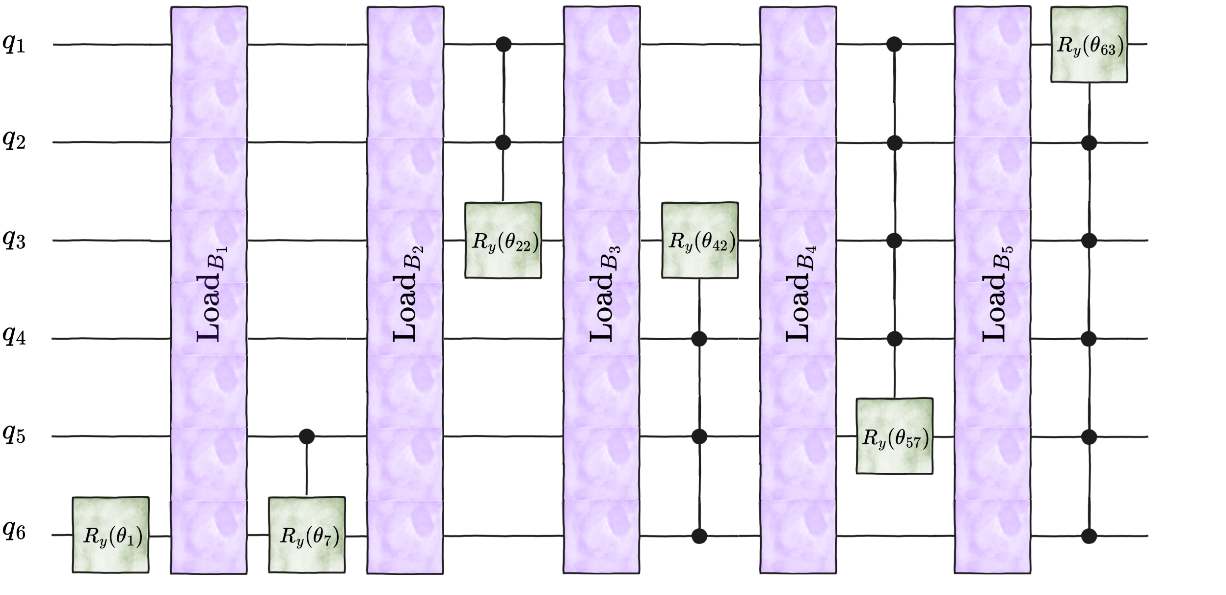
Figure 5: Binary basis amplitude encoder from HW-$k$ encoders. $d=64$-dimensional real data vector $\vec{x}$ encoded using $n=6$ qubits by stacking HW-$k$ encoders $\operatorname{Load}_{B_{k}}$ with $k=0,\ldots,6$. The circuit is initialized in the state $\ket{0^{n}}$. After each $\operatorname{Load}_{B_{k}}$, a multi-controlled-$R_{y}$ gate is applied to increase the Hamming-weight by $1$ while correctly generating a new amplitude. The newly generated state is then passed as initial state for the Ehrlich algorithm computing the circuit architecture of $\operatorname{Load}_{B_{k+1}}$ and the process is repeated until the state with all ones $\ket{111111}$ appears. The gate parameters $\theta_{1}\,\ldots,\theta_{63}$ are computed using Eq. (III.2.1) and used sequentially from left to right. See Tab. 4 in App. B for details. This circuit can be compiled using at most $1120$ CNOTs (see Tab. 1 in App. A).

VI Quantum hardware demonstration

To demonstrate our encoding protocol, we encode a $q$-Gaussian probability distribution on the Aria-1 quantum processor from IonQ [30]. The $q$-Gaussian probability density function $p_{q,\beta}(x)$, where $q\in(-\infty,\,3)$ and $\beta\in(0,\,\infty)$, is proportional to the $q$-exponential function $e_{q}\left(-\beta\,x^{2}\right)$, defined as $e^{x}\,$ if $q=1$; $\,[1+(1-q)x]^{1/(1-q)}\,$ if $q\neq 1$ and $1+(1-q)x>0$; and $0^{1/(1-q)}\,$ otherwise [37, 38, 39]. This family of distributions have a wide range of applications, e.g. nonextensive statistical mechanics [40], finance [41, 42], metrology [43], and biology [44]. It is worth to note that in general the $q$-Gaussian is a non-log-concave distribution, falling outside of the scope of other encoding strategies [12]. Here, we chose the parameters $q=3/2$ and $\beta=2$.

We use the circuit in Fig. 3 for $6$ qubits and Hamming weight $k=2$, which allows us to encode a data vector of size $d=\binom{6}{2}=15$. This vector corresponds to a discretization of the distribution truncated to the interval $x\in[-2,2]$. For this circuit, the first $4$ parameterized rotations are uncontrolled RBS gates, while the last $10$ RBSs require $1$ control each. Each RBS gate is compiled using $2$ CNOT gates, while each controlled-RBS requires $6$ CNOTs (see Tab. 1 in App. A). Thus, we expect the initial $4$ data points encoded to be more resilient to the noisy implementation on NISQ devices. Furthermore, due to the structure of the hyperspherical coordinate system in Eq. (III.2.1), which associates a larger number of sine and cosine factor to the last vector elements than to the initial ones, we expect the last elements to suffer more from hardware noise due to all the previously applied (controlled)-RBS gates.

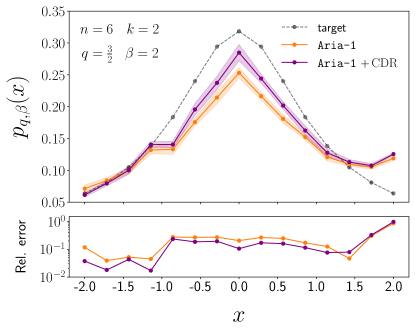
Figure 6: Experimental deployment on IonQ . (Top) Experimental implementation of the encoding of a $q$-Gaussian probability distribution $p_{q,\beta}(x)$ on IonQ ’s Aria-1 processor. This type of distributions are not log-concave, falling out of the scope of standard techniques. In Fig. 3 we show the circuit deployed, with $n=6$ and $k=2$. Domain of $p_{q,\beta}(x)$ was truncated on $x\in[-2,2]$ and discretized into $15$ points (dashed black line). Solid purple (orange) line represent experimental result with (without) using Clifford Data Regression ($\mathrm{CDR}$) as an error mitigation technique. Shaded areas represent uncertainty regions estimated via bootstrapping. (Bottom) Relative error of experimental implementation of $p_{q,\beta}(x)$ w.r.t. the target function, in log scale.

In Fig. 6, we show the results of the experimental implementation. In the top panel we plot the probability distribution estimated from the experiment by running the circuit $10^{4}$ times and measuring in the computational basis on each qubit to recover the encoded data. The solid orange line shows the empirical probability distribution estimated from the raw experimental data from the Aria-1 quantum processor. The solid purple line shows the estimated probability distribution after Clifford Data Regression [31, 32] was used for error mitigation (see App. C for details). The dashed black line shows the ideal target distribution. All relative errors with respect to the target distribution are plotted in Fig. 6 (Bottom) in log scale. We see that, starting from $x=-2$, the initial four points encoded are in good agreement with their target counterparts, while a jump in relative error of approximately one order of magnitude happens from the fourth to the fifth data point (when the first controlled-RBS is applied). This confirms the intuition that controlled-RBS gates heavily affect the fidelity of our encoding on NISQ devices. We also highlight the significant increase in relative error of the last encoded data points, which, as mentioned before, is attributed to the structure of hyperspherical coordinates.

VII Conclusions

We provide an efficient and explicit classical algorithm to construct, gate by gate, a quantum circuit that uploads an arbitrary data vector into a subspace of fixed Hamming-weight quantum states. The quantum circuit uses the minimum number of parameterized gates needed to express generic data of a given dimension. The construction uses generalized RBS gates and allows us to precisely state the quantum resources needed for its execution, as well as deploy a proof-of-concept instance on real quantum hardware. We also provide the tools needed to further explore quantum encoders for this subspace and beyond.

As shown for the sparse and binary encoder, our HW-$k$ encoder can be used as a subroutine to power more complex algorithms. These two examples are but a small sample, and future work will explore more avenues. Still, we remark on the importance of the binary encoding, as most algorithms that would benefit from robust state preparation work in this basis. Other encoding schemes, such as the unary-basis encoder, can deploy basis change circuits [45] to allow for further post-processing. A generalization of this circuit to the HW-$k$ basis would open new possibilities for more efficient general state preparation.

Furthermore, our algorithm brings interesting implications from the lens of quantum machine learning. Variational ansatze that explore a constrained space are popular due to their ability to mitigate barren plateaus. Algorithms with space compression that goes beyond linear, as is the case with our HW-$k$ encoder, are also a promising direction for other machine learning schemes [46], and shows how exploring these subspaces can be successful.

Lastly, we believe that explicit constructive algorithms for state preparation, with precise analysis on the quantum resources required, are essential to reach useful quantum advantage.

Note added.

We note that during the completion of this paper an independent work [47] appeared within the context of Bethe state preparation for integrable spin chains. Their results have partial overlap with our HW-$k$ encoders for dense data presented in Sec. III.

VIII Acknowledgments

We thank Jadwiga Wilkens for the availability of the Quantum Circuit Library [48].

Appendix A Gate compilations and CNOT counts

	$R_{y}(\theta)$	$R^{\mathcolor{blue}{in}}_{\mathcolor{teal}{out}}(\theta)$	$R^{\mathcolor{blue}{in}}_{\mathcolor{teal}{out}}(\theta,\phi)$	$R^{\mathcolor{blue}{in_{1},\ldots,in_{m}}}_{\mathcolor{teal}{out_{1},\ldots,out_{m^{\prime}}}}(\theta)$	$R^{\mathcolor{blue}{in_{1},\ldots,in_{m}}}_{\mathcolor{teal}{out_{1},\ldots,out_{m^{\prime}}}}(\theta,\phi)$
$\ell=0$	$0$	$2$	$2$	$\leq 18(m+m^{\prime})-42$	$\leq 22(m+m^{\prime})-20$
$\ell=1$	$2$	$6$	$6$	$\leq 18(m+m^{\prime})-26$	$\leq 22(m+m^{\prime})$
$\ell=2$	$4$	$10$	$14$	$\leq 18(m+m^{\prime})-10$	$\leq 22(m+m^{\prime})+20$
$\ell=3$	$12$	$26$	$38$	$\leq 18(m+m^{\prime})+6$	$\leq 22(m+m^{\prime})+40$
$\ell=4$	$36$	$\leq 58$	$\leq 84$	$\leq 18(m+m^{\prime})+22$	$\leq 22(m+m^{\prime})+60$
$\ell\geq 5$	$\leq 16\ell-24$	$\leq 16\ell-6$	$\leq 20\ell+4$	$\leq 18(m+m^{\prime})+16\ell-42$	$\leq 22(m+m^{\prime})+20\ell-20$

Table 1: CNOT count of multi-controlled $R_{y}$, RBS and gRBS gates used throughout this work. Details are provided in Sec. A. For each multi-controlled-RBS and gRBS gate the CNOT count corresponds to the best between the two compilations in Figs. 1 and 2. For multi-controlled-$R_{y}$ gates we use the CNOT counts provided in [19, 49]. The numbers in the second column are the $\xi_{\ell}$ in Lemma A.1, while the second and third columns correspond to $C_{\ell}$ used in Eq. (7) for the real and complex cases, respectively.

Here we compute the CNOT cost of the generalized RBS gate (4) and its multi-controlled versions. The following auxiliary Lemma about the CNOT cost of multi-controlled single-qubit gates will be useful.

Lemma A.1 (CNOT cost of a generic multi-controlled single-qubit gate).

Let $\xi_{\ell}(U)$ denote the number of CNOT gates to implement a $\ell$-controlled generic single-qubit gate $U$, where $\ell=0$ corresponds to no control. Then $\xi_{0}(U)=0,\xi_{1}(U)=2,\xi_{2}(U)=4,\xi_{3}(U)=12,\xi_{4}(U)=36$, and $\xi_{\ell}(U)\leq 20\ell-18$ for $\ell\geq 5$. Moreover, if $U=R_{y}(\theta)$ or $U=R_{z}(\theta)$ the bound for $\ell\geq 5$ can be improved to $\xi_{\ell}(R_{y})\leq 16\ell-24$.

Proof.

Exact compilations for $1\leq\ell\leq 4$ follow from Ref. [19, 50]. The upper bounds for $\ell\geq 5$ are given in [49]. ∎

The gRBS gate (4) admits the two different decompositions into controlled-$R_{y}$ and $R_{z}$ gates given in Fig. 2. Using Lemma A.1, one can now compute the CNOT cost of a generic multi-controlled gRBS gate as follows.

Lemma A.2 (CNOT cost of a multi-controlledcomplex gRBS gate).

Let $\xi_{\ell}$ as in Lemma A.1 and $c_{\mathcolor{violet}{ctrl_{1},\ldots,ctrl_{\ell}}}R^{\mathcolor{blue}{in_{1},\ldots,in_{m}}}_{\mathcolor{teal}{out_{1},\ldots,out_{m^{\prime}}}}(\theta,\phi)$ be a $\ell$-controlled complex gRBS gate, where $\ell=0$ corresponds to no control. The number of CNOTs to compile this ($\ell+m+m^{\prime}$)-qubit gate for $\phi=0$ is

$$2(m+m^{\prime}-1)+\min\!\big{\{}2\,\xi_{\ell+m+m^{\prime}-2}(R_{y}),\xi_{\ell+m+m^{\prime}-1}(R_{y})\big{\}},$$

while for $\phi\neq 0$ it is

$$2(m+m^{\prime}-1)+\min\!\big{\{}4\,\xi_{\ell+m+m^{\prime}-2}(R_{y}),\xi_{\ell+m+m^{\prime}-1}(U)\big{\}}.$$

Proof.

$i)$ Case $\phi=0$: here the $R_{z}(\phi)$ gates are absent and we notice that the $\ell$ controls can act directly on the $R_{y}$ gates in Fig. 2. As a result, $c_{\mathcolor{violet}{ctrl_{1},\ldots,ctrl_{\ell}}}R^{\mathcolor{blue}{in_{1},\ldots,in_{m}}}_{\mathcolor{teal}{out_{1},\ldots,out_{m^{\prime}}}}$ is equivalent to $2(m-1)+2(m^{\prime}-1)+2$ CNOTs and two ($\ell+m+m^{\prime}-2$)-controlled $R_{y}$ gates for the compilation in Fig. 1 (Top), or $2(m-1)+2(m^{\prime}-1)+2$ CNOTs and a single ($\ell+m+m^{\prime}-1$)-controlled $R_{y}$ gate for the compilation in Fig. 1 (Bottom). The claim then follows from compiling each of these gates using Lemma A.1 and choosing the best between the two cases. Top is the best compilation for $\ell+m+m^{\prime}\leq 4$, while Bottom is the best otherwise.

$ii)$ Case $\phi\neq 0$: we first notice that the product $R_{y}(\theta)\,R_{z}(\phi)$ appearing in the compilation of Fig. 1 (Bottom) corresponds to the single-qubit rotation gate $U=e^{i\lambda W}$, where $\lambda(\theta,\phi)=\arccos(\cos\theta\cos\phi)$ and $W(\theta,\phi)=\frac{1}{\sin\lambda(\theta,\phi)}(-\sin\theta\sin\phi\,X+\sin\theta\cos\phi\,Y+\cos\theta\sin\phi\,Z)$. The proof then proceeds identically to Case $i)$. Top is the best compilation for $\ell+m+m^{\prime}=2$, while Bottom is the best otherwise. ∎

Explicit CNOT counts for all the gates used throughout this work are summarized in Table 1. In addition, Fig. 7 shows the asymptotic behavior $\sim 8\,n\,2^{n}$ of the total gate count for the binary encoder (see Lemma V.1 in the main text).

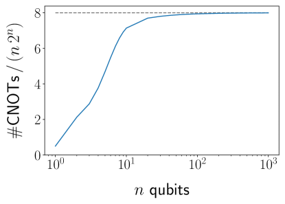
Figure 7: CNOT-gate count of the binary encoder. CNOT-gate count from Eq. (V.1) in Lemma V.1 as a function of number of qubits (in log scale). We used the $cR_{y}$ compilation for RBS in Tab. 1. We observe an asymptotic behavior towards $8\,n\,2^{n}$ for large $n$.

Appendix B Explicit examples of bitstring generation

Here we present three tables illustrating with explicit examples the execution of the classical algorithms used to generate the quantum circuits for our HW encoder algorithms. Each table corresponds to one of the figures present in the main text, namely: Table 2 illustrates the real dense encoder (Alg. 3) and corresponds to Fig. 3; Table 3 illustrates the real sparse encoder (Alg. 5) and corresponds to Fig. 4; finally, Table 4 illustrates the binary encoder that combines the dense HW-$k$ for all possible $k\in[0,n]$ and corresponds to Fig. 5.

[columns-width=1.1cm,hlines] ¿*1ccccccc $q_{6}$ & $q_{5}$ $q_{4}$ $q_{3}$ $q_{2}$ $q_{1}$ Gate

$\mathcolor{violet}{\overline{1}}$ $\mathcolor{blue}{\overline{1}}$ $0$ $0$ $0$ $\mathcolor{teal}{0}$ $\bcancel{c_{\mathcolor{violet}{6}}}\text{R}^{\mathcolor{blue}{5}}_{\mathcolor{teal}{1}}(\theta_{1})$

$\mathcolor{violet}{\overline{1}}$ $0$ $\overline{0}$ $\overline{0}$ $\mathcolor{teal}{\overline{0}}$ $\mathcolor{blue}{1}$ $\bcancel{c_{\mathcolor{violet}{6}}}\text{R}^{\mathcolor{blue}{1}}_{\mathcolor{teal}{2}}(\theta_{2})$

$\mathcolor{violet}{\overline{1}}$ $0$ $\overline{0}$ $\mathcolor{teal}{\overline{0}}$ $\mathcolor{blue}{1}$ $0$ $\bcancel{c_{\mathcolor{violet}{6}}}\text{R}^{\mathcolor{blue}{2}}_{\mathcolor{teal}{3}}(\theta_{3})$

$\mathcolor{violet}{\overline{1}}$ $0$ $\mathcolor{teal}{\overline{0}}$ $\mathcolor{blue}{1}$ $0$ $0$ $\bcancel{c_{\mathcolor{violet}{6}}}\text{R}^{\mathcolor{blue}{3}}_{\mathcolor{teal}{4}}(\theta_{4})$

$\mathcolor{blue}{\overline{1}}$ $\mathcolor{teal}{0}$ $\mathcolor{violet}{1}$ $0$ $0$ $0$ $c_{\mathcolor{violet}{4}}\text{R}^{\mathcolor{blue}{6}}_{\mathcolor{teal}{5}}(\theta_{5})$

$0$ $\mathcolor{violet}{\overline{1}}$ $\mathcolor{blue}{\overline{1}}$ $0$ $0$ $\mathcolor{teal}{0}$ $c_{\mathcolor{violet}{5}}\text{R}^{\mathcolor{blue}{4}}_{\mathcolor{teal}{1}}(\theta_{6})$

$0$ $\mathcolor{violet}{\overline{1}}$ $0$ $\overline{0}$ $\mathcolor{teal}{\overline{0}}$ $\mathcolor{blue}{1}$ $c_{\mathcolor{violet}{5}}\text{R}^{\mathcolor{blue}{1}}_{\mathcolor{teal}{2}}(\theta_{7})$

$0$ $\mathcolor{violet}{\overline{1}}$ $0$ $\mathcolor{teal}{\overline{0}}$ $\mathcolor{blue}{1}$ $0$ $c_{\mathcolor{violet}{5}}\text{R}^{\mathcolor{blue}{2}}_{\mathcolor{teal}{3}}(\theta_{8})$

$0$ $\mathcolor{blue}{\overline{1}}$ $\mathcolor{teal}{0}$ $\mathcolor{violet}{1}$ $0$ $0$ $c_{\mathcolor{violet}{3}}\text{R}^{\mathcolor{blue}{5}}_{\mathcolor{teal}{4}}(\theta_{9})$

$0$ $0$ $\mathcolor{violet}{\overline{1}}$ $\mathcolor{blue}{\overline{1}}$ $0$ $\mathcolor{teal}{0}$ $c_{\mathcolor{violet}{4}}\text{R}^{\mathcolor{blue}{3}}_{\mathcolor{teal}{1}}(\theta_{10})$

$0$ $0$ $\mathcolor{violet}{\overline{1}}$ $0$ $\mathcolor{teal}{\overline{0}}$ $\mathcolor{blue}{1}$ $c_{\mathcolor{violet}{4}}\text{R}^{\mathcolor{blue}{1}}_{\mathcolor{teal}{2}}(\theta_{11})$

$0$ $0$ $\mathcolor{blue}{\overline{1}}$ $\mathcolor{teal}{0}$ $\mathcolor{violet}{1}$ $0$ $c_{\mathcolor{violet}{2}}\text{R}^{\mathcolor{blue}{4}}_{\mathcolor{teal}{3}}(\theta_{12})$

$0$ $0$ $0$ $\mathcolor{violet}{\overline{1}}$ $\mathcolor{blue}{\overline{1}}$ $\mathcolor{teal}{0}$ $c_{\mathcolor{violet}{3}}\text{R}^{\mathcolor{blue}{2}}_{\mathcolor{teal}{1}}(\theta_{13})$

$0$ $0$ $0$ $\color[rgb]{0,0,1}{\overline{1}}$ $\mathcolor{teal}{0}$ $\mathcolor{violet}{1}$ $c_{\mathcolor{violet}{1}}\text{R}^{\mathcolor{blue}{3}}_{\mathcolor{teal}{2}}(\theta_{14})$

$0$ $0$ $0$ $0$ $1$ $1$

Table 2: Illustration of the dense HW-$k$ encoder (Alg. 3) for $\bm{n=6}$ qubits and $\bm{k=2}$. Here $\vec{x}\in\mathbb{R}^{d}$ with $d=\binom{n}{k}=15$. The order of bitstrings is given by Alg. 1. Marked bits are represented with a bar. Qubit indices are enumerated from left to right, $c_{\mathcolor{violet}{ctrl}}\text{R}^{\mathcolor{blue}{in}}_{\mathcolor{teal}{out}}$ denotes an RBS on input qubit $\mathcolor{blue}{in}$, output qubit $\mathcolor{teal}{out}$ controlled by qubit(s) $\mathcolor{violet}{ctrl}$, and $\theta_{i}$ given by Eq. (III.2.1). Unnecessary $\mathcolor{violet}{ctrl}$ qubits removed by Alg. 2 are denoted as $\bcancel{c_{\mathcolor{violet}{ctrl}}}$.

[columns-width=1.1cm,hlines]¿*7c $q_{6}$ & $q_{5}$ $q_{4}$ $q_{3}$ $q_{2}$ $q_{1}$ Gate

$0$ $0$ $\color[rgb]{0,.5,.5}{0}$ $\color[rgb]{0,0,1}{1}$ $\color[rgb]{.5,0,.5}{1}$ $\color[rgb]{.5,0,.5}{1}$ $c_{\bcancel{\mathcolor{violet}{1}},\bcancel{\mathcolor{violet}{2}}}\text{R}^{\mathcolor{blue}{3}}_{\mathcolor{teal}{4}}(\theta_{1})$

$0$ $0$ $\color[rgb]{.5,0,.5}{1}$ $\color[rgb]{0,.5,.5}{0}$ $\color[rgb]{.5,0,.5}{1}$ $\color[rgb]{0,0,1}{1}$ $c_{\bcancel{\mathcolor{violet}{2}},\mathcolor{violet}{4}}\text{R}^{\mathcolor{blue}{1}}_{\mathcolor{teal}{3}}(\theta_{2})$

${0}$ $\color[rgb]{0,.5,.5}{0}$ $\color[rgb]{0,0,1}{1}$ $\color[rgb]{0,0,1}{1}$ $\color[rgb]{.5,0,.5}{1}$ $\color[rgb]{0,.5,.5}{0}$ $c_{\bcancel{\mathcolor{violet}{2}}}\text{R}^{\mathcolor{blue}{3},\mathcolor{blue}{4}}_{\mathcolor{teal}{1},\mathcolor{teal}{5}}(\theta_{3})$

$0$ $\color[rgb]{.5,0,.5}{1}$ $\color[rgb]{0,.5,.5}{0}$ $0$ $\color[rgb]{.5,0,.5}{1}$ $\color[rgb]{0,0,1}{1}$ $c_{\bcancel{\mathcolor{violet}{2}},\mathcolor{violet}{5}}\text{R}^{\mathcolor{blue}{1}}_{\mathcolor{teal}{4}}(\theta_{4})$

$\color[rgb]{0,.5,.5}{0}$ $\color[rgb]{0,0,1}{1}$ $\color[rgb]{0,0,1}{1}$ $\color[rgb]{0,.5,.5}{0}$ $\color[rgb]{0,0,1}{1}$ $\color[rgb]{0,.5,.5}{0}$ $\text{R}^{\mathcolor{blue}{2},\mathcolor{blue}{4},\mathcolor{blue}{5}}_{\mathcolor{teal}{1},\mathcolor{teal}{3},\mathcolor{teal}{6}}(\theta_{5})$

$\color[rgb]{.5,0,.5}{1}$ $\color[rgb]{0,.5,.5}{0}$ $\color[rgb]{0,.5,.5}{0}$ $\color[rgb]{0,0,1}{1}$ $\mathcolor{teal}{0}$ $\color[rgb]{0,0,1}{1}$ $c_{\mathcolor{violet}{6}}\text{R}^{\mathcolor{blue}{1},\mathcolor{blue}{3}}_{\mathcolor{teal}{2},\mathcolor{teal}{4},\mathcolor{teal}{5}}(\theta_{6})$

$1$ $1$ $1$ $0$ $1$ $0$

Table 3: Illustration of the sparse vector encoder (Alg. 5) for $\bm{n=6}$ qubits and $s=7$. The addresses $b_{i}$ are arranged so as to keep the HW increasing (compulsory) and minimize CNOT count with Alg. 2 (optional). The angles $\theta_{i}$ are given by Eq.(III.2.1). The first $6$ elements have $k=3$, so the controlled gRBS gates are HW-preserving, while the last has $k=4$ and requires a gRBS with $m\neq m^{\prime}$ to increase the HW by $1$.

[columns-width=0.9cm,hlines]¿*8c $q_{6}$ & $q_{5}$ $q_{4}$ $q_{3}$ $q_{2}$ $q_{1}$ Operator $k$

$0$ $0$ $0$ $0$ $0$ $0$ $R^{6}_{y}(\theta_{1})$ $0$

$\overline{1}$ $0$ $0$ $0$ $0$ $0$ $\operatorname{Load}_{B_{1}}$ $1$

$\vdots$ $\vdots$ $\vdots$ $\vdots$ $\vdots$ $\vdots$ $\mathcolor{gray}{\{\theta_{2},...,\theta_{6}\}}$ $1$

$0$ $1$ $0$ $0$ $0$ $0$ $c_{5}R^{6}_{y}(\theta_{7})$ $1$

$\overline{1}$ $\overline{1}$ $0$ $0$ $0$ $0$ $\operatorname{Load}_{B_{2}}$ $2$

$\vdots$ $\vdots$ $\vdots$ $\vdots$ $\vdots$ $\vdots$ $\mathcolor{gray}{\{\theta_{8},...,\theta_{21}\}}$ $2$

$0$ $0$ $0$ $0$ $1$ $1$ $c_{1,2}R^{3}_{y}(\theta_{22})$ $2$

$\overline{0}$ $\overline{0}$ $\overline{0}$ $1$ $1$ $1$ $\operatorname{Load}_{B_{3}}$ $3$

$\vdots$ $\vdots$ $\vdots$ $\vdots$ $\vdots$ $\vdots$ $\mathcolor{gray}{\{\theta_{23},...,\theta_{41}\}}$ $3$

$1$ $1$ $1$ $0$ $0$ $0$ $c_{4,5,6}R^{3}_{y}(\theta_{42})$ $3$

$\overline{1}$ $\overline{1}$ $\overline{1}$ $\overline{1}$ $0$ $0$ $\operatorname{Load}_{B_{4}}$ $4$

$\vdots$ $\vdots$ $\vdots$ $\vdots$ $\vdots$ $\vdots$ $\mathcolor{gray}{\{\theta_{43},...,\theta_{56}\}}$ $4$

$0$ $0$ $1$ $1$ $1$ $1$ $c_{1,2,3,4}R^{5}_{y}(\theta_{57})$ $4$

$\overline{0}$ $1$ $1$ $1$ $1$ $1$ $\operatorname{Load}_{B_{5}}$ $5$

$\vdots$ $\vdots$ $\vdots$ $\vdots$ $\vdots$ $\vdots$ $\mathcolor{gray}{\{\theta_{58},...,\theta_{62}\}}$ $5$

$1$ $1$ $1$ $1$ $1$ $0$ $c_{2,3,4,5,6}R^{1}_{y}(\theta_{63})$ $5$

$1$ $1$ $1$ $1$ $1$ $1$ $6$

Table 4: Illustration of the binary encoder for $n=6$ qubits. The initial bitstring has $k=0$ and (controlled) $R_{y}$ gates are used to increase the HW by $1$. The first bitstring with HW-($k+1$) has one bit difference from the final bitstring of the Ehrlich algorithm with HW-$k$. Operators $\operatorname{Load}_{B_{k}}$ fill up the subspace of HW-$k$, and the algorithm stops after reaching $k=n$. Angles $\theta_{i}$ are given by Eq.(III.2.1), $\theta_{i}$ are used in $R_{y}$ gates and $\mathcolor{gray}{\theta_{i}}$ are used in $\operatorname{Load}_{B_{k}}$. Total number of parameters is $2^{n}-1$.

Appendix C Clifford Data Regression

Clifford Data Regression (CDR) is a data-driven protocol to mitigate errors on expectation values estimated on NISQ devices [31, 32]. The protocol to implement CDR takes as inputs a quantum circuit $\mathcal{C}$ and an expectation value $\mu^{(0)}$ and repeats the following primitive: (i) construct a near-Clifford circuit by randomly replacing most, if not all, non-Clifford gates in the original circuit by Clifford gates; (ii) run both classical simulation and noisy implementation of the near-Clifford circuit, obtaining a set $\mathcal{S}$ containing new expectation values $\mu_{\textup{noiseless}}$ and $\mu_{\textup{noisy}}$ coming from the noiseless and noisy circuit, respectively,

$$\mathcal{S}\coloneqq\left\{\left(\mu_{\textup{noisy}}^{(j)},\,\mu_{\textup{noiseless}}^{(j)}\right)\right\}_{j\in\left[\,\absolutevalue{\mathcal{S}}\,\right]}\,,$$ (15)

where $\absolutevalue{\mathcal{S}}$ is the cardinality of the set $\mathcal{S}$. The next step is to fit a regression model $f$ on $\mathcal{S}$ such that

$$\mu_{\textup{noiseless}}^{(j)}\approx f_{\mathcal{S}}\left(\mu_{\textup{noisy}}^{(j)}\right),\,\forall\,j\in\left[\,\absolutevalue{\mathcal{S}}\,\right]\,.$$ (16)

With that at hand, after executing the original circuit on the noisy hardware and obtaining the noisy expectation value $\mu_{noisy}^{(0)}$, the last step is to use the fitted model to get an error-mitigated version of $\mu_{\textup{noisy}}^{(0)}$, i.e.

$$\mu_{\textup{mitigated}}^{(0)}\approx f_{\mathcal{S}}\left(\mu_{\textup{noisy}}^{(0)}\right)\,.$$ (17)

The error-mitigated expectation value $\mu_{\textup{mitigated}}^{(0)}$ is then the final empirical estimator of $\mu^{(0)}$.

In our proof-of-principle demonstration described in Sec. VI, we implemented CDR following the protocol detailed above training a linear model for each expectation value separately. In doing so, we first compiled the original circuit in a way that the only non-Clifford gates present were $R_{y}$ rotations. We call replacement rate, $r\in(0,1)$, the number of $R_{y}$ gates replaced in the original circuit in order to generate each near-Clifford circuit $j$. We created our set of near-Clifford circuits using replacement rates $r\in\{0.79,\,0.83,\,0.90,\,0.95,\,1.00\}$ and sampling $50$ circuits per replacement rate, totaling $\absolutevalue{\mathcal{S}}=250$ data points. The random Cliffords to be inserted were sampled uniformly from the set of all possible single-qubit Clifford gates. We also uniformly sampled the positions in the circuit of the $R_{y}$ gates that were replaced. The set (15) was generated by classically simulating noiseless circuits locally while simulating the same circuits using the IonQ ’s proprietary noise models on IonQ ’s Quantum Cloud [51]. Every probability estimated from the hardware experiment was treated as an expectation value over a rank-$1$ projector in the computational basis and the mitigation procedure followed as described above by fitting one regression model per probability.

References

- Anselmetti et al. [2021] G.-L. R. Anselmetti, D. Wierichs, C. Gogolin, and R. M. Parrish, Local, expressive, quantum-number-preserving VQE ansätze for fermionic systems, New Journal of Physics 23, 113010 (2021).
- Arrazola et al. [2022] J. M. Arrazola, O. Di Matteo, N. Quesada, S. Jahangiri, A. Delgado, and N. Killoran, Universal quantum circuits for quantum chemistry, Quantum 6, 742 (2022).
- Monbroussou et al. [2023] L. Monbroussou, J. Landman, A. B. Grilo, R. Kukla, and E. Kashefi, Trainability and Expressivity of Hamming-Weight Preserving Quantum Circuits for Machine Learning (2023), arXiv:2309.15547 [quant-ph] .
- Cherrat et al. [2024] E. A. Cherrat, I. Kerenidis, N. Mathur, J. Landman, M. Strahm, and Y. Y. Li, Quantum Vision Transformers, Quantum 8, 1265 (2024).
- Ramos-Calderer et al. [2021] S. Ramos-Calderer, A. Pérez-Salinas, D. García-Martín, C. Bravo-Prieto, J. Cortada, J. Planagumà, and J. I. Latorre, Quantum unary approach to option pricing, Physical Review A 103, 10.1103/physreva.103.032414 (2021).
- Johri et al. [2021] S. Johri, S. Debnath, A. Mocherla, A. Singk, A. Prakash, J. Kim, and I. Kerenidis, Nearest centroid classification on a trapped ion quantum computer, npj Quantum Information 7, 122 (2021).
- Kerenidis et al. [2022] I. Kerenidis, J. Landman, and N. Mathur, Classical and Quantum Algorithms for Orthogonal Neural Networks (2022), arXiv:2106.07198 [quant-ph] .
- Kerenidis and Prakash [2022] I. Kerenidis and A. Prakash, Quantum machine learning with subspace states (2022), arXiv:2202.00054 [quant-ph] .
- Zhang et al. [2023] H. Zhang, L. Wan, S. Ramos-Calderer, Y. Zhan, W.-K. Mok, H. Cai, F. Gao, X. Luo, G.-Q. Lo, L. C. Kwek, J. I. Latorre, and A. Q. Liu, Efficient option pricing with a unary-based photonic computing chip and generative adversarial learning, Photon. Res. 11, 1703 (2023).
- Ventura and Martinez [1999] D. Ventura and T. Martinez, Initializing the amplitude distribution of a quantum state, Foundations of Physics Letters 12, 547 (1999).
- Long and Sun [2001] G.-L. Long and Y. Sun, Efficient scheme for initializing a quantum register with an arbitrary superposed state, Physical Review A 64, 014303 (2001).
- Grover and Rudolph [2002] L. Grover and T. Rudolph, Creating superpositions that correspond to efficiently integrable probability distributions, arXiv preprint quant-ph/0208112 (2002).
- Lloyd and Weedbrook [2018] S. Lloyd and C. Weedbrook, Quantum generative adversarial learning, Physical review letters 121, 040502 (2018).
- Dallaire-Demers and Killoran [2018] P.-L. Dallaire-Demers and N. Killoran, Quantum generative adversarial networks, Physical Review A 98, 012324 (2018).
- Mitarai et al. [2019] K. Mitarai, M. Kitagawa, and K. Fujii, Quantum analog-digital conversion, Physical Review A 99, 012301 (2019).
- Holmes and Matsuura [2020] A. Holmes and A. Y. Matsuura, Efficient quantum circuits for accurate state preparation of smooth, differentiable functions, in 2020 IEEE International Conference on Quantum Computing and Engineering (QCE) (IEEE, 2020) pp. 169–179.
- Araujo et al. [2021] I. F. Araujo, D. K. Park, F. Petruccione, and A. J. da Silva, A divide-and-conquer algorithm for quantum state preparation, Scientific reports 11, 6329 (2021).
- Jaques and Rattew [2023] S. Jaques and A. G. Rattew, QRAM: A Survey and Critique (2023), arXiv:2305.10310 [quant-ph] .
- Barenco et al. [1995] A. Barenco, C. H. Bennett, R. Cleve, D. P. DiVincenzo, N. Margolus, P. Shor, T. Sleator, J. A. Smolin, and H. Weinfurter, Elementary gates for quantum computation, Physical Review A 52, 3457–3467 (1995).
- Kitaev [1997] A. Y. Kitaev, Quantum computations: algorithms and error correction, Russian Mathematical Surveys 52, 1191 (1997).
- Boykin et al. [1999] P. O. Boykin, T. Mor, M. Pulver, V. Roychowdhury, and F. Vatan, On Universal and Fault-Tolerant Quantum Computing (1999), arXiv:quant-ph/9906054 [quant-ph] .
- Plesch and Brukner [2011] M. Plesch and Č. Brukner, Quantum-state preparation with universal gate decompositions, Physical Review A 83, 032302 (2011).
- Huggins et al. [2021] W. J. Huggins, S. McArdle, T. E. O’Brien, J. Lee, N. C. Rubin, S. Boixo, K. B. Whaley, R. Babbush, and J. R. McClean, Virtual Distillation for Quantum Error Mitigation, Phys. Rev. X 11, 041036 (2021).
- Gibbs et al. [2022] J. Gibbs, K. Gili, Z. Holmes, B. Commeau, A. Arrasmith, L. Cincio, P. J. Coles, and A. Sornborger, Long-time simulations with high fidelity on quantum hardware, npj Quantum Information 8, 135 (2022).
- Zhao et al. [2023] L. Zhao, J. Goings, K. Shin, W. Kyoung, J. I. Fuks, J.-K. Kevin Rhee, Y. M. Rhee, K. Wright, J. Nguyen, J. Kim, et al., Orbital-optimized pair-correlated electron simulations on trapped-ion quantum computers, npj Quantum Information 9, 60 (2023).
- Jain et al. [2024] N. Jain, J. Landman, N. Mathur, and I. Kerenidis, Quantum fourier networks for solving parametric pdes, Quantum Science and Technology 9, 035026 (2024).
- He et al. [2023] Z. He, R. Shaydulin, S. Chakrabarti, D. Herman, C. Li, Y. Sun, and M. Pistoia, Alignment between initial state and mixer improves QAOA performance for constrained optimization, npj Quantum Information 9, 10.1038/s41534-023-00787-5 (2023).
- Cherrat et al. [2023] E. A. Cherrat, S. Raj, I. Kerenidis, A. Shekhar, B. Wood, J. Dee, S. Chakrabarti, R. Chen, D. Herman, S. Hu, P. Minssen, R. Shaydulin, Y. Sun, R. Yalovetzky, and M. Pistoia, Quantum deep hedging, Quantum 7, 1191 (2023).
- Ragone et al. [2023] M. Ragone, B. N. Bakalov, F. Sauvage, A. F. Kemper, C. O. Marrero, M. Larocca, and M. Cerezo, A Unified Theory of Barren Plateaus for Deep Parametrized Quantum Circuits (2023), arXiv:2309.09342 [quant-ph] .
- IonQ Inc. [2024a] IonQ Inc., IonQ Aria (2024a).
- Czarnik et al. [2021] P. Czarnik, A. Arrasmith, P. J. Coles, and L. Cincio, Error mitigation with clifford quantum-circuit data, Quantum 5, 592 (2021).
- Lowe et al. [2021] A. Lowe, M. H. Gordon, P. Czarnik, A. Arrasmith, P. J. Coles, and L. Cincio, Unified approach to data-driven quantum error mitigation, Physical Review Research 3, 10.1103/physrevresearch.3.033098 (2021).
- Note [1] We notice that the gate is preferred by some authors and referred to as Givens rotations.
- Landman et al. [2022] J. Landman, N. Mathur, Y. Y. Li, M. Strahm, S. Kazdaghli, A. Prakash, and I. Kerenidis, Quantum methods for neural networks and application to medical image classification, Quantum 6, 881 (2022).
- Even [1973] S. Even, Algorithmic Combinatorics (The Macmillan Company, 1973).
- de Veras et al. [2022] T. M. L. de Veras, L. D. da Silva, and A. J. da Silva, Double sparse quantum state preparation, Quantum Information Processing 21, 204 (2022).
- Tsallis [1988] C. Tsallis, Possible generalization of boltzmann-gibbs statistics, Journal of statistical physics 52, 479 (1988).
- Tsallis et al. [1995] C. Tsallis, S. V. F. Levy, A. M. C. Souza, and R. Maynard, Statistical-Mechanical Foundation of the Ubiquity of Lévy Distributions in Nature, Phys. Rev. Lett. 75, 3589 (1995).
- Prato and Tsallis [1999] D. Prato and C. Tsallis, Nonextensive foundation of Lévy distributions, Phys. Rev. E 60, 2398 (1999).
- Tsallis [2009] C. Tsallis, Nonadditive entropy and nonextensive statistical mechanics - An overview after 20 years, Brazilian Journal of Physics 39, 337 (2009).
- Borland [2002] L. Borland, Option Pricing Formulas Based on a Non-Gaussian Stock Price Model, Physical Review Letters 89, 10.1103/physrevlett.89.098701 (2002).
- Borland [2004] L. Borland, The Pricing of Stock Options, in Nonextensive Entropy: Interdisciplinary Applications (Oxford University Press, 2004).
- Witkovský [2023] V. Witkovský, Characteristic Function of the Tsallis -Gaussian and Its Applications in Measurement and Metrology, Metrology 3, 222–236 (2023).
- Fernández-Navarro et al. [2011] F. Fernández-Navarro, C. Hervás-Martínez, M. Cruz-Ramírez, P. A. Gutiérrez, and A. Valero, Evolutionary -Gaussian Radial Basis Function Neural Network to determine the microbial growth/no growth interface of Staphylococcus aureus, Applied Soft Computing 11, 3012 (2011).
- Ramos-Calderer [2022] S. Ramos-Calderer, Efficient quantum interpolation of natural data, Physical Review A 106, 062427 (2022).
- Sciorilli et al. [2024] M. Sciorilli, L. Borges, T. L. Patti, D. García-Martín, G. Camilo, A. Anandkumar, and L. Aolita, Towards large-scale quantum optimization solvers with few qubits (2024), arXiv:2401.09421 [quant-ph] .
- Raveh and Nepomechie [2024] D. Raveh and R. I. Nepomechie, Deterministic Bethe state preparation (2024), arXiv:2403.03283 [quant-ph] .
- Wilkens [2023] J. Wilkens, Quantum Circuit Library (2023).
- Vale et al. [2023] R. Vale, T. M. D. Azevedo, I. C. S. Araújo, I. F. Araujo, and A. J. da Silva, Decomposition of Multi-controlled Special Unitary Single-Qubit Gates (2023), arXiv:2302.06377 [quant-ph] .
- Iten et al. [2016] R. Iten, R. Colbeck, I. Kukuljan, J. Home, and M. Christandl, Quantum circuits for isometries, Physical Review A 93, 10.1103/physreva.93.032318 (2016).
- IonQ Inc. [2024b] IonQ Inc., IonQ Quantum Cloud (2024b).