Convolutional L2LFlows: Generating Accurate Showers in Highly Granular Calorimeters Using Convolutional Normalizing Flows

Abstract

In the quest to build generative surrogate models as computationally efficient alternatives to rule-based simulations, the quality of the generated samples remains a crucial frontier. So far, normalizing flows have been among the models with the best fidelity. However, as the latent space in such models is required to have the same dimensionality as the data space, scaling up normalizing flows to high dimensional datasets is not straightforward. The prior L2LFlows approach successfully used a series of separate normalizing flows and sequence of conditioning steps to circumvent this problem. In this work, we extend L2LFlows to simulate showers with a 9-times larger profile in the lateral direction. To achieve this, we introduce convolutional layers and U-Net-type connections, move from masked autoregressive flows to coupling layers, and demonstrate the successful modelling of showers in the ILD Electromagnetic Calorimeter as well as Dataset 3 from the public CaloChallenge dataset.

HEPHY-ML-24-02

1 Introduction

Motivated by the high computational cost of simulating particle interactions with complex detectors [1, 2], a global effort is underway to develop reliable generative surrogate models based on machine learning. To this end, network architectures based on generative adversarial networks (GANs) [3, 4, 5, 6, 7, 8, 9, 10, 11, 12, 13, 14, 15, 16, 17, 18], variational autoencoders (VAEs) [19, 20, 21, 13, 22, 23, 24, 25, 26], normalizing flows [27, 28, 29, 30, 31, 32, 33, 34, 35, 36, 37], and various types of diffusion models [38, 39, 40, 41, 42, 43, 44, 45, 46, 47, 48] have been explored (see [49] for a recent taxonomy).

Besides detector simulations, generative methods are used for various tasks in high-energy physics. These include end-to-end event generation [50, 51, 52, 53, 54, 55, 56, 57, 58, 59], phase space sampling [60, 61, 62, 63, 64, 65, 66, 67, 68, 69, 70, 71], parton showers [72, 73, 74, 75, 76, 77, 78, 79, 80, 81, 82, 83, 83, 84, 85, 86, 87], hadronization [88, 89, 90, 91, 92] and anomaly detection [93, 94, 95, 96, 97, 98, 99, 100, 101, 102, 103, 104, 105, 106].

The fast simulation of particle showers in highly granular calorimeters, as under construction for the HL-LHC and envisaged for many future collider detectors, is a particularly worthwhile application of generative methods. Simulating such calorimeter showers is typically done with Geant4 [107, 108, 109] a detailed simulation from first principles that is very demanding in terms of CPU resources due to the necessary creation and tracking of a huge number of secondary particles through the entire geometry for every shower. Highly granular calorimeters sample particle showers across many layers, where every layer consists of an absorber material followed by a sensitive materials with readout cells of $O(1-10)~{}$mm sizes. The simulation of calorimeter showers need a substantial fraction of compute power at the LHC, even with less granular calorimeters that are currently in use, giving rise for large potential cost savings with generative methods.

While normalizing flows achieve very high generative fidelity, they are so-far limited in their scalability to larger and more complex datasets. The causal conditioning in [31] was a first step in making flow-based architectures more scalable. At the core of the problem lies that normalizing flows learn a diffeomorphism between data space and latent space. While this — in combination with tractable Jacobians — allows the exact evaluation of the likelihood, it also means that the latent space and data space dimensionality are identical. As the number of trainable parameters in a fully connected architecture scales roughly with the product of the input and output dimensions of a layer, this would make data space volumes of e.g. 27k voxels prohibitively expensive. The previous L2LFlows approach [31] circumvents this issue by splitting the data among one dimension and autoregressivly conditioning subsequent layers on the previous ones. This partially mitigates the problem, as at least in one dimension the scaling now becomes linear. Accordingly, [31] demonstrated the learning of showers with 3k voxels.

However, the connections per calorimeter layer remained relatively naive. In this work, we investigate two key innovations to improve the scalability and fidelity of normalizing flows: i) convolutional layers assuming a approximate translational symmetry in lateral direction; ii) skip connections inspired by the U-net architecture [110] to further improve the flow of information and network convergence; and iii) coupling layers instead of masked autoregressive flows for fast training and inference [111, 112, 113, 114, 35] without the need of probability density distillation.

We demonstrate the feasibility of the proposed approach on the well established electromagnetic showers in the ILD first introduced in [19] as well as on dataset 3 of the CaloChallenge [115].

The rest of this paper is organized as follows: Section 2 introduces the datasets used in this work. Section 3 describes the model architecture. Section 4 introduces the metrics used to evaluate the model. Section 5 presents our results. Finally, section 6 concludes.

2 Datasets

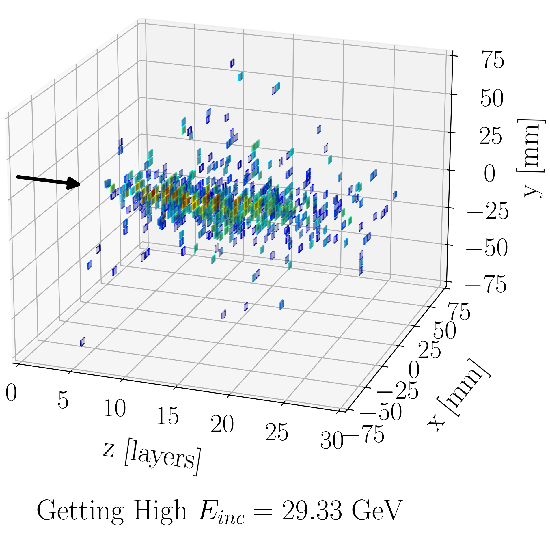
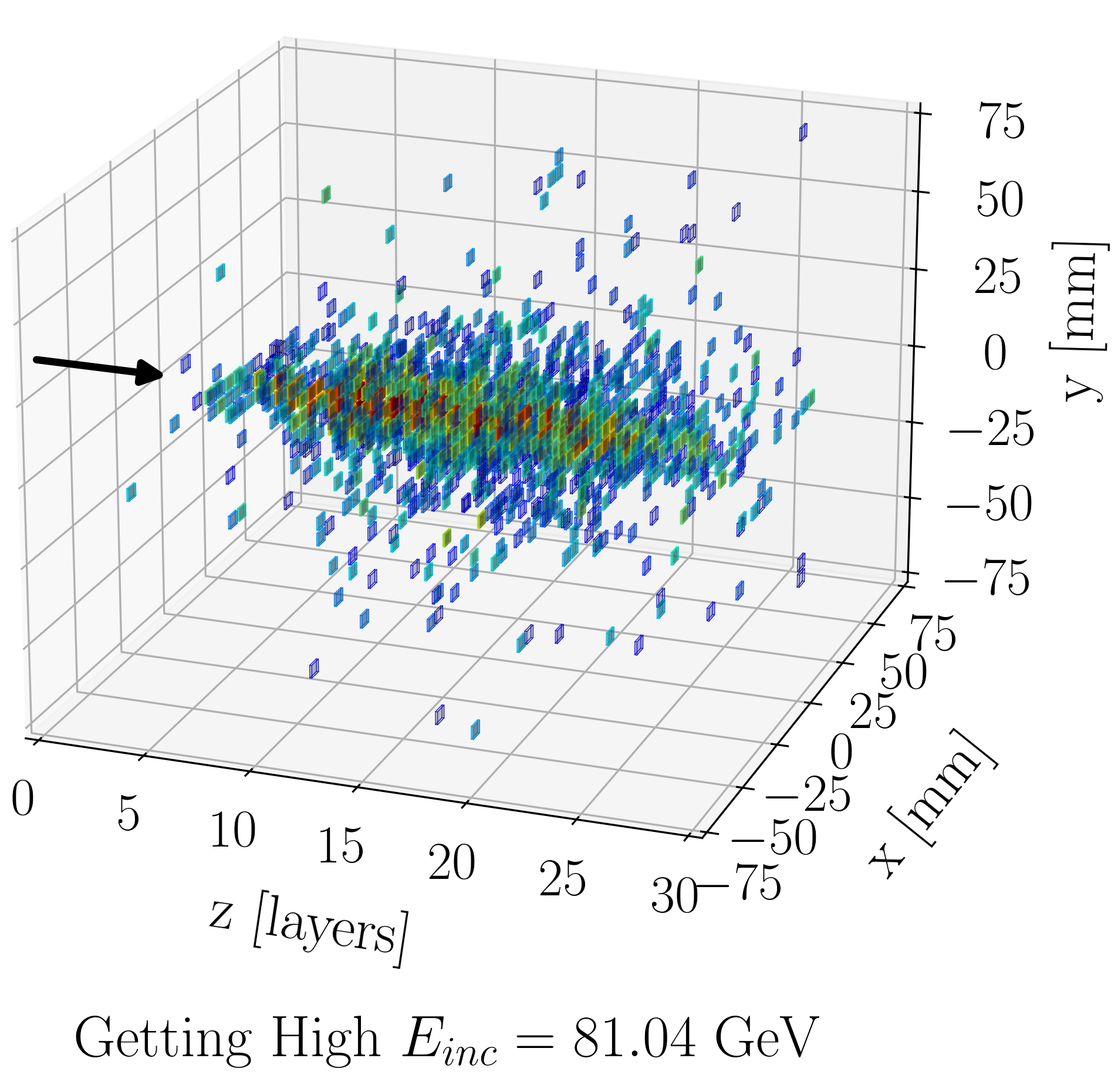
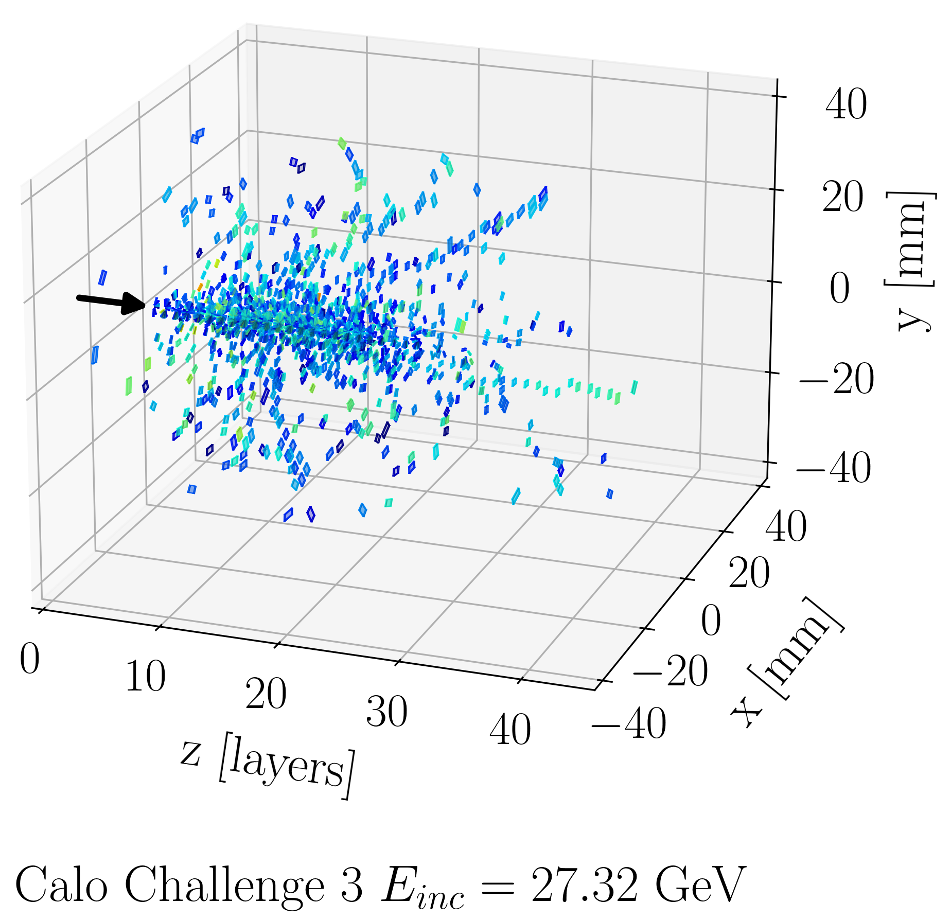
Figure 1: Visualization of single showers from the training data. The upper row shows examples from the GettingHigh dataset, the lower row from CaloChallenge dataset 3. The left examples are for low incident particle energies, the right ones for high energies.

2.1 GettingHigh

For comparison with earlier work, we use the dataset generated for [19]. It consists of photon showers in the electromagnetic calorimeter of the international large detector (ILD) [116].

Two detectors are proposed for the international linear collider (ILC), one of which is the ILD. The ILD is tailored for Particle Flow [117], an algorithm aiming to enhance detector resolution by reconstructing every individual particle. It combines precise tracking, good hermiticity, and highly granular calorimeters. The electromagnetic calorimeter (ECal) contains 30 silicon layers alternated with tungsten absorbers. It uses $5\times 5\;\text{mm}^{2}$ cells. The ILD detector’s simulation, reconstruction, and analysis rely on the iLCSoft ecosystem [118], utilizing Geant4 [107, 108, 109] and DD4hep [119] for realistic modeling.

The dataset consists of simulated photon showers with incident energies uniformly distributed from 10 to 100 GeV directed perpendicularly into the ECal. A staggered cell geometry results in small shifts between the layers, which generative models used to generate showers have to learn. A 30x30 cells bounding box around the incident point is chosen for the datasets, resulting in a data shape of 30x30x30. It has 950,000 samples, which we split into 765,000 training, 85,000 validation, and 100,000 test samples. Further details on the dataset are provided in [19].

2.2 Dataset 3 of the CaloChallenge

To facilitate the development of deep generative models for calorimeter simulation, the Fast Calorimeter Simulation Challenge (“CaloChallenge”) [115] was created. It consists of 4 calorimeter shower datasets of increasing dimensionality [120, 121, 122], all simulated with Geant4.

In this work, we work with the most complex of these datasets, dataset 3 [122]. It consists of 100,000 electron showers, with log-uniform incident energies between 1 GeV and 1 TeV that were simulated with the Par04 example geometry [123]. This is an idealized calorimeter geometry made of 90 concentric cylinders of absorber (1.4 mm of tungsten (W)) and active material (0.3 mm of silicon (Si)). Its inner radius is 800 mm and its depth is 153 mm. All showers are perpendicular to the calorimeter surface, i.e. they are in the central $\eta=0$ slice. Particle entrance position and direction determine the origin and $z$-axis of a cylindrical coordinate system and showers are discretized into voxels, with boundaries parallel to these coordinate axes.

For dataset 3 the voxels along $z$-axis corresponds to two physical layers (W-Si-W-Si) with a length of $\Delta z=3.4$ mm ($=0.8X_{0}$ of the absorber), yielding 45 read-out layers. The showers are segmented into radial ($r$) and angular ($\alpha$) bins. Dataset 3 has 18 radial segments and 50 azimuthal, for 900 voxels in each of the 45 layers (40500 total).

Each shower in the dataset consists of the total energy of the incident electron $E_{\rm inc}$ and the energy depositions recorded in each voxel $I_{ia}$, where $i$ is the layer index and $a$ is the voxel index within the layer. The minimum energy deposition in each voxel is 15.15 keV.

3 Model

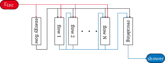
Figure 2: Diagram illustrating the overall architecture of L2LFlows. Arrows going into flows illustrate the conditional input of the flow. Arrows going out of flows illustrate what the flow has generated. The post processing is only applied to generated GettingHigh showers.

Our model is based on normalizing flows (NF) [124, 125, 126]. The idea of NFs is to learn a diffeomorphism $f$ mapping a data distribution $p(x)$ onto a simple prior distribution $q(z)$ in latent space. The density in data space then is given by the change of variable formula,

$$p(x)=q(f(x))\left|J_{x}\right|,$$ (1)

where $J_{x}$ denotes the Jacobian of $f$ evaluated at position $x$. This formula allows for likelihood-based training, where the loss function is the negative log-likelihood. To sample from an NF, one first draws samples from the prior distribution and then applies the inverse of $f$ to these samples to map them back into data space. Networks used in NF setups have to be restricted in a way that they can only learn invertible mappings and that their Jacobians are tractable.

We aim to learn the distribution of calorimeter showers conditioned on the incident energy. As in previous approaches [27, 28, 31, 33], we split this task into smaller pieces. An energy distribution flow learns the distribution of total deposited energies per calorimeter layer. For each calorimeter layer, a so-called causal flow learns the distribution of shower shapes in this particular layer. This results in $N+1$ flows for a calorimeter with $N$ layers.

To ensure consistency along the shower, later flows (in the direction of the shower evolution) are conditioned on the output of previous ones. The energy distribution flow is only conditioned on one global condition, the incident energy. The causal flows are conditioned on the incident energy, the layer energy for their layer, and the shower shape in up to five previous layers. Because the flows are conditioned on each other, during inference time, we have to draw samples from them sequentially. In this sense, it is an autoregressive model.

The original L2LFlows architecture [31] has two main drawbacks. First, it only achieves a relatively slow generation time. Second, it does not scale well to higher cardinalities. To overcome the first issue, we use coupling blocks [111, 114] similar to  [35] to speed up the generation time. Coupling-based flows can be evaluated in inverse direction almost as fast as in forward direction without requiring training a separate student model. To achieve better scalability, we used a convolution-based U-Net architecture [110] inside the coupling blocks. We will describe the architecture in more detail in the following sections.

3.1 Energy Distribution Flow

The energy distribution flow learns the distribution of layer energies, i.e., the sum of energy deposited per layer, conditioned on the incident energy. The density of this distribution can be expressed as

$$p(E_{1},\dots,E_{N}|E_{inc})$$ (2)

where $E_{1}$ to $E_{N}$ denote the layer energies and $E_{inc}$ denotes the incident energy. As this energy distribution flow is not the bottleneck of the generative task, we use the same preprocessing and architecture as in [31]. It consists of 6 MADE blocks [127, 128] with rational quadratic splines (RQS) [114]. We apply permutation layers between these MADE blocks. A logit transformation is used to preprocess the layer energies, and a log transformation is used for the incident energy.

For CaloChallenge dataset 3, we observed outliers with too high energies being generated. To mitigate this issue, we rejected and redrew all samples with a ratio between deposited and incident energy above 2.6. This threshold was exceeded 22 times during the generation of 200,000 showers.

We use PyTorch [129] and NFlows [130] to implement this model and train it using the ADAM optimizer [131]. By requiring the argument to the square root in the inversion of rational quadratic splines to be non-negative, we avoid previous numerical instabilities and can use single float instead of double float precision as was done in [27, 28, 30, 31].

3.2 Causal Flows

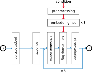
Figure 3: Diagrams illustrating the structure of a causal flow. Left: The overall structure of one single causal flow. Right: The U-Net used in the coupling blocks.

The task of the causal flows is to learn

$$p(I_{1},\dots,I_{N}|E_{1},\dots,E_{N},E_{inc})$$ (3)

where $I_{i}\in\mathbb{R}^{n\times n}$ is the shower shape in layer $i$ given by the deposited energy in each calorimeter cell. As in the original L2LFlows, this task is split up into learning

$$p(I_{i}|I_{1},\dots,I_{i-1},E_{1},\dots,E_{N},E_{inc})$$ (4)

for each layer $i$ with an individual NF. By multiplying these conditional densities, one can gain the full joint distribution. As in the original L2LFlows [31] approach, we assume approximate locality and only provide $I_{j}$ of up to five previous layers ($j\in\{i-5,i-4,i-3,i-2,i-1\})$, the energy deposited in layer $i$, and the incident energy as condition to the flows. This helps the flow to focus on the most relevant information.

The architecture of the causal flows is shown in Figure 3 on the left-hand side. Here, $x$ is $I_{i}$, the input to the shower, and $z$ is the latent space vector. Similar to CaloFlow [27], we use log and logit transformations as preprocessing. Unlike earlier flow-based models for calorimeter simulations, we do not normalize the voxel energies to one but rather rescale with a constant value. This makes it easier for the flow to learn the voxel energy spectrum. Details on preprocessing can be found in B.

In the following, we detail the additional improvements to the previous L2LFlows architecture: i) replacing MADE block with coupling layers; ii) constructing convolutional sub-network based on the U-Net architecture.

As in [35], we use a coupling-based flow [111, 114]. Similar to MADE blocks, spline coupling blocks use rational quadratic splines. Unlike MADE blocks, coupling blocks are not fully autoregressive. Instead, they split the input dimensions into two halves. The first half is fed into a sub-network that determines the spline parameters for the transformation of the second half. The first half is unchanged, allowing an inversion with a single network path, mitigating the need for a teacher-student approach [28, 33]. As for MADE blocks, the Jacobian is a triangular matrix allowing for a fast evaluation of the determinant.

In convolutional coupling flows such as in [111, 112, 113], the information is usually split along the channel dimension to preserve spatial structures. To go from calorimeter data with a single channel to several channels, we apply a so-called squeezing operation [112]. The idea is to stack pixels lying in small tiles into channels, trading in spatial dimensions for channel dimensions. To be able to concatenate input and condition, we need to bring the condition into the same shape. For this task, a small convolutional embedding network is used.

In flows like RealNVP [112] or GLOW [113], a multi-scale architecture was used to learn local features first and then regional and global features of the data. This is achieved by iteratively applying further squeezing operations. We instead use only a single squeezing operation, leaving the task of learning features on different scales to U-Nets [110]. The U-Nets are deployed within the coupling blocks to calculate the spline parameters. We found that this makes the architecture more flexible and leads to better results.

Figure 3 on the right-hand side shows an illustration of the U-Net used. The $3\times{}3$ convolutions use same padding to preserve the data size. The down-sampling operations are convolutional layers with a stride equal to the kernel size, while the up-sampling operations are inverse convolutional layers. For the CaloChallenge dataset, we use cyclic padding in the angular dimension to respect the cyclic structure of the data.

The last two parts of the architecture are activation norms and 1x1 convolutions, both of which were introduced in GLOW. Since batch and layer normalization are not directly possible in flows, activation norms provide a viable alternative. The idea is to initialize the normalization on the first batch and then update it as model parameters. 1x1 convolutions replace the permutations often used in flows to ensure the information is split up differently in each coupling block. They are initialized as orthogonal transformations. A LU decomposition ensures fast invertibility; even so, the network is not restrained to orthogonal transformations [113].

3.3 Training

As the log-likelihood is additive under joining distributions, training each flow individually is equivalent to training all flows jointly. This makes training easier and allows for straightforward parallelization on several compute nodes.

Calorimeter data are sparse, meaning that most input values are zero. This poses a problem for training flows. Since the data points live in a submanifold of the data space, the density and therefore the loss are not bounded. This problem is usually solved by adding noise. As in the original CaloFlow, we add uniform noise between zero and $1$ keV to all voxels. In addition, we fill zero voxels with log Gaussian distributed values to avoid sharp edges.

We trained one instance of the networks for 200 epochs on GettingHigh and one instance for 800 epochs on CaloChallenge dataset 3. The different amount of epochs is necessary because of the different training statistics. We applied a one-cycle learning rate scheduler [133], decoupled L2 regularization [134], and L2 gradient clipping. ADAM [131] was used as optimizer. As data augmentation, we rotated the CaloChallenge dataset 3 showers by random angles in the $x-y$ plane. This is possible because the incident particles enter the calorimeter perpendicular to its surface and no magnetic field brakes the symmetry. Further details on architecture and training are provided in A.

3.4 Postprocessing

It is not guaranteed that the causal flows produces showers that match the layer energies generated by the energy distribution flow exactly. For that reason,[27, 31] rescaled showers per-layer to match the target. However, like the authors of [33], we observe that rescaling generated CaloChallenge showers results in an excess of low energy hits due to zero voxels getting shifted above the threshold. Therefore, instead of applying postprocessing for CaloChallenge, the showers generated by the causal flows are used directly. For GettingHigh we use the same energy rescaling as in [31]. See Appendix B.3 in [31] for a detailed description.

We apply a further postprocessing step to the GettingHigh showers. This step maps the distribution of generated voxel energies onto the real voxel energy spectrum. To do so, it applies a one-dimensional function element-wise to the voxel energies. This function can be seen as a one-dimensional normalizing flow with the generated voxel energy spectrum as data distribution and the real voxel energy spectrum as latent distribution. Since we are in the one-dimensional case, this function can be evaluated numerically, and it is not necessary to learn it with a network. To speed up evaluations, we fitted a spline to the function. Further details can be found in C.

4 Metrics

4.1 Observables

Generative models aim to follow training data distributions as closely as possible. For applications in physics, it is especially interesting how accurately the distributions of certain high-level physics observables are reproduced. We give a brief description of all physics observables considered in the following. In addition to showing histograms, we also report the Wasserstein distance [79] between the ground truth and generated samples.

Hit-level Observables
Voxel energy spectrum	hit energies regardless of their position
Longitudinal profile	energy-weighted layer indexes
Radial profile	energy-weighted distances from the incident point in the $x$-$y$-plane
X profile	energy-weighted $x$ positions
Shower-level Observables
Energy ratio	total measured energy summed over all voxels divided by the incident energy
Occupancy	fraction of active voxels in a shower (Active voxels are all voxels with energies above the data-set-specific threshold.)
Center of gravity	energy-weighted mean of $x$, $y$, or longitudinal positions evaluated on each shower individually
Shower width	energy-weighted standard deviation of $x$, $y$, or longitudinal positions evaluated on each shower individually

4.2 Classifier

Histograms and one-dimensional Wasserstein distances are useful to test how well one-dimensional distributions match, but they do not account for correlations. Instead, we use classifier tests to compare generative models based on higher-dimensional distributions [27, 28, 33, 31].

We train a high-level classifier on nine observables to distinguish ML-generated and original simulation data. These are the eight shower-level observables described in the previous section and the incident energy. The incident energy allows the classifier to detect mismodelings of correlations between the incident energy, as well as the shower observables. Additionally, a classifier is trained on the hit-level information, using a convolutional architecture. Further details on the classifiers can be found in D.

As the authors of [27, 28, 33], we use the area under the receiver operating characteristic curve (AUC) and the Jensen–Shannon divergence (JSD) as performance scores.

5 Results

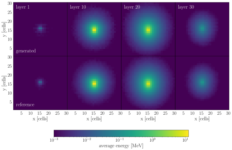
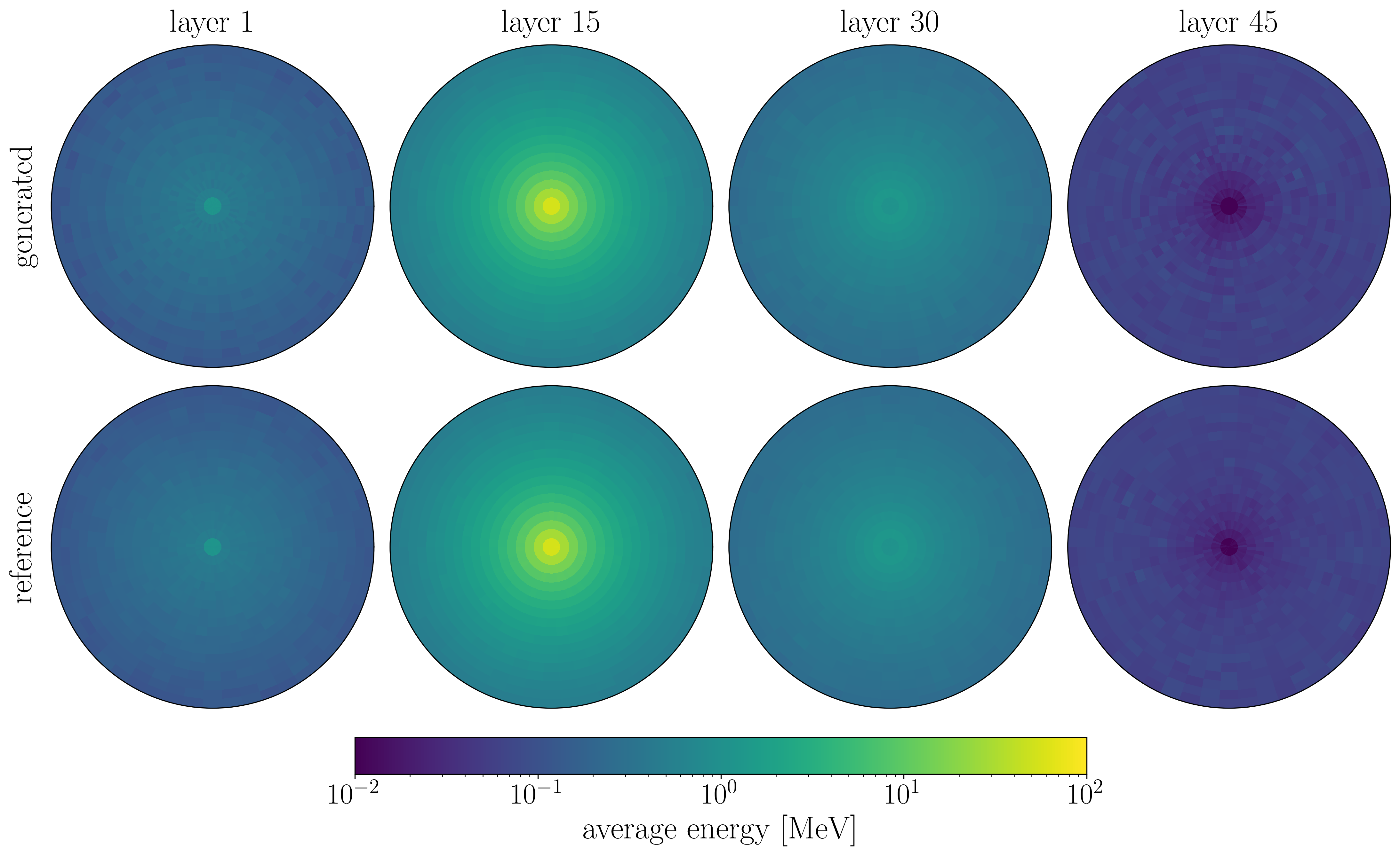
Figure 4: Average deposited energy for all cells in layer 1, 10, 20 and 30 overall flow generated (upper row) and Geant4 simulated (lower row) sample. Shown are the results for GettingHigh.

Figure 5: Average deposited energy for all cells in layer 1, 15, 30 and 45 overall flow generated (upper row) and Geant4 simulated (lower row) sample. Shown are the results for CaloChallenge datast 3.

In the following, results are reported for the GettingHigh dataset and dataset 3 of the CaloChallenge. The full $30\times 30\times 30$ voxel resolution of the GettingHigh dataset is used, which was not possible for the non-convolutional version of L2LFlows [31]. After training an instance of our model on both datasets, we draw 100,000 samples from both instances using the same incident energy distribution as the respective test data. These samples are then compared with the corresponding test data.

As a benchmark, the performance of L2LFlows is compared to the one of the BIB-AE [19]. The BIB-AE has an autoencoder-based architecture using additional adversarial critic networks and losses to improve fidelity. A kernel density estimation models the posterior distribution in latent space.

In real detectors, read-outs at small energies are dominated by noise. Therefore, an energy cut-off of half the energy of a minimal ionizing particle is applied. Energy depositions below $100$ keV are removed before comparing simulated and generated showers on GettingHigh. To be consistent with the CaloChallenge evaluation, we use $15.15$ keV as the cut-off value on CaloChallenge dataset 3.

5.1 Observables

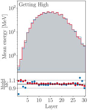
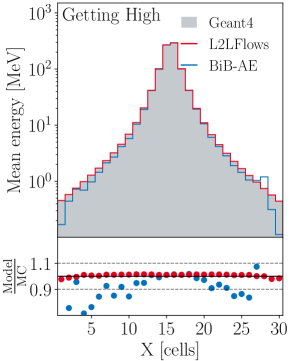
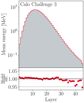
Figure 6: Top row: longitudinal (left) and $X$ profile for GettingHigh. Bottom row: longitudinal (left) and radial (right) profile for CaloChallenge dataset 3.

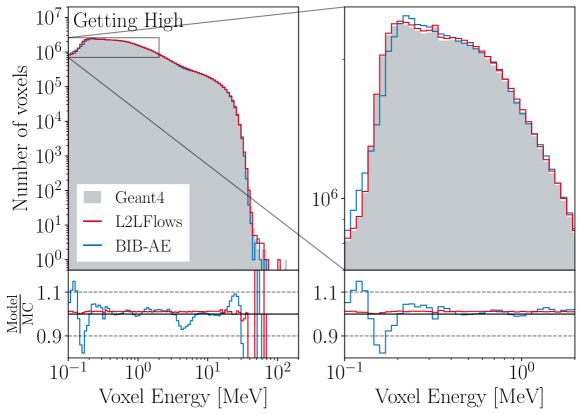
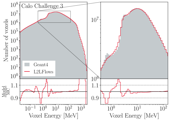
Figure 7: Cell energy spectrum.

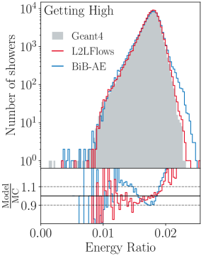
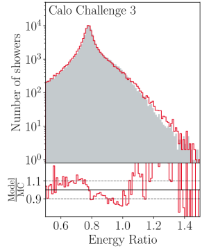
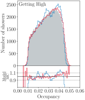
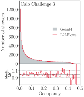
Figure 8: Top row: Total deposited energy over incident energy for GettingHigh (left) and CaloChallenge dataset 3 (right). The voxel energies in CaloChallenge dataset 3 are rescaled to account for the sampling fraction of the calorimeter. This explains the values above one and why the values for GettingHigh are way lower. Bottom row: Occupancy for GettingHigh (left) and CaloChallenge dataset 3 (right)

Figure 6 shows the longitudinal and $X$ profile for GettingHigh and the longitudinal and radial profile for CaloChallenge dataset 3. We see an excellent agreement between generated and test samples, with deviations well below five percent. The only larger deviation can be found in the first four layers of GettingHigh. The BIB-AE also agrees well with the test data. However, it can not model the $X$ profile as accurately as L2LFlows does.

Figure 7 shows the voxel energy spectrum. Here, we also see good agreements. In regions with sharp features in the reference distribution, deviations sometimes exceed $10\%$. We get a better agreement for GettingHigh than for CaloChallenge dataset 3 because post-processing is applied only for GettingHigh.

Further especially important observables are the energy ratio and the occupancy. Histograms for these observables are shown in figure 8. We see good agreements in the bulge of the distributions. In the tail regions, deviations are larger. We see an improvement compared to the BIB-AE performance. Further histograms can be found in E.

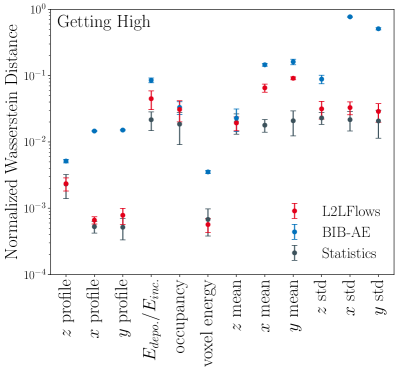
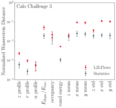
Figure 9: Wasserstein distances for several physics observables between generated and test data. The Wasserstein distances are numerically evaluated using ten batches consisting of 10,000 generated and 10,000 test set showers. Shown are the mean and the standard deviation over the ten resulting values. The gray markers show Geant4 train samples compared to Geant4 test samples. It gives us the lowest Wasserstein distance that can be resolved numerically given the amount of statistics.

The diagrams in Figure 9 show numerical evaluated one-dimensional Wasserstein distances between test data and generated data. Given are the Wasserstein distances for all observables described in section 4.1. To make the Wasserstein distance dimensionless, the distributions are standard scaled using the mean and standard deviation of the Geant4 distribution. We see a clear improvement compared to the BIB-AE in almost all observables. We also notice that for many observables, statistics are insufficient to resolve any differences between Geant4 and Flow-generated samples.

5.2 Classifier

		high level classifier		low level classifier
Dataset	Simulator	AUC	JSD	AUC	JSD
GettingHigh	L2LFlows	$.634\pm.002$	$.047\pm.002$	$.905\pm.003$	$.438\pm.009$
	BIB-AE	$.903\pm.002$	$.436\pm.005$	$\gg.999$	$.985\pm.001$
CaloChallenge 3	L2LFlows	$.686\pm.002$	$.084\pm.001$	$.983\pm.002$	$.760\pm.013$

Table 1: Results of the classifier test. Shown are the mean and standard deviation over five random network initializations.

We also conducted a classifier test to investigate multidimensional, potentially non-linear correlations. See details on this in section 4.2

The results of our classifier study are summarized in table 1. In consistency with the Wasserstein metric, we see a clear improvement of our flow model compared to the BIB-AE. The JSD value of 0.047 for our flow model on GettingHigh indicates an excellent agreement of the distributions in the nine-dimensional input space of our high-level classifier. The low-level classifier can distinguish BIB-AE and Geant4 samples with almost perfect accuracy. AUC and JSD values are significantly lower for the flow-generated samples, indicating an overlap of the distributions.

5.3 Timing

Simulator	Hardware	Batch size	time [ms]	Speedup
Geant4	CPU	1	4081.53 $\pm$ 169.92	x1.0
L2LFlows	CPU	1	1202.66 $\pm$ 26.11	x3
		10	514.49 $\pm$ 0.33	x8
		100	417.55 $\pm$ 6.73	x10
		1000	488.75 $\pm$ 3.47	x8
BIB-AE	CPU	1	426.32 $\pm$ 3.62	x10
		10	424.71 $\pm$ 3.53	x10
		100	418.04 $\pm$ 0.20	x10
L2LFlows	GPU	1	1155.01 $\pm$ 23.44	x4
		10	118.10 $\pm$ 2.24	x35
		100	12.34 $\pm$ 0.58	x331
		1000	3.24 $\pm$ 0.05	x1260
BIB-AE	GPU	1	3.19 $\pm$ 0.01	x1279
		10	1.57 $\pm$ 0.01	x2600
		100	1.42 $\pm$ 0.01	x2874

Table 2: Timing on GettingHigh with incident energies uniformly sampled between $10$ and $100$ GeV. Shown are the times for our flow-based model, for the BIB-AE and for Geant4. The CPU version was run on a single thread of a Intel^® Xeon^® CPU E5-2640 v4 and the GPU version on a NVIDIA^® V100. Given are mean and standard deviation over 25 runs. The BIB-AE and Geant4 times are taken from [19].

The main goal of training generative networks on calorimeter showers is to gain a speedup over Monte-Carlo-based simulators. To test how much faster our model can generate showers than Geant4 does, we perform a timing study on GettingHigh. To be able to compare our times with the findings of the authors of the BIB-AE, the same hardware was used. The times for Geant4 and the BIB-AE are taken from [19]. To ensure comparability with Geant4, only a single execution thread is used for the CPU case.

If one compares our findings with the ones in [31], one notices that our flow is faster on 30x30x30 voxel showers than the original L2LFlows on 10x10x30 voxel shower cores. The reason is that the original L2LFlows is built using masked autoregressive blocks. For a data dimension of $n$, these blocks are $n$ times slower during generation than during training. We used coupling blocks instead, which can be executed forward and backward with the same speed.

Compared with the BIB-AE, for a batch size of 100, both models executed on a CPU are equally fast. For smaller batch sizes, the BIB-AE is faster. The reason is that with smaller batch sizes, vectorizing computations can be done less efficiently. The L2LFlows has to loop over all layers, which effectively reduces the batch size by a factor of the number of layers compared to models that do not have to loop over layers. This could be potentially overcome by compiling the model.

6 Conclusion

Based on L2LFlows [31] and GLOW [113], we have developed an enhanced flow-based model for calorimeter showers. Our approach significantly advances the scalability and fidelity of L2LFlows by switching from masked autoregressive flows to coupling flows with convolutional layers and U-Net-type connections in the sub-networks. This architecture addresses the challenge of high-dimensional data spaces that have traditionally limited the applicability of normalizing flow models in particle detector simulations.

Using convolutional layers reduces the number of parameters and leads to better scaling with cardinality. The U-Net architecture allows the model to learn features on different scales. Furthermore, by transitioning from masked autoregressive flows to coupling flows, we achieve faster inference times without sacrificing the quality of the generated samples [35].

Empirical validations using the GettingHigh dataset demonstrate that — in line with the results of [31] — our model reaches and often exceeds the fidelity of state-of-the-art models like the BIB-AE. Wasserstein distances between generated and test data are significantly lower for our model than for the BIB-AE. A classifier-based study confirms this result. Timing the model on a CPU and a GPU shows that our model can generate calorimeter showers faster than traditional simulations. The model is as fast as the BIB-AE on CPU with a batch size of 100. For smaller batch sizes, it gets slower.

Looking ahead, our research opens up several avenues for further study. One could investigate ways to speed up the model further, for instance, by transforming it into a latent model. Another crucial direction would be to integrate the model into a full simulation chain and assess its impact on physics analyses. Also, the model could be applied to hadronic showers, which are more complex than electromagnetic showers. Convolutional L2LFlows was submitted to the Fast Calorimeter Simulation Challenge for datasets 2 and 3 where a detailed comparison between recent models will be done.

In conclusion, our work contributes to the evolution of generative modeling in high-energy physics, presenting a robust, scalable, and accurate method for modeling particle showers in complex detectors. As the field progresses towards more granular calorimeters and higher event rates, the importance of such advanced computational methods will only increase.

Code Availability

The code for this study can be found under https://github.com/FLC-QU-hep/ConvL2LFlow.

References

Appendix A Architecture and Training

We here only give hyper-parameter values since we describe the architecture and training in the main text. These parameters are given in tables 3, 4, 8, 6, 7 and 5. We did some hyper-parameter optimization by hand, training a single of the causal flows. For automated optimization, the training is too resource-intensive.

parameter	value
block type	MADE
permutation	random
#blocks	6
#hidden layers	1
#hidden features	64
spline type	rational quadratic
spline bins	8
minimum bin height	$10^{-6}$
minimum bin width	$10^{-6}$
minimum derivative	$10^{-6}$
transformation interval	$[\text{logit}(10^{-6}),\text{logit}(1-10^{-6})]$
base distribution	Gaussian

Table 3: Hyper-parameters of the energy distribution flow architecture

parameter	value
#epochs (CaloChallenge 3)	2000
#epochs (GettingHigh)	200
learning rate scheduler	exponential
initial learning rate	$10^{-3}$
final learning rate	$10^{-6}$
batch size	1024
additional noise distribution	Gaussian
additional noise mean	1 keV
additional noise std	0.2 keV

Table 4: Hyper-parameters of the energy distribution flow training

parameter	value
squeezing factor	2
block type	coupling
permutation	$1\times{}1$ convolution
normalization	activation norm
#blocks	8
spline type	rational quadratic
spline bins	8
minimum bin height	$10^{-6}$
minimum bin width	$10^{-6}$
minimum derivative	$10^{-6}$
transformation interval	$[-15,15]$
base distribution	Gaussian
sub network	U-Net
embedding network	convolutional

Table 5: Hyper-parameters of the causal flows architecture

parameter	value CaloChallenge 3	value GettingHigh
#feature maps in hidden layers	32	32
first down sampling kernel size	(3,5)	(3,3)
second down sampling kernel size	(3,5)	(5,5)
use cyclic padding	true	false
activation	leaky ReLu	leaky ReLu

Table 6: U-Net hyper parameters

layer	out channels	kernel size	stride	padding
convolution 2d	8	1	1	0
convolution 2d	8	3	1	1
convolution 2d	8	2	2	0
convolution 2d	8	3	1	1

Table 7: Embedding network layer. This architecture is used for all but the first causal flow. For CaloChallenge 3 the padding is cyclic in the last dimension. As activaion a leaky ReLu with a negative slope of $0.01$ is used.

parameter	value CaloChallenge 3	value GettingHigh
#epochs	800	200
learning rate scheduler	one cycle	one cycle
maximum learning rate	$6\times 10^{-4}$	$10^{-4}$
batch size	1024	1024
additional noise distribution	uniform	uniform
additional noise width	0.1 keV	0.1 keV
zero pixel fill distribution	log normal	log normal
zero pixel fill median	1 keV	1 keV
zero pixel fill std (in $\log_{10}$ space)	0.2	0.2
$L2$ gradient clipping	100	800
$L2$ weight decay	0	0.1

Table 8: Hyper-parameters of the causal flows training

Appendix B Preprocessing

The inputs for our network are energies that range over several orders of magnitude. This makes it hard for neural networks to learn features. An appropriate rescaling of the input helps the network. We use a combination of log, logit, and affine transformations. The log transformation helps the network to deal with inputs distributed over different orders of magnitude, while the logit transformation helps the flow to only generate values in the correct range. Since all three transformations are easily invertible during generation, we can map the generated samples back to physics space.

As in previous works we used a modified logit transformation given by

$$\text{logit}_{\alpha}(x) =\log\left(\frac{x\times(1-2\alpha)+\alpha}{1-x\times(1-2\alpha)-\alpha}\right)$$ (5)

where $\alpha$ is a free parameter. For the energy distribution flow the layer energies are preprocessed in the following way

$$E_{\text{max}} =\max_{\text{training data}}\max_{i}E_{i}$$ (6)

$$x_{i} =\text{logit}_{10^{-6}}\left(\frac{E_{i}}{E_{\text{max}}}\right)$$ (7)

where $E_{i}$ is the energy deposited in layer $i$ and $x$ is the input for the flow. The causal flows input is also preprocessed

$$I_{\text{max},i} =\max_{\text{training data}}\max_{jk}I_{ijk}$$ (8)

$$x_{ijk} =\text{logit}_{10^{-2}}\left(1+\frac{\log\left(10^{-7}+\frac{I_{ijk}}{v_{\text{max},i}}\right)}{\log(10^{7})}\right)$$ (9)

where $I_{ijk}$ denote the voxel in layer $i$ with the position $j,k$ and $x$ is the input for flows. The conditional inputs are also preprocessed

$$\text{condition}_{inc} =\log\left(10^{-6}+\frac{E_{inc}}{1~{}\text{GeV}}\right)$$ (10)

$$\text{condition}_{i} =\log\left(10^{-6}+\frac{E_{i}}{1~{}\text{GeV}}\right)$$ (11)

where $E_{inc}$ is the incident energy and $E_{i}$ is the energy deposited in layer $i$.

Appendix C Postprocessing

This appendix describes how we map the generated voxel energy spectrum onto the simulated one. The voxel energy spectrum can be modified by applying voxel-wise transformations to the shower. We construct this function and numerically fit a spline to it. Since this function is close to the identity, we do not expect a large effect on other observables.

We aim to map the generated voxel energy spectrum density $p$ onto the Geant4 one $q$. Since we are only interested in active voxels, we do not consider voxel energies below the threshold. We evaluate everything in log space to make our distributions more uniform and avoid numerical instabilities.

The function $f$ we want to construct is supposed to map $p$ onto $q$. According to the change of variable formula, this is equivalent to

$$p(x)=q(f(x))f^{\prime}(x).$$ (12)

Two continuous functions fulfill this requirement: one monotonically increasing and one monotonically decreasing. We are going to construct the increasing function. If we integrate over the change of variable formula, we get

$$P(x) =Q(f(x))$$ (13)

$$\Leftrightarrow f(x) =Q^{-1}(P(x))$$ (14)

where $P$ and $Q$ are the cumulative density functions of $p$ and $q$.

Cumulative density functions evaluated at position $x$ return by definition the fraction of points lower than $x$. We randomly draw the same amount of points from both distributions and store them in two lists. By sorting both lists, we get a look-up table for $P^{-1}$ and $Q^{-1}$, and by matching the two lists, we get points in $\mathbb{R}^{2}$ following the graph of $f$.

To be able to evaluate $f$ fast and not overfit to statistical noise, we split the interval into 128 bins of the same size and evaluate the mean of $x$ and $f(x)$ in every bin than we fitted a Cubic spline $c$ through these mean points. Since we evaluated everything in log space, the function we need to apply to the generated voxel energies is $\exp\circ c\circ\log$. After fitting the spline, we discarded the generated showers and draw newly sampled showers from our model for evaluation.

Appendix D Classifier

Our high-level classifier has four hidden layers with 512, 512, 128, and 32 nodes and one output node. We use 100,000 generated samples per generator and 100,000 Geant4 samples, which are not used to train the generators. A standard scaling of the inputs is applied. After an 80/20 split, we have 160,000 train and 40,000 test samples. We train the classifier for 30 epochs using binary cross entropy as loss function and ADAM as optimizer.

The architecture of our low-level classifier consists of four convolutional and four linear layers. We use maxpooling as the downsampling operation. A 60/20/20 split gives us 120,000 training, 40,000 validation, and 40,000 test samples. As for the high-level case, we train the classifier for 30 epochs using binary cross entropy as loss function and ADAM as optimizer. After training, we take the epoch with the lowest validation loss and fit a calibration curve [135] using the validation set.

Appendix E Further Histograms

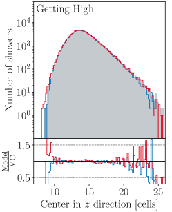
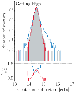
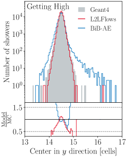
Figure 10: Center of gravity in longitudinal (left), $x$ (middle), and $y$ (left) direction for GettingHigh.

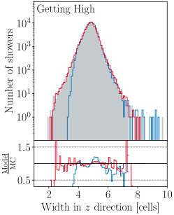
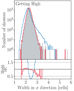
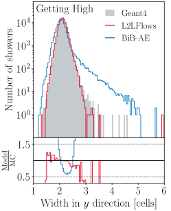
Figure 11: Standard deviation of the energy weighted distributions of longitudinal (left), $x$ (middle), and $y$ (right) positions evaluated on single showers and histogramed over all test showers for GettingHigh.

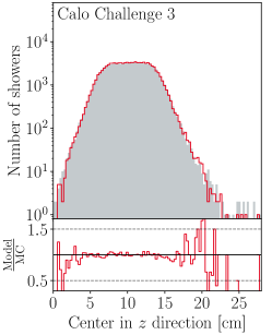
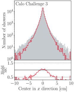
Figure 12: Center of gravity in longitudinal (left), $x$ (middle), and $y$ (left) direction for CaloChallenge 3.

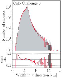
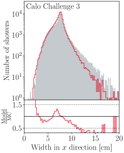
Figure 13: Standard deviation of the energy weighted distributions of longitudinal (left), $x$ (middle), and $y$ (right) positions evaluated on single showers and histogramed over all test showers for CaloChallenge 3.

References

- [1] J. Albrecht et al. (HEP Software Foundation) 2019 A Roadmap for HEP Software and Computing R&D for the 2020s Comput. Softw. Big Sci. 3 7. e-Print: 1712.06982 doi: 10.1007/s41781-018-0018-8
- [2] A. Boehnlein, C. Biscarat, A. Bressan, D. Britton, R. Bolton, F. Gaede, C. Grandi, F. Hernandez, T. Kuhr, G. Merino, F. Simon and G. Watts 2022 HL-LHC Software and Computing Review Panel, 2nd Report Tech. rep. CERN Geneva URL: http://cds.cern.ch/record/2803119
- [3] M. Paganini, L. de Oliveira and B. Nachman 2018 Accelerating Science with Generative Adversarial Networks: An Application to 3D Particle Showers in Multilayer Calorimeters Phys. Rev. Lett. 120 042003. e-Print: 1705.02355 doi: 10.1103/PhysRevLett.120.042003
- [4] M. Paganini, L. de Oliveira and B. Nachman 2018 CaloGAN : Simulating 3D high energy particle showers in multilayer electromagnetic calorimeters with generative adversarial networks Phys. Rev. D 97 014021. e-Print: 1712.10321 doi: 10.1103/PhysRevD.97.014021
- [5] L. de Oliveira, M. Paganini and B. Nachman 2018 Controlling Physical Attributes in GAN-Accelerated Simulation of Electromagnetic Calorimeters J. Phys. Conf. Ser. 1085 042017. e-Print: 1711.08813 doi: 10.1088/1742-6596/1085/4/042017
- [6] M. Erdmann, L. Geiger, J. Glombitza and D. Schmidt 2018 Generating and refining particle detector simulations using the Wasserstein distance in adversarial networks Comput. Softw. Big Sci. 2 4. e-Print: 1802.03325 doi: 10.1007/s41781-018-0008-x
- [7] M. Erdmann, J. Glombitza and T. Quast 2019 Precise simulation of electromagnetic calorimeter showers using a Wasserstein Generative Adversarial Network Comput. Softw. Big Sci. 3 4. e-Print: 1807.01954 doi: 10.1007/s41781-018-0019-7
- [8] D. Belayneh et al. 2020 Calorimetry with deep learning: particle simulation and reconstruction for collider physics Eur. Phys. J. C 80 688. e-Print: 1912.06794 doi: 10.1140/epjc/s10052-020-8251-9
- [9] A. Butter, S. Diefenbacher, G. Kasieczka, B. Nachman and T. Plehn 2021 GANplifying event samples SciPost Phys. 10 139. e-Print: 2008.06545 doi: 10.21468/SciPostPhys.10.6.139
- [10] 2020 Fast simulation of the ATLAS calorimeter system with Generative Adversarial Networks Tech. Rep. ATL-SOFT-PUB-2020-006 CERN Geneva URL: http://cds.cern.ch/record/2746032
- [11] F. Carminati, A. Gheata, G. Khattak, P. Mendez Lorenzo, S. Sharan and S. Vallecorsa 2018 Three dimensional Generative Adversarial Networks for fast simulation J. Phys. Conf. Ser. 1085 032016 doi: 10.1088/1742-6596/1085/3/032016
- [12] P. Musella and F. Pandolfi 2018 Fast and Accurate Simulation of Particle Detectors Using Generative Adversarial Networks Comput. Softw. Big Sci. 2 8. e-Print: 1805.00850 doi: 10.1007/s41781-018-0015-y
- [13] G. Aad et al. (ATLAS) 2024 Deep Generative Models for Fast Photon Shower Simulation in ATLAS Comput. Softw. Big Sci. 8 7. e-Print: 2210.06204 doi: 10.1007/s41781-023-00106-9
- [14] A. Ghosh (ATLAS) 2020 Deep generative models for fast shower simulation in ATLAS J. Phys. Conf. Ser. 1525 012077 doi: 10.1088/1742-6596/1525/1/012077
- [15] G. Aad et al. (ATLAS) 2022 AtlFast3: The Next Generation of Fast Simulation in ATLAS Comput. Softw. Big Sci. 6 7. e-Print: 2109.02551 doi: 10.1007/s41781-021-00079-7
- [16] B. Hashemi, N. Hartmann, S. Sharifzadeh, J. Kahn and T. Kuhr 2023 Ultra-High-Resolution Detector Simulation with Intra-Event Aware GAN and Self-Supervised Relational Reasoning e-Print: 2303.08046
- [17] M. Faucci Giannelli and R. Zhang 2023 CaloShowerGAN, a Generative Adversarial Networks model for fast calorimeter shower simulation e-Print: 2309.06515
- [18] A. Dogru, R. Aydogan, B. Bayrak, S. Ertekin, B. Isildak and E. Simsek 2024 CALPAGAN: Calorimetry for Particles using GANs e-Print: 2401.02248
- [19] E. Buhmann, S. Diefenbacher, E. Eren, F. Gaede, G. Kasieczka, A. Korol and K. Krüger 2021 Getting High: High Fidelity Simulation of High Granularity Calorimeters with High Speed Comput. Softw. Big Sci. 5 13. e-Print: 2005.05334 doi: 10.1007/s41781-021-00056-0
- [20] E. Buhmann, S. Diefenbacher, E. Eren, F. Gaede, G. Kasieczka, A. Korol and K. Krüger 2021 Decoding Photons: Physics in the Latent Space of a BIB-AE Generative Network EPJ Web Conf. 251 03003. e-Print: 2102.12491 doi: 10.1051/epjconf/202125103003
- [21] E. Buhmann, S. Diefenbacher, D. Hundhausen, G. Kasieczka, W. Korcari, E. Eren, F. Gaede, K. Krüger, P. McKeown and L. Rustige 2022 Hadrons, better, faster, stronger Mach. Learn. Sci. Tech. 3 025014. e-Print: 2112.09709 doi: 10.1088/2632-2153/ac7848
- [22] J. C. Cresswell, B. L. Ross, G. Loaiza-Ganem, H. Reyes-Gonzalez, M. Letizia and A. L. Caterini 2022 CaloMan: Fast generation of calorimeter showers with density estimation on learned manifolds 36th Conference on Neural Information Processing Systems: Workshop on Machine Learning and the Physical Sciences. e-Print: 2211.15380
- [23] S. Diefenbacher, E. Eren, F. Gaede, G. Kasieczka, A. Korol, K. Krüger, P. McKeown and L. Rustige 2023 New angles on fast calorimeter shower simulation Mach. Learn. Sci. Tech. 4 035044. e-Print: 2303.18150 doi: 10.1088/2632-2153/acefa9
- [24] S. Hoque, H. Jia, A. Abhishek, M. Fadaie, J. Q. Toledo-Marín, T. Vale, R. G. Melko, M. Swiatlowski and W. T. Fedorko 2023 CaloQVAE : Simulating high-energy particle-calorimeter interactions using hybrid quantum-classical generative models e-Print: 2312.03179
- [25] S. Bieringer, A. Butter, S. Diefenbacher, E. Eren, F. Gaede, D. Hundhausen, G. Kasieczka, B. Nachman, T. Plehn and M. Trabs 2022 Calomplification — the power of generative calorimeter models JINST 17 P09028. e-Print: 2202.07352 doi: 10.1088/1748-0221/17/09/P09028
- [26] Q. Liu, C. Shimmin, X. Liu, E. Shlizerman, S. Li and S.-C. Hsu 2024 Calo-VQ: Vector-Quantized Two-Stage Generative Model in Calorimeter Simulation e-Print: 2405.06605
- [27] C. Krause and D. Shih 2023 Fast and accurate simulations of calorimeter showers with normalizing flows Phys. Rev. D 107 113003. e-Print: 2106.05285 doi: 10.1103/PhysRevD.107.113003
- [28] C. Krause and D. Shih 2023 Accelerating accurate simulations of calorimeter showers with normalizing flows and probability density distillation Phys. Rev. D 107 113004. e-Print: 2110.11377 doi: 10.1103/PhysRevD.107.113004
- [29] S. Schnake, D. Krücker and K. Borras 2022 Generating Calorimeter Showers as Point Clouds Machine Learning and the Physical Sciences, Workshop at the 36th conference on Neural Information Processing Systems (NeurIPS) URL: https://ml4physicalsciences.github.io/2022/files/NeurIPS_ML4PS_2022_77.pdf
- [30] C. Krause, I. Pang and D. Shih 2024 CaloFlow for CaloChallenge Dataset 1 SciPost Phys. 16 126. e-Print: 2210.14245 doi: 10.21468/SciPostPhys.16.5.126
- [31] S. Diefenbacher, E. Eren, F. Gaede, G. Kasieczka, C. Krause, I. Shekhzadeh and D. Shih 2023 L2LFlows: generating high-fidelity 3D calorimeter images JINST 18 P10017. e-Print: 2302.11594 doi: 10.1088/1748-0221/18/10/P10017
- [32] A. Xu, S. Han, X. Ju and H. Wang 2024 Generative machine learning for detector response modeling with a conditional normalizing flow JINST 19 P02003. e-Print: 2303.10148 doi: 10.1088/1748-0221/19/02/P02003
- [33] M. R. Buckley, C. Krause, I. Pang and D. Shih 2024 Inductive simulation of calorimeter showers with normalizing flows Phys. Rev. D 109 033006. e-Print: 2305.11934 doi: 10.1103/PhysRevD.109.033006
- [34] I. Pang, D. Shih and J. A. Raine 2024 SuperCalo: Calorimeter shower super-resolution Phys. Rev. D 109 092009. e-Print: 2308.11700 doi: 10.1103/PhysRevD.109.092009
- [35] F. Ernst, L. Favaro, C. Krause, T. Plehn and D. Shih 2023 Normalizing Flows for High-Dimensional Detector Simulations e-Print: 2312.09290
- [36] S. Schnake, D. Krücker and K. Borras 2024 CaloPointFlow II Generating Calorimeter Showers as Point Clouds e-Print: 2403.15782
- [37] H. Du, C. Krause, V. Mikuni, B. Nachman, I. Pang and D. Shih 2024 Unifying Simulation and Inference with Normalizing Flows e-Print: 2404.18992
- [38] V. Mikuni and B. Nachman 2022 Score-based generative models for calorimeter shower simulation Phys. Rev. D 106 092009. e-Print: 2206.11898 doi: 10.1103/PhysRevD.106.092009
- [39] E. Buhmann, S. Diefenbacher, E. Eren, F. Gaede, G. Kasieczka, A. Korol, W. Korcari, K. Krüger and P. McKeown 2023 CaloClouds: fast geometry-independent highly-granular calorimeter simulation JINST 18 P11025. e-Print: 2305.04847 doi: 10.1088/1748-0221/18/11/P11025
- [40] F. T. Acosta, V. Mikuni, B. Nachman, M. Arratia, B. Karki, R. Milton, P. Karande and A. Angerami 2024 Comparison of point cloud and image-based models for calorimeter fast simulation JINST 19 P05003. e-Print: 2307.04780 doi: 10.1088/1748-0221/19/05/P05003
- [41] V. Mikuni and B. Nachman 2024 CaloScore v2: single-shot calorimeter shower simulation with diffusion models JINST 19 P02001. e-Print: 2308.03847 doi: 10.1088/1748-0221/19/02/P02001
- [42] O. Amram and K. Pedro 2023 Denoising diffusion models with geometry adaptation for high fidelity calorimeter simulation Phys. Rev. D 108 072014. e-Print: 2308.03876 doi: 10.1103/PhysRevD.108.072014
- [43] E. Buhmann, F. Gaede, G. Kasieczka, A. Korol, W. Korcari, K. Krüger and P. McKeown 2024 CaloClouds II: ultra-fast geometry-independent highly-granular calorimeter simulation JINST 19 P04020. e-Print: 2309.05704 doi: 10.1088/1748-0221/19/04/P04020
- [44] E. Buhmann, C. Ewen, D. A. Faroughy, T. Golling, G. Kasieczka, M. Leigh, G. Quétant, J. A. Raine, D. Sengupta and D. Shih 2023 EPiC-ly Fast Particle Cloud Generation with Flow-Matching and Diffusion e-Print: 2310.00049
- [45] C. Jiang, S. Qian and H. Qu 2024 Choose Your Diffusion: Efficient and flexible ways to accelerate the diffusion model in fast high energy physics simulation e-Print: 2401.13162
- [46] D. Kobylianskii, N. Soybelman, E. Dreyer and E. Gross 2024 CaloGraph: Graph-based diffusion model for fast shower generation in calorimeters with irregular geometry e-Print: 2402.11575
- [47] C. Jiang, S. Qian and H. Qu 2024 BUFF: Boosted Decision Tree based Ultra-Fast Flow matching e-Print: 2404.18219
- [48] L. Favaro, A. Ore, S. P. Schweitzer and T. Plehn 2024 CaloDREAM – Detector Response Emulation via Attentive flow Matching e-Print: 2405.09629
- [49] B. Hashemi and C. Krause 2023 Deep Generative Models for Detector Signature Simulation: An Analytical Taxonomy e-Print: 2312.09597
- [50] B. Hashemi, N. Amin, K. Datta, D. Olivito and M. Pierini 2019 LHC analysis-specific datasets with Generative Adversarial Networks e-Print: 1901.05282
- [51] S. Otten, S. Caron, W. de Swart, M. van Beekveld, L. Hendriks, C. van Leeuwen, D. Podareanu, R. Ruiz de Austri and R. Verheyen 2021 Event Generation and Statistical Sampling for Physics with Deep Generative Models and a Density Information Buffer Nature Commun. 12 2985. e-Print: 1901.00875 doi: 10.1038/s41467-021-22616-z
- [52] R. Di Sipio, M. Faucci Giannelli, S. Ketabchi Haghighat and S. Palazzo 2019 DijetGAN: A Generative-Adversarial Network Approach for the Simulation of QCD Dijet Events at the LHC JHEP 08 110. e-Print: 1903.02433 doi: 10.1007/JHEP08(2019)110
- [53] A. Butter, T. Plehn and R. Winterhalder 2019 How to GAN LHC Events SciPost Phys. 7 075. e-Print: 1907.03764 doi: 10.21468/SciPostPhys.7.6.075
- [54] J. Arjona Martínez, T. Q. Nguyen, M. Pierini, M. Spiropulu and J.-R. Vlimant 2020 Particle Generative Adversarial Networks for full-event simulation at the LHC and their application to pileup description J. Phys. Conf. Ser. 1525 012081. e-Print: 1912.02748 doi: 10.1088/1742-6596/1525/1/012081
- [55] Y. Alanazi et al. 2020 Simulation of electron-proton scattering events by a Feature-Augmented and Transformed Generative Adversarial Network (FAT-GAN) e-Print: 2001.11103 doi: 10.24963/ijcai.2021/293
- [56] A. Butter, T. Heimel, S. Hummerich, T. Krebs, T. Plehn, A. Rousselot and S. Vent 2023 Generative networks for precision enthusiasts SciPost Phys. 14 078. e-Print: 2110.13632 doi: 10.21468/SciPostPhys.14.4.078
- [57] A. Butter, N. Huetsch, S. Palacios Schweitzer, T. Plehn, P. Sorrenson and J. Spinner 2023 Jet Diffusion versus JetGPT – Modern Networks for the LHC e-Print: 2305.10475
- [58] J. Spinner, V. Bresó, P. de Haan, T. Plehn, J. Thaler and J. Brehmer 2024 Lorentz-Equivariant Geometric Algebra Transformers for High-Energy Physics e-Print: 2405.14806
- [59] F. Vaselli, F. Cattafesta, P. Asenov and A. Rizzi 2024 End-to-end simulation of particle physics events with Flow Matching and generator Oversampling e-Print: 2402.13684
- [60] J. Bendavid 2017 Efficient Monte Carlo Integration Using Boosted Decision Trees and Generative Deep Neural Networks e-Print: 1707.00028
- [61] M. D. Klimek and M. Perelstein 2020 Neural Network-Based Approach to Phase Space Integration SciPost Phys. 9 053. e-Print: 1810.11509 doi: 10.21468/SciPostPhys.9.4.053
- [62] I.-K. Chen, M. D. Klimek and M. Perelstein 2021 Improved neural network Monte Carlo simulation SciPost Phys. 10 023. e-Print: 2009.07819 doi: 10.21468/SciPostPhys.10.1.023
- [63] C. Gao, J. Isaacson and C. Krause 2020 i-flow: High-dimensional Integration and Sampling with Normalizing Flows Mach. Learn. Sci. Tech. 1 045023. e-Print: 2001.05486 doi: 10.1088/2632-2153/abab62
- [64] E. Bothmann, T. Janßen, M. Knobbe, T. Schmale and S. Schumann 2020 Exploring phase space with Neural Importance Sampling SciPost Phys. 8 069. e-Print: 2001.05478 doi: 10.21468/SciPostPhys.8.4.069
- [65] C. Gao, S. Höche, J. Isaacson, C. Krause and H. Schulz 2020 Event Generation with Normalizing Flows Phys. Rev. D 101 076002. e-Print: 2001.10028 doi: 10.1103/PhysRevD.101.076002
- [66] K. Danziger, T. Janßen, S. Schumann and F. Siegert 2022 Accelerating Monte Carlo event generation – rejection sampling using neural network event-weight estimates SciPost Phys. 12 164. e-Print: 2109.11964 doi: 10.21468/SciPostPhys.12.5.164
- [67] T. Heimel, R. Winterhalder, A. Butter, J. Isaacson, C. Krause, F. Maltoni, O. Mattelaer and T. Plehn 2023 MadNIS - Neural multi-channel importance sampling SciPost Phys. 15 141. e-Print: 2212.06172 doi: 10.21468/SciPostPhys.15.4.141
- [68] T. Janßen, D. Maître, S. Schumann, F. Siegert and H. Truong 2023 Unweighting multijet event generation using factorisation-aware neural networks SciPost Phys. 15 107. e-Print: 2301.13562 doi: 10.21468/SciPostPhys.15.3.107
- [69] E. Bothmann, T. Childers, W. Giele, F. Herren, S. Hoeche, J. Isaacson, M. Knobbe and R. Wang 2023 Efficient phase-space generation for hadron collider event simulation SciPost Phys. 15 169. e-Print: 2302.10449 doi: 10.21468/SciPostPhys.15.4.169
- [70] T. Heimel, N. Huetsch, F. Maltoni, O. Mattelaer, T. Plehn and R. Winterhalder 2023 The MadNIS Reloaded e-Print: 2311.01548
- [71] A. Butter, T. Jezo, M. Klasen, M. Kuschick, S. Palacios Schweitzer and T. Plehn 2023 Kicking it Off(-shell) with Direct Diffusion e-Print: 2311.17175
- [72] L. de Oliveira, M. Paganini and B. Nachman 2017 Learning Particle Physics by Example: Location-Aware Generative Adversarial Networks for Physics Synthesis Comput. Softw. Big Sci. 1 4. e-Print: 1701.05927 doi: 10.1007/s41781-017-0004-6
- [73] A. Andreassen, I. Feige, C. Frye and M. D. Schwartz 2019 JUNIPR: a Framework for Unsupervised Machine Learning in Particle Physics Eur. Phys. J. C 79 102. e-Print: 1804.09720 doi: 10.1140/epjc/s10052-019-6607-9
- [74] E. Bothmann and L. Debbio 2019 Reweighting a parton shower using a neural network: the final-state case JHEP 01 033. e-Print: 1808.07802 doi: 10.1007/JHEP01(2019)033
- [75] K. Dohi 2020 Variational Autoencoders for Jet Simulation e-Print: 2009.04842
- [76] R. Kansal, J. Duarte, H. Su, B. Orzari, T. Tomei, M. Pierini, M. Touranakou, J.-R. Vlimant and D. Gunopulos 2021 Particle Cloud Generation with Message Passing Generative Adversarial Networks 35th Conference on Neural Information Processing Systems. e-Print: 2106.11535
- [77] B. Käch, D. Krücker, I. Melzer-Pellmann, M. Scham, S. Schnake and A. Verney-Provatas 2022 JetFlow: Generating Jets with Conditioned and Mass Constrained Normalising Flows e-Print: 2211.13630
- [78] B. Käch, D. Krücker and I. Melzer-Pellmann 2022 Point Cloud Generation using Transformer Encoders and Normalising Flows e-Print: 2211.13623
- [79] R. Kansal, A. Li, J. Duarte, N. Chernyavskaya, M. Pierini, B. Orzari and T. Tomei 2023 Evaluating generative models in high energy physics Phys. Rev. D 107 076017. e-Print: 2211.10295 doi: 10.1103/PhysRevD.107.076017
- [80] E. Buhmann, G. Kasieczka and J. Thaler 2023 EPiC-GAN: Equivariant point cloud generation for particle jets SciPost Phys. 15 130. e-Print: 2301.08128 doi: 10.21468/SciPostPhys.15.4.130
- [81] M. Leigh, D. Sengupta, G. Quétant, J. A. Raine, K. Zoch and T. Golling 2024 PC-JeDi: Diffusion for particle cloud generation in high energy physics SciPost Phys. 16 018. e-Print: 2303.05376 doi: 10.21468/SciPostPhys.16.1.018
- [82] B. Käch and I. Melzer-Pellmann 2023 Attention to Mean-Fields for Particle Cloud Generation e-Print: 2305.15254
- [83] M. A. W. Scham, D. Krücker and K. Borras 2023 DeepTreeGANv2: Iterative Pooling of Point Clouds e-Print: 2312.00042
- [84] J. Birk, E. Buhmann, C. Ewen, G. Kasieczka and D. Shih 2023 Flow Matching Beyond Kinematics: Generating Jets with Particle-ID and Trajectory Displacement Information e-Print: 2312.00123
- [85] A. Li, V. Krishnamohan, R. Kansal, R. Sen, S. Tsan, Z. Zhang and J. Duarte 2023 Induced Generative Adversarial Particle Transformers 37th Conference on Neural Information Processing Systems. e-Print: 2312.04757
- [86] J. Birk, A. Hallin and G. Kasieczka 2024 OmniJet-: The first cross-task foundation model for particle physics e-Print: 2403.05618
- [87] V. Mikuni and B. Nachman 2024 OmniLearn: A Method to Simultaneously Facilitate All Jet Physics Tasks e-Print: 2404.16091
- [88] P. Ilten, T. Menzo, A. Youssef and J. Zupan 2023 Modeling hadronization using machine learning SciPost Phys. 14 027. e-Print: 2203.04983 doi: 10.21468/SciPostPhys.14.3.027
- [89] A. Ghosh, X. Ju, B. Nachman and A. Siodmok 2022 Towards a deep learning model for hadronization Phys. Rev. D 106 096020. e-Print: 2203.12660 doi: 10.1103/PhysRevD.106.096020
- [90] J. Chan, X. Ju, A. Kania, B. Nachman, V. Sangli and A. Siodmok 2023 Fitting a deep generative hadronization model JHEP 09 084. e-Print: 2305.17169 doi: 10.1007/JHEP09(2023)084
- [91] C. Bierlich, P. Ilten, T. Menzo, S. Mrenna, M. Szewc, M. K. Wilkinson, A. Youssef and J. Zupan 2023 Towards a data-driven model of hadronization using normalizing flows e-Print: 2311.09296
- [92] J. Chan, X. Ju, A. Kania, B. Nachman, V. Sangli and A. Siodmok 2023 Integrating Particle Flavor into Deep Learning Models for Hadronization e-Print: 2312.08453
- [93] B. Nachman and D. Shih 2020 Anomaly Detection with Density Estimation Phys. Rev. D 101 075042. e-Print: 2001.04990 doi: 10.1103/PhysRevD.101.075042
- [94] A. Andreassen, B. Nachman and D. Shih 2020 Simulation Assisted Likelihood-free Anomaly Detection Phys. Rev. D 101 095004. e-Print: 2001.05001 doi: 10.1103/PhysRevD.101.095004
- [95] G. Stein, U. Seljak and B. Dai 2020 Unsupervised in-distribution anomaly detection of new physics through conditional density estimation 34th Conference on Neural Information Processing Systems. e-Print: 2012.11638
- [96] A. Hallin, J. Isaacson, G. Kasieczka, C. Krause, B. Nachman, T. Quadfasel, M. Schlaffer, D. Shih and M. Sommerhalder 2022 Classifying anomalies through outer density estimation Phys. Rev. D 106 055006. e-Print: 2109.00546 doi: 10.1103/PhysRevD.106.055006
- [97] A. Hallin, G. Kasieczka, T. Quadfasel, D. Shih and M. Sommerhalder 2023 Resonant anomaly detection without background sculpting Phys. Rev. D 107 114012. e-Print: 2210.14924 doi: 10.1103/PhysRevD.107.114012
- [98] J. A. Raine, S. Klein, D. Sengupta and T. Golling 2023 CURTAINs for your sliding window: Constructing unobserved regions by transforming adjacent intervals Front. Big Data 6 899345. e-Print: 2203.09470 doi: 10.3389/fdata.2023.899345
- [99] D. Sengupta, S. Klein, J. A. Raine and T. Golling 2023 CURTAINs Flows For Flows: Constructing Unobserved Regions with Maximum Likelihood Estimation e-Print: 2305.04646
- [100] T. Golling, G. Kasieczka, C. Krause, R. Mastandrea, B. Nachman, J. A. Raine, D. Sengupta, D. Shih and M. Sommerhalder 2024 The interplay of machine learning-based resonant anomaly detection methods Eur. Phys. J. C 84 241. e-Print: 2307.11157 doi: 10.1140/epjc/s10052-024-12607-x
- [101] T. Golling, S. Klein, R. Mastandrea and B. Nachman 2023 Flow-enhanced transportation for anomaly detection Phys. Rev. D 107 096025. e-Print: 2212.11285 doi: 10.1103/PhysRevD.107.096025
- [102] G. Bickendorf, M. Drees, G. Kasieczka, C. Krause and D. Shih 2024 Combining resonant and tail-based anomaly detection Phys. Rev. D 109 096031. e-Print: 2309.12918 doi: 10.1103/PhysRevD.109.096031
- [103] E. Buhmann, C. Ewen, G. Kasieczka, V. Mikuni, B. Nachman and D. Shih 2024 Full phase space resonant anomaly detection Phys. Rev. D 109 055015. e-Print: 2310.06897 doi: 10.1103/PhysRevD.109.055015
- [104] D. Sengupta, M. Leigh, J. A. Raine, S. Klein and T. Golling 2024 Improving new physics searches with diffusion models for event observables and jet constituents JHEP 04 109. e-Print: 2312.10130 doi: 10.1007/JHEP04(2024)109
- [105] C. Krause, B. Nachman, I. Pang, D. Shih and Y. Zhu 2023 Anomaly detection with flow-based fast calorimeter simulators e-Print: 2312.11618
- [106] A. Gandrakota, L. Zhang, A. Puli, K. Cranmer, J. Ngadiuba, R. Ranganath and N. Tran 2024 Robust Anomaly Detection for Particle Physics Using Multi-Background Representation Learning e-Print: 2401.08777
- [107] S. Agostinelli, J. Allison, K. Amako, J. Apostolakis, H. Araujo, P. Arce, M. Asai, D. Axen, S. Banerjee, G. Barrand, F. Behner, L. Bellagamba et al. 2003 Geant4—a simulation toolkit Nuclear Instruments and Methods in Physics Research Section A: Accelerators, Spectrometers, Detectors and Associated Equipment 506 250–303 doi: https://doi.org/10.1016/S0168-9002(03)01368-8
- [108] J. Allison, K. Amako, J. Apostolakis, H. Araujo, P. Arce Dubois, M. Asai, G. Barrand, R. Capra, S. Chauvie, R. Chytracek, G. Cirrone, G. Cooperman et al. 2006 Geant4 developments and applications IEEE Transactions on Nuclear Science 53 270–278 doi: 10.1109/TNS.2006.869826
- [109] J. Allison, K. Amako, J. Apostolakis, P. Arce, M. Asai, T. Aso, E. Bagli, A. Bagulya, S. Banerjee, G. Barrand, B. Beck, A. Bogdanov et al. 2016 Recent developments in Geant4 Nuclear Instruments and Methods in Physics Research Section A: Accelerators, Spectrometers, Detectors and Associated Equipment 835 186–225 doi: https://doi.org/10.1016/j.nima.2016.06.125
- [110] O. Ronneberger, P. Fischer and T. Brox 2015 U-Net: Convolutional Networks for Biomedical Image Segmentation Medical Image Computing and Computer-Assisted Intervention (MICCAI) (LNCS vol 9351) (Springer) pp 234–241. e-Print: 1505.04597 doi: 10.1007/978-3-319-24574-4_28
- [111] L. Dinh, D. Krueger and Y. Bengio 2014 NICE: Non-linear Independent Components Estimation. e-Print: 1410.8516
- [112] L. Dinh, J. Sohl-Dickstein and S. Bengio 2016 Density estimation using Real NVP e-Print: 1605.08803
- [113] D. P. Kingma and P. Dhariwal 2018 Glow: Generative Flow with Invertible 1x1 Convolutions Advances in Neural Information Processing Systems vol 31 edited by S. Bengio, H. Wallach, H. Larochelle, K. Grauman, N. Cesa-Bianchi and R. Garnett (Curran Associates, Inc.). e-Print: 1807.03039
- [114] C. Durkan, A. Bekasov, I. Murray and G. Papamakarios 2019 Neural Spline Flows Advances in Neural Information Processing Systems edited by H. Wallach, H. Larochelle, A. Beygelzimer, F. Alché-Buc, E. Fox and R. Garnett (Curran Associates, Inc.). e-Print: 1906.04032
- [115] M. Faucci Giannelli, G. Kasieczka, B. Nachman, D. Salamani, D. Shih and A. Zaborowska 2022 Fast Calorimeter Simulation Challenge 2022 GitHub page URL: https://github.com/CaloChallenge/homepage
- [116] H. Abramowicz et al. (ILD Concept Group) 2020 International Large Detector: Interim Design Report e-Print: 2003.01116
- [117] M. A. Thomson 2009 Particle Flow Calorimetry and the PandoraPFA Algorithm Nucl. Instrum. Meth. A 611 25–40. e-Print: 0907.3577 doi: 10.1016/j.nima.2009.09.009
- [118] 2016 iLCSoft Project Page URL: https://github.com/iLCSoft
- [119] M. Frank, F. Gaede, C. Grefe and P. Mato 2014 DD4hep: A Detector Description Toolkit for High Energy Physics Experiments J. Phys. Conf. Ser. 513 022010 doi: 10.1088/1742-6596/513/2/022010
- [120] M. F. Giannelli, G. Kasieczka, C. Krause, B. Nachman, D. Salamani, D. Shih and A. Zaborowska 2023 Fast Calorimeter Simulation Challenge 2022 - Dataset 1 Version 3 doi: 10.5281/zenodo.8099322
- [121] M. F. Giannelli, G. Kasieczka, C. Krause, B. Nachman, D. Salamani, D. Shih and A. Zaborowska 2022 Fast Calorimeter Simulation Challenge 2022 - Dataset 2 doi: 10.5281/zenodo.6366271
- [122] M. F. Giannelli, G. Kasieczka, C. Krause, B. Nachman, D. Salamani, D. Shih and A. Zaborowska 2022 Fast Calorimeter Simulation Challenge 2022 - Dataset 3 doi: 10.5281/zenodo.6366324
- [123] Par04 example URL: https://gitlab.cern.ch/geant4/geant4/-/tree/master/examples/extended/parameterisations/Par04
- [124] D. J. Rezende and S. Mohamed 2015 Variational Inference with Normalizing Flows International conference on machine learning (PMLR) pp 1530–1538. e-Print: 1505.05770
- [125] I. Kobyzev, S. J. D. Prince and M. A. Brubaker 2021 Normalizing Flows: An Introduction and Review of Current Methods IEEE Trans. Pattern Anal. Machine Intell. 43 3964–3979. e-Print: 1908.09257 doi: 10.1109/tpami.2020.2992934
- [126] G. Papamakarios, E. Nalisnick, D. J. Rezende, S. Mohamed and B. Lakshminarayanan 2021 Normalizing Flows for Probabilistic Modeling and Inference J. Machine Learning Res. 22 2617–2680. e-Print: 1912.02762 doi: 10.5555/3546258.3546315
- [127] M. Germain, K. Gregor, I. Murray and H. Larochelle 2015 MADE: Masked Autoencoder for Distribution Estimation e-Print: 1502.03509
- [128] G. Papamakarios, T. Pavlakou and I. Murray 2017 Masked Autoregressive Flow for Density Estimation e-Print: 1705.07057
- [129] A. Paszke, S. Gross, F. Massa, A. Lerer, J. Bradbury, G. Chanan, T. Killeen, Z. Lin, N. Gimelshein, L. Antiga, A. Desmaison, A. Kopf et al. 2019 PyTorch: An Imperative Style, High-Performance Deep Learning Library Advances in Neural Information Processing Systems 32 edited by H. Wallach, H. Larochelle, A. Beygelzimer, F. d’Alché Buc, E. Fox and R. Garnett (Curran Associates, Inc.) pp 8024–8035 URL: http://papers.neurips.cc/paper/9015-pytorch-an-imperative-style-high-performance-deep-learning-library.pdf
- [130] C. Durkan, A. Bekasov, I. Murray and G. Papamakarios 2020 nflows: normalizing flows in PyTorch Zenodo doi: 10.5281/zenodo.4296287
- [131] D. P. Kingma and J. Ba 2014 A Method for Stochastic Optimization. e-Print: 1412.6980
- [132] S. Park, D. Han and N. Kwak 2021 The U-Net based GLOW for Optical-Flow-free Video Interframe Generation. e-Print: 2103.09576
- [133] L. N. Smith and N. Topin 2018 Super-Convergence: Very Fast Training of Neural Networks Using Large Learning Rates. e-Print: 1708.07120
- [134] I. Loshchilov and F. Hutter 2017 Decoupled Weight Decay Regularization International Conference on Learning Representations. e-Print: 1711.05101
- [135] A. Niculescu-Mizil and R. Caruana 2005 Predicting good probabilities with supervised learning Proceedings of the 22nd international conference on Machine learning pp 625–632 doi: 10.1145/1102351.1102430