Scattering and dynamical capture of two black holes: synergies between numerical and analytical methods

Abstract

We study initially unbound systems of two black holes using numerical relativity (NR) simulations performed with GR-Athena++. We focus on regions of the parameter space close to the transition from scatterings to dynamical captures, considering equal mass and spin-aligned configurations, as well as unequal mass and nonspinning ones. The numerical results are then used to validate the effective-one-body (EOB) model TEOBResumS-Dalí for dynamical captures and scatterings. We find good agreement for the waveform phenomenologies, scattering angles, mismatches, and energetics in the low energy regime ($E_{0}\lesssim 1.02\,M$). In particular, mismatches are typically below or around the $1\%$ level, with only a few cases – corresponding to spinning binaries – slightly above the $3\%$ threshold. We also discuss dynamical captures in the test-mass limit by solving numerically the Zerilli equation with the time domain code RWZHyp. The latter analysis provides valuable insights into both the analytical noncircular corrections of the EOB waveform and the integration of NR Weyl scalars.

I Introduction

With the experimental advancements in gravitational wave (GW) observatories and the development of new data analysis techniques by the LIGO-Virgo-KAGRA (LVK) collaboration Abbott et al. (2019, 2021a, 2021b), GW astronomy has become a standard tool to explore the universe. This prompts the necessity to provide accurate descriptions of the dynamics of astrophysical compact binaries, which are the sources of all the GW signals detected so far. This urgency is amplified by the high sensitivity that will be reached with next-generation detectors, such as Einstein Telescope Punturo et al. (2010); Maggiore et al. (2020), Cosmic Explorer Reitze et al. (2019) and LISA Amaro-Seoane et al. (2017). Although the majority of compact binaries circularize by the time their gravitational signals enter the sensitivity band of our detectors Peters and Mathews (1963), certain dense astrophysical environments, such as globular clusters, can host compact two-body systems with elliptic or hyperbolic-like orbits Samsing et al. (2014); Rodriguez et al. (2016); Belczynski et al. (2016); Samsing (2018); Rodriguez et al. (2018); Mukherjee et al. (2020); Dall’Amico et al. (2021, 2024). The event GW190521 might have been precisely generated by a black hole binary (BBH) of this nature Romero-Shaw et al. (2020); Gayathri et al. (2022); Gamba et al. (2023).

In this work we focus on initially unbound two-black-hole systems. Configurations of this kind can become bound due to dissipative effects linked to the emission of GWs, ultimately leading to the merger of the two objects. Such systems are known as dynamical captures. Crucially, depending on the energy and angular momentum considered, the dynamically captured black holes can undergo many highly eccentric orbits before merging. On the other hand, if the GW emission due to the mutual interaction is not strong enough to make the system bound, the two compact objects will simply scatter. The transition from scatterings to captures is particularly delicate to study, since small variations in the initial data can lead to very different phenomenologies Gold and Brügmann (2013). This aspect is particularly relevant if these systems are studied numerically, since numerical relativity (NR) simulations are computationally expensive, and the outcome of the simulation cannot be easily predicted by just looking at the initial data. It is therefore preferable to also have (semi-)analytical models that can quickly provide predictions on the phenomenologies of these systems. Analytical methods that have been proved to be successful in describing coalescing BBHs include the post-Newtonian (PN) Einstein et al. (1938); Einstein and Infeld (1940); Blanchet and Damour (1989); Damour et al. (2014a); Schaefer and Jaranowski (2018) and post-Minkowskian (PM) Bel et al. (1981); Damour (2016); Bern et al. (2019); Damour (2020); Dlapa et al. (2023) frameworks, whose synergies are essential to build effective-one-body (EOB) models Buonanno and Damour (1999, 2000); Damour et al. (2000); Buonanno et al. (2007); Nagar et al. (2007); Damour and Nagar (2007); Damour et al. (2009, 2013); Nagar et al. (2018); Cotesta et al. (2018); Pompili et al. (2023); Nagar et al. (2023). In this work we consider the last avatar of TEOBResumS-Dalí Nagar et al. (2024), a PN-based EOB model that has been already used to study both elliptic and hyperbolic systems, providing reliable results despite being numerically informed only on quasi-circular NR simulations Chiaramello and Nagar (2020); Nagar et al. (2021a, b); Albanesi et al. (2021); Nagar and Rettegno (2021); Placidi et al. (2022); Albanesi et al. (2022a, b); Bonino et al. (2023); Hopper et al. (2023); Nagar et al. (2023); Andrade et al. (2024); Nagar et al. (2024). Since the model is based on PN-approximate results, numerical data for generic orbits are also needed for its validation. The interplay between analytical and numerical methods in studying BBHs is indeed well-established, and it is therefore not surprising that this synergy retains its importance also for initially unbound orbits, where its relevance may even be heightened. We thus explore the hyperbolic regime close to the scattering-capture transition by performing NR simulations with GR-Athena++ Daszuta et al. (2021); Cook et al. (2023). After surveying the parameter space and highlighting the challenges encountered, we compare the numerical and analytical results. We also study the metric perturbations generated by dynamical captures in the test-mass limit, that are governed by the Regge-Wheeler and Zerilli (RWZ) equations with a test particle source term Regge and Wheeler (1957); Zerilli (1970); Nagar and Rezzolla (2005); Martel and Poisson (2005). In particular, we solve the Zerilli equation by means of the time-domain code RWZHyp Bernuzzi and Nagar (2010); Bernuzzi et al. (2011a, 2012). These waveforms can be employed to assess the reliability of the EOB analytical prescriptions in a more controlled environment, as well as to elucidate the numerical integration procedures used in the NR case, highlighting any associated systematic issues.

The paper is structured as follows. In Sec. II we present our new numerical simulations: we discuss the initial data in Sec. II.1, the time evolution performed with GR-Athena++ in Sec. II.2, and the post-processing in Sec. II.3. The phenomenologies are examinated in Sec. II.4, with a focus on the transition from scattering to capture. Remnant properties for merging configurations are investigated in Sec. II.5. Subsequently, in Sec. III we introduce the EOB model TEOBResumS-Dalí and the comparisons with the numerical results, discussing, in particular: i) the phenomenologies across the parameter space in Sec. III.2, ii) the scattering angles in Sec. III.3, iii) the mismatches in Sec. III.4, and iv) the energetics in Sec. III.5. Finally, in Sec. IV we study the test mass limit, focusing on nonspinning configurations. The dynamics and the relevance of the radiation reaction in this regime are analyzed in Sec. IV.1, while the RWZ numerical perturbations are presented in Sec. IV.2. The latter waveforms are also employed to validate the EOB inspiral waveform in Sec. IV.3. Throughout this paper we use geometrized unit, $G=c=1$.

II Numerical relativity simulations

We begin our survey of the parameter space of initially unbound systems by presenting 84 new NR simulations with varying mass ratios and spins. More precisely, in Sec. II.1 we discuss how we choose the initial data for these runs, that are then time-evolved as described in Sec. II.2. While most of the configurations in this paper correspond to equal mass nonspinning systems, we also simulate some cases with spin and higher mass-ratios. The complete list of simulations considered in this work is shown in Fig. 1 and reported in Tables 3 and 4. In Sec. II.4 we discuss their phenomenologies by means of guage-invariant quantities computed as explained in Sec. II.3.

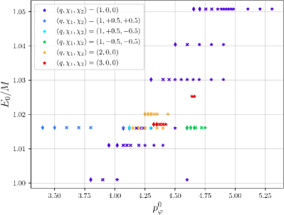
Figure 1: Comparable mass configurations considered in this work. Different markers indicate different phenomenologies: stars for scatterings, diamonds for direct plunges, crosses for double encounters, and a plus for the only triple encounter of our dataset. Colors are related to $(q,\chi_{1},\chi_{2})$ combinations, see legend.

II.1 Initial data

When simulating systems close to the scattering-capture transition, small variations in the initial data can lead to completely different outcomes; it is thus difficult to guess, a priori, the phenomenology. To predict the evolution across the parameter space, we employ the state-of-the-art EOB model TEOBResumS-Dalí Nagar et al. (2021a, b); Nagar and Rettegno (2021); Nagar et al. (2023, 2024). After fixing the initial ADM energy to a value greater than the total rest mass of the system ($E_{0}>M$), we systematically explore various initial orbital angular momenta $L_{0}$ with the EOB model, selecting specific sets that define configurations close to the threshold between scatterings and captures. Note that the EOB prediction is not guaranteed to be fully consistent with the outcome of the numerical simulation, since the model is PN-approximate. This is however not an issue, since we only use TEOBResumS-Dalí to understand which region of the parameter space should be explored with numerical simulations. In practice, we fix $r_{\rm EOB}=100\,M$, and for each pair of values of energy and angular momentum, we compute the corresponding Cartesian EOB initial positions and momenta. We then compute the Cartesian positions and momenta using a 2PN EOB/ADM transformation Buonanno and Damour (1999); Bini and Damour (2012). These quantities are then used to initialize the NR simulation. The energy and the angular momenta have the same values in both ADM and EOB charts, so in terms of $(E,L,r)$, the only quantity that actually needs the 2PN transformation is the initial separation $r$. For the values of energy and angular momentum considered in this work, $r_{\rm EOB}=100\,M$ translates in an ADM separation $D$ that is still close to $100\,M$ (precise values are reported in Tables 3 and 4). While in practice variations of a few units do not drastically change the outcome of the numerical simulation, since the GW emission at these large separations is indeed small, we still employ the transformation to compute $D$ to be as consistent as possible.

The reliability of the EOB/ADM transformation can be tested by comparing the initial ADM energy and angular momentum of the simulation with the original values used in the EOB chart. As anticipated, they should be equal, but given the finite PN-accuracy of the transformation, this is not guaranteed. As expected, the agreement tends to decrease for higher initial velocities due to the PN approximation employed in the coordinate transformation. For example, for an initial EOB energy $1.011\,M$, the relative difference with the corresponding ADM energy at the beginning of the numerical simulation is $3\cdot 10^{-5}$; for initial energy $1.050\,M$ this relative difference grows to $8\cdot 10^{-4}$.

The Cartesian momenta and separation are used together with the individual black hole spins to initialize a stand-alone version of the thorn TwoPunctures Brandt and Brügmann (1997); Ansorg et al. (2004); Daszuta et al. (2021). The total rest mass of the system is computed as $M=M_{1}+M_{2}$, where $M_{i}$ are the ADM masses of the punctures as defined in Eq. (83) of Ref. Ansorg et al. (2004); we choose $M_{1}>M_{2}$ and $M=1$ for all the configurations considered. The mass ratio is denoted as $q=M_{1}/M_{2}$. We always consider systems whose spins are (anti-)aligned with the orbital angular momentum, so that the only non vanishing component of the spin vectors is the $z$ one, simply denoted as $S_{i}$, or with its dimensionless counterpart, $\chi_{i}\equiv S_{i}/M_{i}^{2}$. The total angular momentum of the system is given by $J=L+S_{1}+S_{2}$. It is convenient to also define the reduced angular momentum $j\equiv J/(\nu M^{2})$ and the canonical orbital angular momentum $p_{\varphi}\equiv L/(\nu M^{2})$, where $\nu=q/(q+1)^{2}$ is the symmetric mass ratio. We often use the dimensionless energy defined by $\hat{E}\equiv E/M$.

When reporting the NR initial data, we do not remove the contribution of the junk radiation. We checked that the relative differences in energy and angular momentum before and after junk radiation are below the $10^{-4}$ threshold, and they are thus negligible for the purposes of this work. The junk contributions are estimated from the waveform and the corresponding integrated energy and angular momentum fluxes evaluated at $t=200\,M$, computed as detailed in Sec. II.3.1 and II.3.2. Similar small values were also found for scattering configurations with initial separation $D=100\,M$ in Ref. Damour et al. (2014b), where the waveform and the fluxes where computed with time domain integration.

II.2 Numerical methods

Given some initial data prescribed as discussed in the previous section, we perform the time evolution by means of GR-Athena++ Daszuta et al. (2021); Cook et al. (2023), that employs the Z4c formulation of the Einstein field equations Bernuzzi and Hilditch (2010); Ruiz et al. (2011); Weyhausen et al. (2012); Hilditch et al. (2013). For these new runs, we employ the same moving puncture gauge conditions and gauge parameters as those used in Refs. Daszuta et al. (2021); Andrade et al. (2024). Further, similarly to the GR-Athena++ runs considered in Ref. Andrade et al. (2024), we employ 6th order finite-difference methods for the spatial derivatives, and a 8th order Kreiss-Oliger operator, but with dissipation factor $\epsilon=0.1$. For the time-integration, we use a 4th order Runge-Kutta algorithm and a Courant-Friedrichs-Lewy factor of 0.25. The typical edge of the grid considered is $L=3072\,M$. Different choices have also been explored, without finding any substantial difference in the results. We evolve only the $z>0$ portion of the space and we complete the rest of the grid exploiting bitant symmetry.

GR-Athena++ utilizes an oct-tree structure, with the grid initially organized as a mesh divided into meshblocks. These meshblocks have the same number of grid points, but may differ in physical size. In the case of a cubic initial mesh and cubic meshblocks, three parameters govern the grid setup: the number of grid points on the edges of the unrefined initial mesh $N_{M}$, the number of grid points on the edges of meshblocks $N_{B}$, and the number of physical refinement levels $N_{L}$. The grid structure is ultimately dictated by an adaptive mesh refinement (AMR) criterion. When satisfied, this criterion (de)refines a given MeshBlock, resulting in a smaller or larger block with double or half the resolution, respectively. For these simulations we consider the AMR criterion with $L_{2}$-norm as described in Ref. Rashti et al. (2024). In all of the simulations considered in this work, we use $N_{B}=16$, while we choose $N_{L}$ according to the mass-ratio. More specifically, we typically use $N_{L}=\{11,12,13\}$ for $q=\{1,2,3\}$, respectively. Finally, we use different values for $N_{M}$ depending on the configuration considered, typically $N_{M}=\{128,192,256\}$. The resolution at punctures $\delta x_{p}$ is given by Eq. (40) of Ref. Daszuta et al. (2021). The information on the runs is summarized in Tables 3 and 4, where we report the information for the highest resolution of each physical configuration analyzed in this work.

II.3 Post-processing

In this section we address the computation of gauge-invariant quantities derived from the numerical simulations previously discussed. In particular, we examine gravitational waveforms, energetics, remnant properties, and scattering angles.

II.3.1 Numerical waveforms

During the numerical time-evolution of the system, GR-Athena++ extracts the Weyl scalar $\psi_{4}$ at finite distance integrating over discrete 2-spheres with geodesic grids Daszuta et al. (2021) and different radii. The $2\%$ discrepancy in the GR-Athena++ amplitude that was observed in previous comparisons with other NR codes Daszuta et al. (2021); Andrade et al. (2024) has now been fixed. The Weyl scalar for each extraction radius $R$ is then decomposed in multipoles using the spin-weighted spherical harmonics ${}_{-2}Y_{{\ell m}}(\Theta,\Phi)$. We consider $R=100\,M$, if not specified otherwise. The gravitational strain is also decomposed on the same basis,

$$h_{+}-ih_{\times}=D_{L}^{-1}\sum_{\ell=2}\sum_{m=-\ell}^{\ell}{}_{-2}Y_{{\ell m}}(\Theta,\Phi)h_{\ell m},$$ (1)

where $D_{L}$ is the luminosity distance, and the waveform multipoles $h_{\ell m}$ are related to the Weyl scalar by the asymptotic relation

$$\ddot{h}_{\ell m}=\psi_{4}^{{\ell m}}.$$ (2)

Since we are interested in the waveform at infinity, we need to extrapolate $\psi_{4}^{\ell m}$ before performing the double-time integration. We thus apply the procedure proposed in Refs. Lousto et al. (2010); Nakano et al. (2015); Nakano (2015); Daszuta et al. (2021),

$$\lim_{r\rightarrow\infty}r\psi_{4}^{\ell m}\simeq A\bigg{(}\bar{r}\psi_{4}^{\ell m}-\frac{(\ell-1)(\ell+2)}{2\bar{r}}\int dt\,\bar{r}\psi_{4}^{\ell m}\bigg{)}\,,$$ (3)

where $A=1-2M/\bar{r}$ is the Schwarzschild metric potential, and $\bar{r}=R(1+M/(2R))^{2}$ is the areal radius. This quantity is also used to compute the tortoise coordinate

$$\bar{r}_{*}=\bar{r}+2M\log\left(\frac{\bar{r}}{2M}-1\right)\,,$$ (4)

and the retarded time $u\equiv t-\bar{r}_{*}$. From the extrapolated scalar, obtaining $h_{\ell m}$ appears straightforward at a first glance. It is however well-known that the presence of numerical noise can induce drifts in the signal Reisswig and Pollney (2011), making the integration not trivial. The standard procedure used in the quasi-circular case is the fixed frequency integration (FFI), that consists in performing a frequency-domain integration with a low-frequency cut-off $f_{0}$ Reisswig and Pollney (2011). Clearly, if $f_{0}$ is too low, the unphysical drifts are not removed from the waveform. In the quasi-circular or eccentric cases, the physical range of frequencies is finite, and a cut-off frequency below the lowest physical frequency is typically enough to remove the noise-generated drifts, without cutting-off physical contributions. However, for highly-eccentric configurations, the waveform frequency at apastron $\omega_{\rm ap}$ can be so low that a cut-off $f_{0}<\omega_{\rm ap}$ does not yield reliable waveforms. The situation is even more delicate for hyperbolic-like orbit, where the frequency spectrum is not bounded. As a consequence, for highly non-circular configurations, the FFI inevitably removes physical contributions from the waveform. For this reason, direct time-domain integration (TDI) is in principle preferable. However, as mentioned before, a direct TDI can lead to evident drifts. A typical solution to overcome this problem is to remove the drift, after each integration step, with a polynomial fit (typically linear or constant), that is usually performed only on the last portion of the signal. However, this method can lead to unreliable waveforms for some configurations, especially for signal with long time durations, such as dynamically-bounded binaries with multiple encounters. For this reason, in this work we decide to use the FFI with $f_{0}=0.007M^{-1}$ for all the equal mass cases, and $f_{0}=0.010M^{-1}$ for the unequal mass ones, even if this procedure inevitably removes the low-frequency part of waveforms. In particular, the portion of the waveform generated when the two black holes are farther apart will be strongly suppressed.

The drifts caused by the numerical noise are not the only ones present in highly non-circular waveforms, since the motion of the punctures towards the extraction zone can lead to drifts in $\psi_{4}^{\ell m}$. While this could be in principle cured by just considering farther extraction zones, waveforms extracted at large radii are negatively impacted by numerical dissipation. This issue is particularly relevant for bounded configurations with large apastra and scatterings. Higher mass ratios make the problem even worse. This drift in the scattering case affects both TDI and FFI integrations: in the first case this drift spoils the late-time fit, while in the latter having a non-periodic $\psi_{4}^{\ell m}$ can induce spectral leakage due to the fast Fourier transform used. However, the latter issue can be easily solved by applying time-windows that artificially send the initial and last portions of the signal to zero. The windowing is particularly relevant for the last part of scattering waveforms.

We conclude by mentioning that, for some configurations, we also consider Cauchy Characteristic Extraction (CCE). We dumped the metric quantity needed for the characteristic extraction, that was then performed as post-processing step employing the public code PITTNull Bishop et al. (1998); Babiuc et al. (2011). Comparisons between extrapolated finite-distance and CCE waveforms are reported in Appendix A, where we argue that improved high-pass frequency filters should be considered in future works. For this reason, in the main body of this work we use waveforms extracted at finite distance and then extrapolated according to Eq. (3).

II.3.2 Energetics

In our analysis, it is crucial to accurately differentiate between scattering events and captures. Visual inspection of the punctures’ tracks can be misleading, as it is challenging to distinguish, within the simulation time, proper scatterings from systems that will merge in the distant future. The most reliable method to differentiate these outcomes is to examine the energy after the first encounter, when the two black holes have reached a reasonable large separation. If the energy satisfies the condition $E<M$, the two objects will inevitably merge; otherwise, they will scatter. The energetics are thus a fundamental tool in our analysis.

These curves can be computed once that the waveform has been extracted. The energy and angular momentum instantaneous fluxes are indeed given by

$$\dot{E} =\frac{1}{16\pi}\sum_{\ell=2}\sum_{m=-\ell}^{\ell}|\dot{h}_{{\ell m}}|^{2},$$ (5a)

$$\dot{J} =-\frac{1}{16\pi}\sum_{\ell=2}\sum_{m=-\ell}^{\ell}m\Im\left(\dot{h}_{{\ell m}}h_{{\ell m}}^{*}\right),$$ (5b)

where the asterisk denotes a complex conjugation and $\Im$ is the imaginary part operator. In this work we consider all the multipoles up to $\ell=5$. Note that $\dot{E}$ involves only the News $\dot{h}_{{\ell m}}$, while the computation of $\dot{J}$ also requires the strain. As a consequence, energy fluxes are more accurate than angular momentum ones, since they require one fewer integration step. We can then integrate Eqs. (5) and compute the total energy and angular momentum radiated by the system as a function of time. We can then subtract these quantities to the initial values $(E_{0},J_{0})$ and obtain the time-evolution of the energy and angular momentum, $E(t)$ and $J(t)$. We can then calculate the reduced binding energy

$$\hat{E}_{b}=\frac{E(t)-M}{\mu},$$ (6)

where $\mu=\nu M$ is the reduced mass of the system. Finally, combining the binding energy with the reduced angular momentum $j=J/(\nu M^{2})$, we obtain the gauge-invariant energetic curves $\hat{E}_{b}(j)$.

In the case of coalescing binaries, the energetic curves can be used to estimate the properties of the remnant. Indeed, balance equations imply that the mass $M_{f}$ and spin $a_{f}$ of the remnant are given by the final values of energy and angular momentum.

II.3.3 Scattering angles

In the case of systems with final positive binding energy, we can compute the gauge-invariant scattering angle by extrapolating the tracks of the black holes Damour et al. (2014b). More precisely, we convert the relative motion of the two punctures in polar coordinates $(r,\varphi)$, and we extrapolate the incoming and outgoing trajectories, $\varphi_{\rm in}(r)$ and $\varphi_{\rm out}(r)$, using $1/r$-polynomials. The constant terms of the two polynomials give the asymptotic incoming and outgoing angles, $\varphi_{\rm in}^{\infty}$ and $\varphi_{\rm out}^{\infty}$, that can be used to compute the scattering angle

$$\chi\equiv\varphi_{\rm out}^{\infty}-\varphi_{\rm in}^{\infty}-\pi.$$ (7)

The portions of the tracks that we consider for the fits are $r\in[25,80]\,M$ and $r\in[25\,M,r_{f}]$, for the ingoing and outgoing motion, respectively. Here $r_{f}$ is the separation reached by the two punctures at the end of the simulation. For the ingoing part, we consider an initial radius that is smaller than the initial separation; this is due to the fact that the two punctures have zero initial velocities. Similar to previous works Damour et al. (2014b); Hopper et al. (2023); Damour and Rettegno (2023); Rettegno et al. (2023), the polynomial extrapolation is performed with a least-squares fitting method that uses a singular-value decomposition (SVD). Singular values smaller than $10^{-13}$ times the maximum singular value are dropped. Typically, with the aforementioned SVD, the angle tends to plateau around polynomial order $n=6$, yielding consistent values for higher orders; this resulting value is assigned to $\chi$. The error associated to this extrapolation is computed as the difference between the highest and lowest angles obtained with the different polynomial extrapolations, i.e., $\Delta\chi_{\rm fit}=\chi_{n}^{\rm max}-\chi_{n}^{\rm min}$.

Another source of error is the finite resolution employed in the simulations. We test the relevance of this error for a few scattering configurations by considering two resolutions, $N_{M}=\{128,256\}$. We then compute the error $\Delta\chi_{\rm res}$ as the difference between the two angles obtained. However, for all the cases considered we find $\Delta\chi_{\rm res}<0.3{}^{\circ}$, while $\Delta\chi_{\rm fit}\sim 1-3^{\circ}$. Since the total error is computed as a square sum of the individual errors, $\Delta\chi_{\rm res}$ is in practice negligible. We thus considered most of the scattering configurations at resolution $N_{M}=128$, assigning to each of them a conservative resolution error $\Delta\chi_{\rm res}=0.3^{\circ}$.

We conclude this discussion by recalling that the velocities of the punctures are strictly linked to the shift vector $\beta^{i}$ Campanelli et al. (2006). Since the tracks are gauge-dependent quantities, one should pay extra care when using them to compute the gauge-invariant scattering angle. While the relevance of the initial value for the lapse function $\alpha$ has been tested in Ref. Rettegno et al. (2023), tests on the Gamma-driver, and thus on $\beta_{i}$, should be performed to precisely quantify the relevance of the gauge-choices on the numerical scattering angle. However, a remarkable agreement between the numerical and the analytical agreement has been found in many works Damour et al. (2014b); Hopper et al. (2023); Damour and Rettegno (2023); Rettegno et al. (2023) for most configurations, leading us to think, a posteriori, that the effects of the gauge choices are indeed small, at least for the energy range considered.

II.4 Phenomenology

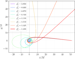
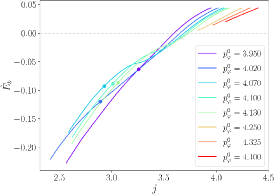
Figure 2: Scatterings and dynamical captures for equal mass systems with fixed initial energy $E_{0}\simeq 1.011\,M$ and different initial angular momenta $p_{\varphi}^{0}$; the latter are reported in the legends. We show the tracks of one puncture, the extrapolated (2,2) Weyl scalars, and the energetics. The circles in the $\hat{E}_{b}(j)$ curves mark the time of the merger, defined as the last peak of the (2,2) waveform amplitude (see Appendix C for more details). The horizontal line in the right panel marks the parabolic limit.

As anticipated, initially unbound systems can have a rich variety of phenomenologies. If the gravitational wave emission is not strong enough to make the system bound, then the two black holes will simply scatter. However, if enough radiation is emitted, then the system becomes bound and the two black holes are doomed to merge. The latter scenario can happen in essentially two situations, which correspond to different regions of the orbital parameter space, i.e. the $(p_{\varphi},E)$ plane. The first situation occurs when the system has a relatively low angular momentum or, equivalently, when the impact parameter $b=L/|p|$ is rather small, being $|p|$ the modulus of the linear momentum. In this case, the two black holes pass closer to each other, prompting a significant emission of radiation. The two black holes can either merge at their first encounter (direct captures), or they may initially rebound, only to complete a single orbit and ultimately merge during the subsequent close encounter. We denote the latter systems as double encounters. The second situation instead occurs when the initial energy is slightly above the parabolic limit $\hat{E}_{b}=0$. In this case, even a small interaction can produce enough gravitational waves to bind the two black holes, that can undergo many encounters before merging, as long as enough angular momentum is provided. These two regions of the parameter space are visualized for the equal mass nonspinning case in Fig. 8, were we considered both numerical simulations and analytical predictions. This figure will be further discussed in Sec. III

II.4.1 Nonspinning equal mass systems

We study the equal mass nonspinning case by considering several values of energy. For each of them, we examine different angular momenta that result in scattering events, double encounters, and direct captures. We start by discussing eight simulations with fixed initial energy $E_{0}\simeq 1.011\,M$ and initial separation $D\simeq 102.8\,M$. We report the tracks of the punctures in the left panel of Fig. 2, while in the middle panel of the same figure we show $\psi_{22}^{4}$ extrapolated to infinity through Eq. (3). In the right panel we draw the energetic curves $\hat{E}_{b}(j)$, also highlighting the merger time, which is defined as the last peak of the (2,2) waveform amplitude. It is crucial to consider the last peak of the amplitude rather than the highest one, since the latter might occur during encounters that do not promptly result in a coalescence; see Appendix C for more detail.

The three configurations with higher initial canonical angular momentum, $p_{\varphi}^{0}\simeq\{4.400,4.325,4.250\}$, are scatterings. As the initial angular momentum is decreased, the gravitational emission at the first encounter is enhanced and the systems become bound. For $p_{\varphi}^{0}\simeq\{4.130,4.100,4.070\}$, the trajectories diverge after the first encounter, gradually increasing the separation between the two black holes. However, upon reaching the apastron –the point of maximum separation– they begin to move towards each other again and eventually merge. As a consequence, the Weyl scalar clearly exhibits two amplitude peaks. For $p_{\varphi}^{0}\simeq 4.020$, the two punctures perform a quasi-circular whirl before plunging and merging; this dynamics still produces two close peaks in the Weyl scalar, but no outgoing motion of the punctures is observed. Moreover, these two peaks unify after integration, thus becoming indistinguishable in the strain. We thus classify this event as a direct capture. Finally, the configuration with lowest angular momentum, $p_{\varphi}^{0}\simeq 3.950$, also results in a direct capture.

We also mention that we evolve a configuration with same initial energy and $p_{\varphi}^{0}\simeq 4.200$, that is not shown in Fig. 2. The reason for this choice is that, after the first encounter, the system becomes bound ($E\sim 0.999\,M$ after the first encounter), but we did not complete the simulation till merger. However, knowing that this configuration is bound allows us to put a more stringent bound on the interval in which the transition from scattering to dynamical capture occurs. Indeed, with this information, we can claim that, at fixed initial energy $E_{0}\simeq 1.011\,M$, this transition occurs for a canonical angular momentum $p_{\varphi}^{0}$ in the interval $\left[4.200,4.250\right]$, where the first value corresponds to the capture with highest simulated $p_{\varphi}^{0}$, and the second one corresponds to the scattering with lowest angular momentum. We thus identify the angular momentum at which the transition occurs as $p_{\varphi}^{*}=4.225\pm 0.025$.

We repeat this analysis for different energies, considering in total five values in the range $E_{0}\in[1.011,1.051]\,M$. The corresponding $p_{\varphi}^{*}$, with associated error bars, are reported in Fig. 3. In the same figure, we also report the fit of the scattering-merger transition recently proposed in Ref. Kankani and McWilliams (2024) (red). The latter is performed using energies up to $E=1.1\,M$, and assuming the ansatz

$$p_{\varphi}^{*}(\hat{E})=\frac{a\hat{E}^{2}+b\hat{E}+c}{\hat{E}-1},$$ (8)

where the coefficients are $(a_{K},b_{K},c_{K})=(15.4932,-27.0216,11.5292)$ (note that here we use $p_{\varphi}$ rather than $L$, so that the coefficients of Ref. Kankani and McWilliams (2024) are $\nu$-rescaled here). We use our simulations to perform a similar fit. However, our five datapoints approximately lay on a line, so that regressing them using the ansatz of Eq. (8) would provide a fit that could not be safely extrapolated to higher energies (gray in Fig. 3). While a linear fit is a more natural choice (blue in Fig. 3), the linear regression would certainly fail for energies close to the parabolic limit. We thus proceed as follows: i) we perform a linear fit, ii) we fix the $a$-parameter of Eq. (8) with the angular coefficient found with the linear regression, iii) we fit the two remaining parameters, $\{b,c\}$, using the ansatz Eq. (8). The final result is shown in orange in Fig. 3, together with the corresponding $95\%$ confidence interval. While our fit and, in particular, the quadratic coefficient $a=15.37\pm 0.81$, are compatible with the results of Ref. Kankani and McWilliams (2024), our scattering-merger transition is systematically shifted at slightly higher angular momenta for $E\gtrsim 1.01$. Moreover, the fit proposed by the authors of Ref. Kankani and McWilliams (2024) predicts $p_{\varphi}^{*}=4.767$ for $\hat{E}=1.05079$, the highest energy considered in this work, while from our numerical data we have $p_{\varphi}^{*}=4.830\pm 0.025$. The small discrepancies might be linked to the different methods employed to compute the fluxes from $\psi_{4}$, that are used to estimate the energy after the first encounter, i.e. the quantity that dictates the final state of the system (bound or unbound). Indeed, Ref. Kankani and McWilliams (2024) uses, for initially unbound configurations, a time-domain integration for $\psi_{4}$ extracted at $R=140\,M$, while we use an FFI applied to the Weyl scalar extracted at $R=100\,M$. Number of multipoles considered and resolutions employed might also play a role in this discrepancy. Finally, notice that our simulations start from an initial separation $D\sim 100\,M$, while the ones considered in Ref. Kankani and McWilliams (2024) start from $D=60\,M$, where the effects of the junk radiation might be more relevant. However, the fit of Ref. Kankani and McWilliams (2024) lays within our $95\%$ confidence interval.

We conclude this discussion by remarking that we also run a series of simulations at initial energy $E_{0}=1.001\,M$. However, since the fate of the configuration with highest orbital angular momentum ($p_{\varphi}^{0}\simeq 4.600$) is not clear and the other three configurations are captures, we do not employ these data in our fit. The uncertainties on the final state are linked to the fact that different integration options lead to different energies after the first close passage, some of them being slightly below the parabolic limit, and others slightly above. In Figs. 1 and 8, we label this simulation as a scattering, basing the decision on our default integration setting. However, this classification should be interpreted with caution.

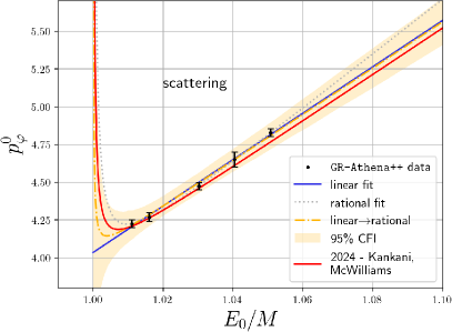
Figure 3: Canonical initial angular momentum that marks the transition from scattering to bound systems as a function of energy for $(q,\chi_{1},\chi_{2})=(1,0,0)$. We show the data points obtained from the GR-Athena++ simulations (black), together with different fits (see text for more details).

II.4.2 Spinning equal mass systems

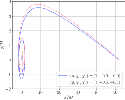
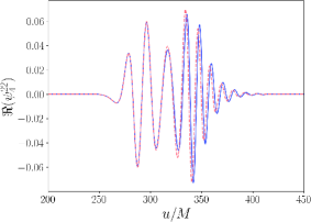
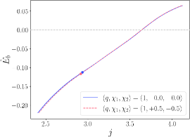
Figure 4: Tracks of one puncture, extrapolated Weyl scalars, and energetic curves for equal mass configurations with same initial separation, same angular momentum $p_{\varphi}^{0}=4.12001$, and same energy $E_{0}\simeq 1.016$ (within the $\sim 0.01\%$ level), but different spin configurations (solid blue for the nonspinnig case, dashed red for $\chi_{1}=-\chi_{2}=0.5$). The circles in the energetics mark the merger time. The two configurations are rather similar as predicted by PN theory, since the leading order spin-orbit contribution is vanishing for equal mass binaries with anti-aligned individual spins.

We now turn our attentions to equal mass systems with aligned and anti-aligned spins. We consider spins with magnitude $|\chi_{i}|=0.5$ and different orientations.

We start by studying configurations whose individual spins have opposite signs. According to PN theory, the main spin correction vanishes for equal mass binaries with this spin configuration Racine (2008); Santamaria et al. (2010). We thus expect the phenomenology of systems with anti-aligned individual spins to be quite similar to the nonspinning case. An explicit example for dynamical capture described within the EOB formalism is reported in Fig. 6 of Ref. Nagar et al. (2021a) (see also Fig. 7 therein).

In order to verify this prediction, we consider a spinning configuration with $(q,\chi_{1},\chi_{2})=(1,+0.5,-0.5)$ and $(\hat{E}_{0},p^{0}_{\varphi})=(1.01619,4.12001)$. The corresponding Weyl scalar and energetic curve are then compared against a nonspinning configuration with equivalent orbital parameters in Fig. 4. The initial energy in the latter case is $E_{0}=1.01607\,M$, with a $\sim 0.01\%$ discrepancy with respect to the spinning case. The tracks of the punctures reported in the left panel of Fig. 4 show that these two configurations have a quasi-circular whirl before the plunge. While the corresponding (2,2) waveforms are initially well aligned ($|\Delta\phi|\lesssim 0.015$ radians for retarded time $u<300\,M$), the dephasing rapidly increases afterward, finally saturating at $|\Delta\phi|\sim 1$ radian for $u=350\,M$. This discrepancy in the phase is also clearly visible in the Weyl scalar reported in the middle panel of Fig. 4. Since dephasing occurs only after $u=300\,M$, we are prone to think that this phase difference is linked to higher-order spin contributions rather than to the $0.01\%$ discrepancy in the initial energies. Indeed, significant differences in initial energies would influence the timing of the close encounter, causing a misalignment throughout the entire waveforms. A similar conclusion can be also drawn by inspecting the energetic curves.

The analysis is repeated also for a larger angular momentum, $p_{\varphi}^{0}\simeq 4.300$, which results in scattering in both the spinning and non-spinning configurations. In this case, the comparison between the waveforms is even more striking, since no evident dephasing is observed for the whole evolution ($|\Delta\phi|\lesssim 0.015$ radians up to the close encounter, reaching at most $|\Delta\phi|\sim 0.06$ radians afterwards). The result is not surprising since, as illustrated in Fig. 4 for $p_{\varphi}^{0}\simeq 4.120$, there is no evidence of strong dephasing in the waveform generated at the first close encounter; instead, the dephasing becomes more pronounced during the quasi-circular whirl that occurs just before the plunge. Despite a visual discrepancy in the gauge-dependent tracks of the punctures for $p_{\varphi}^{0}\simeq 4.120$ (that can be observed also for the previous case, as shown in the left panel of Fig. 4), the scattering angles are perfectly compatible, since they are $301.5\pm 1.7{}^{\circ}$ and $303.6\pm 2.0{}^{\circ}$ for the nonspinning and spinning cases, respectively. These results, together with the ones for $p_{\varphi}^{0}\simeq 4.120$, confirm the prediction of Ref. Nagar et al. (2021a).

We now move to the case in which both spins are anti-aligned with the orbital angular momentum, $\chi_{1}=\chi_{2}=-0.5$. In heuristic terms, the frame dragging of the two black holes opposes to the orbital motion, so that, in order to avoid captures, we need to provide more orbital angular momentum (or, equivalently, higher impact parameters). We thus simulate an energy series with $E_{0}=1.01619\,M$ and angular momenta $p_{\varphi}^{0}\in[4.600,4.750]$. The dominant multipoles of $\psi_{4}$ and the energetics computed with all the multipoles up to $\ell=5$ are shown in the left panels of Fig. 5. For the configuration with $p_{\varphi}^{0}\simeq 4.720$, we have a double encounter where the two black holes merge at $u\sim 3115\,M$. This very long simulation poses different challenges to the integration process. First of all, consider that the maximum separation reached after the first encounter is $D_{\rm ap}\sim 100\,M$, meaning that the two punctures have an outgoing motion up to a grid radius of $R\sim 50\,M$. This motion generates visible drifts in the waveform extracted at radii $R\lesssim 120\,M$, that become negligible only for higher extraction radii. Note that this issue might occur also for scatterings, if the outgoing motion is evolved long enough. However, this problematic behaviour can be easily fixed, at least for the cases investigated in this work, by considering larger extraction radius; we thus consider $R=140\,M$ for this double encounter. Secondly, the long duration of the signal makes time-domain integration impracticable; even considering higher-order polynomials to remove the accumulated drift does not produce meaningful strains. On the contrary, FFI methods produce more reliable waveform once that the aforementioned issue with the outgoing motion is solved.

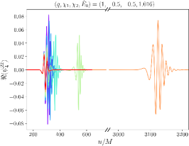
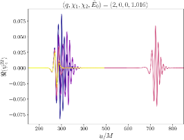
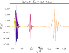
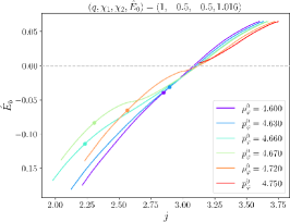
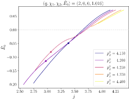
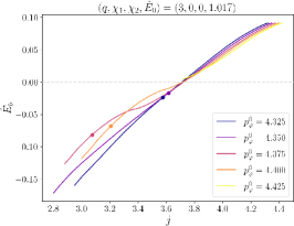
Figure 5: Real parts of $\psi_{4}^{22}$ and energetic curves for an equal mass energy series with $\chi_{i}=-0.5$ (left) and two energy series for unequal mass nonspinning configurations. The markers in the energetics highlight the merger time. The angular momenta are shown in the legends of the bottom panels.

For the energy considered ($E_{0}=1.01619\,M$), we find that the transition from scattering to captures occurs for $p_{\varphi}^{*}=4.735\pm 0.015$. In the nonspinning case, for a very similar energy ($E_{0}=1.01607\,M$) we got $p_{\varphi}^{*}=4.270\pm 0.030$. The nonspinning value is smaller than the spinning one, as expected. The larger error in the nonspinning case is only linked to the sampling of the parameter space; more targeted simulations would easily reduce the uncertainties.

We repeat this analysis at the same energy, but for aligned spins, namely $\chi_{1}=\chi_{2}=0.5$. We find that the transition from scattering to dynamical capture occurs at $p_{\varphi}^{*}=3.935\pm 0.035$, i.e. at a lower orbital angular momentum with respect to the anti-aligned and nonspinning cases, as a priori expected.

II.4.3 Nonspinning unequal mass systems

Finally, we discuss nonspinning configurations with higher mass ratios. These configurations are more computationally expensive, since more resolution has to be employed in order to correctly resolve the punctures. For this reason, we just focus on a few significant cases, and leave a more systematic exploration to future work. We consider three scattering-capture transitions at fixed energy, specifically $E_{0}\simeq\{1.016,1.020\}\,M$ for $q=2$, and $E_{0}\simeq 1.017\,M$ for $q=3$. We further consider two spinning configurations with $q=3$ and $E_{0}\simeq 1.025$.

The (2,2) extrapolated Weyl scalars and the energetics for two series are reported in the middle and right panels of Fig. 5. The long duration of the $q=3$ configuration with $p_{\varphi}^{0}\simeq 4.400$ poses integration issues that are similar to the ones discussed in the previous section. Also in this case, considering $\psi_{4}$ extracted at $140\,M$ fixes the problems. The transition from scattering to captures occurs at $p_{\varphi}^{*}=4.300\pm 0.050$ for $q=2$ and $E\simeq 1.016\,M$, and at $p_{\varphi}^{*}=4.410\pm 0.012$ for $q=3$ and $E\simeq 1.017\,M$. We recall that the width of the errors on $p_{\varphi}^{*}$ is just linked to the sampling of the parameter space, and not to physical uncertainties. The values obtained for these configurations are similar to the equal mass nonspinning case, showing that the impact of the mass-ratio on the scattering-capture threshold is smaller than the one related to the spin.

II.5 Properties of the remnants

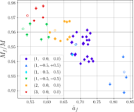
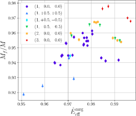
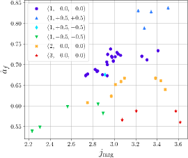
Figure 6: First panel: masses and spins of remnants generated by dynamical captures (filled markers). We also report the values for quasi-circular mergers as given by the fits of Ref. Jiménez-Forteza et al. (2017); Nagar et al. (2020) (empty circles). Middle and right panels: remnant masses and spins plotted against the effective energy $\hat{E}_{\rm eff}$ and the $\nu$-rescaled angular momentum $j$, respectively. Both quantities on the $x$-axise are evaluated at merger. In the legends we report $(q,\chi_{1},\chi_{2})$.

We now discuss the properties of the remnants for coalescing configurations. The corresponding masses and spins are reported in Tables 3 and 4, and shown in Fig. 6, where each color/marker type highlight a different $(q,\chi_{1},\chi_{2})$-combination. We also report, for reference, the quasi-circular values obtained from the post-merger fits of Refs. Jiménez-Forteza et al. (2017); Nagar et al. (2020) (empty circles).

Similarly to the quasi-circular case, the individual black hole spins strongly influence the properties of the remnant. Following Ref. Carullo et al. (2024), we plot the spins and the masses against the $\nu$-rescaled angular momentum $j$ and the effective energy $\hat{E}_{\rm eff}$, respectively. Both quantities are evaluated at the merger time $t_{\rm mrg}$. The effective energy $\hat{E}_{\rm eff}$ is defined according to the usual effective-one-body map Buonanno and Damour (1999),

$$\hat{E}_{\rm eff}=1+\frac{\hat{E}^{2}-1}{2\nu}.$$ (9)

It is important to note that, in the test-mass limit, $\hat{E}$ reduces to the total rest mass of the system, while $\hat{E}_{\rm eff}$ becomes the energy of the particle; we come back to the (nonspinning) test-particle limit in Sec. IV. To evaluate $j$ and $\hat{E}_{\rm eff}$ at merger, we integrate the angular momentum and energy fluxes up to $t_{\rm mrg}$ and remove the radiated fluxes from the initial values $(J_{0},E_{0})$; then $(j_{\rm mrg},\hat{E}_{\rm eff}^{\rm mrg})$ are computed accordingly. We recall, in passing, that the description of the main post-merger features for non-circular BBHs can be achieved by considering the gauge-invariant dynamical impact parameter $\hat{b}_{\rm mrg}$, as discussed in Refs. Albanesi et al. (2023); Carullo et al. (2024).

Binaries whose individual spins are anti-aligned with the orbital angular momentum produce heavier and slower-rotating remnants than binaries with nonspinning progenitors. The opposite occurs for spin-aligned binaries, where the remnants are lighter and faster-rotating. This scaling can be understood as follows. Progenitors with aligned spins ($\chi_{i}>0$) tend to have more stable orbits, and therefore spend more time at small separations. They thus emit a larger amount of radiation, and ultimately produce less massive and faster-rotating remnants. On the contrary, the plunge starts at larger separations for binaries with anti-aligned spins ($\chi_{i}<0$), so that the two black holes spend less time close to each other. As a consequence, the system emits less gravitational radiation, generating a more massive and slower-rotating remnant. A similar scaling is also observed for quasi-circular BBHs, where nonspinning progenitors lead to $M_{f}=0.952\,M$ and $\hat{a}_{f}=0.686$, while $\chi_{i}=0.5$ ($-0.5$) leads to $M_{f}=0.933\,M$ (0.962) and $\hat{a}_{f}=0.831$ (0.527) Jiménez-Forteza et al. (2017); Nagar et al. (2020).

Finally, we examine the impact of the finite resolution and the integration procedure on the remnant properties. We start by considering the energetics for all the physical configurations that have been run both at $N_{M}=128$ and $N_{M}=256$. We then compute the differences between the remnant properties found at the two resolutions, finding that the highest absolute differences among equal mass binaries occur for the nonspinning configuration with $(\hat{E}_{0},p_{\varphi}^{0})\simeq(1.051,4.654)$, and correspond to $(\Delta\hat{M}_{f},\Delta\hat{a}_{f})=(0.0013,0.0036)$, where $\hat{M}_{f}=M_{f}/M$. If we also consider the nonspinning unequal mass binaries, the maximum differences are $\Delta M_{f}=0.0014\,M$ and $\Delta\hat{a}_{f}=0.0048$, and occur for the $q=3$ configuration with $(\hat{E}_{0},\,p_{\varphi}^{0})\simeq(1.017,4.398)$. For all the configurations that have been run only at one resolution, we conservatively assign errors equal to the maximum differences found in our dataset.

To evaluate the error linked to the integration procedure, we consider a configuration that can be safely integrated both in the time and frequency domains. We examine the case with $(\hat{E}_{0},p_{\varphi}^{0})\simeq(1.011,3.950)$, obtaining $(\hat{M}_{f}^{\rm TDI},\hat{a}_{f}^{\rm TDI})=(0.9417,0.6351)$ and $(\hat{M}_{f}^{\rm FFI},\hat{a}_{f}^{\rm FFI})=(0.9432,0.6409)$, so that the absolute differences are $(\Delta\hat{M}_{f},\Delta\hat{a}_{f})=(0.0015,0.0058)$. Note than these errors are slightly larger that the maximum discrepancies associated to the resolution.

The total error on the remnant properties is finally computed as the square root of the quadrature sum of the resolution and integration errors; they are shown in in Fig. 6, and also reported in Tables 3 and 4.

III Accuracy of EOB models for scatterings and dynamical captures

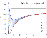
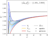
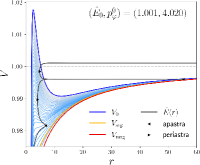
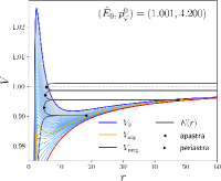
Figure 7: Time evolution of effective EOB potentials $V(r;p_{\varphi})$ for different physical configurations with $\hat{E}_{0}=1.001$. From left to right, we have a direct capture, followed by a double encounter, a triple encounter, and finally, a quadruple encounter. The evolution of the energy $\hat{E}$ (dark gray) is overlapped to radial potentials (blue shades). We highlight the initial potential (dark blue), the potential at the separatrix-crossing (orange), and the potential at merger (red). We also mark apastra and periastra, when defined. The first apastron of the quadruple encounter is not shown for graphical reasons, since it occurs at $r\sim 172$.

Numerical relativity stands as the golden standard for generating accurate waveforms for compact binaries. However, exploring large parameter spaces, as the one studied in this work, is extremely expensive from the computational point of view. Herein lies the advantage of (semi-)analytical methods, that offer a more manageable approach, albeit at the cost of introducing analytical approximations. Furthermore, these methods often incorporate calibrations performed on quasi-circular binaries. Therefore, to ensure the region of validity of analytical models, it is necessary to assess their reliability through comparisons with NR simulations. In this paper we consider the EOB framework, and in particular we test the reliability of the TEOBResumS-Dalí model Nagar et al. (2023, 2024) in the scattering and dynamical capture scenarios. Previous versions of this model have been already tested for these kind of configurations in Refs. Damour et al. (2014b); Gamba et al. (2023); Hopper et al. (2023); Damour and Rettegno (2023); Andrade et al. (2024), but here we extend this analysis by considering a larger portion of the orbital parameter space, and focusing on the transition from scattering to plunge. We also mention that series of scattering configurations at fixed energy could be used to test PM predictions Damour and Rettegno (2023); Rettegno et al. (2023), but we do not carry out this analysis here, since the energies for the scatterings considered in this work are similar to the ones analyzed in Ref. Rettegno et al. (2023) (see Table I therein).

III.1 Effective-one-body model

For a complete and up-to-date description of TEOBResumS-Dalí, we point to Refs. Chiaramello and Nagar (2020); Nagar et al. (2023, 2024). Here we describe the most relevant aspects for our analysis. The basic idea of EOB models is to map the two-body problem into the motion of a single particle that moves in an effective metric. This metric is a $\nu$-deformation of Schwarzschild or Kerr, depending on whether the spins of the black holes are vanishing or not. The map is created by encoding the conservative PN equations of motion in an EOB Hamiltonian Buonanno and Damour (1999); Damour (2001). State-of-the-art EOB model use 5PN-accurate Hamiltonians, which are completed with numerically-informed coefficients. In particular, TEOBResumS-Dalí includes two free effective coefficients, $a_{6}$ and $c_{3}$, that are informed by nonspinning and spinning NR simulations, respectively Nagar et al. (2023, 2024). This calibration is performed on quasi-circular waveforms of the SXS catalog SXS ; Buchman et al. (2012); Chu et al. (2009); Hemberger et al. (2013); Scheel et al. (2015); Blackman et al. (2015); Lovelace et al. (2012, 2011); Mroue et al. (2013); Lovelace et al. (2015); Kumar et al. (2015); Lovelace et al. (2016); Chu et al. (2016); Varma et al. (2019). The dissipative effects due to gravitational wave emission, that starts from 2.5PN, are taken into account including in the Hamilton’s equation a radiation reaction force obtained through energy-balance equations Bini and Damour (2012). Note that TEOBResumS-Dalí consider the quasi-circular limit of radial radiation reaction valid for generic orbits. The angular component of the radiation reaction is the standard quasi-circular prescription of TEOBResumS-Giotto, dressed with a generic quadrupolar Newtonian prefactor Chiaramello and Nagar (2020), which generalizes ${\cal F}_{\varphi}$ to generic planar orbits. The reliability of these prescriptions have been extensively tested, both in the test-mass limit and in the comparable mass case Chiaramello and Nagar (2020); Albanesi et al. (2021, 2022a); Nagar et al. (2023). The EOB dynamics is then obtained solving the corresponding Hamilton’s equations. While analytical methods are available for early quasi-circular inspirals Nagar and Rettegno (2019), these equations have to be solved numerically for quasi-circular late inspirals or elliptic/hyperbolic-like orbits. The EOB dynamics is then used to compute the multipolar waveform at infinity.

Each multipole of the analytical inspiral waveform includes a generic Newtonian prefactor. We further discuss the inspiral EOB waveform used in TEOBResumS-Dalí in Sec. IV.3. The analytical wave is then completed with a ringdown model, that describes the waveform generated after the merger of the two black holes. The smooth match between the inspiral and ringdown waveforms is typically achieved through Next-to-Quasi-Circular (NQC) corrections. Both the ringdown model and the NQC corrections in TEOBResumS-Dalí are based on quasi-circular NR simulations. For this reason, in this work we switch-off the NQC corrections, as done in the analysis of GW190521 Abbott et al. (2020) performed in Ref. Gamba et al. (2023).

As anticipated, our goal is to test the reliability of TEOBResumS-Dalí for scatterings and dynamical captures, without incorporating numerical non-circular information into the semi-analytical model. However, the merger-ringdown waveform could be improved considering numerical simulations of highly eccentric binaries and dynamical captures Andrade et al. (2024); Carullo et al. (2024). The enhancement of the conservative sector via numerical information should also be studied, but no calibration on NR simulations with generic orbits has been achieved so far. Both generalizations are left to future works.

As typically done in the EOB literature, we consider rescaled EOB phase space variable $(r,p_{r_{*}},\varphi,p_{\varphi})$, which are related to the physical ones by $r=R/M$, $p_{r_{*}}=P_{r_{*}}/\mu$, and $p_{\varphi}=P_{\varphi}/(\mu M)$. The latter variable has been already extensively used in this work.

III.2 Orbital parameter space

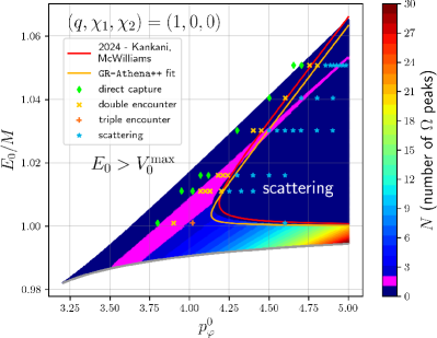
Figure 8: Phenomenologies of equal mass nonspinning systems across the parameter space. The colormap highlight the number of peaks of the orbital frequency $N$, that is a proxy of the number of encounters, as predicted by TEOBResumS-Dalí. Quasi-circular binaries are highlighted with a gray line. The NR simulations considered in this work are reported with markers and colors that correspond to different phenomenologies. We also show the scattering-capture fits discussed in Sec. II.4.1.

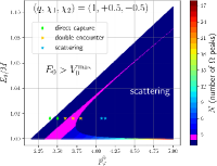
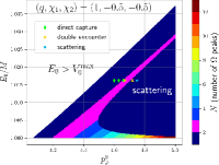
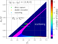
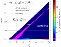
Figure 9: Phenomenologies for different $(q,\chi_{1},\chi_{2})$ configurations; analogous to Fig. 8, but only for initially unbound orbits. The colormap highlights the number of orbital frequency peaks as predicted by TEOBResumS-Dalí, while the markers correspond to the numerical simulations. Note the different vertical scales.

An extensive exploration of the parameter space can be easily achieved with semi-analytical models that are able to generate hundreds of waveforms in less than a second on conventional consumer-grade computing machines. Such an exploration for initially unbound configurations has been performed in Ref. Nagar et al. (2021a) for nonspinnig systems with different mass ratios. However, the reliability of these predictions has to be checked using computationally expensive NR simulations.

We consider both bound and unbound initial data, examining pairs of energy and angular momentum that satisfy $V_{\rm min}^{0}\leq E_{0}\leq V_{\rm max}^{0}$, where $V_{\rm min}^{0}$ ($V_{\rm max}^{0}$) is the minimum (maximum) of the initial EOB radial potential $V(r;p_{\varphi})$. The latter is defined by setting to zero the radial momentum in the EOB Hamiltonian,

$$V(r;p_{\varphi})\equiv H_{\rm EOB}(r,p_{\varphi},p_{r_{*}}=0).$$ (10)

The condition $E_{0}=V_{\rm min}^{0}$ thus identifies stable circular orbits, that slowly evolve under the effects of the radiation reaction; configurations with smaller energies are not allowed. On the other hand, orbital configurations with $E_{0}>V_{\rm max}^{0}$ can occur, but in this case we aprioristically know that we will have a direct capture. We thus focus on initial energies that lie between the initial minimum and maximum values of the effective potential.

Since GWs are emitted, the system loses angular momentum, causing the effective potential $V(r;p_{\varphi})$ to change over time. Analyzing the evolution of this potential provides valuable insights into the dynamics of the system, as already shown, for example, in Ref. Albanesi et al. (2023), where test-particles orbiting around Schwarzschild black holes along eccentric orbits were considered. Here, instead, we focus on configurations with comparable masses. The evolutions of energies and effective potentials for four initially unbound, equal mass, nonspinning systems are illustrated in Fig. 7. For all the cases, we consider an energy slightly above the parabolic limit, $\hat{E}_{0}=1.001$, and select the angular momenta in order to obtain a direct capture and configurations with two, three and four encounters. Note that first three configurations have been also simulated numerically with GR-Athena++. We also highlight the potential at three specific times: at the beginning of the evolution (blue), at the separatrix-crossing (orange), and at merger time (red). The latter quantity is estimated from the peak of the pure orbital frequency (without spin-orbit coupling) as $t_{\rm mrg}^{\rm EOB}=t^{\rm peak}_{\Omega_{\rm orb}}-3$ Nagar et al. (2020). We recall that the separatrix is an eccentric generalization of the last stable orbit O’Shaughnessy (2003); Stein and Warburton (2020), and stable orbits are no longer allowed after the crossing of this quantity; this crossing can be identified, in terms of the potential, as $\hat{E}=V_{\rm max}$. In the case of the direct capture show in Fig. 7 ($p_{\varphi}^{0}=3.800$), enough radiation is emitted to cause the separatrix to be crossed at the first encounter, leading the system to plunge without experiencing any outgoing motion. The other configurations are instead more interesting: the systems still become bound at the first encounter, but conserving the property $\hat{E}<V_{\rm max}$. As a consequence, after the first close encounter we have radial motion confined between the two radial turning points, the apastron and the periastron. As long as the binding energy is negative and $\hat{E}<V_{\rm max}$, these two turning points can be identified at the any time by solving $\hat{E}=V$. Once that the separatrix is crossed, the periastron ceases to exist also for these configurations, leading the two black holes to merge. We conclude the discussion on the effective potentials by mentioning that in the scattering scenario, we simply have a rebound on the (evolving) potential barrier.

We now start to span the equal mass nonspinning parameter space more systematically. For initially unbound configurations, we consider a very large radius at which the influence of the radiation reaction force is completely negligible ($r_{0}=5\cdot 10^{3}$ for practical purposes). For bound configurations, we start the EOB evolution at the apastron, which is uniquely determined by $(E_{0},p_{\varphi}^{0})$. The phenomenology of the waveform can be tracked by looking at the number of peaks of the orbital frequency $\Omega\equiv\dot{\varphi}$, denoted as $N$. Each peak marks a close encounter between the two black holes, so that $N\geq 2$ marks double and multiple encounters, while $N=1$ marks either direct captures or scatterings. The result for the nonspinning equal mass case is reported in Fig. 8 up to $p_{\varphi}^{0}=5$. Quasi-circular configurations are highlighted with a gray line. The region in which we have two encounters (magenta) shrinks as the energy increases, sharpening the transition from scatterings to direct captures. This implies that, according to the analytical prediction, double encounters are more likely to occur for low energies.

On the same figure, we report the numerical results. We show all the equal mass nonspinning configurations considered in this work. The markers and the colors highlight different phenomenologies: direct captures are highlighted with green diamonds, double encounters with yellow crosses, and scatterings with blue stars; the only triple encounter of our dataset is marked with an orange cross. While the NR configurations are started at a smaller separation ($D\sim 100\,M$), than the EOB predictions ($r_{0}=5\cdot 10^{3}$), the effects of the radiation reaction (and the junk radiation) are already negligible at the initial NR separation.

Especially for low energies, the phenomenologies predicted by TEOBResumS-Dalí are in agreement with the corresponding numerical ones. Notably, the EOB model predicts the correct number of close passages also for the triple encounter. However, as we further discuss below, this does not guarantee a low EOB/NR mismatch, since the encounters can occur at rather different times. The reliability of the EOB waveform is further discussed in Sec. III.4.

The disagreement between the EOB prediction and the NR simulations grows as the initial energy increases. In particular, for high energy the NR transition from scattering to merger occurs at lower orbital angular momenta than predicted by the EOB model. This behaviour is better highlighted by the fits of this transition, that have been aready discussed in Sec. II.4.1. It is interesting to observe that the slope of these fits diverges from the double encounter region predicted by the EOB model for high-energy. As a consequence, in the high-energy region of the parameter space, we can have NR scatterings that occur at energies above the maximum of the EOB potential, i.e. with $E_{0}>V^{0}_{\rm max}$. Since the potential is computed from the EOB Hamiltonian $H_{\rm EOB}$, this means that even the solely conservative sector of the EOB model is no longer accurate for high energies. This does not come as a surprise, since $H_{\rm EOB}$ is based on PN results that lose their reliability at high relative velocities. Moreover, the calibration of the effective parameters $a_{6}$ and $c_{3}$ is performed only on quasi-circular binaries. Higher-order PN information or PM results, together with a calibration performed on a wider region of the parameter space, could mitigate this problem. This exploration, which is far from trivial, is left to future work. Moreover, while the aforementioned observation highlight the limitation of the EOB Hamiltonian, also the radiation reaction force is PN-approximate; more accurate fluxes would probably improve the EOB/NR agreement. The interplay between conservative and dissipative sectors require in depth studied, as already highlighted in Ref. Nagar et al. (2024) for initially bound configurations.

We extend this analysis also to the spinning cases with $\chi_{\rm eff}=\pm 0.5$ and to the the nonspinning $q=\{2,3\}$. The corresponding parameter spaces as predicted by TEOBResumS-Dalí, together with the numerical results, are reported in Fig. 9. Even if for these values of $(q,\chi_{1},\chi_{2})$ we have simulated less orbital configurations than for the equal mass nonspinning case, a few considerations can be made. First of all, the numerical simulations confirm that TEOBResumS-Dalí is able to reproduce the phenomenologies of spinning scatterings and dynamical captures, at least for the energies and spins considered. However, one should also notice that the double encounter region ($N=2$, magenta) was captured with a higher accuracy in the nonspinning case (cfr. with Fig. 8). Secondly, the accuracy of the EOB model seems to degrade for higher mass ratios, since all the three $q=3$ scattering configurations are in a region where TEOBResumS-Dalí predicts dynamical captures. However, two of them are at the relatively high energy $E_{0}\simeq 1.025\,M$, and all of them have large scattering angles, $\chi>327^{\circ}$ (see Table 4). The EOB/NR agreement for the $q=2$ case is instead better, and the three corresponding scattering configurations are indeed in the unbound region of TEOBResumS-Dalí. However, in the $q=2$ case, all the scattering angles are below $310^{\circ}$. A more detailed analysis of spinning configurations and unequal mass systems is postponed to future work.

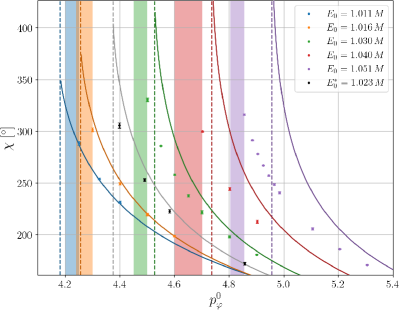
Figure 10: Scattering angles $\chi$ for equal mass nonspinning systems. Different colors highlight different initial energies. Markers and error bars correspond to the GR-Athena++ results. The colored bands highlight the region in which the NR scattering-capture transition occurs. We also report the EOB prediction using lines of the same colors, showing a rather good agreement in the low energy regime $E_{0}\lesssim 1.02$, even for high scattering angles. The vertical dashed lines mark the EOB scattering-capture transition. The NR data for $E_{0}\simeq 1.023\,M$ are taken from Ref. Damour et al. (2014b).

III.3 Nonspinning equal mass scatterings

Table 1: EOB/NR scattering angles for the equal mass nonspinning configurations considered in this work. We also include the configurations of Ref. Damour et al. (2014b) ($E_{0}\simeq 1.023\,M$).

$\hat{E}_{0}$	$p_{\varphi}^{0}$	$\chi_{\rm NR}\pm\Delta\chi_{\rm NR}\,[{}^{\circ}]$	$\chi_{\rm EOB}[{}^{\circ}]$
1.01103	4.24996	$288.4\pm 1.7$	$287.3$
1.01103	4.32496	$254.3\pm 0.8$	$253.0$
1.01103	4.39996	$231.6\pm 1.1$	$230.1$
1.01607	4.30002	$301.5\pm 1.8$	$313.4$
1.01607	4.40002	$249.4\pm 1.1$	$253.0$
1.01607	4.50002	$219.7\pm 1.2$	$220.6$
1.01607	4.60002	$199.1\pm 0.7$	$198.7$
1.02256	4.39861	$305.8\pm 2.6$	$345.8$
1.02257	4.49039	$253.0\pm 1.4$	$265.6$
1.02258	4.58209	$222.9\pm 1.7$	$227.7$
1.02259	4.85709	$172.0\pm 1.4$	$171.8$
1.02259	5.04039	$152.0\pm 1.3$	$151.3$
1.02259	5.49863	$120.7\pm 1.5$	$120.0$
1.02259	5.95687	$101.6\pm 1.7$	$101.2$
1.02259	6.41510	$88.3\pm 1.8$	$88.1$
1.02259	6.87333	$78.4\pm 1.8$	$78.3$
1.02259	7.33153	$70.7\pm 1.9$	$70.6$
1.03023	4.50070	$330.4\pm 1.8$	$\cdots$
1.03023	4.55071	$286.0\pm 0.4$	$353.3$
1.03023	4.60072	$258.1\pm 0.8$	$292.7$
1.03023	4.65073	$237.9\pm 1.3$	$259.4$
1.03023	4.70073	$222.0\pm 1.4$	$236.5$
1.03023	4.80075	$198.3\pm 0.9$	$205.4$
1.03023	4.90077	$180.9\pm 0.3$	$184.3$
1.04045	4.70208	$299.8\pm 0.6$	$\cdots$
1.04045	4.80212	$244.5\pm 1.3$	$300.5$
1.04045	4.90217	$212.8\pm 1.5$	$237.0$
1.05078	4.85464	$316.2\pm 0.8$	$\cdots$
1.05078	4.88467	$291.4\pm 0.4$	$\cdots$
1.05078	4.90468	$278.3\pm 0.3$	$\cdots$
1.05078	4.92470	$267.1\pm 0.5$	$\cdots$
1.05078	4.94472	$257.3\pm 0.6$	$\cdots$
1.05078	4.96474	$248.5\pm 0.8$	$416.4$
1.05078	4.98476	$240.7\pm 1.0$	$351.8$
1.05079	5.10488	$205.7\pm 1.1$	$241.0$
1.05079	5.20497	$186.1\pm 0.5$	$205.3$
1.05079	5.30507	$171.1\pm 0.5$	$182.3$

We now focus on the nonspinning equal mass scattering configurations. The numerical results from GR-Athena++ are shown with colored markers in Fig. 10. The angles and corresponding errors are computed as discussed in Sec. II.3.3. We also highlight the regions in which the scattering-capture transition occurs with colored vertical bands. The latter are estimated as detailed in Sec. II.4.1, and are equivalent to the error bars show in Fig. 3. We also include the scattering systems of Ref. Damour et al. (2014b), that have $E_{0}\simeq 1.023\,M$. The numerical results are compared with the corresponding EOB scattering angles and transitions (solid and vertical dashed-lines, respectively). For each $(E_{0},p_{\varphi}^{0})$ pair, the EOB evolution is started at a large radius ($r_{0}=5\cdot 10^{3}$). As a consequence, the errors of the EOB scattering angles ($\lesssim 0.1^{\circ}$) are negligible with respect to the NR ones. The numerical values for the EOB/NR angles are reported in Table 1.

The EOB scattering-capture transition is fully compatible with the NR result for $E_{0}\simeq 1.016\,M$, and remains quite close to the NR case also for $E_{0}\simeq 1.011\,M$. For the energy considered in Ref. Damour et al. (2014b), $E_{0}\simeq 1.023\,M$, we do not have a merging configuration, and therefore we cannot formally estimate the region in which the transition occurs. However, the vicinity of the EOB transition with the highest NR scattering angle leads us to speculate that the EOB transition is indeed quite close to the NR one. However, for higher energies, the EOB prediction loses reliability, as already highlighted in Sec. III.2, and the predicted scattering-capture transition gets farther away from the real (numerical) one. Finally, note that, even at high energy, the EOB/NR disagreement decreases when the initial angular momentum is increased, i.e. when weaker gravitational interactions are considered. We do not explore in detail the weak-interaction region of the parameter space, since in this work we are mostly interested in strong interactions near the scattering-capture transition.

III.4 EOB/NR unfaithfulness

A common evaluation metric for the goodness of waveform models is the so-called mismatch (or unfaithfulness). For two time domain signals $h_{1}(t)$ and $h_{2}(t)$, this quantity can be computed as

$$\bar{F}=1-\max_{\phi_{0},t_{0}}\frac{\langle h_{1},h_{2}\rangle}{\sqrt{\langle h_{2},h_{2}\rangle\langle h_{1},h_{1}\rangle}}\,,$$ (11)

where $\phi_{0}$, $t_{0}$ denote a reference phase and time and the inner product is defined using the Fourier transforms $\tilde{h}_{1}(f)$ and $\tilde{h}_{2}(f)$ as

$${\langle h_{1},h_{2}\rangle}=4\Re\int\frac{\tilde{h}_{1}(f)\tilde{h}^{*}_{2}(f)}{S_{n}(f)}df.$$ (12)

The function $S_{n}(f)$ here considered is the zero-detuned, high-power noise spectral density of Advanced LIGO aLI . In this work, we consider the frequency range $[11,512]\,{\rm Hz}$. The mismatches are computed with the function optimized$\_$match implemented in pyCBC Biwer et al. (2019) using the (2,2) multipole.

As argued in the previous sections, for high energies the model loses reliability, and therefore we do not consider EOB/NR mismatches for the configurations with $E_{0}\gtrsim 1.025$. We consider mismatches for all the available and complete GR-Athena++ waveforms with lower energies. The NR double encounters that have not been completed up to merger are discarded; these configurations are marked with asterisks in Tables 3 and 4.

Before computing the mismatches, it is useful to recall that small inaccuracies in the initial data can lead to drastically different phenomenologies, especially for configurations close to the scattering-capture transition. Therefore, following previous works in the literature Gamba et al. (2023); Andrade et al. (2024), we optmize the initial energy and angular momentum used to perform the EOB evolution. A similar approach is followed when comparing eccentric bound configurations Ramos-Buades et al. (2022); Nagar et al. (2024). An optimization of the initial data on a small interval can be justified for parameter estimation purposes, but one should keep in mind that this might hide small biases on the recovered intrinsic parameters. Table 2 shows the mismatches for the reference mass $200\,M_{\odot}$, both before and after the optimization of the initial conditions. The dependence of the optimized mismatches against the total mass is instead shown in Fig. 11. Different colors refer to different $(q,\chi_{1},\chi_{2})$-configurations: blue lines for nonspinning equal mass, green for nonspinning unequal mass, yellow for spinning equal mass. The different line styles mark different phenomenologies: dashed lines for scatterings, dash-dotted for double encounters, and solid for direct captures. The only triple encounter of our dataset is marked with a dotted line.

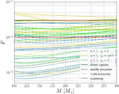
Figure 11: Optimized mismatches for equal mass nonspinning systems (blue), $q=\{2,3\}$ nonspinning (green), and spinning equal mass (yellow). For the $q=1$ nonspinning case we consider only the configurations with $E\leq 1.016\,M$. Scatterings are highlighted with dashed lines, double encounters with dash-dotted lines, direct merger with solid lines. The only triple-encounter of our dataset is denoted with a (blue) dotted line. The two red horizontal lines mark the $1\%$ and $3\%$ thresholds. The corresponding values for the reference mass $M=200M_{\odot}$ are reported in Table 2.

The scattering configurations have mismatches that are at the $10^{-3}$ level, even before the initial data optimization; the latter procedure only marginally improves the EOB/NR agreement. This result shows that TEOBResumS-Dalí is highly faithful in this energy and angular momentum regime, thus confirming the results discussed in Sec. III.3. On the contrary, the optimization is essential to lower the mismatches for configurations with multiple encounters. In particular, for the equal mass nonspinning cases with two encounters we have $\bar{F}_{\rm opt}\sim 1\%$. The triple encounter has instead an optimized mismatch that is below the $5\cdot 10^{-3}$ level. Improved initial data are also useful to lower the mismatches for some direct captures (solid lines). Interestingly, the optimization has a marginal effect on the direct captures with lowest angular momenta for each energy. This is probably a consequence of the fact that the ringdown part dominates these signals, while the ringdown model employed in TEOBResumS-Dalí is calibrated only on quasi-circular data. On the other hand, the optimization strongly improves $\bar{F}$ for direct captures with a quasi-circular whirl before the plunge. This occurs, for example, for the equal mass cases with $(\hat{E}_{0},p_{\varphi}^{0})\simeq(1.016,4.012)$, where the mismatch drop from $31.4\%$ to $0.5\%$ after optimization. The equal mass nonspinning configuration with lowest energy and angular momentum, $(\hat{E}_{0},p_{\varphi}^{0})\simeq(1.001,3.800)$, is the only direct capture without quasi-circular whirl whose mismatch is strongly improved by the optimization procedure (from $4.36\%$ to $0.27\%$). The mismatches for the equal mass nonspinning configurations are typically around or below the $1\%$ threshold after optimization. The two cases with higher final mismatches, that are direct captures with low angular momentum, are still within the $3\%$ threshold.

Generally, the nonspinning unequal mass configurations have higher mismatches than the previous case, but they are still within, or at most around, the $3\%$ threshold. On the other hand, for the spinning binaries we have three cases above the $3\%$ threshold, which however still remain below $5\%$.

We mention, in passing, that the $(q,\chi_{1},\chi_{2})=(1,0,0)$ cases with higher energies ($\hat{E}_{0}\geq 1.030$) require an optimization in a larger region, as can be imagined by looking at the results of Secs. III.2 and III.3. In these higher energy cases, the mismatches for the scattering configurations are typically below the $2\%$, while the merger configurations have $\bar{F}_{\rm opt}\sim 7-8\%$. The higher mismatches, together with the fact that the optimization has to be performed on a larger region, are a direct consequence of the lower reliability of TEOBResumS-Dalí in this energy regime.

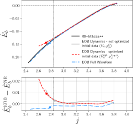
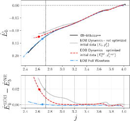
Figure 12: Energetic curves $\hat{E}_{b}(j)$ for the equal mass nonspinning dynamical capture, double encounter, and triple encounter with $\hat{E}_{0}=1.001$. The NR curves (black) are computed considering all the multipoles up to $\ell=5$, while the analytical gray and dashed red curves are obtained from the EOB dynamics, respectively before and after the initial data optimization discussed in Sec. III.4. We also show the energetics computed from the EOB waveform (dash-dotted blue), see text for details and interpretation. The EOB/NR differences are reported in the bottom panels. The NR merger time is marked with a dashed vertical line, while the estimated EOB merger times are highlighted with markers.

We conclude this section with a remark on the mass range shown in Fig. 11. The reason behind the choice $M\in[100,300]M_{\odot}$ is twofolds. On the one hand, the only significant event in the O3 LVK catalog Abbott et al. (2024, 2023) that can be interpreted as a dynamical capture is GW190521 Abbott et al. (2020); Gamba et al. (2023), which has a total source-frame mass of approximately $150M_{\odot}$. This is also the only significant intermediate mass BBHs observed so far Abbott et al. (2022). Secondly, taking into account lower masses would mean to only consider the low-frequency (in geometrized units) part of the waveform, i.e. the portion associated to the precursor. However, since we are integrating the numerical $\psi_{4}^{22}$ with a fixed-frequency method that removes the low-frequency part of the signal (see also discussion in Sec. II.3.1), the precursor of the numerical waveform is not reliable. Consequentely, the EOB/NR mismatches for initially unbound configurations can reach, and even overcome, the $10\%$ level in the low masses regime if FFI waveforms are employed. However, this is only an artefact of our numerical integration, and it is not related to the accuracy of the EOB model itself, that, thanks to the inclusion of the generic Newtonian prefactor Chiaramello and Nagar (2020), is indeed able to correctly reproduce the low-frequency part of the waveform.

The latter statement can be confirmed by considering a dynamical capture and computing $h_{22}$ with a TDI rather than an FFI. Time-domain methods, when practicable, are indeed able to reproduce the precursor of the numerical waveform. In general, the precursor is generated before the strong gravitational interaction of the two black holes, and therefore we expect to have the same precursor for all the configurations with same initial energy. We thus proceed by considering the nonspinning equal mass case with ($\hat{E}_{0},p_{\varphi}^{0})\simeq(1.011,3.950)$. We compute the numerical waveform with a time-domain integration, and then we calculate the EOB/NR mismatch. We find $\bar{F}_{\rm opt}\sim 2.5\%$ for $M\in[50,300]M_{\odot}$, and lower mismatches for lower masses. In particular, we find $\bar{F}_{\rm opt}=0.7\%$ for $10\,M_{\odot}$ .

III.5 EOB/NR energetics

While we have already presented some numerical energetic curves in Sec. II (and in particular in Figs. 2, 4 and 5), in this section we discuss the comparisons with the energetics obtained from TEOBResumS-Dalí. This test is indeed a well-established gauge-invariant diagnostic to the study the accuracy of the EOB dynamics Nagar et al. (2016); Damour et al. (2012). We recall that the numerical curves are obtained by subtracting from the initial values $(E_{0},p_{\varphi}^{0})$ the integrated energy and angular momentum fluxes, which we compute using all the multipoles up to $\ell=5$. The EOB counterparts are evaluated along the EOB dynamics, using in particular the time evolution of the Hamiltonian $H_{\rm EOB}$ and the canonical angular momentum $p_{\varphi}$ found by solving the equations of motion. We report in Fig. 12 the results for the series of simulations with the lowest initial energy considered in this work ($\hat{E}_{0}=1.001$). We select this series because it has a diverse range of coalescing phenomenologies: direct capture, double encounter, and triple encounter. For the proper EOB energetics computed from the dynamics, we report two different cases: i) the ones computed from the not-optimized NR initial data $(E_{0},p_{\varphi}^{0})$ (gray), ii) the curves obtained considering the initial data that optimize the mismatches as discussed in Sec. III.4 (dashed red); the enhanced initial data are also reported in Table 2. While the effect of the optimization is marginal (but not completely negligible) for the direct capture and the double counter, the improved initial data for the triple encounter provide a much more accurate curve. However, the optimization is also useful to improve the EOB/NR agreement for other direct captures and double encounters considered in this work. In general, we observe that the agreement between analytical and numerical results decreases towards the merger. While in the NR cases the merger time is identified by the last peak of the (2,2) amplitude (see also Appendix C), we recall that for the EOB case we estimate it from the peak of the pure orbital frequency computed without spin-orbit coupling as $t_{\rm mrg}^{\rm EOB}=t^{\rm peak}_{\Omega_{\rm orb}}-3$ Nagar et al. (2020). In particular, the EOB energetics obtained from the dynamics systematically end at higher energies and smaller angular momenta with respect to the NR case. It should be however considered that these analytical energetics are computed from the dynamics, and therefore they do not contain any contribution from the quasi-circular ringdown model of TEOBResumS-Dalí. In other words, the most significant comparison between the analytical and numerical results is for the pre-merger portion of the evolution, where the agreement is indeed better.

To confirm the latter statement, we also compute the integrated analytical fluxes from the complete optimized EOB waveform, and subtract them to the initial data. The corresponding energetics are shown with dash-dotted blue lines in Fig. 12. Note that these EOB curves are less meaningful than the ones previously discussed, since the energetics are mainly a diagnostic for the dynamics. However, they are still useful to highlight that the inclusion of a ringdown model in the EOB waveform makes the analytical results closer to the numerical curves also after the merger. The small discrepancies between the energetics computed from the EOB dynamics and the EOB waveform are mainly linked to the fact that each multipole of the waveform includes a noncircular Newtonian correction Chiaramello and Nagar (2020); Albanesi et al. (2021) (see also discussion in Sec. IV.3), while the angular radiation reaction ${\cal F}_{\varphi}$ only include the (2,2) Newtonian noncircular correction. Moreover, when computing the EOB fluxes, we sum up to $\ell=5$ for consistency with the NR curves, while the EOB dynamics incorporates multipoles up to $\ell=8$. However, we checked that these additional modes are highly subdominant during the inspiral, and are not a primary source of discrepancy. Note that in the EOB/NR difference computed considering the energetics from the EOB waveform, there is a small jump near the EOB merger time. This discontinuity arises because the NQC corrections were not included in the computation of the EOB waveform.

We conclude this discussion by recalling that the TEOBResumS-Dalí dynamics is only numerically informed through the $a_{6}$ and $c_{3}$ coefficients, that are tuned on quasi-circular NR simulations. As already mentioned when analyzing other diagnostics, the inclusion of non-circularized simulations in this procedure, together with more non-circular analytical information, would probably further improve the model, and thus the comparisons of the energetics.

IV Test-mass limit

  

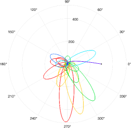
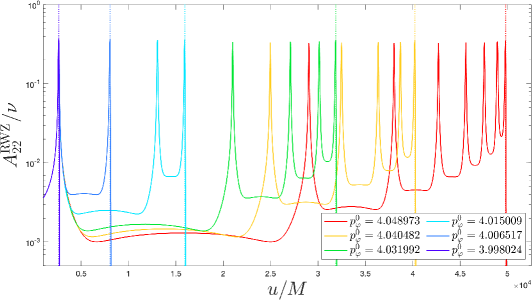
Figure 13: Left panel: trajectories for test-mass dynamical captures with $\nu=10^{-2}$, $r_{0}=300$, and $\hat{E}_{0}=1.000001$. The black dot marks the initial position, that is the same for all configurations. Right panel: corresponding (2,2) Zerilli $\nu$-rescaled amplitudes computed with the time-domain code RWZHyp; vertical logarithmic scale. The initial angular momenta are reported in the legend. The vertical dotted lines mark the amplitude maxima.

While extreme mass-ratio inspirals (EMRIs) might be relevant for future space-based detectors, such as LISA Babak et al. (2017); Berry et al. (2019), the test-particle limit is also an useful controlled laboratory to test and validate analytical prescriptions for binaries with generic mass ratio Nagar et al. (2007); Damour and Nagar (2007); Bernuzzi et al. (2011b); Albanesi et al. (2021); Placidi et al. (2022); Albanesi et al. (2023). In particular, the test-mass limit is naturally included in the EOB approach, since the effective EOB metric is a $\nu$-deformation of the Schwarzschild metric (or the Kerr one, if spinning black holes are considered). For these reasons, we now shift our focus to test particles captured by Schwarzschild black holes. Corresponding waveforms at linear order in the mass ratio can be derived as solutions of the RWZ equations with a test particle source term Regge and Wheeler (1957); Zerilli (1970); Nagar and Rezzolla (2005); Martel and Poisson (2005). These equations are solved numerically with the time-domain code RWZHyp Bernuzzi and Nagar (2010); Bernuzzi et al. (2011a, 2012). We then compare the numerical results with the corresponding fully analytical EOB waveforms, adopting different prescriptions for the non-circular corrections.

IV.1 Test-particle dynamics

Time-like geodesics in Schwarzschild spacetime can be conveniently parametrized by the Schwarzschild coordinate time, so that the test-particle Hamiltonian depends only on spatial coordinate and momenta. More specifically, the $\mu$-rescaled Hamiltonian reads

$${\hat{H}_{\rm Schw}}=\sqrt{A(r)\left(1+\frac{p_{\varphi}^{2}}{r^{2}}\right)+p_{r_{*}}^{2}},$$ (13)

where $p_{r_{*}}$ is the conjugate momentum of the tortoise coordinate $r_{*}$, defined as $p_{r_{*}}^{2}=A/B\,p_{r}^{2}$. The Schwarzschild metric potentials $A$ and $B$ are defined as $A=1-2/r$ and $B=A^{-1}$. It is useful to explicitly keep $B$ in the formal definition of $p_{r_{*}}$, so that it remains valid in the Kerr and EOB cases with opportune generalizations of these two metric potentials Damour and Nagar (2014). Dissipative effects linked to the GW emission can be included in the dynamics by adding a radiation reaction force ${\cal F}$. The equations of motion thus read

$$\dot{r}= \frac{A}{{\hat{H}_{\rm Schw}}}p_{r_{*}},$$ (14)

$$\dot{\varphi}= \frac{A}{{\hat{H}_{\rm Schw}}}\frac{p_{\varphi}}{r^{2}},$$ (15)

$$\dot{p}_{r_{*}}= A\hat{{\cal F}}_{r}-\frac{A}{r^{2}{\hat{H}_{\rm Schw}}}\left[p_{\varphi}^{2}\left(\frac{3}{r^{2}}-\frac{1}{r}\right)+1\right],$$ (16)

$$\dot{p}_{\varphi}= \hat{{\cal F}}_{\varphi},$$ (17)

where $\hat{{\cal F}}_{r,\varphi}\equiv{\cal F}_{r,\varphi}/\nu$ are the radial and angular components of the radiation reaction force. For this term we use the resummed PN expressions discussed in Ref. Chiaramello and Nagar (2020) and extensively tested for bound dynamics in Ref. Albanesi et al. (2021). We consider systems with $\nu=10^{-2}$. This choice only affects the relevance of the radiation reactions during the inspiral, since no $\nu$-corrections are included in the conservative dynamics, that is fully described by Eq. (13). However, for the description of astrophysical EMRIs, one should consider an EOB Hamiltonian informed with gravitational self-force (GSF) results, as detailed in Refs. Nagar and Albanesi (2022). Fluxes with higher-order PN corrections has been also proven to be essential to consistently reproduce GSF calculations Albertini et al. (2022a, b, 2024). However, as mentioned earlier, in this analysis we are interested in using the waveforms generated by a test-mass dynamical capture to assess the analytical EOB prescription for the waveform, and also to gain insights into properties of the numerical waveform. For these reasons, the prescription of the radiation reaction discussed in Refs. Chiaramello and Nagar (2020); Albanesi et al. (2021) is more than sufficient for our goals.

The trajectories of six dynamical captures with initial separation $r_{0}=300$, initial energy $\hat{E}_{0}=1.000001$, and different initial angular momenta are shown in the left panel of Fig. 13. The angular momenta, whose values are reported in the legend of the right panel, are chosen by requiring to have multiple encounters in a reasonable time window. Since for high-mass ratios the relevance of the radiation reaction is inhibited, we chose an initial energy just above the parabolic limit, in order to obtain captures with multiple encounters. This result also points out that the initially unbound portion of the parameter space for large mass ratio binaries is largely dominated by scattering and direct captures Nagar et al. (2021a). Depending on formation scenarios, comparable masses BBHs might be more likely to be sources of dynamical captures with multiple close encounters.

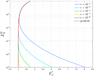
Figure 14: Impact of the radiation reaction on the the critical initial angular momentum $p_{\varphi}^{*}$ at which the scattering-capture transition occurs in the test-particle limit. On the $y$-axis we show the initial (not $\nu$-reduced) binding energy $E_{b}^{0}\equiv\hat{E}_{0}-1$ in logarithmic scale. Solid lines are obtained by considering EOB evolutions with different symmetric mass ratios, whose effects are solely included in the dissipative sector. In all the cases, we start the evolution from $r_{0}=300$. The black dashed line marks the geodesic case ($\nu=0$), computed fully analytically from Eq. (18).

The relevance of the radiation reaction is also visualized in Fig. 14, where we show the critical initial angular momentum $p_{\varphi}^{*}$ at which the scattering-capture transition occurs for different mass ratios and energies. While for $\nu\neq 0$ we have a dissipative contribution to the dynamics and we need to use a numerical ODE solver for the Hamilton’s equations, for the geodesic case the critical angular momentum can by computed as Damour and Rettegno (2023)

$$p_{\varphi}^{*,{\rm Schw}}=\sqrt{\frac{1}{u_{0}^{2}}\left(\frac{\hat{E}^{2}}{1-2u_{0}}-1\right)},$$ (18)

where

$$u_{0}=\frac{4-3\hat{E}^{2}+\hat{E}\sqrt{9\hat{E}^{2}-8}}{8}.$$ (19)

As can be appreciated from Fig. 14, the region of the parameter space in which dynamical captures with multiple encounters are allowed strongly shrinks with the mass ratio, and, for the energies considered, practically vanishes for $\nu=10^{-6}$. Finally, while the geodesic case leads to a logarithmic divergence Damour and Rettegno (2023) in the scattering angle at $p^{*}_{\varphi}(\hat{E})$, the presence of a radiation reaction limits these angles to finite values.

IV.2 Numerical solution of RWZ equations

Given the test-particle dynamics discussed in the previous section, we can compute the corresponding waveform at linear order in perturbation theory by solving the inhomogeneous RWZ equations with test-particle source term Regge and Wheeler (1957); Zerilli (1970); Nagar and Rezzolla (2005); Martel and Poisson (2005),

$$\partial_{t}^{2}\Psi_{\ell m}^{(o/e)}-\partial^{2}_{r_{*}}\Psi_{\ell m}^{(o/e)}+V_{\ell}^{(o/e)}\Psi_{\ell m}^{(o/e)}=S_{\ell m}^{(o/e)},$$ (20)

where the master function $\Psi_{\ell m}^{(o/e)}$ is linked to the waveform multipoles by a simple normalization $\Psi_{\ell m}^{(o/e)}=h_{\ell m}/\sqrt{(\ell+2)(\ell+1)\ell(\ell-1)}$. We solve these equations with the time-domain code RWZHyp Bernuzzi and Nagar (2010); Bernuzzi et al. (2011a, 2012), where the Dirac $\delta$ in the source term $S_{\ell m}^{(o/e)}$ is approximated by a narrow Gaussian. Since the motion of the particles can extend to large separations ($r\sim 500$), a large computational domain is needed. We thus use as time and radial coordinates $(\tau,\rho)\in\mathbb{R}\times[R_{*}^{-},S^{+}]_{R_{*}^{+}}=\mathbb{R}\times[-100,700]_{600}$, that coincide with the Schwarzschild time and tortoise radial coordinates in the compact region $[R_{*}^{-},R_{*}^{+})$, where the motion of the particle is confined. An hyperboloidal layer Zenginoğlu (2011); Bernuzzi et al. (2011a) is then matched to these coordinates at $\rho=r_{*}=R_{*}^{+}$. The compactification variable $\rho(r_{*})$ maps $[R_{*}^{+},\infty)$ in $[R_{*}^{+},S]$. The time coordinate $\tau$ is determined requiring that the time Killing vector is the same in the two coordinate systems, and that the outgoing light-rays are left invariant. Within these choices, the surface $\rho=S$ corresponds to future null infinity, $S^{+}$, where the waveform is extracted, avoiding in this way errors linked to finite-distance extraction. The grid is uniform with radial step $\Delta\rho=0.02$, and the time evolution is performed with a 4th-order Runge-Kutta scheme.

The amplitudes of the (2,2) Zerilli waveforms that corresponds to the dynamics discussed in the previous section are shown in the right panel of Fig. 13. An interesting feature is that the waveform generated near the apastron is non-vanishing, and its relevance increase as the particle loses energy; this is particularly evident for the configurations with many encounters before merger. Since this portion of the waveform corresponds to a low orbital (and thus waveform) frequency, this feature is lost when integrating with a frequency cut-off, as in the FFI methods that we use to obtain $h_{\ell m}$ from $\psi_{4}^{\ell m}$ in the comparable mass case. In Appendix B, we use these test-mass data to gain insight on the numerical integration of $\psi_{4}^{\ell m}$ performed in the comparable mass case.

IV.3 Noncircular EOB waveforms in the test-mass limit

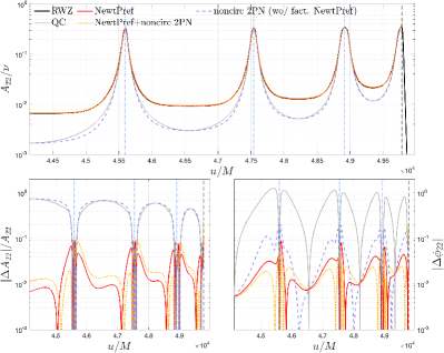
Figure 15: Zerilli (black) and EOB (2,2) waveforms evaluated along the last part of the test-particle dynamics with $p_{\varphi}^{0}=4.04897$ (red lines in Fig. 13). Periastra are marked with dash-dotted vertical lines, while the dashed vertical line marks the peak of $A_{22}^{\rm RWZ}$. We consider different EOB noncircular corrections: i) none (solid gray), ii) generic Newtonian prefactor (solid red), iii) 2PN with generic NP factorization (dotted orange), iv) 2PN without generic NP factorization (dashed blue). In the bottom panels we report the phase and relative amplitude differences for each analytical prescription.

Capturing the correct waveform behavior in highly eccentric configurations is a delicate matter, and not all the prescriptions with noncircular information at the same PN order provide comparable results. We will thus use the Zerilli waveforms discussed in the previous section to test the analytical EOB prescriptions for the inspiral waveform and establish which one it the most accurate.

We start by recalling the analytical structure of the EOB inspiral waveform. Each multipole is factorized as Damour et al. (2009); Placidi et al. (2022)

$$h_{\ell m}=h_{\ell m}^{(N,\epsilon)_{\rm c}}\hat{h}_{\ell m}^{(N,\epsilon)_{\rm nc}}\hat{h}_{\ell m}^{(\epsilon)_{\rm c}}\hat{h}_{\ell m}^{(\epsilon)_{\rm nc}},$$ (21)

where $\epsilon$ marks the parity of the modes; we have $\epsilon=0$ for even modes ($\ell+m$ even), 1 otherwise. The factors in Eq. (21) are briefly discussed in the following.

• $h_{\ell m}^{(N,\epsilon)_{\rm c}}$ is the Newtonian circular term that, aside from a normalization, it is given by $\propto\left(r\Omega\right)^{\ell+\epsilon}e^{-im\varphi}$.

• $\hat{h}_{\ell m}^{(N,\epsilon)_{\rm nc}}$ is the noncircular Newtonian correction, written in terms of explicit time-derivatives of the radius and frequency Chiaramello and Nagar (2020). For the (2,2) mode, this correction reads

  $$\hat{h}_{22}^{(N,0)_{\rm nc}}=1-\frac{\ddot{r}}{2r\Omega^{2}}-\frac{\dot{r}^{2}}{2r^{2}\Omega^{2}}+\frac{2\mathrm{i}\dot{r}}{r\Omega}+\frac{\mathrm{i}\dot{\Omega}}{2\Omega^{2}}.$$ (22)

  This contribution, together with $h_{\ell m}^{(N,\epsilon)_{\rm c}}$, constitutes the generic Newtonian prefactor.

• $\hat{h}_{\ell m}^{(\epsilon)_{\rm c}}$ is the PN circular correction, that is further factorized in effective source term, tail contribution, and residual phase/amplitude series Damour et al. (2009). The resummation of these series is a crucial aspect of the model, especially for the amplitude corrections known as $\rho_{\ell m}$ Messina et al. (2018); Nagar et al. (2019).

• $\hat{h}_{\ell m}^{(\epsilon)_{\rm nc}}$ is the noncircular PN correction Khalil et al. (2021); Placidi et al. (2022); Albanesi et al. (2022b); Placidi et al. (2023), where the instantaneous part is written as discussed in Ref. Albanesi et al. (2022b), and the eccentric tail is taken from Ref. Placidi et al. (2022); for the latter, we consider the expression written in terms of $\left(r,p_{r_{*}},\dot{p}_{r_{*}}\right)$. We remark that the eccentric tail is obtained from a low-eccentricity expansion, and that we consider the expressions up to 2PN. This factor is not included yet in TEOBResumS-Dalí, but has been tested in previous works Placidi et al. (2022); Albanesi et al. (2022b).

Due to the finite PN accuracy, the choice of the factorization and subsequent resummation is a crucial in order to obtain accurate EOB waveforms. In particular, it has been shown in previous works that the factorization of the noncircular Newtonian correction $\hat{h}_{\ell m}^{(N,\epsilon)_{\rm nc}}$ strongly improves the analytical/numerical agreement for noncircular planar dynamics Placidi et al. (2022); Albanesi et al. (2022a, b). We thus perform a similar test also in the dynamical capture scenario considered in this work.

Among the ones shown in Fig. 13, we analyze in detail the configuration with highest number of close encounters. Then, in Fig. 15, we compare the numerical waveform with different analytical prescriptions. Each analytical waveform is computed up to the amplitude peak of the Zerilli waveform. We do not complete the analytical waveforms with a ringdown model, nor we apply NQC corrections. The first analytical prescription that we consider is the quasi-circular one (solid gray), that, not surprisingly, is not able to correctly reproduce the amplitude and the phase of the Zerilli waveform. Even the solely inclusion of the Newtonian noncircular correction produces a waveform that is far more accurate (solid red), especially at apastron, when the particle reaches the highest orbital separation from the Schwarzschild black hole. The strong improvement of the analytical waveform near the apastron was also noted in Ref. Albanesi et al. (2022b) for eccentric configurations (see Fig. 2 therein). The addition of 2PN noncircular terms to the Newtonian-factorized prescription provides a small correction to the waveform (dotted orange), marginally improving the phase. However, the inclusion of 2PN corrections without factorizing the generic Newtonian prefactor yields a waveform (dashed light-blue) whose amplitude is not reliable, especially at apastron. Only the phase is improved with respect to the quasi-circular waveform, but still performs worse than the prescriptions with the factorization of the generic Newtonian prefactor. A similar result was found in Ref. Placidi et al. (2022), where fully PN-expanded prescriptions, such as the one proposed in Ref. Khalil et al. (2021), and waveforms with the generic Newtonian prefactor factorized, such as the one considered in TEOBResumS-Dalí, were tested against numerical data. While the phase was accurate for the whole inspiral for both typologies, the amplitude of the fully PN-expanded waveform performed poorly at apastron, especially for highly-eccentric binaries (see Fig. 15 and 18 of Ref. Placidi et al. (2022)). The findings depicted in Fig. 15 further support these observations, indicating the necessity to refrain from PN-expanding the time-derivatives, at least at Newtonian level, to accurately describe the amplitude at apastron. In this way, these derivatives are evaluated using the complete equations of motion rather than the PN-expanded ones. When computing the waveform from the dynamics, these derivatives can be easily obtained by numerical differentiation. However, when higher-order time derivatives are included in the radiation reaction, an iterative procedure has to be used in order to solve the Hamilton’s equations with a standard ODE integrator Damour et al. (2013); Chiaramello and Nagar (2020).

V Conclusions

Several aspects of this work involved investigating initially unbound comparable mass two-black-hole systems, which can result in either scatterings or dynamical captures, depending on the impact of the back-reaction of the GW emission. As a part of this study, we have performed NR simulations for 84 physical configurations, including nonspinning systems up to mass ratio $q=3$ and equal mass cases, both with and without spin. Largely guided by the predictions of the state-of-the-art EOB model TEOBResumS-Dalí Nagar et al. (2023, 2024), we have chosen NR initial data with the goal of reproducing a large set of phenomenologies. Varying the initial energy and angular momentum, we have then performed the time evolution of different physical systems with the code GR-Athena++ Daszuta et al. (2021); Cook et al. (2023). Afterwards, we have discussed the post-processing applied to the output of the NR code explaining, in particular, the procedures followed to compute strains, scattering angles, and energetics. Different physical configurations have been further examinated in Sec. II.4, focusing on the phenomenology of waveforms and dynamics; in the case of coalescing systems, we also studied the properties of the remnants. Of the different $(q,\chi_{1},\chi_{2})$-configurations considered in this work, the equal mass nonspinning case is the one that has been studied in greater detail. Regressions of the scattering-capture transition in the latter case have been also presented in Sec. II.4.1, and subsequently compared with the recent results of Ref. Kankani and McWilliams (2024), finding consistency between the two estimates.

Dalí, the avatar of TEOBResumS considered in this work, has been also compared with the aforementioned numerical results in Sec. III. After having discussed the prediction of the analytical model across the parameter space, we have examined its agreement with the NR simulations. Lending focus on the scattering-capture transition, we found a remarkable EOB/NR agreement for initial energies up to $E_{0}\sim 1.02\,M$; the EOB/NR agreement also enconpass scattering angles, as discussed in Sec. III.3. Inevitably, the EOB model loses reliability for higher energies, especially near the transition region, since the EOB Hamiltonian and the radiation reaction are PN-approximate, and thus not reliable for high velocities; however, the analytical/numerical agreement is progressively restored for large angular momenta, even at the highest energy considered in this work ($E_{0}\sim 1.05\,M$).

We then shifted our attention to the mismatches between EOB and NR (2,2) waveforms, showing that the unfaithfulness computed with the LIGO noise is typically below the $1\%$ for the configurations with $E_{0}\lesssim 1.02\,M$, with a few cases that reach the $3\%$. Improving the ringdown model adopted in TEOBResumS-Dalí is necessary to further enhance the agreement in the direct capture scenario. Note that the current post-merger model implemented in our EOB model is indeed informed only on quasi-circular data, but an extension to generic planar orbits could be achieved following the path traced in Ref. Carullo et al. (2024). Scatterings show the lowest mismatches among the configurations examined, while the unfaithfulness for the multiple encounters typically lays in between these unbound configurations and direct captures.

In recent years PM computations for the dynamics of two-body systems have been conducted using a variety of methods, some of which adapted from the field of particle physics, e.g. Guevara et al. (2019); Bern et al. (2019, 2021, 2022); Manohar et al. (2022); Saketh et al. (2022); Di Vecchia et al. (2021, 2022); Mogull et al. (2021); Riva and Vernizzi (2021); Jakobsen et al. (2021, 2022); Dlapa et al. (2022a, b, 2023, 2024); Bini et al. (2021); Bini and Damour (2022); Bini et al. (2023). The inclusion of these recent PM results in the EOB dynamics is not a trivial task Bini and Damour (2018); Antonelli et al. (2019); Buonanno et al. (2024), and even the PM predictions for scattering angles need a proper EOB-inspired resummation to provide results in agreement with NR simulations, especially for low impact parameters Damour and Rettegno (2023); Rettegno et al. (2023). However, the inclusion of PM results in the EOB dynamics should be further studied to improve EOB models in the high velocity regime, where PN results naturally lose their reliability.

Finally, the test-mass limit studied in Sec. IV reaffirms its utility as a controlled laboratory setting for gaining deeper insights into properties that are also applicable to comparable mass binaries. In particular, the numerical waveforms found by solving the Zerilli equation have been used to: i) corroborate the higher accuracy of the analytical noncircular corrections proposed in Refs. Chiaramello and Nagar (2020); Placidi et al. (2022); Albanesi et al. (2022b) compared to noncircular corrections fully expanded with the PN equations of motion, ii) gain insights on the numerical integration procedure carried out in the NR case.

On the numerical side, future explorations will involve different aspects. First of all, producing more accurate numerical waveforms for scattering and captures is of primary interest, since they are the benchmark to validate and calibrate semi-analytical models. While the standard extraction of the Weyl scalar at finite distance can still be used to obtain the strain by numerical integration, CCE Bishop et al. (1998); Babiuc et al. (2011) or metric perturbations extraction Abrahams and Price (1996); Pazos et al. (2007); Bishop and Rezzolla (2016) would probably provide more reliable results. Secondly, while we started to explore also unequal mass configurations and spin effects, a more refined exploration is needed in order to extend the calibration, and thus the reliability, of analytical models.

Ultimately, the outcomes of this research underline the synergies between numerical and analytical methods. While numerical simulations are crucial for validating and informing semi-analytical models, predictions from robust analytical techniques can offer a preliminary exploration of the parameter space and indicate the regions where NR simulations should be focused.

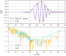
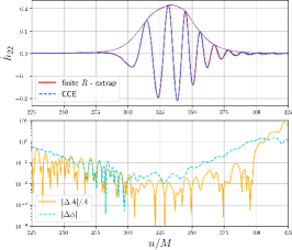
Figure 16: Comparisons between extrapolated finite-distance waveforms (solid red) and CCE waveforms (dashed blue) for the equal mass nonspinning configuration with $(\hat{E}_{0},p_{\varphi}^{0})\simeq(1.011,3.950)$. We show, from left to right, $\psi_{4}^{22}$, $\dot{h}_{22}$, and $h_{22}$. In the CCE case, we extract the News at infinity and we obtain the Weyl scalar and the strain by numerical derivation and integration, respectively. Finite-distance waveforms are obtained in post-processing from $\psi_{4}$ as detailed in Sec. II.3.1. In the bottom panels we show the phase differences in radians (dashed cyan) and the relative amplitude differences (solid orange).

Appendix A CCE waveforms

As mentioned in Sec. II.3.1, we also computed CCE waveforms using the public code PITTNull Bishop et al. (1998); Babiuc et al. (2011) for some configurations. The metric fields are expanded Babiuc et al. (2011) and the coefficients are stored during the GR-Athena++ evolution at every $10$th time step of evolution and for eight different radial intervals, ranging from $[76,84]\,M$ to $[296,304]\,M$ (see midpoints below). These expansion coefficients are used to construct the initial data in the PITTNull code. Additionally, we set the radius of the initial data world tube at the middle of each extraction interval, so that we have $R_{w}=\{80,90,100,120,140,160,200,300\}\,M$.

Unfortunately, the expansion coefficients include numerical noises Babiuc et al. (2011); leaving these numerical noises untreated and carrying them into the initial data of the PITTNull code, introduce even larger noises in the final solution of nonlinear characteristic equations Babiuc et al. (2011). As such, we remove the high-frequency noises using the built-it filter fftwfilter with a max frequency of $\omega_{\rm max}=1.5\,M^{-1}$.

CCE data for a significant physical configuration are reported in Fig. 16 (dashed blue). More precisely, we consider the News given in output by PITTNull for $R_{w}=200\,M$. The Weyl scalar is then obtained by numerical differentiation with a 4th-order centered stencil scheme; we checked that this result is equivalent to the Weyl scalar given directly by PITTNull. The CCE strain is instead obtained by applying an FFI to the News with cut-off frequency $f_{0}=0.007\,M^{-1}$. Despite the need of just one integration step, time-domain methods seem to not yield reliable strains; this issue may be linked to high-frequency noise still present in our CCE data. We select a large radius because the initial portion of the News for small world tubes exhibits an unphysical bump, which tends to diminish only for larger radii. This is likely associated with the proximity to the punctures at the beginning of the simulation. Since the CCE waveform with $R_{w}=300\,M$ is visibly affected by numerical dissipation, we consider the previous radius, i.e., $R_{w}=200\,M$.

In Fig. 16 we also report the extrapolated finite-distance waveform, computed by integrating the extrapolated Weyl scalar, that is obtained from Eq. (3) using $\psi_{4}^{22}$ extracted at $R=100\,M$. The integration steps are performed in a similar manner to the CCE case, employing an FFI with $f_{0}=0.007\,M^{-1}$, which is also the standard procedure used throughout this paper for equal mass binaries, as detailed in Sec. II.3.1.

The relative amplitude differences (solid orange) and the phase differences (dashed light-blue) between the two different methods are reported in the bottom panels of Fig. 16. As can be seen, these difference are quite large for the precursor and the ringdown. This is however expected, since in these cases the signal is weaker, and thus more difficult to resolve and contaminated by numerical noise. We thus mainly focus our discussion on the GWs generated by the close encounter and the subsequent merger.

The comparison reveals that the amplitude difference for $\psi_{4}^{22}$ is not completely negligible, even in the aforementioned time window, where it oscillates between $\sim 0.2\%$ and $\sim 4\%$. The phase difference reaches at most the 0.05 radians before merger, but rapidly increases afterwards. Similar discrepancies are observed for $\dot{h}_{22}$. The differences for the strain are instead higher, reaching $|\Delta A|/A\sim 10\%$ and $|\Delta\phi|\sim 0.1$ radians even during the close encounter/merger. The amplitudes of the strain reported in the right upper panel show a priori unexpected oscillations, both in the CCE and extrapolated finite-distance waveforms. This is likely to be an artefact of the FFI, since these oscillations increase for lower cut-off, and decrease for higher ones.

The test performed in this appendix indicates that obtaining accurate CCE waveforms for dynamical capture is not straightforward and poses several challenges. However, the presence of less integration steps with respect to the extrapolation of finite distance waveforms, together with the direct computation at future null infinity, lead us to think that, with improved CCE data, it should be possible to obtain more accurate results. CCE waveforms should be revisited in future works, considering for example improved high-frequency filters. We postpone a more thoughtful analysis to the future.

Appendix B Integration tests in the extreme mass-ratio limit

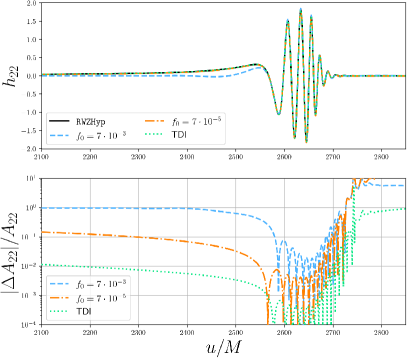
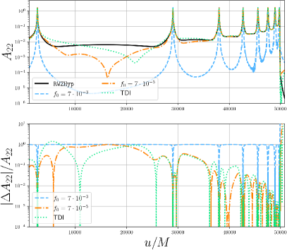
Figure 17: Left panels: Real part of the (2,2) Zerilli waveform obtained by solving numerically Eq. (20) with RWZHyp along the a dynamics with $\nu=10^{-2}$, $r_{0}=300$, $\hat{E}_{0}=1.000001$, and $p_{\varphi}^{0}=3.988024$. This waveform (black) is compared with different integration tests, obtained by double-integrating the second time derivative of the solution. We consider FFI with two different frequency cut-offs, $f_{0}=7\cdot 10^{-3}$ (dashed blue) and $f_{0}=7\cdot 10^{-5}$ (dot-dashed orange), and a time-domain integration where the numerical drift is removed by subtracting a fitted constant at each integration step (dotted green). The relative amplitude difference with the original Zerilli waveform are shown in the bottom panel with the same color scheme. Right panels: similar analysis for the configuration with $p_{\varphi}^{0}=4.048973$; in the upper panel we show the amplitude in logarithmic scale rather than the real part.

Waveforms generated by test-particle dynamics can be obtained by numerically integrating the RWZ equations (20). To accomplish this task, we use the time-domain code RWZHyp, that extracts the waveform at future null infinity. On the contrary, the NR code GR-Athena++ produces the Weyl scalar $\psi_{4}^{\ell m}=\ddot{h}_{\ell m}$ at finite distance (if no CCE is used), so that in order to obtain the strain at future null infinity we need three integration steps: one to extrapolate $\psi_{4}^{\ell m}$ using Eq. (3), and two additional steps to obtain $h_{\ell m}$. As argued in Sec. II.3, through this paper we have used an FFI with cut-off at $f_{0}=0.007\,M^{-1}$. This precise value is not strictly physically motivated, but cut-off at higher frequencies would remove a large portion of the signal, while too low cut-off frequencies would generate evident drifts in the NR waveform.

We can thus use the RWZ waveforms to test the TD and FD integrations. After having obtained $h_{22}$ by numerically solving the Zerili equation with RWZHyp, we compute $\psi_{4}^{22}$ by computing the second-time derivative with a 4th-order centered stencil scheme. The Weyl scalar is then integrated back with different methods. We start by considering, as a show-case example, the test-mass dynamical capture with lowest angular momentum, that is indeed a direct capture. We start by considering an FFI with cut-off frequency $f_{0}=0.007\,M^{-1}$, similarly to the NR case; the result is shown in the left panels of Fig. 17 with a dashed blue line. Comparing this waveform with the one obtained directly from RWZHyp (black line), it is immediately clear the precursor of the FFI waveform is not reliable. This fact is made even more explicit by the relative amplitude difference shown in the bottom panel. The FFI wave becomes more accurate for the merger-ringdown signal, but the discrepancies with the RWZHyp amplitude are still between the $1-8\%$. Since the test-mass waveforms produced by RWZHyp are not contaminated by noise as much as the full NR ones, we can consider a lower cut-off frequency. The result for $f_{0}=7\cdot 10^{-5}$ is shown with a dot-dashed orange line. This waveform is more reliable during the whole evolution with respect to the previous case, but especially for the low-frequency precursor. However, the amplitude of the precursor is still off by a $10\%$, while the error on the amplitude during the merger drops below the $1\%$. Smaller cut-off frequencies do not improve this result, and eventually lead to greater discrepancies. An even more accurate waveform can be obtained with a time-domain integration, where at each step we subtract an integration constant determined by a fit on the last portion of the post-merger waveform (after the quasi-normal-mode ringing). The latter result is shown with a dotted green line. The relative amplitude difference with the precursor of the RWZHyp waveform is at the $1\%$ level, and the difference drops below the $10^{-3}$ threshold during the merger/early ringdown. Similar results can be obtained also for the other test-mass configurations with more encounters, as shown by the case reported in the right panels of Fig. 17. Note, however, that for this very long signal, none of the integration methods is able to correctly reproduce the waveform at the first apastron passage. The accuracy of all the integration methods increases with the proximity to the merger.

This results show that, when applicable, time-domain methods should be preferred to FFI. However, in the NR case the former method works only for a few cases, typically for signals with a short duration, such as direct captures. Longer waveforms, like those generated by double encounters, require an FFI. While the test-mass results seem to suggest that the cut-off frequency used in the NR case is rather large, we recall that the FFI procedure adopted in this paper yields reliable remanent properties, that are computed from the energetics $\hat{E}_{b}(j)$, and thus from the waveform through Eqs. (5). This was explicitly checked in Sec. II.5, where the differences between remnant properties obtained with FFI and time-domain integrations were $(\Delta\hat{M},\,\Delta\hat{a}_{f})=(0.0015,\,0.0058)$ for the nonspinning equal mass configuration with $(\hat{E}_{0},\,p_{\varphi}^{0})\simeq(1.011,\,3.950)$. Similarly, for this configuration the EOB/NR mismatch was not significantly affected by the integration method in the mass range $M\in[100,300]M_{\odot}$, as discussed at the end of Sec. III.4.

Appendix C Merger time for generic orbits

For spin-aligned, equal mass, quasi-circular BBHs, the merger time $t_{\rm mrg}$ is typically defined as the global peak of the (2,2) amplitude. However, in highly eccentric binaries, the highest peak might not be the one associated with the merger of the two black holes. Indeed, it can happen that bursts generated by previous close encounters have higher peaks, as already noted in Ref. Carullo et al. (2024). For this reason, we propone to define the merger time $t_{\rm mrg}$ as the time that corresponds to the last peak of the (2,2) amplitude. To avoid considering local peaks associated to mode-mixing, rather than to the coalescence of the two black holes, we also require that the peak is above the threshold $\epsilon_{A}=0.2A^{\max}_{22}$, where $A^{\max}_{22}\equiv\max(A_{22})$ is the global maximum of the amplitude.

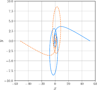
Figure 18: Left panel: tracks of the punctures for the nonspinning equal mass configuration with $(\hat{E}_{0},p_{\varphi}^{0})\simeq(1.016,4.180)$. Right panel: real part and amplitude of the corresponding (2,2) waveform (black and green, respectively). The dashed orange line marks the merger time, defined as the last $A_{22}$ peak, while the blue dotted line highlight the global maximum of the amplitude. The visible artefacts in the amplitudes are linked to integration and are also discussed in Appendix C.

We report in Fig. 18 an example that clarifies the necessity of this definition. We consider an equal mass nonspinning double encounter with initial energy $E_{0}\simeq 1.016\,M$ and angular momentum $p_{\varphi}^{0}\simeq 4.180$. The global maximum of the invariant amplitude occurs at $u\simeq 280\,M$, in correspondence of the first close encounter, where $A_{22}^{\rm max}\sim 0.57$. On the other hand, the last maximum occurs at $u\simeq 650\,M$, shortly before the beginning of the ringdown phase, where the amplitude only reaches $A_{22}^{\rm mrg}\sim 0.43$, so that the ratio with the global maximum is $A_{22}^{\rm mrg}/A_{22}^{\rm max}\sim 0.75$. Higher initial energies can even decrease this proportion; for the equal mass nonspinning configuration with $(E_{0},p_{\varphi}^{0})\simeq(1.051,4.755)$, we get $A_{22}^{\rm mrg}/A_{22}^{\rm max}\sim 0.52$. For higher energies than the ones considered in this work, the ratio might be even more unbalanced, but we recall that the width of the double encounter region of the parameter space shrinks for increasing energies, making these configurations less likely to occur (see, e.g., Fig. 8 and 9).

We also make a remark on the effects of the integration procedure. As can be clearly seen from the amplitude reported in Fig. 18, $A_{22}$ exibhits a double peak in correspondence of the first encounter. However, this is only an artefact linked to the cut-off frequency used in the FFI. Indeed, higher cut-offs yield only one peak, but also remove more physical frequencies from the signal. As a consequence, fluxes computed with greater cut-offs are underestimated. This further suggests that the post-processing of $\psi_{4}$ for dynamical captures and scattering is indeed a delicate matter, and alternative methods to extract the strain should be considered.

We conclude this discussion by emphasizing that in cases where higher modes significantly contribute to the strain, such as BBHs with higher mass ratios or precessing dynamics, it is more appropriate to consider the invariant amplitude $A_{\rm inv}$ instead of the (2,2) waveform amplitude. This quantity is defined as Schmidt et al. (2017)

$$A_{\rm inv}=\sqrt{\sum_{\ell m}|h_{\ell m}|^{2}},$$ (23)

where $h_{\ell m}$ are the multipoles of the waveform in the co-precessing frame. In this work we study spin-aligned systems, so that the difference between $A_{\rm inv}/\sqrt{2}$ and $A_{22}$ is in practice negligible, especially for the determination of the merger time. Nevertheless, the two quantities differ for precessing binaries or high mass ratios, so that $A_{\rm inv}$ is in general preferred.

Table 2: Optimized and not optimized EOB/NR (2,2) mismatches for the configuration shown in Fig. 11. The reference mass here considered is $M=200\,M_{\odot}$.

$q$	$\chi_{1}$	$\chi_{2}$	$\hat{E}_{0}$	$p_{\varphi}^{0}$	$\hat{E}_{0}^{\rm opt}$	$p_{\varphi}^{0,{\rm opt}}$	$\Delta E_{0}/E_{0}$	$\Delta p_{\varphi}^{0}/p_{\varphi}^{0}$	$\bar{F}$	$\bar{F}_{\rm opt}$
1	$\phantom{+}0.0$	$\phantom{+}0.0$	1.00100	3.79998	1.00194	3.84037	$\phantom{+}9.33\times 10^{-4}$	$\phantom{+}1.06\times 10^{-2}$	$4.356\times 10^{-2}$	$2.681\times 10^{-3}$
1	$\phantom{+}0.0$	$\phantom{+}0.0$	1.00100	3.89998	1.00035	3.88043	$-6.47\times 10^{-4}$	$-5.01\times 10^{-3}$	$1.872\times 10^{-1}$	$8.187\times 10^{-3}$
1	$\phantom{+}0.0$	$\phantom{+}0.0$	1.00100	4.01998	1.00000	3.98654	$-1.00\times 10^{-3}$	$-8.32\times 10^{-3}$	$3.964\times 10^{-1}$	$4.577\times 10^{-3}$
1	$\phantom{+}0.0$	$\phantom{+}0.0$	1.01103	3.94996	1.01177	4.02312	$\phantom{+}7.32\times 10^{-4}$	$\phantom{+}1.85\times 10^{-2}$	$3.068\times 10^{-2}$	$2.572\times 10^{-2}$
1	$\phantom{+}0.0$	$\phantom{+}0.0$	1.01103	4.01996	1.01138	4.06664	$\phantom{+}3.40\times 10^{-4}$	$\phantom{+}1.16\times 10^{-2}$	$2.325\times 10^{-1}$	$4.851\times 10^{-3}$
1	$\phantom{+}0.0$	$\phantom{+}0.0$	1.01103	4.06996	1.01002	4.06742	$-1.00\times 10^{-3}$	$-6.24\times 10^{-4}$	$4.890\times 10^{-1}$	$6.911\times 10^{-3}$
1	$\phantom{+}0.0$	$\phantom{+}0.0$	1.01103	4.09996	1.01075	4.10158	$-2.78\times 10^{-4}$	$\phantom{+}3.95\times 10^{-4}$	$4.519\times 10^{-1}$	$7.993\times 10^{-3}$
1	$\phantom{+}0.0$	$\phantom{+}0.0$	1.01103	4.12996	1.01016	4.11037	$-8.60\times 10^{-4}$	$-4.74\times 10^{-3}$	$3.553\times 10^{-1}$	$1.028\times 10^{-2}$
1	$\phantom{+}0.0$	$\phantom{+}0.0$	1.01103	4.24996	1.01205	4.27829	$\phantom{+}1.00\times 10^{-3}$	$\phantom{+}6.66\times 10^{-3}$	$1.962\times 10^{-3}$	$1.364\times 10^{-3}$
1	$\phantom{+}0.0$	$\phantom{+}0.0$	1.01103	4.32496	1.01205	4.34848	$\phantom{+}1.00\times 10^{-3}$	$\phantom{+}5.44\times 10^{-3}$	$2.062\times 10^{-3}$	$1.187\times 10^{-3}$
1	$\phantom{+}0.0$	$\phantom{+}0.0$	1.01103	4.39996	1.01205	4.41653	$\phantom{+}1.00\times 10^{-3}$	$\phantom{+}3.77\times 10^{-3}$	$2.118\times 10^{-3}$	$9.685\times 10^{-4}$
1	$\phantom{+}0.0$	$\phantom{+}0.0$	1.01607	4.07001	1.01644	4.14859	$\phantom{+}3.65\times 10^{-4}$	$\phantom{+}1.93\times 10^{-2}$	$5.190\times 10^{-2}$	$2.454\times 10^{-2}$
1	$\phantom{+}0.0$	$\phantom{+}0.0$	1.01607	4.12001	1.01708	4.19632	$\phantom{+}1.00\times 10^{-3}$	$\phantom{+}1.85\times 10^{-2}$	$3.146\times 10^{-1}$	$5.350\times 10^{-3}$
1	$\phantom{+}0.0$	$\phantom{+}0.0$	1.01607	4.18001	1.01543	4.19203	$-6.30\times 10^{-4}$	$\phantom{+}2.87\times 10^{-3}$	$5.055\times 10^{-1}$	$9.132\times 10^{-3}$
1	$\phantom{+}0.0$	$\phantom{+}0.0$	1.01607	4.21002	1.01519	4.20508	$-8.66\times 10^{-4}$	$-1.17\times 10^{-3}$	$4.817\times 10^{-1}$	$1.021\times 10^{-2}$
1	$\phantom{+}0.0$	$\phantom{+}0.0$	1.01607	4.30002	1.01708	4.33832	$\phantom{+}1.00\times 10^{-3}$	$\phantom{+}8.91\times 10^{-3}$	$2.470\times 10^{-3}$	$2.277\times 10^{-3}$
1	$\phantom{+}0.0$	$\phantom{+}0.0$	1.01607	4.40002	1.01708	4.42930	$\phantom{+}1.00\times 10^{-3}$	$\phantom{+}6.66\times 10^{-3}$	$2.442\times 10^{-3}$	$1.936\times 10^{-3}$
1	$\phantom{+}0.0$	$\phantom{+}0.0$	1.01607	4.50002	1.01708	4.51600	$\phantom{+}1.00\times 10^{-3}$	$\phantom{+}3.55\times 10^{-3}$	$2.503\times 10^{-3}$	$1.459\times 10^{-3}$
1	$\phantom{+}0.0$	$\phantom{+}0.0$	1.01607	4.60002	1.01708	4.59917	$\phantom{+}1.00\times 10^{-3}$	$-1.85\times 10^{-4}$	$2.853\times 10^{-3}$	$1.224\times 10^{-3}$
1	$-0.5$	$-0.5$	1.01619	4.60002	1.01709	4.63381	$\phantom{+}8.88\times 10^{-4}$	$\phantom{+}7.35\times 10^{-3}$	$2.901\times 10^{-2}$	$2.714\times 10^{-2}$
1	$-0.5$	$-0.5$	1.01619	4.63002	1.01720	4.66663	$\phantom{+}1.00\times 10^{-3}$	$\phantom{+}7.91\times 10^{-3}$	$2.249\times 10^{-2}$	$1.808\times 10^{-2}$
1	$-0.5$	$-0.5$	1.01619	4.66002	1.01720	4.69164	$\phantom{+}1.00\times 10^{-3}$	$\phantom{+}6.79\times 10^{-3}$	$1.484\times 10^{-1}$	$8.890\times 10^{-3}$
1	$-0.5$	$-0.5$	1.01619	4.67002	1.01628	4.67213	$\phantom{+}8.85\times 10^{-5}$	$\phantom{+}4.52\times 10^{-4}$	$3.726\times 10^{-1}$	$1.456\times 10^{-2}$
1	$-0.5$	$-0.5$	1.01619	4.72002	1.01624	4.69562	$\phantom{+}5.23\times 10^{-5}$	$-5.17\times 10^{-3}$	$3.914\times 10^{-1}$	$1.753\times 10^{-2}$
1	$-0.5$	$-0.5$	1.01619	4.75002	1.01720	4.74797	$\phantom{+}1.00\times 10^{-3}$	$-4.31\times 10^{-4}$	$1.411\times 10^{-2}$	$5.101\times 10^{-3}$
1	$\phantom{+}0.5$	$-0.5$	1.01619	4.12001	1.01668	4.18427	$\phantom{+}4.79\times 10^{-4}$	$\phantom{+}1.56\times 10^{-2}$	$2.931\times 10^{-1}$	$5.958\times 10^{-3}$
1	$\phantom{+}0.5$	$-0.5$	1.01619	4.30002	1.01720	4.33893	$\phantom{+}1.00\times 10^{-3}$	$\phantom{+}9.05\times 10^{-3}$	$2.424\times 10^{-3}$	$2.225\times 10^{-3}$
1	$\phantom{+}0.5$	$\phantom{+}0.5$	1.01619	3.40001	1.01527	3.53132	$-9.05\times 10^{-4}$	$\phantom{+}3.86\times 10^{-2}$	$4.713\times 10^{-2}$	$4.061\times 10^{-2}$
1	$\phantom{+}0.5$	$\phantom{+}0.5$	1.01619	3.50001	1.01560	3.63578	$-5.81\times 10^{-4}$	$\phantom{+}3.88\times 10^{-2}$	$3.389\times 10^{-1}$	$1.524\times 10^{-2}$
1	$\phantom{+}0.5$	$\phantom{+}0.5$	1.01619	3.60001	1.01517	3.65271	$-1.00\times 10^{-3}$	$\phantom{+}1.46\times 10^{-2}$	$3.757\times 10^{-1}$	$2.242\times 10^{-2}$
1	$\phantom{+}0.5$	$\phantom{+}0.5$	1.01619	3.70001	1.01517	3.69726	$-1.00\times 10^{-3}$	$-7.45\times 10^{-4}$	$4.680\times 10^{-1}$	$2.838\times 10^{-2}$
1	$\phantom{+}0.5$	$\phantom{+}0.5$	1.01619	4.07001	1.01721	4.12375	$\phantom{+}1.00\times 10^{-3}$	$\phantom{+}1.32\times 10^{-2}$	$1.056\times 10^{-3}$	$1.140\times 10^{-3}$
1	$\phantom{+}0.5$	$\phantom{+}0.5$	1.01619	4.12001	1.01721	4.16602	$\phantom{+}1.00\times 10^{-3}$	$\phantom{+}1.12\times 10^{-2}$	$9.787\times 10^{-4}$	$1.037\times 10^{-3}$
2	$\phantom{+}0.0$	$\phantom{+}0.0$	1.01609	4.15000	1.01616	4.22411	$\phantom{+}7.02\times 10^{-5}$	$\phantom{+}1.79\times 10^{-2}$	$4.211\times 10^{-2}$	$2.970\times 10^{-2}$
2	$\phantom{+}0.0$	$\phantom{+}0.0$	1.01609	4.20000	1.01619	4.26516	$\phantom{+}9.95\times 10^{-5}$	$\phantom{+}1.55\times 10^{-2}$	$2.781\times 10^{-1}$	$9.421\times 10^{-3}$
2	$\phantom{+}0.0$	$\phantom{+}0.0$	1.01609	4.25001	1.01517	4.26705	$-9.05\times 10^{-4}$	$\phantom{+}4.01\times 10^{-3}$	$4.232\times 10^{-1}$	$1.131\times 10^{-2}$
2	$\phantom{+}0.0$	$\phantom{+}0.0$	1.01609	4.35001	1.01711	4.40510	$\phantom{+}1.00\times 10^{-3}$	$\phantom{+}1.27\times 10^{-2}$	$4.037\times 10^{-3}$	$2.656\times 10^{-3}$
2	$\phantom{+}0.0$	$\phantom{+}0.0$	1.01609	4.40001	1.01711	4.44775	$\phantom{+}1.00\times 10^{-3}$	$\phantom{+}1.09\times 10^{-2}$	$2.640\times 10^{-3}$	$2.522\times 10^{-3}$
2	$\phantom{+}0.0$	$\phantom{+}0.0$	1.02014	4.25010	1.02066	4.34935	$\phantom{+}5.14\times 10^{-4}$	$\phantom{+}2.34\times 10^{-2}$	$5.728\times 10^{-2}$	$3.010\times 10^{-2}$
2	$\phantom{+}0.0$	$\phantom{+}0.0$	1.02014	4.25010	1.02108	4.36016	$\phantom{+}9.18\times 10^{-4}$	$\phantom{+}2.59\times 10^{-2}$	$5.772\times 10^{-2}$	$3.023\times 10^{-2}$
2	$\phantom{+}0.0$	$\phantom{+}0.0$	1.02014	4.27510	1.02091	4.37650	$\phantom{+}7.51\times 10^{-4}$	$\phantom{+}2.37\times 10^{-2}$	$1.353\times 10^{-1}$	$1.661\times 10^{-2}$
2	$\phantom{+}0.0$	$\phantom{+}0.0$	1.02014	4.30010	1.01975	4.36402	$-3.81\times 10^{-4}$	$\phantom{+}1.49\times 10^{-2}$	$3.470\times 10^{-1}$	$1.166\times 10^{-2}$
2	$\phantom{+}0.0$	$\phantom{+}0.0$	1.02014	4.32510	1.02010	4.38444	$-3.41\times 10^{-5}$	$\phantom{+}1.37\times 10^{-2}$	$3.622\times 10^{-1}$	$1.280\times 10^{-2}$
2	$\phantom{+}0.0$	$\phantom{+}0.0$	1.02014	4.35010	1.01926	4.37649	$-8.64\times 10^{-4}$	$\phantom{+}6.07\times 10^{-3}$	$4.040\times 10^{-1}$	$1.362\times 10^{-2}$
2	$\phantom{+}0.0$	$\phantom{+}0.0$	1.02014	4.44010	1.02116	4.50468	$\phantom{+}1.00\times 10^{-3}$	$\phantom{+}1.45\times 10^{-2}$	$7.008\times 10^{-3}$	$3.456\times 10^{-3}$
3	$\phantom{+}0.0$	$\phantom{+}0.0$	1.01714	4.32295	1.01722	4.40139	$\phantom{+}7.63\times 10^{-5}$	$\phantom{+}1.81\times 10^{-2}$	$5.603\times 10^{-2}$	$3.009\times 10^{-2}$
3	$\phantom{+}0.0$	$\phantom{+}0.0$	1.01714	4.34794	1.01721	4.42803	$\phantom{+}7.16\times 10^{-5}$	$\phantom{+}1.84\times 10^{-2}$	$1.773\times 10^{-1}$	$1.227\times 10^{-2}$
3	$\phantom{+}0.0$	$\phantom{+}0.0$	1.01714	4.37293	1.01677	4.42946	$-3.58\times 10^{-4}$	$\phantom{+}1.29\times 10^{-2}$	$3.345\times 10^{-1}$	$1.745\times 10^{-2}$
3	$\phantom{+}0.0$	$\phantom{+}0.0$	1.01714	4.39792	1.01710	4.45250	$-3.28\times 10^{-5}$	$\phantom{+}1.24\times 10^{-2}$	$3.874\times 10^{-1}$	$1.826\times 10^{-2}$
3	$\phantom{+}0.0$	$\phantom{+}0.0$	1.01714	4.42291	1.01816	4.51373	$\phantom{+}1.00\times 10^{-3}$	$\phantom{+}2.05\times 10^{-2}$	$2.676\times 10^{-1}$	$3.633\times 10^{-3}$

Table 3: Equal mass nonspinning configurations considered in this work. The asterisk marks simulations that have not been evolved up to the merger. The quantities $N_{L}$, $N_{M}$, and $\delta x_{p}$ are related to the grid used and are discussed in Sec. II.2.

$q$	$\chi_{1}$	$\chi_{2}$	$\hat{E}_{0}$	$p_{\varphi}^{0}$	$D/M$	$N_{L}$	$N_{M}^{\rm max}$	$\delta x_{p}$	phenom	$M_{f}\,[M]$	$\hat{a}_{f}$	$\chi\,[{}^{\circ}]$
1.00	$\phantom{+}0.0$	$\phantom{+}0.0$	1.00100	3.79998	99.89	12	192	$6.429\cdot 10^{-3}$	direct capt.	$0.9444\pm 0.0021$	$0.6834\pm 0.0075$	$\cdots$
1.00	$\phantom{+}0.0$	$\phantom{+}0.0$	1.00100	3.89998	99.88	12	192	$7.975\cdot 10^{-3}$	double enc.*	$0.9519\pm 0.0021$	$0.7081\pm 0.0075$	$\cdots$
1.00	$\phantom{+}0.0$	$\phantom{+}0.0$	1.00100	4.01998	99.88	12	192	$1.213\cdot 10^{-2}$	triple enc.	$0.9529\pm 0.0021$	$0.6732\pm 0.0075$	$\cdots$
1.00	$\phantom{+}0.0$	$\phantom{+}0.0$	1.00100	4.59998	99.87	12	192	$7.812\cdot 10^{-3}$	unknown	$\cdots$	$\cdots$	$237.2\pm 7.9$
1.00	$\phantom{+}0.0$	$\phantom{+}0.0$	1.01103	3.94996	102.83	11	256	$1.172\cdot 10^{-2}$	direct capt.	$0.9432\pm 0.0016$	$0.7204\pm 0.0060$	$\cdots$
1.00	$\phantom{+}0.0$	$\phantom{+}0.0$	1.01103	4.01996	102.82	11	256	$1.172\cdot 10^{-2}$	direct capt.	$0.9448\pm 0.0015$	$0.6755\pm 0.0058$	$\cdots$
1.00	$\phantom{+}0.0$	$\phantom{+}0.0$	1.01103	4.06996	102.82	11	256	$1.172\cdot 10^{-2}$	double enc.*	$0.9567\pm 0.0015$	$0.7063\pm 0.0058$	$\cdots$
1.00	$\phantom{+}0.0$	$\phantom{+}0.0$	1.01103	4.09996	102.82	11	256	$1.172\cdot 10^{-2}$	double enc.*	$0.9545\pm 0.0015$	$0.7193\pm 0.0058$	$\cdots$
1.00	$\phantom{+}0.0$	$\phantom{+}0.0$	1.01103	4.12996	102.82	11	256	$1.172\cdot 10^{-2}$	double enc.*	$0.9516\pm 0.0015$	$0.7224\pm 0.0059$	$\cdots$
1.00	$\phantom{+}0.0$	$\phantom{+}0.0$	1.01103	4.19996	102.82	11	128	$2.344\cdot 10^{-2}$	double enc.*	$\cdots$	$\cdots$	$\cdots$
1.00	$\phantom{+}0.0$	$\phantom{+}0.0$	1.01103	4.24996	102.82	11	256	$1.172\cdot 10^{-2}$	scattering	$\cdots$	$\cdots$	$288.4\pm 1.7$
1.00	$\phantom{+}0.0$	$\phantom{+}0.0$	1.01103	4.32496	102.82	11	128	$2.344\cdot 10^{-2}$	scattering	$\cdots$	$\cdots$	$254.3\pm 0.8$
1.00	$\phantom{+}0.0$	$\phantom{+}0.0$	1.01103	4.39996	102.82	11	128	$2.344\cdot 10^{-2}$	scattering	$\cdots$	$\cdots$	$231.6\pm 1.1$
1.00	$\phantom{+}0.0$	$\phantom{+}0.0$	1.01607	4.07001	104.27	11	256	$1.172\cdot 10^{-2}$	direct capt.	$0.9412\pm 0.0021$	$0.7117\pm 0.0075$	$\cdots$
1.00	$\phantom{+}0.0$	$\phantom{+}0.0$	1.01607	4.12001	104.27	11	256	$1.172\cdot 10^{-2}$	direct capt.	$0.9450\pm 0.0021$	$0.6733\pm 0.0075$	$\cdots$
1.00	$\phantom{+}0.0$	$\phantom{+}0.0$	1.01607	4.18001	104.27	11	256	$1.172\cdot 10^{-2}$	double enc.*	$0.9568\pm 0.0021$	$0.7177\pm 0.0075$	$\cdots$
1.00	$\phantom{+}0.0$	$\phantom{+}0.0$	1.01607	4.21002	104.27	11	256	$1.172\cdot 10^{-2}$	double enc.*	$0.9545\pm 0.0021$	$0.7259\pm 0.0075$	$\cdots$
1.00	$\phantom{+}0.0$	$\phantom{+}0.0$	1.01607	4.24002	104.27	11	256	$1.172\cdot 10^{-2}$	double enc.*	$\cdots$	$\cdots$	$\cdots$
1.00	$\phantom{+}0.0$	$\phantom{+}0.0$	1.01607	4.30002	104.27	11	256	$1.172\cdot 10^{-2}$	scattering	$\cdots$	$\cdots$	$301.5\pm 1.8$
1.00	$\phantom{+}0.0$	$\phantom{+}0.0$	1.01607	4.40002	104.27	11	128	$2.344\cdot 10^{-2}$	scattering	$\cdots$	$\cdots$	$249.4\pm 1.1$
1.00	$\phantom{+}0.0$	$\phantom{+}0.0$	1.01607	4.50002	104.26	11	128	$2.344\cdot 10^{-2}$	scattering	$\cdots$	$\cdots$	$219.7\pm 1.2$
1.00	$\phantom{+}0.0$	$\phantom{+}0.0$	1.01607	4.60002	104.26	11	128	$2.344\cdot 10^{-2}$	scattering	$\cdots$	$\cdots$	$199.1\pm 0.7$
1.00	$\phantom{+}0.0$	$\phantom{+}0.0$	1.03023	4.30067	108.21	11	256	$1.172\cdot 10^{-2}$	direct capt.	$0.9418\pm 0.0021$	$0.7338\pm 0.0075$	$\cdots$
1.00	$\phantom{+}0.0$	$\phantom{+}0.0$	1.03023	4.40069	108.21	11	384	$7.812\cdot 10^{-3}$	double enc.*	$0.9572\pm 0.0021$	$0.6774\pm 0.0075$	$\cdots$
1.00	$\phantom{+}0.0$	$\phantom{+}0.0$	1.03023	4.45069	108.21	11	256	$1.172\cdot 10^{-2}$	double enc.*	$0.9592\pm 0.0021$	$0.7293\pm 0.0075$	$\cdots$
1.00	$\phantom{+}0.0$	$\phantom{+}0.0$	1.03023	4.50070	108.21	11	256	$1.172\cdot 10^{-2}$	scattering	$\cdots$	$\cdots$	$330.4\pm 1.8$
1.00	$\phantom{+}0.0$	$\phantom{+}0.0$	1.03023	4.55071	108.21	11	128	$2.344\cdot 10^{-2}$	scattering	$\cdots$	$\cdots$	$286.0\pm 0.4$
1.00	$\phantom{+}0.0$	$\phantom{+}0.0$	1.03023	4.60072	108.21	11	256	$1.172\cdot 10^{-2}$	scattering	$\cdots$	$\cdots$	$258.1\pm 0.8$
1.00	$\phantom{+}0.0$	$\phantom{+}0.0$	1.03023	4.65073	108.20	11	128	$2.344\cdot 10^{-2}$	scattering	$\cdots$	$\cdots$	$237.9\pm 1.3$
1.00	$\phantom{+}0.0$	$\phantom{+}0.0$	1.03023	4.70073	108.20	11	128	$2.344\cdot 10^{-2}$	scattering	$\cdots$	$\cdots$	$222.0\pm 1.4$
1.00	$\phantom{+}0.0$	$\phantom{+}0.0$	1.03023	4.80075	108.20	11	128	$2.344\cdot 10^{-2}$	scattering	$\cdots$	$\cdots$	$198.3\pm 0.9$
1.00	$\phantom{+}0.0$	$\phantom{+}0.0$	1.03023	4.90077	108.20	11	128	$2.344\cdot 10^{-2}$	scattering	$\cdots$	$\cdots$	$180.9\pm 0.3$
1.00	$\phantom{+}0.0$	$\phantom{+}0.0$	1.04045	4.50199	110.89	11	128	$2.344\cdot 10^{-2}$	direct capt.	$0.9398\pm 0.0021$	$0.7248\pm 0.0075$	$\cdots$
1.00	$\phantom{+}0.0$	$\phantom{+}0.0$	1.04045	4.60203	110.88	11	128	$2.344\cdot 10^{-2}$	double enc.*	$0.9614\pm 0.0021$	$0.7199\pm 0.0075$	$\cdots$
1.00	$\phantom{+}0.0$	$\phantom{+}0.0$	1.04045	4.70208	110.88	11	128	$2.344\cdot 10^{-2}$	scattering	$\cdots$	$\cdots$	$299.8\pm 0.6$
1.00	$\phantom{+}0.0$	$\phantom{+}0.0$	1.04045	4.80212	110.88	11	128	$2.344\cdot 10^{-2}$	scattering	$\cdots$	$\cdots$	$244.5\pm 1.3$
1.00	$\phantom{+}0.0$	$\phantom{+}0.0$	1.04045	4.90217	110.88	11	128	$2.344\cdot 10^{-2}$	scattering	$\cdots$	$\cdots$	$212.8\pm 1.5$
1.00	$\phantom{+}0.0$	$\phantom{+}0.0$	1.05078	4.65445	113.41	11	256	$1.172\cdot 10^{-2}$	direct capt.	$0.9401\pm 0.0020$	$0.7377\pm 0.0068$	$\cdots$
1.00	$\phantom{+}0.0$	$\phantom{+}0.0$	1.05078	4.70449	113.41	11	256	$1.172\cdot 10^{-2}$	direct capt.	$0.9384\pm 0.0016$	$0.7001\pm 0.0062$	$\cdots$
1.00	$\phantom{+}0.0$	$\phantom{+}0.0$	1.05078	4.75454	113.41	11	256	$1.172\cdot 10^{-2}$	double enc.*	$0.9599\pm 0.0015$	$0.6884\pm 0.0059$	$\cdots$
1.00	$\phantom{+}0.0$	$\phantom{+}0.0$	1.05078	4.80459	113.41	11	128	$2.344\cdot 10^{-2}$	double enc.*	$\cdots$	$\cdots$	$\cdots$
1.00	$\phantom{+}0.0$	$\phantom{+}0.0$	1.05078	4.85464	113.41	11	256	$1.172\cdot 10^{-2}$	scattering	$\cdots$	$\cdots$	$316.2\pm 0.8$
1.00	$\phantom{+}0.0$	$\phantom{+}0.0$	1.05078	4.88467	113.41	11	128	$2.344\cdot 10^{-2}$	scattering	$\cdots$	$\cdots$	$291.4\pm 0.4$
1.00	$\phantom{+}0.0$	$\phantom{+}0.0$	1.05078	4.90468	113.41	11	128	$2.344\cdot 10^{-2}$	scattering	$\cdots$	$\cdots$	$278.3\pm 0.3$
1.00	$\phantom{+}0.0$	$\phantom{+}0.0$	1.05078	4.92470	113.41	11	128	$2.344\cdot 10^{-2}$	scattering	$\cdots$	$\cdots$	$267.1\pm 0.5$
1.00	$\phantom{+}0.0$	$\phantom{+}0.0$	1.05078	4.94472	113.41	11	128	$2.344\cdot 10^{-2}$	scattering	$\cdots$	$\cdots$	$257.3\pm 0.6$
1.00	$\phantom{+}0.0$	$\phantom{+}0.0$	1.05078	4.96474	113.41	11	128	$2.344\cdot 10^{-2}$	scattering	$\cdots$	$\cdots$	$248.5\pm 0.8$
1.00	$\phantom{+}0.0$	$\phantom{+}0.0$	1.05078	4.98476	113.40	11	128	$2.344\cdot 10^{-2}$	scattering	$\cdots$	$\cdots$	$240.7\pm 1.0$
1.00	$\phantom{+}0.0$	$\phantom{+}0.0$	1.05079	5.10488	113.40	11	128	$2.344\cdot 10^{-2}$	scattering	$\cdots$	$\cdots$	$205.7\pm 1.1$
1.00	$\phantom{+}0.0$	$\phantom{+}0.0$	1.05079	5.20497	113.40	11	128	$2.344\cdot 10^{-2}$	scattering	$\cdots$	$\cdots$	$186.1\pm 0.5$
1.00	$\phantom{+}0.0$	$\phantom{+}0.0$	1.05079	5.30507	113.40	11	128	$2.344\cdot 10^{-2}$	scattering	$\cdots$	$\cdots$	$171.1\pm 0.5$

Table 4: Analogous to Table 3, but for the nonspinning $q=\{2,3\}$ and equal mass spinning runs.

$q$	$\chi_{1}$	$\chi_{2}$	$\hat{E}_{0}$	$p_{\varphi}^{0}$	$D/M$	$N_{L}$	$N_{M}^{\rm max}$	$\delta x_{p}$	phenom	$M_{f}\,[M]$	$\hat{a}_{f}$	$\chi\,[{}^{\circ}]$
2.00	$\phantom{+}0.0$	$\phantom{+}0.0$	1.01609	4.15000	104.18	12	128	$1.172\cdot 10^{-2}$	direct capt.	$0.9566\pm 0.0021$	$0.6670\pm 0.0075$	$\cdots$
2.00	$\phantom{+}0.0$	$\phantom{+}0.0$	1.01609	4.20000	104.18	12	128	$1.172\cdot 10^{-2}$	direct capt.	$0.9555\pm 0.0021$	$0.6236\pm 0.0075$	$\cdots$
2.00	$\phantom{+}0.0$	$\phantom{+}0.0$	1.01609	4.25001	104.18	12	128	$1.172\cdot 10^{-2}$	double enc.*	$0.9669\pm 0.0021$	$0.6590\pm 0.0075$	$\cdots$
2.00	$\phantom{+}0.0$	$\phantom{+}0.0$	1.01609	4.35001	104.18	12	128	$1.172\cdot 10^{-2}$	scattering	$\cdots$	$\cdots$	$308.6\pm 1.3$
2.00	$\phantom{+}0.0$	$\phantom{+}0.0$	1.01609	4.40001	104.18	12	128	$1.172\cdot 10^{-2}$	scattering	$\cdots$	$\cdots$	$274.8\pm 0.3$
2.00	$\phantom{+}0.0$	$\phantom{+}0.0$	1.02014	4.25010	105.31	12	256	$5.859\cdot 10^{-3}$	direct capt.	$0.9550\pm 0.0016$	$0.6609\pm 0.0061$	$\cdots$
2.00	$\phantom{+}0.0$	$\phantom{+}0.0$	1.02014	4.27510	105.31	12	256	$5.859\cdot 10^{-3}$	direct capt.	$0.9539\pm 0.0015$	$0.6397\pm 0.0060$	$\cdots$
2.00	$\phantom{+}0.0$	$\phantom{+}0.0$	1.02014	4.30010	105.31	12	256	$5.859\cdot 10^{-3}$	direct capt.	$0.9598\pm 0.0015$	$0.6079\pm 0.0058$	$\cdots$
2.00	$\phantom{+}0.0$	$\phantom{+}0.0$	1.02014	4.32510	105.31	12	256	$5.859\cdot 10^{-3}$	double enc.*	$0.9674\pm 0.0015$	$0.6517\pm 0.0058$	$\cdots$
2.00	$\phantom{+}0.0$	$\phantom{+}0.0$	1.02014	4.35010	105.31	12	256	$5.859\cdot 10^{-3}$	double enc.*	$0.9674\pm 0.0015$	$0.6671\pm 0.0058$	$\cdots$
2.00	$\phantom{+}0.0$	$\phantom{+}0.0$	1.02014	4.44010	105.31	12	256	$5.859\cdot 10^{-3}$	scattering	$\cdots$	$\cdots$	$298.7\pm 0.5$
3.00	$\phantom{+}0.0$	$\phantom{+}0.0$	1.01714	4.32295	104.34	13	256	$2.838\cdot 10^{-3}$	direct capt.	$0.9701\pm 0.0016$	$0.5876\pm 0.0060$	$\cdots$
3.00	$\phantom{+}0.0$	$\phantom{+}0.0$	1.01714	4.34794	104.34	13	256	$2.838\cdot 10^{-3}$	direct capt.	$0.9679\pm 0.0015$	$0.5604\pm 0.0058$	$\cdots$
3.00	$\phantom{+}0.0$	$\phantom{+}0.0$	1.01714	4.37293	104.34	13	320	$2.271\cdot 10^{-3}$	double enc.*	$0.9763\pm 0.0021$	$0.5663\pm 0.0075$	$\cdots$
3.00	$\phantom{+}0.0$	$\phantom{+}0.0$	1.01714	4.39792	104.34	13	256	$2.838\cdot 10^{-3}$	double enc.*	$0.9778\pm 0.0021$	$0.5880\pm 0.0075$	$\cdots$
3.00	$\phantom{+}0.0$	$\phantom{+}0.0$	1.01714	4.42291	104.34	13	256	$2.838\cdot 10^{-3}$	scattering	$\cdots$	$\cdots$	$379.7\pm 3.0$
3.00	$\phantom{+}0.0$	$\phantom{+}0.0$	1.02531	4.64033	106.51	13	256	$2.777\cdot 10^{-3}$	scattering	$\cdots$	$\cdots$	$356.9\pm 0.6$
3.00	$\phantom{+}0.0$	$\phantom{+}0.0$	1.02531	4.66033	106.51	13	256	$2.533\cdot 10^{-3}$	scattering	$\cdots$	$\cdots$	$327.8\pm 0.5$
1.00	-0.5	-0.5	1.01619	4.60002	104.26	11	256	$1.172\cdot 10^{-2}$	direct capt.	$0.9564\pm 0.0021$	$0.6043\pm 0.0075$	$\cdots$
1.00	-0.5	-0.5	1.01619	4.63002	104.26	11	256	$1.172\cdot 10^{-2}$	direct capt.	$0.9548\pm 0.0021$	$0.5820\pm 0.0075$	$\cdots$
1.00	-0.5	-0.5	1.01619	4.66002	104.26	11	256	$1.172\cdot 10^{-2}$	direct capt.	$0.9581\pm 0.0021$	$0.5390\pm 0.0075$	$\cdots$
1.00	-0.5	-0.5	1.01619	4.67002	104.26	11	256	$1.172\cdot 10^{-2}$	double enc.*	$0.9656\pm 0.0021$	$0.5484\pm 0.0075$	$\cdots$
1.00	-0.5	-0.5	1.01619	4.72002	104.26	11	256	$1.172\cdot 10^{-2}$	double enc.*	$0.9652\pm 0.0021$	$0.5982\pm 0.0075$	$\cdots$
1.00	-0.5	-0.5	1.01619	4.75002	104.26	11	256	$1.172\cdot 10^{-2}$	scattering	$\cdots$	$\cdots$	$348.7\pm 3.8$
1.00	+0.5	-0.5	1.01619	4.12001	104.27	11	256	$1.172\cdot 10^{-2}$	direct capt.	$0.9446\pm 0.0021$	$0.6756\pm 0.0075$	$\cdots$
1.00	+0.5	-0.5	1.01619	4.30002	104.27	11	256	$1.172\cdot 10^{-2}$	scattering	$\cdots$	$\cdots$	$303.6\pm 2.0$
1.00	+0.5	+0.5	1.01619	3.40001	104.28	11	256	$1.172\cdot 10^{-2}$	direct capt.	$0.9188\pm 0.0021$	$0.8307\pm 0.0075$	$\cdots$
1.00	+0.5	+0.5	1.01619	3.50001	104.28	11	256	$1.172\cdot 10^{-2}$	direct capt.	$0.9245\pm 0.0021$	$0.7884\pm 0.0075$	$\cdots$
1.00	+0.5	+0.5	1.01619	3.60001	104.28	11	256	$1.172\cdot 10^{-2}$	double enc.*	$0.9432\pm 0.0021$	$0.8281\pm 0.0075$	$\cdots$
1.00	+0.5	+0.5	1.01619	3.70001	104.28	11	256	$1.172\cdot 10^{-2}$	double enc.*	$0.9293\pm 0.0021$	$0.8374\pm 0.0075$	$\cdots$
1.00	+0.5	+0.5	1.01619	3.80001	104.28	11	256	$1.172\cdot 10^{-2}$	double enc.*	$\cdots$	$\cdots$	$\cdots$
1.00	+0.5	+0.5	1.01619	4.07001	104.27	11	256	$1.172\cdot 10^{-2}$	scattering	$\cdots$	$\cdots$	$211.1\pm 1.2$
1.00	+0.5	+0.5	1.01619	4.12001	104.27	11	256	$1.172\cdot 10^{-2}$	scattering	$\cdots$	$\cdots$	$202.2\pm 1.1$

References

- Abbott et al. (2019) B. P. Abbott et al. (LIGO Scientific, Virgo), Phys. Rev. X9, 031040 (2019), arXiv:1811.12907 [astro-ph.HE] .
- Abbott et al. (2021a) R. Abbott et al. (LIGO Scientific, Virgo), Phys. Rev. X 11, 021053 (2021a), arXiv:2010.14527 [gr-qc] .
- Abbott et al. (2021b) R. Abbott et al. (LIGO Scientific, VIRGO, KAGRA), (2021b), arXiv:2111.03606 [gr-qc] .
- Punturo et al. (2010) M. Punturo, M. Abernathy, F. Acernese, B. Allen, N. Andersson, et al., Class.Quant.Grav. 27, 194002 (2010).
- Maggiore et al. (2020) M. Maggiore et al., JCAP 03, 050 (2020), arXiv:1912.02622 [astro-ph.CO] .
- Reitze et al. (2019) D. Reitze et al., Bull. Am. Astron. Soc. 51, 035 (2019), arXiv:1907.04833 [astro-ph.IM] .
- Amaro-Seoane et al. (2017) P. Amaro-Seoane et al. (LISA), (2017), arXiv:1702.00786 [astro-ph.IM] .
- Peters and Mathews (1963) P. C. Peters and J. Mathews, Phys. Rev. 131, 435 (1963).
- Samsing et al. (2014) J. Samsing, M. MacLeod, and E. Ramirez-Ruiz, Astrophys. J. 784, 71 (2014), arXiv:1308.2964 [astro-ph.HE] .
- Rodriguez et al. (2016) C. L. Rodriguez, S. Chatterjee, and F. A. Rasio, Phys. Rev. D93, 084029 (2016), arXiv:1602.02444 [astro-ph.HE] .
- Belczynski et al. (2016) K. Belczynski, D. E. Holz, T. Bulik, and R. O’Shaughnessy, Nature 534, 512 (2016), arXiv:1602.04531 [astro-ph.HE] .
- Samsing (2018) J. Samsing, Phys. Rev. D97, 103014 (2018), arXiv:1711.07452 [astro-ph.HE] .
- Rodriguez et al. (2018) C. L. Rodriguez, P. Amaro-Seoane, S. Chatterjee, K. Kremer, F. A. Rasio, J. Samsing, C. S. Ye, and M. Zevin, Phys. Rev. D 98, 123005 (2018), arXiv:1811.04926 [astro-ph.HE] .
- Mukherjee et al. (2020) S. Mukherjee, S. Mitra, and S. Chatterjee, (2020), arXiv:2010.00916 [gr-qc] .
- Dall’Amico et al. (2021) M. Dall’Amico, M. Mapelli, U. N. Di Carlo, Y. Bouffanais, S. Rastello, F. Santoliquido, A. Ballone, and M. A. Sedda, (2021), arXiv:2105.12757 [astro-ph.HE] .
- Dall’Amico et al. (2024) M. Dall’Amico, M. Mapelli, S. Torniamenti, and M. A. Sedda, Astron. Astrophys. 683, A186 (2024), arXiv:2303.07421 [astro-ph.HE] .
- Romero-Shaw et al. (2020) I. M. Romero-Shaw, P. D. Lasky, E. Thrane, and J. C. Bustillo, Astrophys. J. Lett. 903, L5 (2020), arXiv:2009.04771 [astro-ph.HE] .
- Gayathri et al. (2022) V. Gayathri, J. Healy, J. Lange, B. O’Brien, M. Szczepanczyk, I. Bartos, M. Campanelli, S. Klimenko, C. O. Lousto, and R. O’Shaughnessy, Nature Astron. 6, 344 (2022), arXiv:2009.05461 [astro-ph.HE] .
- Gamba et al. (2023) R. Gamba, M. Breschi, G. Carullo, S. Albanesi, P. Rettegno, S. Bernuzzi, and A. Nagar, Nature Astron. 7, 11 (2023), arXiv:2106.05575 [gr-qc] .
- Gold and Brügmann (2013) R. Gold and B. Brügmann, Phys. Rev. D88, 064051 (2013), arXiv:1209.4085 [gr-qc] .
- Einstein et al. (1938) A. Einstein, L. Infeld, and B. Hoffmann, Annals Math. 39, 65 (1938).
- Einstein and Infeld (1940) A. Einstein and L. Infeld, Annals Math. 41, 455 (1940).
- Blanchet and Damour (1989) L. Blanchet and T. Damour, Ann. Inst. H. Poincaré Phys. Theor. 50, 377 (1989).
- Damour et al. (2014a) T. Damour, P. Jaranowski, and G. Schäfer, Phys. Rev. D 89, 064058 (2014a), arXiv:1401.4548 [gr-qc] .
- Schaefer and Jaranowski (2018) G. Schaefer and P. Jaranowski, Living Rev. Rel. 21, 7 (2018), arXiv:1805.07240 [gr-qc] .
- Bel et al. (1981) L. Bel, T. Damour, N. Deruelle, J. Ibanez, and J. Martin, Gen. Rel. Grav. 13, 963 (1981).
- Damour (2016) T. Damour, Phys. Rev. D94, 104015 (2016), arXiv:1609.00354 [gr-qc] .
- Bern et al. (2019) Z. Bern, C. Cheung, R. Roiban, C.-H. Shen, M. P. Solon, and M. Zeng, Phys. Rev. Lett. 122, 201603 (2019), arXiv:1901.04424 [hep-th] .
- Damour (2020) T. Damour, Phys. Rev. D 102, 124008 (2020), arXiv:2010.01641 [gr-qc] .
- Dlapa et al. (2023) C. Dlapa, G. Kälin, Z. Liu, J. Neef, and R. A. Porto, Phys. Rev. Lett. 130, 101401 (2023), arXiv:2210.05541 [hep-th] .
- Buonanno and Damour (1999) A. Buonanno and T. Damour, Phys. Rev. D59, 084006 (1999), arXiv:gr-qc/9811091 .
- Buonanno and Damour (2000) A. Buonanno and T. Damour, Phys. Rev. D62, 064015 (2000), arXiv:gr-qc/0001013 .
- Damour et al. (2000) T. Damour, P. Jaranowski, and G. Schaefer, Phys. Rev. D62, 084011 (2000), arXiv:gr-qc/0005034 [gr-qc] .
- Buonanno et al. (2007) A. Buonanno, G. B. Cook, and F. Pretorius, Phys. Rev. D 75, 124018 (2007), arXiv:gr-qc/0610122 .
- Nagar et al. (2007) A. Nagar, T. Damour, and A. Tartaglia, Class. Quant. Grav. 24, S109 (2007), arXiv:gr-qc/0612096 .
- Damour and Nagar (2007) T. Damour and A. Nagar, Phys. Rev. D76, 064028 (2007), arXiv:0705.2519 [gr-qc] .
- Damour et al. (2009) T. Damour, B. R. Iyer, and A. Nagar, Phys. Rev. D79, 064004 (2009), arXiv:0811.2069 [gr-qc] .
- Damour et al. (2013) T. Damour, A. Nagar, and S. Bernuzzi, Phys.Rev. D87, 084035 (2013), arXiv:1212.4357 [gr-qc] .
- Nagar et al. (2018) A. Nagar et al., Phys. Rev. D98, 104052 (2018), arXiv:1806.01772 [gr-qc] .
- Cotesta et al. (2018) R. Cotesta, A. Buonanno, A. Bohé, A. Taracchini, I. Hinder, and S. Ossokine, Phys. Rev. D98, 084028 (2018), arXiv:1803.10701 [gr-qc] .
- Pompili et al. (2023) L. Pompili et al., Phys. Rev. D 108, 124035 (2023), arXiv:2303.18039 [gr-qc] .
- Nagar et al. (2023) A. Nagar, P. Rettegno, R. Gamba, S. Albanesi, A. Albertini, and S. Bernuzzi, Phys. Rev. D 108, 124018 (2023), arXiv:2304.09662 [gr-qc] .
- Nagar et al. (2024) A. Nagar, R. Gamba, P. Rettegno, V. Fantini, and S. Bernuzzi, (2024), arXiv:2404.05288 [gr-qc] .
- Chiaramello and Nagar (2020) D. Chiaramello and A. Nagar, Phys. Rev. D 101, 101501 (2020), arXiv:2001.11736 [gr-qc] .
- Nagar et al. (2021a) A. Nagar, P. Rettegno, R. Gamba, and S. Bernuzzi, Phys. Rev. D 103, 064013 (2021a), arXiv:2009.12857 [gr-qc] .
- Nagar et al. (2021b) A. Nagar, A. Bonino, and P. Rettegno, Phys. Rev. D 103, 104021 (2021b), arXiv:2101.08624 [gr-qc] .
- Albanesi et al. (2021) S. Albanesi, A. Nagar, and S. Bernuzzi, Phys. Rev. D 104, 024067 (2021), arXiv:2104.10559 [gr-qc] .
- Nagar and Rettegno (2021) A. Nagar and P. Rettegno, Phys. Rev. D 104, 104004 (2021), arXiv:2108.02043 [gr-qc] .
- Placidi et al. (2022) A. Placidi, S. Albanesi, A. Nagar, M. Orselli, S. Bernuzzi, and G. Grignani, Phys. Rev. D 105, 104030 (2022), arXiv:2112.05448 [gr-qc] .
- Albanesi et al. (2022a) S. Albanesi, A. Nagar, S. Bernuzzi, A. Placidi, and M. Orselli, Phys. Rev. D 105, 104031 (2022a), arXiv:2202.10063 [gr-qc] .
- Albanesi et al. (2022b) S. Albanesi, A. Placidi, A. Nagar, M. Orselli, and S. Bernuzzi, Phys. Rev. D 105, L121503 (2022b), arXiv:2203.16286 [gr-qc] .
- Bonino et al. (2023) A. Bonino, R. Gamba, P. Schmidt, A. Nagar, G. Pratten, M. Breschi, P. Rettegno, and S. Bernuzzi, Phys. Rev. D 107, 064024 (2023), arXiv:2207.10474 [gr-qc] .
- Hopper et al. (2023) S. Hopper, A. Nagar, and P. Rettegno, Phys. Rev. D 107, 124034 (2023), arXiv:2204.10299 [gr-qc] .
- Andrade et al. (2024) T. Andrade et al., Phys. Rev. D 109, 084025 (2024), arXiv:2307.08697 [gr-qc] .
- Daszuta et al. (2021) B. Daszuta, F. Zappa, W. Cook, D. Radice, S. Bernuzzi, and V. Morozova, Astrophys. J. Supp. 257, 25 (2021), arXiv:2101.08289 [gr-qc] .
- Cook et al. (2023) W. Cook, B. Daszuta, J. Fields, P. Hammond, S. Albanesi, F. Zappa, S. Bernuzzi, and D. Radice, (2023), arXiv:2311.04989 [gr-qc] .
- Regge and Wheeler (1957) T. Regge and J. A. Wheeler, Phys. Rev. 108, 1063 (1957).
- Zerilli (1970) F. J. Zerilli, Phys. Rev. Lett. 24, 737 (1970).
- Nagar and Rezzolla (2005) A. Nagar and L. Rezzolla, Class. Quant. Grav. 22, R167 (2005), arXiv:gr-qc/0502064 .
- Martel and Poisson (2005) K. Martel and E. Poisson, Physical Review D (Particles, Fields, Gravitation, and Cosmology) 71, 104003 (2005).
- Bernuzzi and Nagar (2010) S. Bernuzzi and A. Nagar, Phys. Rev. D81, 084056 (2010), arXiv:1003.0597 [gr-qc] .
- Bernuzzi et al. (2011a) S. Bernuzzi, A. Nagar, and A. Zenginoglu, Phys.Rev. D84, 084026 (2011a), arXiv:1107.5402 [gr-qc] .
- Bernuzzi et al. (2012) S. Bernuzzi, A. Nagar, and A. Zenginoglu, Phys.Rev. D86, 104038 (2012), arXiv:1207.0769 [gr-qc] .
- Bini and Damour (2012) D. Bini and T. Damour, Phys.Rev. D86, 124012 (2012), arXiv:1210.2834 [gr-qc] .
- Brandt and Brügmann (1997) S. Brandt and B. Brügmann, Phys. Rev. Lett. 78, 3606 (1997), arXiv:gr-qc/9703066 .
- Ansorg et al. (2004) M. Ansorg, B. Brügmann, and W. Tichy, Phys. Rev. D70, 064011 (2004), arXiv:gr-qc/0404056 .
- Damour et al. (2014b) T. Damour, F. Guercilena, I. Hinder, S. Hopper, A. Nagar, and L. Rezzolla, Phys. Rev. D 89, 081503 (2014b), arXiv:1402.7307 [gr-qc] .
- Bernuzzi and Hilditch (2010) S. Bernuzzi and D. Hilditch, Phys. Rev. D81, 084003 (2010), arXiv:0912.2920 [gr-qc] .
- Ruiz et al. (2011) M. Ruiz, D. Hilditch, and S. Bernuzzi, Phys. Rev. D83, 024025 (2011), arXiv:1010.0523 [gr-qc] .
- Weyhausen et al. (2012) A. Weyhausen, S. Bernuzzi, and D. Hilditch, Phys. Rev. D85, 024038 (2012), arXiv:1107.5539 [gr-qc] .
- Hilditch et al. (2013) D. Hilditch, S. Bernuzzi, M. Thierfelder, Z. Cao, W. Tichy, and B. Bruegmann, Phys. Rev. D88, 084057 (2013), arXiv:1212.2901 [gr-qc] .
- Rashti et al. (2024) A. Rashti, M. Bhattacharyya, D. Radice, B. Daszuta, W. Cook, and S. Bernuzzi, Class. Quant. Grav. 41, 095001 (2024), arXiv:2312.05438 [gr-qc] .
- Lousto et al. (2010) C. O. Lousto, H. Nakano, Y. Zlochower, and M. Campanelli, Phys.Rev. D82, 104057 (2010), arXiv:1008.4360 [gr-qc] .
- Nakano et al. (2015) H. Nakano, J. Healy, C. O. Lousto, and Y. Zlochower, Phys. Rev. D 91, 104022 (2015), arXiv:1503.00718 [gr-qc] .
- Nakano (2015) H. Nakano, Class. Quant. Grav. 32, 177002 (2015), arXiv:1501.02890 [gr-qc] .
- Reisswig and Pollney (2011) C. Reisswig and D. Pollney, Class.Quant.Grav. 28, 195015 (2011), arXiv:1006.1632 [gr-qc] .
- Bishop et al. (1998) N. T. Bishop, R. Gomez, L. Lehner, B. Szilagyi, J. Winicour, and R. A. Isaacson, “Cauchy characteristic matching,” in Black Holes, Gravitational Radiation and the Universe: Essays in Honor of C.V. Vishveshwara, edited by B. R. Iyer and B. Bhawal (1998) pp. 383–408, arXiv:gr-qc/9801070 .
- Babiuc et al. (2011) M. C. Babiuc, B. Szilagyi, J. Winicour, and Y. Zlochower, Phys. Rev. D 84, 044057 (2011), arXiv:1011.4223 [gr-qc] .
- Damour and Rettegno (2023) T. Damour and P. Rettegno, Phys. Rev. D 107, 064051 (2023), arXiv:2211.01399 [gr-qc] .
- Rettegno et al. (2023) P. Rettegno, G. Pratten, L. M. Thomas, P. Schmidt, and T. Damour, Phys. Rev. D 108, 124016 (2023), arXiv:2307.06999 [gr-qc] .
- Campanelli et al. (2006) M. Campanelli, C. O. Lousto, P. Marronetti, and Y. Zlochower, Phys. Rev. Lett. 96, 111101 (2006), arXiv:gr-qc/0511048 .
- Kankani and McWilliams (2024) A. Kankani and S. T. McWilliams, (2024), arXiv:2404.03607 [gr-qc] .
- Racine (2008) E. Racine, Phys. Rev. D78, 044021 (2008), arXiv:0803.1820 [gr-qc] .
- Santamaria et al. (2010) L. Santamaria, F. Ohme, P. Ajith, B. Brügmann, N. Dorband, et al., Phys.Rev. D82, 064016 (2010), arXiv:1005.3306 [gr-qc] .
- Jiménez-Forteza et al. (2017) X. Jiménez-Forteza, D. Keitel, S. Husa, M. Hannam, S. Khan, and M. Pürrer, Phys. Rev. D95, 064024 (2017), arXiv:1611.00332 [gr-qc] .
- Nagar et al. (2020) A. Nagar, G. Riemenschneider, G. Pratten, P. Rettegno, and F. Messina, Phys. Rev. D 102, 024077 (2020), arXiv:2001.09082 [gr-qc] .
- Carullo et al. (2024) G. Carullo, S. Albanesi, A. Nagar, R. Gamba, S. Bernuzzi, T. Andrade, and J. Trenado, Phys. Rev. Lett. 132, 101401 (2024), arXiv:2309.07228 [gr-qc] .
- Albanesi et al. (2023) S. Albanesi, S. Bernuzzi, T. Damour, A. Nagar, and A. Placidi, Phys. Rev. D 108, 084037 (2023), arXiv:2305.19336 [gr-qc] .
- Damour (2001) T. Damour, Phys. Rev. D64, 124013 (2001), arXiv:gr-qc/0103018 .
- (90) “SXS Gravitational Waveform Database,” https://data.black-holes.org/waveforms/index.html.
- Buchman et al. (2012) L. T. Buchman, H. P. Pfeiffer, M. A. Scheel, and B. Szilagyi, Phys. Rev. D86, 084033 (2012), arXiv:1206.3015 [gr-qc] .
- Chu et al. (2009) T. Chu, H. P. Pfeiffer, and M. A. Scheel, Phys. Rev. D80, 124051 (2009), arXiv:0909.1313 [gr-qc] .
- Hemberger et al. (2013) D. A. Hemberger, G. Lovelace, T. J. Loredo, L. E. Kidder, M. A. Scheel, B. Szilágyi, N. W. Taylor, and S. A. Teukolsky, Phys. Rev. D88, 064014 (2013), arXiv:1305.5991 [gr-qc] .
- Scheel et al. (2015) M. A. Scheel, M. Giesler, D. A. Hemberger, G. Lovelace, K. Kuper, M. Boyle, B. Szilágyi, and L. E. Kidder, Class. Quant. Grav. 32, 105009 (2015), arXiv:1412.1803 [gr-qc] .
- Blackman et al. (2015) J. Blackman, S. E. Field, C. R. Galley, B. Szilágyi, M. A. Scheel, M. Tiglio, and D. A. Hemberger, Phys. Rev. Lett. 115, 121102 (2015), arXiv:1502.07758 [gr-qc] .
- Lovelace et al. (2012) G. Lovelace, M. Boyle, M. A. Scheel, and B. Szilagyi, Class. Quant. Grav. 29, 045003 (2012), arXiv:1110.2229 [gr-qc] .
- Lovelace et al. (2011) G. Lovelace, M. Scheel, and B. Szilagyi, Phys.Rev. D83, 024010 (2011), arXiv:1010.2777 [gr-qc] .
- Mroue et al. (2013) A. H. Mroue, M. A. Scheel, B. Szilagyi, H. P. Pfeiffer, M. Boyle, et al., Phys.Rev.Lett. 111, 241104 (2013), arXiv:1304.6077 [gr-qc] .
- Lovelace et al. (2015) G. Lovelace et al., Class. Quant. Grav. 32, 065007 (2015), arXiv:1411.7297 [gr-qc] .
- Kumar et al. (2015) P. Kumar, K. Barkett, S. Bhagwat, N. Afshari, D. A. Brown, G. Lovelace, M. A. Scheel, and B. Szilágyi, Phys. Rev. D92, 102001 (2015), arXiv:1507.00103 [gr-qc] .
- Lovelace et al. (2016) G. Lovelace et al., Class. Quant. Grav. 33, 244002 (2016), arXiv:1607.05377 [gr-qc] .
- Chu et al. (2016) T. Chu, H. Fong, P. Kumar, H. P. Pfeiffer, M. Boyle, D. A. Hemberger, L. E. Kidder, M. A. Scheel, and B. Szilagyi, Class. Quant. Grav. 33, 165001 (2016), arXiv:1512.06800 [gr-qc] .
- Varma et al. (2019) V. Varma, S. E. Field, M. A. Scheel, J. Blackman, L. E. Kidder, and H. P. Pfeiffer, Phys. Rev. D99, 064045 (2019), arXiv:1812.07865 [gr-qc] .
- Nagar and Rettegno (2019) A. Nagar and P. Rettegno, Phys. Rev. D99, 021501 (2019), arXiv:1805.03891 [gr-qc] .
- Abbott et al. (2020) R. Abbott et al. (LIGO Scientific, Virgo), Phys. Rev. Lett. 125, 101102 (2020), arXiv:2009.01075 [gr-qc] .
- O’Shaughnessy (2003) R. W. O’Shaughnessy, Phys. Rev. D 67, 044004 (2003), arXiv:gr-qc/0211023 .
- Stein and Warburton (2020) L. C. Stein and N. Warburton, Phys. Rev. D 101, 064007 (2020), arXiv:1912.07609 [gr-qc] .
- (108) “Updated Advanced LIGO sensitivity design curve,” https://dcc.ligo.org/LIGO-T1800044/public.
- Biwer et al. (2019) C. Biwer, C. D. Capano, S. De, M. Cabero, D. A. Brown, A. H. Nitz, and V. Raymond, Publ. Astron. Soc. Pac. 131, 024503 (2019), arXiv:1807.10312 [astro-ph.IM] .
- Ramos-Buades et al. (2022) A. Ramos-Buades, A. Buonanno, M. Khalil, and S. Ossokine, Phys. Rev. D 105, 044035 (2022), arXiv:2112.06952 [gr-qc] .
- Abbott et al. (2024) R. Abbott et al. (LIGO Scientific, VIRGO), Phys. Rev. D 109, 022001 (2024), arXiv:2108.01045 [gr-qc] .
- Abbott et al. (2023) R. Abbott et al. (KAGRA, VIRGO, LIGO Scientific), Phys. Rev. X 13, 041039 (2023), arXiv:2111.03606 [gr-qc] .
- Abbott et al. (2022) R. Abbott et al. (LIGO Scientific, VIRGO, KAGRA), Astron. Astrophys. 659, A84 (2022), arXiv:2105.15120 [astro-ph.HE] .
- Nagar et al. (2016) A. Nagar, T. Damour, C. Reisswig, and D. Pollney, Phys. Rev. D93, 044046 (2016), arXiv:1506.08457 [gr-qc] .
- Damour et al. (2012) T. Damour, A. Nagar, D. Pollney, and C. Reisswig, Phys.Rev.Lett. 108, 131101 (2012), arXiv:1110.2938 [gr-qc] .
- Babak et al. (2017) S. Babak, J. Gair, A. Sesana, E. Barausse, C. F. Sopuerta, C. P. L. Berry, E. Berti, P. Amaro-Seoane, A. Petiteau, and A. Klein, Phys. Rev. D 95, 103012 (2017), arXiv:1703.09722 [gr-qc] .
- Berry et al. (2019) C. P. L. Berry, S. A. Hughes, C. F. Sopuerta, A. J. K. Chua, A. Heffernan, K. Holley-Bockelmann, D. P. Mihaylov, M. C. Miller, and A. Sesana, (2019), arXiv:1903.03686 [astro-ph.HE] .
- Bernuzzi et al. (2011b) S. Bernuzzi, A. Nagar, and A. Zenginoglu, Phys.Rev. D83, 064010 (2011b), arXiv:1012.2456 [gr-qc] .
- Damour and Nagar (2014) T. Damour and A. Nagar, Phys.Rev. D90, 044018 (2014), arXiv:1406.6913 [gr-qc] .
- Nagar and Albanesi (2022) A. Nagar and S. Albanesi, Phys. Rev. D 106, 064049 (2022), arXiv:2207.14002 [gr-qc] .
- Albertini et al. (2022a) A. Albertini, A. Nagar, A. Pound, N. Warburton, B. Wardell, L. Durkan, and J. Miller, Phys. Rev. D 106, 084061 (2022a), arXiv:2208.01049 [gr-qc] .
- Albertini et al. (2022b) A. Albertini, A. Nagar, A. Pound, N. Warburton, B. Wardell, L. Durkan, and J. Miller, Phys. Rev. D 106, 084062 (2022b), arXiv:2208.02055 [gr-qc] .
- Albertini et al. (2024) A. Albertini, R. Gamba, A. Nagar, and S. Bernuzzi, Phys. Rev. D 109, 044022 (2024), arXiv:2310.13578 [gr-qc] .
- Zenginoğlu (2011) A. Zenginoğlu, J.Comput.Phys. 230, 2286 (2011), arXiv:1008.3809 [math.NA] .
- Messina et al. (2018) F. Messina, A. Maldarella, and A. Nagar, Phys. Rev. D97, 084016 (2018), arXiv:1801.02366 [gr-qc] .
- Nagar et al. (2019) A. Nagar, F. Messina, C. Kavanagh, G. Lukes-Gerakopoulos, N. Warburton, S. Bernuzzi, and E. Harms, Phys. Rev. D100, 104056 (2019), arXiv:1907.12233 [gr-qc] .
- Khalil et al. (2021) M. Khalil, A. Buonanno, J. Steinhoff, and J. Vines, Phys. Rev. D 104, 024046 (2021), arXiv:2104.11705 [gr-qc] .
- Placidi et al. (2023) A. Placidi, G. Grignani, T. Harmark, M. Orselli, S. Gliorio, and A. Nagar, Phys. Rev. D 108, 024068 (2023), arXiv:2305.14440 [gr-qc] .
- Guevara et al. (2019) A. Guevara, A. Ochirov, and J. Vines, JHEP 09, 056 (2019), arXiv:1812.06895 [hep-th] .
- Bern et al. (2021) Z. Bern, J. Parra-Martinez, R. Roiban, M. S. Ruf, C.-H. Shen, M. P. Solon, and M. Zeng, Phys. Rev. Lett. 126, 171601 (2021), arXiv:2101.07254 [hep-th] .
- Bern et al. (2022) Z. Bern, J. Parra-Martinez, R. Roiban, M. S. Ruf, C.-H. Shen, M. P. Solon, and M. Zeng, Phys. Rev. Lett. 128, 161103 (2022), arXiv:2112.10750 [hep-th] .
- Manohar et al. (2022) A. V. Manohar, A. K. Ridgway, and C.-H. Shen, Phys. Rev. Lett. 129, 121601 (2022), arXiv:2203.04283 [hep-th] .
- Saketh et al. (2022) M. V. S. Saketh, J. Vines, J. Steinhoff, and A. Buonanno, Phys. Rev. Res. 4, 013127 (2022), arXiv:2109.05994 [gr-qc] .
- Di Vecchia et al. (2021) P. Di Vecchia, C. Heissenberg, R. Russo, and G. Veneziano, JHEP 07, 169 (2021), arXiv:2104.03256 [hep-th] .
- Di Vecchia et al. (2022) P. Di Vecchia, C. Heissenberg, R. Russo, and G. Veneziano, JHEP 07, 039 (2022), arXiv:2204.02378 [hep-th] .
- Mogull et al. (2021) G. Mogull, J. Plefka, and J. Steinhoff, JHEP 02, 048 (2021), arXiv:2010.02865 [hep-th] .
- Riva and Vernizzi (2021) M. M. Riva and F. Vernizzi, JHEP 11, 228 (2021), arXiv:2110.10140 [hep-th] .
- Jakobsen et al. (2021) G. U. Jakobsen, G. Mogull, J. Plefka, and J. Steinhoff, Phys. Rev. Lett. 126, 201103 (2021), arXiv:2101.12688 [gr-qc] .
- Jakobsen et al. (2022) G. U. Jakobsen, G. Mogull, J. Plefka, and B. Sauer, JHEP 10, 128 (2022), arXiv:2207.00569 [hep-th] .
- Dlapa et al. (2022a) C. Dlapa, G. Kälin, Z. Liu, and R. A. Porto, Phys. Lett. B 831, 137203 (2022a), arXiv:2106.08276 [hep-th] .
- Dlapa et al. (2022b) C. Dlapa, G. Kälin, Z. Liu, and R. A. Porto, Phys. Rev. Lett. 128, 161104 (2022b), arXiv:2112.11296 [hep-th] .
- Dlapa et al. (2024) C. Dlapa, G. Kälin, Z. Liu, and R. A. Porto, (2024), arXiv:2403.04853 [hep-th] .
- Bini et al. (2021) D. Bini, T. Damour, and A. Geralico, Phys. Rev. D 104, 084031 (2021), arXiv:2107.08896 [gr-qc] .
- Bini and Damour (2022) D. Bini and T. Damour, Phys. Rev. D 106, 124049 (2022), arXiv:2211.06340 [gr-qc] .
- Bini et al. (2023) D. Bini, T. Damour, and A. Geralico, Phys. Rev. D 107, 024012 (2023), arXiv:2210.07165 [gr-qc] .
- Bini and Damour (2018) D. Bini and T. Damour, Phys. Rev. D98, 044036 (2018), arXiv:1805.10809 [gr-qc] .
- Antonelli et al. (2019) A. Antonelli, A. Buonanno, J. Steinhoff, M. van de Meent, and J. Vines, Phys. Rev. D99, 104004 (2019), arXiv:1901.07102 [gr-qc] .
- Buonanno et al. (2024) A. Buonanno, G. U. Jakobsen, and G. Mogull, (2024), arXiv:2402.12342 [gr-qc] .
- Abrahams and Price (1996) A. M. Abrahams and R. H. Price, Phys. Rev. D53, 1963 (1996), gr-qc/9508059 .
- Pazos et al. (2007) E. Pazos et al., Class. Quant. Grav. 24, S341 (2007), gr-qc/0612149 .
- Bishop and Rezzolla (2016) N. T. Bishop and L. Rezzolla, Living Rev. Rel. 19, 2 (2016), arXiv:1606.02532 [gr-qc] .
- Schmidt et al. (2017) P. Schmidt, I. W. Harry, and H. P. Pfeiffer, (2017), arXiv:1703.01076 [gr-qc] .