Scaling White-Box Transformers for Vision

Abstract

crate, a white-box transformer architecture designed to learn compressed and sparse representations, offers an intriguing alternative to standard vision transformers (ViTs) due to its inherent mathematical interpretability. Despite extensive investigations into the scaling behaviors of language and vision transformers, the scalability of crate remains an open question which this paper aims to address. Specifically, we propose crate-$\alpha$, featuring strategic yet minimal modifications to the sparse coding block in the crate architecture design, and a light training recipe designed to improve the scalability of crate. Through extensive experiments, we demonstrate that crate-$\alpha$ can effectively scale with larger model sizes and datasets. For example, our crate-$\alpha$-B substantially outperforms the prior best crate-B model accuracy on ImageNet classification by 3.7%, achieving an accuracy of 83.2%. Meanwhile, when scaling further, our crate-$\alpha$-L obtains an ImageNet classification accuracy of 85.1%. More notably, these model performance improvements are achieved while preserving, and potentially even enhancing the interpretability of learned crate models, as we demonstrate through showing that the learned token representations of increasingly larger trained crate-$\alpha$ models yield increasingly higher-quality unsupervised object segmentation of images. The project page is https://rayjryang.github.io/CRATE-alpha/.

1 Introduction

Over the past several years, the Transformer architecture [37] has dominated deep representation learning for natural language processing (NLP), image processing, and visual computing [7, 2, 8, 4, 11]. However, the design of the Transformer architecture and its many variants remains largely empirical and lacks a rigorous mathematical interpretation. This has largely hindered the development of new Transformer variants with improved efficiency or interpretability. The recent white-box Transformer model crate [41] addresses this gap by deriving a simplified Transformer block via unrolled optimization on the so-called sparse rate reduction representation learning objective.

More specifically, layers of the white-box crate architecture are mathematically derived and fully explainable as unrolled gradient descent-like iterations for optimizing the sparse rate reduction. The self-attention blocks of crate explicitly conduct compression via denoising features against learned low-dimensional subspaces, and the MLP block is replaced by an incremental sparsification (via ISTA [1, 10]) of the features. As shown in previous work [42], besides mathematical interpretability, the learned crate models and features also have much better semantic interpretability than conventional transformers, i.e., visualizing features of an image naturally forms a zero-shot image segmentation of that image, even when the model is only trained on classification.

Scaling model size is widely regarded as a pathway to improved performance and emergent properties [39, 35, 36, 13]. Until now, the deployment of crate has been limited to relatively modest scales. The most extensive model described to date is the base model size encompasses 77.6M parameters (crate-Large) [41]. This contrasts sharply with standard Vision Transformers (ViTs [8]), which have been effectively scaled to a much larger model size, namely 22B parameters [4].

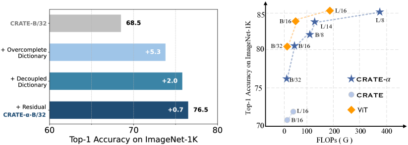
Figure 1: (Left) We demonstrate how modifications to the components enhance the performance of the crate model on ImageNet-1K. Details are provided in Section 3. (Right). We compare the FLOPs and accuracy on ImageNet-1K of our methods with ViT [8] and CRATE [41]. CRATE is trained only on ImageNet-1K, while crate-$\alpha$ and ViT are pre-trained on ImageNet-21K. The values of crate-$\alpha$ model correspond to those presented in Table 1.

To this end, this paper provides the first exploration of training crate at different scales for vision, i.e., Tiny, Small, Base, Large, Huge. Detailed model specifications are given in Table 4 of Appendix A. To achieve effective scaling, we make two key changes. First, we identify the vanilla ISTA block within crate as a limiting factor that hinders further scaling. To overcome this, we significantly expand the channels, decouple the association matrix, and add a residual connection, resulting in a new model variant — crate-$\alpha$. It is worth noting that this architecture change still preserves the mathematical interpretability of the model. Second, we propose an improved training recipe, inspired by previous work [33, 41, 34], for better coping the training with our new crate-$\alpha$ architecture.

We provide extensive experiments supporting the effective scaling of our crate-$\alpha$ models. For example, we scale the crate-$\alpha$ model from Base to Large size for supervised image classification on ImageNet-21K [5], achieving 85.1% top-1 accuracy on ImageNet-1K at the Large model size. We further scale the model size from Large to Huge, utilizing vision-language pre-training with contrastive learning on DataComp1B [9], and achieve a zero-shot top-1 accuracy of 72.3% on ImageNet-1K at the Huge model size. These results demonstrate the strong scalability of the crate-$\alpha$ model, shedding light on scaling up mathematically interpretable models for future work.

The main contributions of this paper are threefold:

1. We design three strategic yet minimal modifications for the crate model architecture to unleash its potential. In Figure 1, we reproduce the results of the crate model within our training setup, initially pre-training on ImageNet-21K classification and subsequently fine-tuning on ImageNet-1K classification. Compared to the vanilla crate model that achieves 68.5% top-1 classification accuracy on ImageNet-1K, our crate-$\alpha$-B/32 model significantly improves the vanilla crate model by 8%, which clearly demonstrates the benefits of the three modifications to the existing crate model. Moreover, following the settings of the best crate model and changing the image patch size from 32 to 8, our crate-$\alpha$-B model attains a top-1 accuracy of 83.2% on ImageNet-1K, exceeding the previous best crate model’s score of 79.5% by a significant margin of 3.7%.

2. Through extensive experiments, we show that one can effectively scale crate-$\alpha$ via model size and data simultaneously. In contrast, when increasing the crate model from Base to Large model size, there is a marginal improvement on top-1 classification accuracy (+0.5%, from 70.8% to 71.3%) on ImageNet-1K, indicating diminished returns [41]. Furthermore, by scaling the training dataset, we achieved a substantial 1.9% improvement in top-1 classification accuracy on ImageNet-1K, increasing from 83.2% to 85.1% when going from crate-$\alpha$ Base to Large.

3. We further successfully scale crate-$\alpha$ model from Large to Huge by leveraging vision-language pre-training on DataComp1B. Compared to the Large model, the Huge model (crate-$\alpha$-H) achieves a zero-shot top-1 classification accuracy of 72.3% on ImageNet-1K, marking a significant scaling gain of 2.5% over the Large model. These results indicate that the crate architecture has the potential to serve as an effective backbone for vision-language foundation models.

Related Work

White-box Transformers. [41, 40] argued that the quality of a learned representation can be assessed through a unified objective function called the sparse rate reduction. Based on this framework, [41, 40] developed a family of transformer-like deep network architectures, named crate, which are mathematically fully interpretable. crate models has been demonstrably effective on various tasks, including vision self-supervised learning and language modeling [23, 40]. Nevertheless, it remains unclear whether crate can scale as effectively as widely used black-box transformers. Previous work [41] suggests that scaling the vanilla crate model can be notably challenging.

Scaling ViT. ViT [8] represents the initial successful applications of Transformers to the image domain on a large scale. Many works [11, 27, 29, 28, 4, 32, 18, 19, 26, 15, 43] have deeply explored various ways of scaling ViTs in terms of model size and data size. From the perspective of self-supervision, MAE [11] provides a scalable approach to effectively training a ViT-Huge model using only ImageNet-1K. Following the idea of MAE, [27] further scales both model parameters to billions and data size to billions of images. Additionally, CLIP was the first to successfully scale ViT on a larger data scale (i.e., 400M) using natural language supervision. Based on CLIP, [28, 29] further scale the model size to 18 billion parameters, named EVA-CLIP-18B, achieving consistent performance improvements with the scaling of ViT model size. From the perspective of supervised learning, [43, 4] present a comprehensive analysis of the empirical scaling laws for vision transformers on image classification tasks, sharing some similar conclusions with [14]. [43] suggests that the performance-compute frontier for ViT models, given sufficient training data, tends to follow a saturating power law. More recently, [4] scales up ViT to 22 billion parameters. Scaling up different model architectures is non-trivial. [32, 18, 19] have made many efforts to effectively scale up different architectures. In this paper, due to the lack of study on the scalability of white-box models, we explore key architectural modifications to effectively scale up white-box transformers in the image domain.

2 Background and Preliminaries

In this section, we present the background on white-box transformers proposed in [41], including representation learning objectives, unrolled optimization, and model architecture. We first introduce the notation that will be used in the later presentation.

Notation. We use notation and problem setup following Yu et al. [41]. We use the matrix-valued random variable $\bm{X}=[\bm{x}_{1},\dots,\bm{x}_{N}]\in\mathbb{R}^{D\times N}$ to represent the data, where each $\bm{x}_{i}\in\mathbb{R}^{D}$ is a “token”, such that each data point is a realization of $\bm{X}$. For instance, $\bm{X}$ can represent a collection of image patches for an image, and $\bm{x}_{i}$ is the $i$-th image patch. We use $f\in\mathcal{F}\colon\mathbb{R}^{D\times N}\to\mathbb{R}^{d\times N}$ to denote the mapping induced by the transformer, and we let $\bm{Z}=f(\bm{X})=\begin{bmatrix}\bm{z}_{1},\dots,\bm{z}_{N}\end{bmatrix}\in\mathbb{R}^{d\times N}$ denote the features for input data $\bm{X}$. Specifically, $\bm{z}_{i}\in\mathbb{R}^{d}$ denotes the feature of the $i$-th input token $\bm{x}_{i}$. The transformer $f$ consists of multiple, say $L$, layers, and so can be written as $f=f^{L}\circ\cdots\circ f^{1}\circ f^{\textrm{pre}}$, where $f^{\ell}\colon\mathbb{R}^{d\times N}\to\mathbb{R}^{d\times N}$ denotes the $\ell$-th layer of the transformer, and the pre-processing layer is denoted by $f^{\textrm{pre}}=\mathbb{R}^{D\times N}\to\mathbb{R}^{d\times N}$. The input to the $\ell$-th layer $f^{\ell}$ of the transformer is denoted by $\bm{Z}^{\ell}=\begin{bmatrix}\bm{z}_{1}^{\ell},\dots,\bm{z}_{N}^{\ell}\end{bmatrix}\in\mathbb{R}^{d\times N}$, so that $f^{\ell}\colon\bm{Z}^{\ell}\mapsto\bm{Z}^{\ell+1}$. In particular, $\bm{Z}^{1}=f^{\textrm{pre}}(\bm{X})\in\mathbb{R}^{d\times N}$ denotes the output of the pre-processing layer and the input to the first layer.

2.1 Sparse Rate Reduction

Following the framework proposed in [40], we posit that the goal of representation learning is to learn a feature mapping or representation $f\in\mathcal{F}\colon\mathbb{R}^{D\times N}\to\mathbb{R}^{d\times N}$ that transforms the input data $\bm{X}$ (which may have a nonlinear, multi-modal, and otherwise complicated distribution) into structured and compact features $\bm{Z}$, such that the token features lie on a union of low-dimensional subspaces, say with orthonormal bases $\bm{U}_{[K]}=(\bm{U}_{k})_{k\in[K]}\in(\mathbb{R}^{d\times p})^{K}$. [41] proposes the Sparse Rate Reduction (SRR) objective to measure the goodness of such a learned representation:

$$\max_{f\in\mathcal{F}}\,\mathbb{E}_{\bm{Z}=f(\bm{X})}\left[L_{\texttt{srr}}(\bm{Z})\right]=\min_{f\in\mathcal{F}}\,\mathbb{E}_{\bm{Z}=f(\bm{X})}\left[R^{c}(\bm{Z}\,|\,\bm{U}_{[K]})-R(\bm{Z}\,|\,\bm{U}_{[K]})+\lambda\|\bm{Z}\|_{1}\right],$$ (1)

where $\bm{Z}=f(\bm{X})$ denotes the token representation, $\|\bm{Z}\|_{1}$ denotes the $\ell^{1}$ norm, and $R(\bm{Z})$, $R^{c}(\bm{Z}\,|\,\bm{U}_{[K]})$ are (estimates for) rate distortions [3, 6], defined as:

$$R(\bm{Z})\doteq\frac{1}{2}\log\det\left(\bm{I}+\frac{d}{N\epsilon^{2}}\bm{Z}^{\top}\bm{Z}\right),\qquad R^{c}(\bm{Z}\mid\bm{U}_{[K]})\doteq\sum_{k=1}^{K}R(\bm{U}_{k}^{\top}\bm{Z}).$$ (2)

In particular, $R^{c}(\bm{Z}\mid\bm{U}_{[K]})$ (resp. $R(\bm{Z})$) provide closed-form estimates for the number of bits required to encode the sample $\bm{Z}$ up to precision $\epsilon>0$, conditioned (resp. unconditioned) on the samples being drawn from the subspaces with bases $\bm{U}_{[K]}$. Minimizing the term $R^{c}$ improves the compression of the features $\bm{Z}$ against the posited model, and maximizing the term $R$ promotes non-collapsed features. The remaining term $\lambda\|\bm{Z}\|_{1}$ promotes sparse features. Refer to [40] for more details about the desiderata and objective of representation learning via the rate reduction approach.

2.2 crate: Coding RATE Transformer

Unrolled optimization. To optimize the learning objective and learn compact and structured representation, one approach is unrolled optimization [10, 31]: each layer of the deep network implements an iteration of an optimization algorithm on the learning objective. For example, one can design the layer $f^{\ell}$ such that the forward pass is equivalent to a proximal gradient descent step for optimizing learning objective $L(\bm{Z})$, i.e., $\bm{Z}^{\ell+1}=f^{\ell}(\bm{Z}^{\ell})=\texttt{Prox}[\bm{Z}^{\ell}-\eta\cdot\nabla_{\bm{Z}}L(\bm{Z}^{\ell})]$. Here we use $\eta$ to denote the step size and $\texttt{Prox}[\cdot]$ to denote the proximal operator [24].

One layer of the crate model. We now present the design of each layer of the white-box transformer architecture – Coding RATE Transformer (crate) – proposed in [41]. Each layer of crate contains two blocks: the compression block and the sparsification block. These correspond to a two-step alternating optimization procedure for optimizing the sparse rate reduction objective (1). Specifically, the $\ell$-th layer of crate is defined as

$$\bm{Z}^{\ell+1}=f^{\ell}(\bm{Z}^{\ell})={\texttt{ISTA}(\bm{Z}^{\ell+1/2}\,|\,\bm{D}^{\ell})},\quad\mathrm{where}\quad\bm{Z}^{\ell+1/2}=\bm{Z}^{\ell}+\operatorname{\texttt{MSSA}}(\bm{Z}^{\ell}).$$ (3)

Compression block (MSSA). The compression block in crate, called Multi-head Subspace Self-Attention block ($\operatorname{\texttt{MSSA}}$), is derived for compressing the token set $\bm{Z}=[\bm{z}_{1},\dots,\bm{z}_{N}]$ by optimizing the compression term $R^{c}$ (defined Eq. (1)), i.e.,

$$\bm{Z}^{\ell+1/2} =\bm{Z}^{\ell}+\operatorname{\texttt{MSSA}}(\bm{Z}^{\ell}\mid\bm{U}_{[K]}^{\ell})\approx\bm{Z}^{\ell}-\kappa\nabla_{\bm{Z}}R^{c}(\bm{Z}^{\ell}\,|\,\bm{U}_{[K]}^{\ell}),$$ (4)

where $\bm{U}_{[K]}^{\ell}$ denotes the (local) signal model at layer $\ell$, and the $\operatorname{\texttt{MSSA}}$ operator is defined as

$$\operatorname{\texttt{MSSA}}(\bm{Z}\mid\bm{U}_{[K]})=\frac{\kappa p}{N\epsilon^{2}}\,[\bm{U}_{1}\,\cdots\,\bm{U}_{K}]\begin{bmatrix}(\bm{U}_{1}^{\top}\bm{Z})\operatorname{softmax}((\bm{U}_{1}^{\top}\bm{Z})^{\top}(\bm{U}_{1}^{\top}\bm{Z}))\\ \vdots\\ (\bm{U}_{K}^{\top}\bm{Z})\operatorname{softmax}((\bm{U}_{K}^{\top}\bm{Z})^{\top}(\bm{U}_{K}^{\top}\bm{Z}))\end{bmatrix}.$$ (5)

Compared with the commonly used attention block in transformer [37], where the $k$-th attention head is defined as $(\bm{V}_{k}^{\top}\bm{Z})\operatorname{softmax}((\bm{Q}_{k}^{\top}\bm{Z})^{\top}(\bm{K}_{k}^{\top}\bm{Z}))$, $\operatorname{\texttt{MSSA}}$ uses only one matrix to obtain the query, key, and value matrices in the attention: that is, $\bm{U}_{k}=\bm{Q}_{k}=\bm{K}_{k}=\bm{V}_{k}$.

Sparse coding block (ISTA). The Iterative Shrinkage-Thresholding Algorithm (ISTA) block is designed to optimize the sparsity term and the global coding rate term, $\lambda\|\bm{Z}\|_{0}-R(\bm{Z}\mid\bm{U}_{[K]})$ in (1). [41] shows that an optimization strategy for these terms posits a (complete) incoherent dictionary $\bm{D}^{\ell}\in\mathbb{R}^{d\times d}$ and takes a proximal gradient descent step towards solving the associated LASSO problem $\mathop{\mathrm{arg\,min}}_{\bm{Z}\geq\bm{0}}[\frac{1}{2}\|{\bm{Z}^{\ell+1/2}-\bm{D}^{\ell}\bm{Z}}\|_{2}^{2}+\lambda\|{\bm{Z}}\|_{1}]$, obtaining the iteration

$$\bm{Z}^{\ell+1} =\texttt{ISTA}(\bm{Z}^{\ell+1/2}\,|\,\bm{D}^{\ell})=\mathrm{ReLU}(\bm{Z}^{\ell+1/2}+\eta\,(\bm{D}^{\ell})^{\top}(\bm{Z}^{\ell+1/2}-\bm{D}^{\ell}\bm{Z}^{\ell+1/2})-\eta\lambda\mathbf{1}).$$ (6)

In particular, the ISTA block sparsifies the intermediate iterates $\bm{Z}^{\ell+1/2}$ w.r.t. $\bm{D}^{\ell}$ to obtain $\bm{Z}^{\ell+1}$.

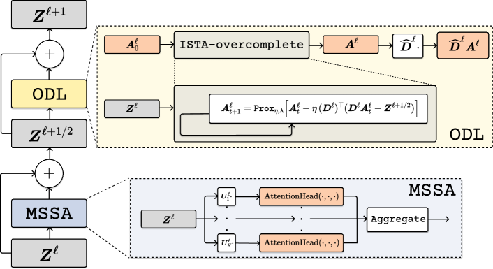
Figure 2: One layer of the crate-$\alpha$ model architecture. $\operatorname{\texttt{MSSA}}$ (Multi-head Subspace Self-Attention, defined in (5)) represents the compression block, and ODL (Overcomplete Dictionary Learning, defined in (12)) represents the sparse coding block.

3 CRATE-$\alpha$ Model

In this section, we present the crate-$\alpha$ architecture, which is a variant of crate [41]. As shown in Fig. 1 (Right), there is a significant performance gap between the white-box transformer crate-B/16 (70.8%) and the vision transformer ViT-B/16 (84.0%) [8]. One possible reason is that the ISTA block applies a complete dictionary $\bm{D}\in\mathbb{R}^{d\times d}$, which may limit its expressiveness. In contrast, the MLP block in the transformer applies two linear transformations $\bm{W}_{1},\bm{W}_{2}\in\mathbb{R}^{d\times 4d}$, leading to the MLP block having 8 times more parameters than the ISTA block.

Since the ISTA block in CRATE applies a single incremental step to optimize the sparsity objective, applying an orthogonal dictionary can make it ineffective in sparsifying the token representations. Previous work [25] has theoretically demonstrated that overcomplete dictionary learning enjoys a favorable optimization landscape. In this work, we use an overcomplete dictionary in the sparse coding block to promote sparsity in the features. Specifically, instead of using a complete dictionary $\bm{D}^{\ell}\in\mathbb{R}^{d\times d}$, we use an overcomplete dictionary $\bm{D}^{\ell}\in\mathbb{R}^{d\times(Cd)}$, where $C>1$ (a positive integer) is the overcompleteness parameter. Furthermore, we explore two additional modifications to the sparse coding block that lead to improved performance for crate. We now describe the three variants of the sparse coding block that we use in this paper.

Modification #1: Overparameterized sparse coding block. For the output of the $\ell$-th crate attention block $\bm{Z}^{\ell+1/2}$, we propose to sparsify the token representations with respect to an overcomplete dictionary $\bm{D}^{\ell}\in\mathbb{R}^{d\times(Cd)}$ by optimizing the following LASSO problem,

$$\bm{A}^{\ell}\approx\mathop{\mathrm{arg\,min}}_{\bm{A}\geq\bm{0}}\Big{[}\frac{1}{2}\|{\bm{Z}^{\ell+1/2}-\bm{D}^{\ell}\bm{A}}\|_{2}^{2}+\lambda\|{\bm{A}}\|_{1}\Big{]}.$$ (7)

To approximately solve (7), we apply two steps of proximal gradient descent, i.e.,

$$\bm{A}_{0}^{\ell}=\bm{0},\qquad\bm{A}^{\ell}_{1}=\texttt{Prox}_{\eta,\lambda}\big{[}\bm{A}^{\ell}_{0};\bm{D}^{\ell},\bm{Z}^{\ell+1/2}\big{]},\qquad\bm{A}^{\ell}_{2}=\texttt{Prox}_{\eta,\lambda}\big{[}\bm{A}^{\ell}_{1};\bm{D}^{\ell},\bm{Z}^{\ell+1/2}\big{]},$$ (8)

where Prox is the proximal operator of the above non-negative LASSO problem (7) and defined as

$$\texttt{Prox}_{\eta,\lambda}[\bm{A};\bm{D},\bm{Z}]=\operatorname{ReLU}(\bm{A}-\eta\bm{D}^{\top}(\bm{D}\bm{A}-\bm{Z})-\eta\lambda\bm{1}).$$ (9)

The output of the sparse coding block is defined as

$$\bm{Z}^{\ell+1}=\bm{D}^{\ell}\bm{A}^{\ell},\quad\mathrm{where}\quad\bm{A}^{\ell}=\bm{A}^{\ell}_{2}\doteq\texttt{ISTA-OC}(\bm{Z}^{\ell+1/2}\mid\bm{D}^{\ell}).$$ (10)

Namely, $\bm{A}^{\ell}$ is a sparse representation of $\bm{Z}^{\ell+1/2}$ with respect to the overcomplete dictionary $\bm{D}^{\ell}$. The original crate ISTA tries to learn a complete dictionary $\bm{D}\in\mathbb{R}^{d\times d}$ to transform and sparsify the features $\bm{Z}$. By leveraging more atoms than the ambient dimension, the overcomplete dictionary $\bm{D}\in\mathbb{R}^{d\times(Cd)}$ can provide a redundant yet expressive codebook to identify the salient sparse structures underlying $\bm{Z}$. As shown in Fig. 1, the overcomplete dictionary design leads to $5.3\%$ improvement compared to the vanilla crate model.

Modification #2: Decoupled dictionary. We propose to apply a decoupled dictionary $\widehat{\bm{D}}^{\ell}$ in the last step (defined in (10) of the sparse coding block, $\bm{Z}^{\ell+1}=\widehat{\bm{D}}^{\ell}\bm{A}^{\ell}$, where $\widehat{\bm{D}}^{\ell}\in\mathbb{R}^{d\times(Cd)}$ is a different dictionary compared to $\bm{D}^{\ell}$. By introducing the decoupled dictionary, we further improve the model performance by $2.0\%$, as shown in Fig. 1. We denote this mapping from $\bm{Z}^{\ell+1/2}$ to $\bm{Z}^{\ell+1}$ as the Overcomplete Dictionary Learning block (ODL), defined as follows:

$$\texttt{ODL}(\bm{Z}^{\ell+1/2}\mid\bm{D}^{\ell},\widehat{\bm{D}}^{\ell})\doteq\widehat{\bm{D}}^{\ell}\cdot\texttt{ISTA-OC}(\bm{Z}^{\ell+1/2}\mid\bm{D}^{\ell})=\widehat{\bm{D}}^{\ell}\bm{A}^{\ell}.$$ (11)

Modification #3: Residual connection. Based on the previous two modifications, we further add a residual connection, obtaining the following modified sparse coding block:

$$\bm{Z}^{\ell+1}=\bm{Z}^{\ell+1/2}+\texttt{ODL}(\bm{Z}^{\ell+1/2}\mid\bm{D}^{\ell},\widehat{\bm{D}}^{\ell}).$$ (12)

An intuitive interpretation of this modified sparse coding block is as follows: instead of directly sparsifying the feature representations $\bm{Z}$, we first identify the potential sparse patterns present in $\bm{Z}$ by encoding it over a learned dictionary. Subsequently, we incrementally refine $\bm{Z}$ by exploiting the sparse codes obtained from the previous encoding step. From Fig. 1, we find that the residual connection leads to a $0.7\%$ improvement.

To summarize, to effectively scale white-box transformers, we implement three modifications to the vanilla white-box crate model proposed in [41]. Specifically, in our crate-$\alpha$ model, we introduce a decoupling mechanism, quadruple the dimension of the dictionary (4$\times$), and incorporate a residual connection in the sparse coding block.

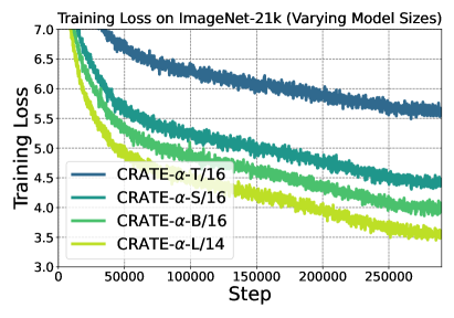
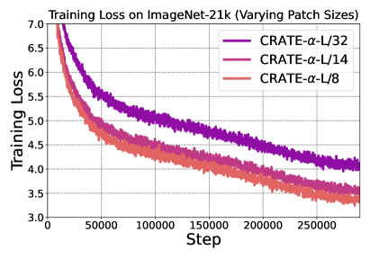
Figure 3: Training loss curves of crate-$\alpha$ on ImageNet-21K. (Left) Comparing training loss curves across crate-$\alpha$ with different model sizes. (Right) Comparing training loss curves across crate-$\alpha$-Large with different patch sizes.

4 Experiments

To thoroughly explore the scalability of crate-$\alpha$ model, we investigate its scaling behaviors from Base to Large size, and ultimately to Huge size. In the previous work [41], the largest model provided is Large size. Thus, for scaling to the Huge model, specifically our crate-$\alpha$-H configuration, we mainly follow the settings of the ViT [8]. For the transition from Base to Large size, we pre-train our model on ImageNet-21K and fine-tune it on ImageNet-1K via supervised learning. When scaling from Large to Huge, we utilize the DataComp1B [9] dataset within a vision-language pre-training paradigm. This allows us to study the effects of scaling the model to a massive size.

4.1 Scaling the crate-$\alpha$ Model from Base to Large

Dataset and evaluation. The standard ImageNet-21K dataset encompasses 21k classes and 14 million images. However, due to data loss, our version of the ImageNet-21K dataset is comprised of 19k classes and 13 million images. We believe that this minor discrepancy does not significantly affect the experimental results. Additionally, during pre-training on ImageNet-21K, we randomly allocated 1% of the data as a validation set to timely monitor the pre-training process. After pre-trained on ImageNet-21K, we further fine-tune the models on ImageNet-1K. We then evaluate the performance of these models on the ImageNet-1K validation set.

Training & fine-tuning. We initially pre-train the crate-$\alpha$ model on ImageNet-21K and subsequently fine-tune it on ImageNet-1K. During the pre-training phase, we set the learning rate to $8\times 10^{-4}$, weight decay to 0.1, and batch size to 4096. We apply data augmentation techniques such as Inception crop [30] resized to 224 and random horizontal flipping. In the fine-tuning phase, we adjust the base learning rate to $1.6\times 10^{-4}$, maintain weight decay at 0.1, and batch size at 4096. We apply label smoothing with a smoothing parameter of 0.1 and apply data augmentation methods including Inception crop, random horizontal flipping, and random augmentation with two transformations (magnitude of 9). For evaluation, we resize the smaller side of an image to 256 while maintaining the original aspect ratio and then crop the central portion to 224$\times$224. In both the pre-training and fine-tuning phases, we use the AdamW optimizer [21] and incorporate a warm-up strategy, characterized by a linear increase over 10 epochs. Both the pre-training and fine-tuning are conducted for a total of 91 epochs, utilizing a cosine decay schedule.

Results and analysis. As shown in Table  1, we compare crate-$\alpha$-B and crate-$\alpha$-L at patch sizes 32, 16, and 8. Firstly, we find our proposed crate-$\alpha$-L consistently achieves significant improvements across all patch sizes. Secondly, compared with the results of the vanilla crate (the first row of Table  1), increasing from crate-B to crate-L results in only a 0.5% improvement on ImageNet-1K. This indicates a case of diminishing returns. These findings compellingly highlight that the scalability of crate-$\alpha$ models significantly outperforms that of the vanilla crate. Meanwhile, the training loss in the pre-training stage is presented in Fig. 3; as the model capacity increases, the trend of the training loss improves predictably. This phenomenon is also described in [8].

Table 1: Top-1 accuracy of crate-$\alpha$ on ImageNet-1K with different model scales when pre-trained on ImageNet-21K and then fine-tuned on ImageNet-1K. For comparison, we also list the results from the paper [41] which demonstrate the diminished return from crate base to large, trained only on ImageNet-1K. "IN-21K" refers to ImageNet-21K. (^‡Results from [41].)

Models (Base)	ImageNet-1K(%)	Models (Large)	ImageNet-1K(%)
crate-B/16 w/o IN-21K	70.8‡	crate-L/16 w/o IN-21K	71.3‡
crate-$\alpha$-B/32	76.5	crate-$\alpha$-L/32	80.2
crate-$\alpha$-B/16	81.2	crate-$\alpha$-L/14	83.9
crate-$\alpha$-B/8	83.2	crate-$\alpha$-L/8	85.1

4.2 Scaling the crate-$\alpha$ Model from Large to Huge

Dataset and evaluation. In this part, we further increase the scale of the crate-$\alpha$ model to a Huge size. Building upon the insights from [8], the data-intensive nature of transformers poses significant challenges when attempting to scale vision transformers to a massive model size on ImageNet-21K. Thus, [8] utilizes the JFT-300M dataset to further scale the size of the training data. Since JFT-300M is not publicly accessible, we utilize a larger open dataset, DataComp1B [9]. This new state-of-the-art multimodal dataset, containing 1.4 billion image-text pairs, allows us to further scale our model to a massive size. Specifically, we train crate-$\alpha$ models using a contrastive learning-based approach, following the CLIP [26] paradigm. This enables us to observe scaling benefits when increasing the model size from Large to Huge. Considering the substantial computational requirements of training vanilla CLIP [26], we train the CLIP-like model following the CLIPA [15] protocol, which significantly reduces computational resources while maintaining competitive performance relative to CLIP. For evaluation, we evaluate the zero-shot accuracy of these models on ImageNet-1K.

Training & fine-tuning. In the pre-training stage, we utilize an image size of 84$\times$84, and the maximum token length is 32, with a total of 2.56 billion training samples. During the fine-tuning stage, we increase the image size to 224$\times$224 while maintaining the maximum token length at 32, with a 512 million training samples. Here, the key distinction between the pre-training stage and the fine-tuning stage is the image size. A smaller image size results in a faster training speed. In the configurations of crate-$\alpha$-CLIPA-B, crate-$\alpha$-CLIPA-L, and crate-$\alpha$-CLIPA-H, we use the crate-$\alpha$ model as the vision encoder, and utilize the same pre-trained huge transformer model from CLIPA [15] as the text encoder. For both the pre-training and fine-tuning stages, we freeze the text encoder and only train the vision encoder, i.e., the crate-$\alpha$ model. As we will show in the later results, this setup effectively demonstrates the scaling behaviors of crate-$\alpha$ models in the image domain. Detailed hyperparameter settings can be found in Appendix A.

Results and analysis. From the results shown in Fig. 4, we find that: (1) crate-$\alpha$-CLIPA-L/14 significantly outperforms crate-$\alpha$-CLIPA-B/16 by 11.3% and 9.0% in terms of ImageNet-1K zero-shot accuracy during the pre-training and fine-tuning stages, respectively. The substantial benefit suggests that the quality of learned representation may be constrained by the model size. Therefore, increasing the model size effectively leverages larger amounts of data. (2) When continuing to scale up model size, we also observe that crate-$\alpha$-CLIP-H/14 continues to benefit from larger training datasets, outperforming crate-$\alpha$-CLIP-L/14 by 3.1% and 2.5% in terms of ImageNet-1K zero-shot accuracy during the pre-training and fine-tuning stages, respectively. This demonstrates the strong scalability of the crate-$\alpha$ model. To explore the performance ceiling, we train a standard ViT-CLIPA-H/14 from scratch and observe improved performance.

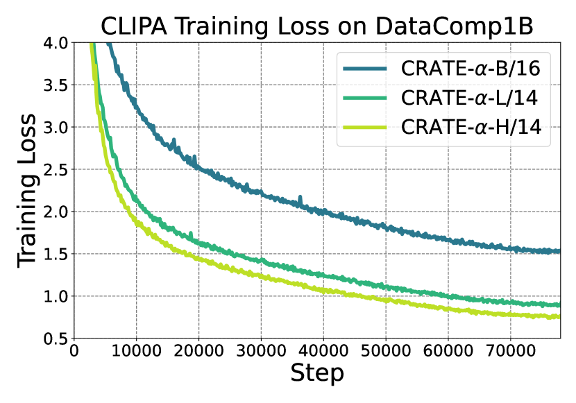
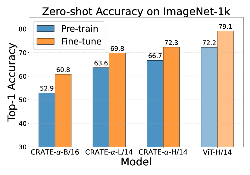
Figure 4: (Left) Comparing training loss curves of crate-$\alpha$-CLIPA with different model sizes on DataComp1B. (Right) Comparing zero-shot accuracy of crate-$\alpha$-B/L/H models and ViT-H on ImageNet-1K.

4.3 Compute-efficient Scaling Strategy

We further explore methods to scale models efficiently in terms of computation. Table 1 demonstrates that the crate-$\alpha$ model scales effectively from the Base model to its larger variants. However, the pre-training computation for the top-performing model, crate-$\alpha$-L/8, is resource-intensive on ImageNet-21K. Inspired by CLIPA [15], we aim to reduce computational demands by using reduced image token sequence lengths during the pre-training stage, while maintaining the same training setup during the fine-tuning stage. The results are summarized in Table 2.

Results and analysis. (1) When fine-tuning with crate-$\alpha$-L/14 and using crate-$\alpha$-L/32 for pre-training on ImageNet-21K, this approach consumes less than 30% of the TPU v3 core-hours required by crate-$\alpha$-L/14, yet achieves a promising 83.7% top-1 accuracy on ImageNet-1K, comparable to the 83.9% achieved by crate-$\alpha$-L/14; (2) When fine-tuning with crate-$\alpha$-L/8 and using crate-$\alpha$-L/32 for pre-training, this approach consumes just 10% of the training time required by crate-$\alpha$-L/8, yet it still achieves a promising 84.2% top-1 accuracy on ImageNet-1K, compared to 85.1% when using the crate-$\alpha$-L/8 model in the pre-training stage. In summary, we find that this strategy offers a valuable reference for efficiently scaling crate-$\alpha$ models in the future.

Table 2: Compute-efficient scaling strategy. To reduce the compute requirements of the pre-training stage, we use a model with a larger patch size. This results in a shorter token length for the same input size. The second column indicates the compute requirements of the pre-training stage, measured in TPU v3 core-hours. Details are provided in Section 4.3.

Model used in pre-train stage	TPU v3 core-hours	Fine-tuning model	ImageNet-1K(%)
crate-$\alpha$-L/32	2,652	crate-$\alpha$-L/14	83.7
		crate-$\alpha$-L/8	84.2
crate-$\alpha$-L/14	8,947	crate-$\alpha$-L/14	83.9
crate-$\alpha$-L/8	35,511	crate-$\alpha$-L/8	85.1

4.4 Improved Semantic Interpretability of crate-$\alpha$

As shown in previous subsections, crate-$\alpha$ can be effectively scaled up from Base to Huge when increasing the data size from millions to billions of images. In addition to scalability, we study the interpretability of our proposed crate-$\alpha$ with different model sizes. we follow the evaluation setup of crate in [41]. Specifically, we apply MaskCut [38] to validate and evaluate the rich semantic information captured by our model, including both qualitative and quantitative results.

As shown in Figure 5, we provide the segmentation visualization on COCO val2017 [17] for crate-$\alpha$, crate, and ViT, respectively. We find that our model preserves and even improves the (semantic) interpretability advantages of crate. Moreover, we summarize quantitative evaluation results on COCO val2017 in Table 3. Interestingly, when scaling up model size for crate-$\alpha$, the Large model improves over the Base model in terms of object detection and segmentation.

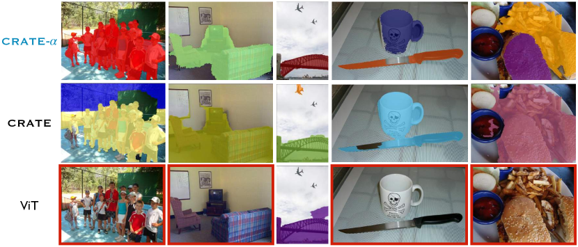
Figure 5: Visualization of segmentation on COCO val2017 [17] with MaskCut [38]. (Top row) Supervised crate-$\alpha$ effectively identifies the main objects in the image. Compared with crate (Middle row), crate-$\alpha$ achieves better segmentation performance in terms of boundary. (Bottom row) Supervised ViT fails to identify the main objects in most images. We mark failed image with  .

Table 3: Object detection and fine-grained segmentation via MaskCut on COCO val2017 [17]. We evaluate models of various scales and assess their average precision using COCO’s official evaluation metric. Compared with existing models such as crate and ViT, crate-$\alpha$ model achieves a notable performance gain. In addition, when scaling crate-$\alpha$ from base to large, it also exhibits the benefit of scalability.

		Detection			Segmentation
Model	Train	AP${}_{50}\uparrow$	AP${}_{75}\uparrow$	AP $\uparrow$	AP${}_{50}\uparrow$	AP${}_{75}\uparrow$	AP $\uparrow$
crate-B/8 [42]	Supervised	2.9	1.0	1.3	2.2	0.7	1.0
ViT-B/8 [42]	Supervised	0.8	0.2	0.4	0.7	0.5	0.4
crate-$\alpha$-B/8	Supervised	3.5	1.1	1.5	2.2	1.0	1.1
crate-$\alpha$-L/8	Supervised	4.0	1.7	2.0	2.7	1.1	1.4

5 Discussion

Limitations. Although we have used some existing compute-efficient training methods (e.g., CLIPA [15]) and have initiated an exploration into compute-efficient scaling strategies for white-box transformers in Section 4.3, this work still requires a relatively large amount of computational resources, which may not be easily accessible to many researchers.

Societal impact. A possible broader implication of this research is the energy consumption needed to conduct the experiments in our scaling study. But we believe understanding the scaling behaviors of white-box transformers is meaningful for practical purposes due to their mathematical and semantic interpretability. Additionally, our trained models can be used in various downstream tasks in the transfer learning setting, further amortizing the pre-training compute costs.

6 Conclusion

This paper provides the first exploration of training white-box transformer crate at scale for vision tasks. We introduce both principled architectural changes and improved training recipes to unleash the potential scalability of the crate type architectures. With these modifications, we successfully scale up the crate-$\alpha$ model along both the dimensions of model size and data size, while preserving, in most cases even improving, the semantic interpretability of the learned white-box transformer models. We believe this work provides valuable insights into scaling up mathematically interpretable deep neural networks, not limited to transformer-like architectures.

Acknowledgement

This work is supported by a gift from Open Philanthropy, TPU Research Cloud (TRC) program, and Google Cloud Research Credits program.

Appendix

Appendix A Additional Experiments and Details

Model configuration. We provide details about crate-$\alpha$ model configurations in Table 4.

Table 4: Model configurations for different sizes of crate-$\alpha$, parameter counts, and comparisons to crate models. $L$ is depth, $d$ is the hidden size, and $K$ is the number of heads.

Model Size	$L$	$d$	$K$	crate-$\alpha$ # Params	crate # Params
Tiny	12	192	3	4.8M	1.7M
Small	12	576	12	41.0M	13.1M
Base	12	768	12	72.3M	22.8M
Large	24	1024	16	253.8M	77.6M
Huge	32	1280	16	526.8M	159.8M

Training details of crate-$\alpha$-CLIPA models. When employing the crate-$\alpha$ architecture to replace the vision encoder in the CLIPA [15] framework, we essentially follow the original CLIPA training recipe. The setup for the pre-training stage is presented in Table 5. During the fine-tuning stage, we made some modifications: the input image size is set to $224\times 224$, the warmup steps are set to 800, and the base learning rate is set to 4e-7. When calculating the loss, we use the classification token from the vision encoder as the image feature and the last token from the text encoder as the text feature.

To explore the performance ceiling, we also train a ViT-CLIPA model from scratch. Most of the hyperparameters remain the same as those in Table 5, but there are some modifications in the pre-training stage. The batch size is set to 65,536, and the text length is set to 8 to speed up training. As with the CLIPA setup, warm-up steps are set to 3,200. Additionally, we add color jitter and grayscale augmentation, and use global average pooling instead of the classification token. These modifications help stabilize training.

Config	Value
optimizer	AdamW [22]
optimizer momentum	(0.9, 0.95)
batch size	32768
base lr	8e-6
minimal lr	0
warm-up steps	1600
schedule	cosine decay [20]
weight decay	0.2
random crop area	(40, 100)
resize method	bi-linear
temperature init	1/0.07 [12, 16]

Table 5: Pre-training hyper-parameters for CLIPA.

Visualization of self-attention maps of crate-$\alpha$. We provide visualization of attention maps of crate-$\alpha$ in Fig. 6.

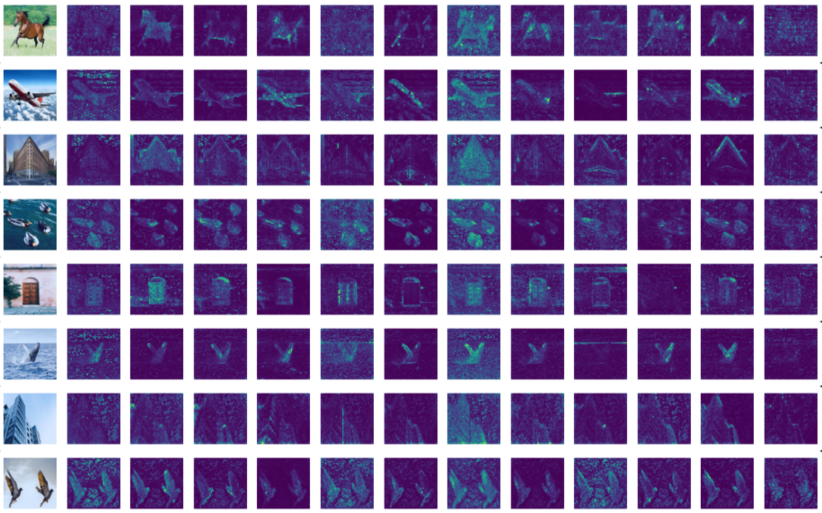
Figure 6: We visualize the self-attention maps of the crate-$\alpha$ Base model using $8\times 8$ patches trained using classification. Similar to the original CRATE [42], our model also demonstrates the capability to automatically capture the structural information of objects. For each row, the original image is displayed on the left, while the corresponding self-attention maps are shown on the right. The number of self-attention maps corresponds to the number of heads in the crate-$\alpha$ model.

Visualization of loss curves. We visualize the training loss curves of the four models, including crate and its three variants, in Fig. 7. We visualize the training loss curves of crate-$\alpha$-Base with different patch sizes in Fig. 8. In Fig. 9, we also visualize the training loss curves of models trained with efficient scaling strategy described in Section 4.3.

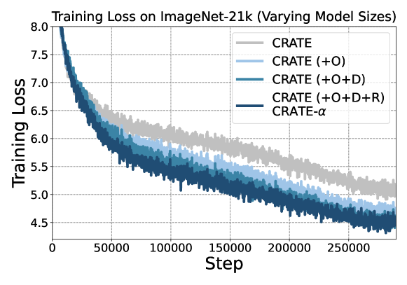
Figure 7: Training loss curves of different model architectures (mentioned in Fig. 1) on ImageNet-21K. The patch size is 32 for all four models shown in this figure. (+O: +overcomplete dictionary, +D: +decoupled dictionary, +R: +residual connection.)

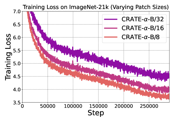
Figure 8: Comparing training loss curves across crate-$\alpha$-Base with different patch sizes.

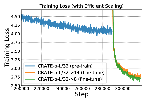
Figure 9: Comparing training loss curves when using the efficient scaling strategy. The blue curve corresponds to the crate-$\alpha$-Large/32 model (in the pre-training stage). After pre-training the crate-$\alpha$-Lage/32, we further fine-tune it with smaller patch sizes (longer token length), including patch size 14 (orange curve) and patch 8 (green curve).

References

- Blumensath and Davies [2008] Thomas Blumensath and Mike E Davies. Iterative thresholding for sparse approximations. Journal of Fourier analysis and Applications, 14:629–654, 2008.
- Brown et al. [2020] Tom Brown, Benjamin Mann, Nick Ryder, Melanie Subbiah, Jared D Kaplan, Prafulla Dhariwal, Arvind Neelakantan, Pranav Shyam, Girish Sastry, Amanda Askell, et al. Language models are few-shot learners. Advances in neural information processing systems, 33:1877–1901, 2020.
- Cover [1999] Thomas M Cover. Elements of information theory. John Wiley & Sons, 1999.
- Dehghani et al. [2023] Mostafa Dehghani, Josip Djolonga, Basil Mustafa, Piotr Padlewski, Jonathan Heek, Justin Gilmer, Andreas Peter Steiner, Mathilde Caron, Robert Geirhos, Ibrahim Alabdulmohsin, et al. Scaling vision transformers to 22 billion parameters. In International Conference on Machine Learning, pages 7480–7512. PMLR, 2023.
- Deng et al. [2009] Jia Deng, Wei Dong, Richard Socher, Li-Jia Li, Kai Li, and Li Fei-Fei. Imagenet: A large-scale hierarchical image database. In 2009 IEEE conference on computer vision and pattern recognition, pages 248–255. Ieee, 2009.
- Derksen et al. [2007] Harm Derksen, Yi Ma, Wei Hong, and John Wright. Segmentation of multivariate mixed data via lossy coding and compression. In Visual Communications and Image Processing 2007, volume 6508, pages 170–181. SPIE, 2007.
- Devlin et al. [2018] Jacob Devlin, Ming-Wei Chang, Kenton Lee, and Kristina Toutanova. Bert: Pre-training of deep bidirectional transformers for language understanding. arXiv preprint arXiv:1810.04805, 2018.
- Dosovitskiy et al. [2020] Alexey Dosovitskiy, Lucas Beyer, Alexander Kolesnikov, Dirk Weissenborn, Xiaohua Zhai, Thomas Unterthiner, Mostafa Dehghani, Matthias Minderer, Georg Heigold, Sylvain Gelly, et al. An image is worth 16x16 words: Transformers for image recognition at scale. arXiv preprint arXiv:2010.11929, 2020.
- Gadre et al. [2024] Samir Yitzhak Gadre, Gabriel Ilharco, Alex Fang, Jonathan Hayase, Georgios Smyrnis, Thao Nguyen, Ryan Marten, Mitchell Wortsman, Dhruba Ghosh, Jieyu Zhang, et al. Datacomp: In search of the next generation of multimodal datasets. Advances in Neural Information Processing Systems, 36, 2024.
- Gregor and LeCun [2010] Karol Gregor and Yann LeCun. Learning fast approximations of sparse coding. In Proceedings of the 27th international conference on international conference on machine learning, pages 399–406, 2010.
- He et al. [2022] Kaiming He, Xinlei Chen, Saining Xie, Yanghao Li, Piotr Dollár, and Ross Girshick. Masked autoencoders are scalable vision learners. In Proceedings of the IEEE/CVF conference on computer vision and pattern recognition, pages 16000–16009, 2022.
- Ilharco et al. [2021] Gabriel Ilharco, Mitchell Wortsman, Ross Wightman, Cade Gordon, Nicholas Carlini, Rohan Taori, Achal Dave, Vaishaal Shankar, Hongseok Namkoong, John Miller, Hannaneh Hajishirzi, Ali Farhadi, and Ludwig Schmidt. Openclip. July 2021.
- Jiang et al. [2023] Albert Q Jiang, Alexandre Sablayrolles, Arthur Mensch, Chris Bamford, Devendra Singh Chaplot, Diego de las Casas, Florian Bressand, Gianna Lengyel, Guillaume Lample, Lucile Saulnier, et al. Mistral 7b. arXiv preprint arXiv:2310.06825, 2023.
- Kaplan et al. [2020] Jared Kaplan, Sam McCandlish, Tom Henighan, Tom B Brown, Benjamin Chess, Rewon Child, Scott Gray, Alec Radford, Jeffrey Wu, and Dario Amodei. Scaling laws for neural language models. arXiv preprint arXiv:2001.08361, 2020.
- Li et al. [2024] Xianhang Li, Zeyu Wang, and Cihang Xie. An inverse scaling law for clip training. Advances in Neural Information Processing Systems, 36, 2024.
- Li et al. [2023] Yanghao Li, Haoqi Fan, Ronghang Hu, Christoph Feichtenhofer, and Kaiming He. Scaling language-image pre-training via masking. In CVPR, 2023.
- Lin et al. [2014] Tsung-Yi Lin, Michael Maire, Serge Belongie, James Hays, Pietro Perona, Deva Ramanan, Piotr Dollár, and C Lawrence Zitnick. Microsoft coco: Common objects in context. In Computer Vision–ECCV 2014: 13th European Conference, Zurich, Switzerland, September 6-12, 2014, Proceedings, Part V 13, pages 740–755. Springer, 2014.
- Liu et al. [2021] Ze Liu, Yutong Lin, Yue Cao, Han Hu, Yixuan Wei, Zheng Zhang, Stephen Lin, and Baining Guo. Swin transformer: Hierarchical vision transformer using shifted windows. In Proceedings of the IEEE/CVF international conference on computer vision, pages 10012–10022, 2021.
- Liu et al. [2022] Zhuang Liu, Hanzi Mao, Chao-Yuan Wu, Christoph Feichtenhofer, Trevor Darrell, and Saining Xie. A convnet for the 2020s. In Proceedings of the IEEE/CVF conference on computer vision and pattern recognition, pages 11976–11986, 2022.
- Loshchilov and Hutter [2017a] Ilya Loshchilov and Frank Hutter. Sgdr: Stochastic gradient descent with warm restarts. In ICLR, 2017a.
- Loshchilov and Hutter [2017b] Ilya Loshchilov and Frank Hutter. Decoupled weight decay regularization. arXiv preprint arXiv:1711.05101, 2017b.
- Loshchilov and Hutter [2018] Ilya Loshchilov and Frank Hutter. Decoupled weight decay regularization. In ICLR, 2018.
- Pai et al. [2023] Druv Pai, Ziyang Wu, Sam Buchanan, Tianzhe Chu, Yaodong Yu, and Yi Ma. Masked completion via structured diffusion with white-box transformers. In Conference on Parsimony and Learning (Recent Spotlight Track), 2023.
- Parikh et al. [2014] Neal Parikh, Stephen Boyd, et al. Proximal algorithms. Foundations and trends® in Optimization, 1(3):127–239, 2014.
- Qu et al. [2019] Qing Qu, Yuexiang Zhai, Xiao Li, Yuqian Zhang, and Zhihui Zhu. Geometric analysis of nonconvex optimization landscapes for overcomplete learning. In International Conference on Learning Representations, 2019.
- Radford et al. [2021] Alec Radford, Jong Wook Kim, Chris Hallacy, Aditya Ramesh, Gabriel Goh, Sandhini Agarwal, Girish Sastry, Amanda Askell, Pamela Mishkin, Jack Clark, et al. Learning transferable visual models from natural language supervision. In International conference on machine learning, pages 8748–8763. PMLR, 2021.
- Singh et al. [2023] Mannat Singh, Quentin Duval, Kalyan Vasudev Alwala, Haoqi Fan, Vaibhav Aggarwal, Aaron Adcock, Armand Joulin, Piotr Dollár, Christoph Feichtenhofer, Ross Girshick, et al. The effectiveness of mae pre-pretraining for billion-scale pretraining. In Proceedings of the IEEE/CVF International Conference on Computer Vision, pages 5484–5494, 2023.
- Sun et al. [2023] Quan Sun, Yuxin Fang, Ledell Wu, Xinlong Wang, and Yue Cao. Eva-clip: Improved training techniques for clip at scale. arXiv preprint arXiv:2303.15389, 2023.
- Sun et al. [2024] Quan Sun, Jinsheng Wang, Qiying Yu, Yufeng Cui, Fan Zhang, Xiaosong Zhang, and Xinlong Wang. Eva-clip-18b: Scaling clip to 18 billion parameters. arXiv preprint arXiv:2402.04252, 2024.
- Szegedy et al. [2015] Christian Szegedy, Wei Liu, Yangqing Jia, Pierre Sermanet, Scott Reed, Dragomir Anguelov, Dumitru Erhan, Vincent Vanhoucke, and Andrew Rabinovich. Going deeper with convolutions. In Proceedings of the IEEE conference on computer vision and pattern recognition, pages 1–9, 2015.
- Tolooshams and Ba [2021] Bahareh Tolooshams and Demba Ba. Stable and interpretable unrolled dictionary learning. arXiv preprint arXiv:2106.00058, 2021.
- Tolstikhin et al. [2021] Ilya O Tolstikhin, Neil Houlsby, Alexander Kolesnikov, Lucas Beyer, Xiaohua Zhai, Thomas Unterthiner, Jessica Yung, Andreas Steiner, Daniel Keysers, Jakob Uszkoreit, et al. Mlp-mixer: An all-mlp architecture for vision. Advances in neural information processing systems, 34:24261–24272, 2021.
- Touvron et al. [2021] Hugo Touvron, Matthieu Cord, Matthijs Douze, Francisco Massa, Alexandre Sablayrolles, and Hervé Jégou. Training data-efficient image transformers & distillation through attention. In International conference on machine learning, pages 10347–10357. PMLR, 2021.
- Touvron et al. [2022] Hugo Touvron, Matthieu Cord, and Hervé Jégou. Deit iii: Revenge of the vit. In European conference on computer vision, pages 516–533. Springer, 2022.
- Touvron et al. [2023a] Hugo Touvron, Thibaut Lavril, Gautier Izacard, Xavier Martinet, Marie-Anne Lachaux, Timothée Lacroix, Baptiste Rozière, Naman Goyal, Eric Hambro, Faisal Azhar, et al. Llama: Open and efficient foundation language models. arXiv preprint arXiv:2302.13971, 2023a.
- Touvron et al. [2023b] Hugo Touvron, Louis Martin, Kevin Stone, Peter Albert, Amjad Almahairi, Yasmine Babaei, Nikolay Bashlykov, Soumya Batra, Prajjwal Bhargava, Shruti Bhosale, et al. Llama 2: Open foundation and fine-tuned chat models. arXiv preprint arXiv:2307.09288, 2023b.
- Vaswani et al. [2017] Ashish Vaswani, Noam Shazeer, Niki Parmar, Jakob Uszkoreit, Llion Jones, Aidan N Gomez, Łukasz Kaiser, and Illia Polosukhin. Attention is all you need. Advances in neural information processing systems, 30, 2017.
- Wang et al. [2023] Xudong Wang, Rohit Girdhar, Stella X Yu, and Ishan Misra. Cut and learn for unsupervised object detection and instance segmentation. In Proceedings of the IEEE/CVF conference on computer vision and pattern recognition, pages 3124–3134, 2023.
- Wei et al. [2022] Jason Wei, Yi Tay, Rishi Bommasani, Colin Raffel, Barret Zoph, Sebastian Borgeaud, Dani Yogatama, Maarten Bosma, Denny Zhou, Donald Metzler, et al. Emergent abilities of large language models. Transactions on Machine Learning Research, 2022.
- Yu et al. [2023a] Yaodong Yu, Sam Buchanan, Druv Pai, Tianzhe Chu, Ziyang Wu, Shengbang Tong, Hao Bai, Yuexiang Zhai, Benjamin D Haeffele, and Yi Ma. White-box transformers via sparse rate reduction: Compression is all there is? arXiv preprint arXiv:2311.13110, 2023a.
- Yu et al. [2023b] Yaodong Yu, Sam Buchanan, Druv Pai, Tianzhe Chu, Ziyang Wu, Shengbang Tong, Benjamin Haeffele, and Yi Ma. White-box transformers via sparse rate reduction. Advances in Neural Information Processing Systems, 36, 2023b.
- Yu et al. [2024] Yaodong Yu, Tianzhe Chu, Shengbang Tong, Ziyang Wu, Druv Pai, Sam Buchanan, and Yi Ma. Emergence of segmentation with minimalistic white-box transformers. In Conference on Parsimony and Learning, pages 72–93. PMLR, 2024.
- Zhai et al. [2022] Xiaohua Zhai, Alexander Kolesnikov, Neil Houlsby, and Lucas Beyer. Scaling vision transformers. In Proceedings of the IEEE/CVF conference on computer vision and pattern recognition, pages 12104–12113, 2022.