Massless Quasiparticles in Bogoliubov-de Gennes Systems

Abstract

Gapless quasiparticles can exist in the Bogoliubov-de Gennes (BdG) Hamiltonians in the mean field description of superconductors (SCs), fermionic superfluids (SFs) and quantum spin liquids (QSLs). The mechanism of gapless quasiparticles in superconductors was studied in literature based on the homotopy theory or symmetry-indicators. However, important properties of the gapless quasiparticles including the degeneracy, the energy-momentum dispersion and the responses to external probe fields need to be determined. In the present work, we investigate gapless quasiparticles in general BdG systems by using projective representation theory for the full ‘symmetry’ groups formed by combinations of lattice, spin and charge operations. We found that (I) charge conjugation (or effective charge conjugation) symmetry can yield gapless quasiparticles with linear, quadratic or higher order dispersions at high symmetry points of the Brillouin zone; (II) different quantum numbers protected level crossing can give rise to zero modes along high symmetry lines; (III) combined spatial inversion and time reversal symmetry can protect zero modes appearing at generic $k$ point. To obtain the low energy properties of gapless quasiparticles, the $k\cdot p$ theory is provided using a high efficient method–the Hamiltonian approach. Based on generalized band representation theory for BdG systems, several lattice models are constructed to illustrate the above results. Our theory provides a method to classify nodal SCs/SFs/QSLs with given symmetries, and enlightens the realization of Majorana type massless quasiparticles in condensed matter physics.

I Introduction

In condensed matter physics, quasiparticle excitations emergent in the long-wave length limit behave like elementary particles in high energy physics. For instance, massless Dirac fermions or Weyl fermions can appear in semimetals at some points of the first Brillouin zone (BZ) if the crystal have certain space group symmetryWan et al. [2011], Fang et al. [2012], Wang et al. [2013], Yang and Nagaosa [2014], Weng et al. [2015], Ruan et al. [2016], Wu et al. [2020a]. These gapless quasiparticles result in observable physical consequences, such as the negative magnetic resistance effect or the existence of fermi arc spectrum in the surface excitationsNoh et al. [2017], Guo et al. [2019], Yang et al. [2019]. Furthermore, new types of quasiparticles having no counter part in high energy physics can exist in lattice systemsZyuzin and Burkov [2012], Hosur and Qi [2013], Xu et al. [2015]. The gapless quasi-particles are characterized by multiple degeneracy in the energy spectrum which carry projective representations (Reps) of their symmetry groupsYang and Liu [2017]. At a high symmetry point of the BZ, multiple degeneracy can be guaranteed by nontrivial irreducible (projective) Reps of the little co-group and around the degenerate point massless quasiparticle is formed Bradley and Davies [1968], Bradley and Cracknell [2010], Birman [2012], Hamermesh [2012]. For instance, at the K and K^′ points of the grapheneNovoselov et al. [2005] 2-fold degeneracy is protected by a 2-dimensional (2-D) Rep of the group $\mathscr{C}_{3v}$ and Dirac-like quasiparticles are formed with linear dispersion. Gapless quasiparticles can also result from symmetry protected level crossing of two bands along certain symmetric line of the BZ, in which case the quasiparticles carry reducible (projective) Reps of the little co-groupYoung and Kane [2015], Weng et al. [2016], Bouhon and Black-Schaffer [2017], Chang et al. [2017], Yu et al. [2019], Xiao et al. [2020]. A complete description and classification of the quasiparticles needs not only the projective Reps of the symmetry groups but only the symmetry invariants which label the classes of the projective Reps Chen et al. [2013], Yang et al. [2021a], Chen et al. [2023]. With the usage of symmetry invariants, many new types of quasiparticles are found in magnetically ordered systems having weak spin-orbit coupling Wu et al. [2020b], Yang et al. [2021b], Guo et al. [2022], Tang and Wan [2022] whose symmetry groups are dubbed spin space groupsJiang et al. [2023], Xiao et al. [2023], Ren et al. [2023]. Besides the gapless quasiparticles at distinct momentum points, nodal line/surface structures can be formed if the multiple degeneracy are ensured on a line/surface of the BZ Volovik [1993], Burkov et al. [2011], Phillips and Aji [2014], Fang et al. [2015], Kim et al. [2015], Mullen et al. [2015], Bzdušek et al. [2016], Ezawa [2016], Zhao et al. [2016], Chang and Yee [2017], Yan et al. [2017]. The dispersion of the quasiparticles around the nodal points or nodal lines is determined by the effective Hamiltonian called the $k\cdot p$ model Kane [1966], Chuang and Chang [1996], Gresch [2018], Jiang et al. [2021], Yang et al. [2021c]. The $k\cdot p$ Hamiltonian, as well as the responses theory of the quasiparticle to external probe fields such as electric fields, magnetic fields and strain, can be obtained from the projective Reps associated with the quasiparticles.

The quasiparticles in semimetals as discussed above have $U(1)$ charge (or particle number) conservation symmetry. Another class of quasiparticles are of Bogoliubov type when the fermions pair with each other to form Cooper pairs such that the $U(1)$ symmetry of the system breaks down to $Z_{2}$. In the BdG Hamiltonian of SCs/SFs or QSLs, the pairing between fermions yields a ‘particle-hole symmetry’ $\mathcal{P}$, which ensures that the energy spectrum is symmetric under the reflection over zero energy. Therefore, gapless Bogoliubov quasiparticles near the ‘fermi level’ (i.e. zero energy) are of special interesting science they determine the low-energy physical responses of the system. Due to the particle-hole symmetry $\mathcal{P}$, the degenerate point of the gapless quasiparticles in their energy spectrum are exactly locating at zero energy and are named zero modes (which are even-fold degenerate)Agterberg et al. [2017], Geier et al. [2020], Ono and Shiozaki [2022], Yuan et al. [2023]. For instance, $d$-wave SCs on square lattice contain zero modes at four points in the diagonal lines of the BZ, around which linearly dispersive quasiparticles arise. Especially, if charge conjugation symmetry $\mathcal{C}$ is preserved then the Bogoliubov quasiparticles are of Majorana type which are anti-particles of themselves. The ‘anti-particle’ and particle are related by charge conjugation symmetry $\mathcal{C}$ (or ‘particle-anti-particle exchange symmetry’ Bryan Gin-ge Chen [2019]). Unlike high-energy physics where Majorana fermions are massive, in condensed matter physics Majorna excitations at high symmetry points of the BZ can be massless (i.e. gapless) in $\mathcal{C}$-symmetric superconductors (SCs) or fermionic superfluids (SFs). Although Majorana zero modes (gapless chiral majorana edge states) can appear on the boundary of topological SCs/SFs, in the present work we focus on the bulk spectrum.

The previous studies of bulk zero modes were mainly from the topological point of view, such as $\mathbb{Z}_{2}$ or $\mathbb{Z}$ invariants or symmetry indicators Agterberg et al. [2017], Po et al. [2017], Bradlyn et al. [2017a], Ono and Watanabe [2018], Geier et al. [2020], Ono and Shiozaki [2022]. A comprehensive theory of gapless quasiparticles in BdG systems, including their physical response to external prob fields, is still lacking. In the present work, starting from the symmetry groups and their representation theory, we systematically study the mechanisms for the appearance of the zero modes in the bulk spectrum of SCs/SFs or QSLs, and provide a method to obtain the physical properties of the gapless quasiparticles. We prove a theorem that without (effective) charge conjugation symmetry any zero modes at a given momentum point can be adiabatically removed. If (effective) charge conjugation symmetry is present, then zero modes can stably exist at high symmetry points in a band representation (with a fixed degrees of freedom in the unit cell), and gapless quasiparticles can be formed with linear, quadratic or higher order dispersions. Two types of zero modes are defined, namely irreducible zero modes and reducible zero modes, according to the projective representations of the full little co-group. From this we not only know the degeneracy of the zero modes, but can also systematically construct the $k.p$ model and the response matrix of the gapless quasiparticles to probe fields. Finally we provide a scheme to classify point nodal SCs/SFs/QSLs for a given symmetry group. We remark that our conclusions hold for all Altland–Zirnbauer symmetry classes of BdG systemsZirnbauer [1996], Altland and Zirnbauer [1997]. Furthermore, when the ‘particle-hole symmetry’ $\mathcal{P}$ is considered, the application of representations is different from that of conventional symmetry groups since $\mathcal{P}$ is anti-commuting with the Hamiltonian.

The rest part of the paper is organized as follows. In section II, after a brief introduction of symmetry groups for fermionic BdG Hamiltonians, we derive the conditions for the appearance of zero modes in the bulk spectrum of SCs/SFs or QSLs. Then in section III, we provide an efficient method for obtaining the effective $k\cdot p$ model as well as the physical response to external prob fields for the gapless quasiparticles. Concrete lattice modes are provided in section IV to illustrate the results in the previous sections. Section V is devoted to a scheme for classification of point-node SCs/SFs/QSLs and a summary of the main results.

II Zero modes in the Bulk spectrum of general BdG systems

In metals and insulators, the symmetry group is commuting with the Hamiltonian. For instance, at momentum point $k$ the Hamiltonian $\mathscr{H}_{k}$ is commuting with the little co-group $G_{k}$, namely $\mathscr{H}_{k}G_{k}=G_{k}\mathscr{H}_{k}$, such that the eigenspace of each energy level $\varepsilon_{k}$ generally carry an irrep of $G_{k}$. However, BdG systems like SCs/SFs are characterized by their particle-hole symmetry ${\mathcal{P}}$ which is anti-commuting with the Hamiltonian $\mathcal{P}\mathscr{H}=-\mathscr{H}\mathcal{P}$ and maps the eigenspace of $\varepsilon$ to that of $-\varepsilon$, $\mathscr{H}\mathcal{P}|\varepsilon\rangle=-\mathcal{P}\mathscr{H}|\varepsilon\rangle=-\varepsilon\mathcal{P}|\varepsilon\rangle,$ namely $\mathcal{P}|\varepsilon\rangle\propto|-\varepsilon\rangle$. Therefore, generally we need to treat the direct sum of the eigenspaces of $\{\varepsilon,-\varepsilon\}$.

II.1 Symmetry operations

At mean field level, the Hamiltonian of a SC/SF/QSL reads

$$H=\sum_{i\neq j}\Big{(}t_{ij}c_{i}^{\dagger}c_{j}+\Delta_{ij}c_{i}^{\dagger}c_{j}^{\dagger}+{\rm h.c}\Big{)}+\sum_{i}\lambda_{i}c_{i}^{\dagger}c_{i},$$ (1)

which can be written in a matrix form in the Nambu bases $\Psi^{\dagger}=[C^{\dagger},C^{T}]$ with $C^{\dagger}=[c_{1}^{\dagger},c_{2}^{\dagger},...,c_{N}^{\dagger}]$ and $C^{T}=[c_{1},c_{2},...,c_{N}]$ ($N$ is the total number of the degrees of freedom), namely

$$H=\Psi^{\dagger}\mathscr{H}\Psi+h_{0},$$

with $h_{0}={1\over 2}\sum_{i}\lambda_{i}$, $\mathscr{H}^{\dagger}=\mathscr{H}$ and ${\rm Tr}\ \mathscr{H}=0$. In the following, we will briefly introduce the symmetry operations of the Hamiltonian (1) and divide them into three different kinds.

(1) Space-time symmetry described by space groups or magnetic space groups.
If $g$ is a spatial symmetry operation, then $gC^{\dagger}g^{-1}=C^{\dagger}u(g)$, namely, $gc_{i}^{\dagger}g^{-1}=\sum_{j=1}^{N}u_{ji}(g)c_{j}^{\dagger}$. The Hamiltonian is invariant under the action of $g$, $gHg^{-1}=H,$ or equivalently $U(g)\mathscr{H}U^{-1}(g)=\mathscr{H}$ with

$$U(g)=\left(\begin{matrix}u(g)&\\ &u^{*}(g)\end{matrix}\right).$$

For a SC without magnetic order, the symmetry group is a direct product of space group and the time reversal group $Z_{2}^{\mathcal{T}}=\{E,\mathcal{T}\}$, namely the type-II magnetic space group. Here $\mathcal{T}$ acts as $\mathcal{T}C^{\dagger}\mathcal{T}^{-1}=C^{\dagger}u(\mathcal{T})K$ and $U(\mathcal{T})K\mathscr{H}KU^{-1}(\mathcal{T})=U(\mathcal{T})\mathscr{H}^{*}U^{-1}(\mathcal{T})=\mathscr{H}$ with

$$U(\mathcal{T})K=\left(\begin{matrix}u(\mathcal{T})&\\ &u^{*}(\mathcal{T})\end{matrix}\right)K.$$

If the system contains magnetic order, then the symmetry group is generally a magnetic space group of type-I, type-III or type-IV.

(2) Internal symmetries in the spin and charge sectors.
For spin-1/2 fermions, the set of spin operations form a group $SU(2)_{s}$, and the set of charge operations form another group $SU(2)_{c}$. The action of the two $SU(2)$ groups can be clearly seen by performing an unitary transformation to the complete Nambu bases $\Psi^{\dagger}=[C_{\uparrow}^{\dagger},C_{\downarrow}^{\dagger},C_{\uparrow}^{T},C_{\downarrow}^{T}]$ into $\bar{\Psi}^{\dagger}=[C_{\uparrow}^{\dagger},C_{\downarrow}^{\dagger},C_{\downarrow}^{T},-C_{\uparrow}^{T}]$ where $C_{\sigma}^{\dagger}=[c_{1\sigma}^{\dagger},...,c_{L\sigma}^{\dagger}]$ with $\sigma=\uparrow,\downarrow$ and $L$ the number of sites.

In the new bases $\bar{\Psi}^{\dagger}$, a spin rotation in the $SU(2)_{\rm s}$ group acts as

$$\bar{\Psi}^{\dagger}\to\bar{\Psi}^{\dagger}I_{2}\otimes\exp\{-\mathrm{i}{\boldsymbol{\sigma}\over 2}\cdot\boldsymbol{n}\theta\}\otimes I_{L},$$ (2)

where the three Pauli matrices $\sigma_{x,y,z}$ are the generators of the spin transformations and $\boldsymbol{n}$ is the axis of the spin rotation and $\theta\in[0,2\pi]$ is the rotation angle. If the system is free of spin-orbit coupling(SOC), then the symmetry group of the system is then a direct product group of a space group (or a magnetic space group) and $SU(2)_{\rm s}$. For systems with non-negligible SOC, the spatial point group operations also act on the spin degrees of freedom. The resulting space groups are know as double groups.

On the other hand, a charge operation in the $SU(2)_{\rm c}$ group transforms as

$$\bar{\Psi}^{\dagger}\to\bar{\Psi}^{\dagger}\exp\{-\mathrm{i}{\boldsymbol{\tau}\over 2}\cdot\boldsymbol{m}\varphi\}\otimes I_{2L},$$ (3)

where the three Pauli matrices $\tau_{x,y,z}$ are the generators of charge transformations, and $\boldsymbol{m}$ is the axis of the charge rotation and $\varphi\in[0,2\pi]$ is the rotation angle. In electronic systems the $SU(2)_{\rm c}$ charge group generally breaks down to its subgroup.

Notice that the $SU(2)_{s}$ and $SU(2)_{c}$ groups are not completely independent, they share the same center $Z_{2}^{f}=\{E,P_{f}\}$ which is generated by the fermion parity $P_{f}=e^{-\mathrm{i}2\pi{{\boldsymbol{\tau}}\over 2}\cdot\boldsymbol{m}}\otimes I_{2}=I_{2}\otimes e^{-\mathrm{i}2\pi{{\boldsymbol{\sigma}}\over 2}\cdot\boldsymbol{n}}$. As a consequence, the internal symmetry operations form a $SO(4)$ group.

Sometimes it is convenient to go back to the original Nambu bases $\Psi^{\dagger}=[C_{\uparrow}^{\dagger},C_{\downarrow}^{\dagger},C_{\uparrow}^{T},C_{\downarrow}^{T}]$, where a spin $SU(2)_{\rm s}$ rotation (2) is given by

$$\Psi^{\dagger}\to\Psi^{\dagger}\exp\left(-\mathrm{i}{\tilde{\bm{\sigma}}\over 2}\cdot\bm{n}\theta\right)\otimes I_{L},$$ (4)

with the three generators

$$\tilde{\sigma}_{x}=\tau_{z}\otimes\sigma_{x},\ \tilde{\sigma}_{y}=I_{2}\otimes\sigma_{y},\ \tilde{\sigma}_{z}=\tau_{z}\otimes\sigma_{z}.$$

A charge $SU(2)_{\rm c}$ transformation (3) then takes the following form

$$\Psi^{\dagger}\to\Psi^{\dagger}\exp\{-\mathrm{i}{\tilde{\boldsymbol{\tau}}\over 2}\cdot\boldsymbol{m}\varphi\}\otimes I_{L},$$ (5)

with

$$\tilde{\tau}_{x}=-\tau_{y}\otimes\sigma_{y},\ \tilde{\tau}_{y}=\tau_{x}\otimes\sigma_{y},\ \tilde{\tau}_{z}=\tau_{z}\otimes I_{2}.$$

An important charge operation is the charge conjugation $\mathcal{C}$ that exchanges the creation operators with the annihilation operators, such as $\bar{\mathcal{C}}=e^{-\mathrm{i}{{\tau}_{x}\over 2}\pi}$ or $\bar{\mathcal{C}}=e^{-\mathrm{i}{{\tau}_{y}\over 2}\pi}$ in the new bases $\bar{\Psi}^{\dagger}$. Generally a charge conjugation is of order 4 with $\mathcal{C}^{2}=P_{f}$. In the original Nambu bases $\Psi^{\dagger}$ the charge conjugation takes the form of $\mathcal{C}=e^{-\mathrm{i}{\tilde{\tau}_{x}\over 2}\pi}$ or $\mathcal{C}=e^{-\mathrm{i}{\tilde{\tau}_{y}\over 2}\pi}$. A Hamiltonian is said to have charge conjugation symmetry if it is invariant under the charge conjugation transformation, namely $\hat{\mathcal{C}}H\hat{\mathcal{C}}^{-1}=\Psi^{\dagger}\mathcal{C}\mathscr{H}\mathcal{C}^{\dagger}\Psi=H,$ which requires

$$\mathcal{C}\mathscr{H}\mathcal{C}^{\dagger}=\mathscr{H}.$$ (6)

Since the charge conjugation exchanges creation operators with annihilation operators, to preserve the $\mathcal{C}$ symmetry we must have $\lambda_{i}=0$ for all sites. Therefore, charge conjugation symmetry is a very stringent constraint in condensed matter systems since it requires the chemical potential to be zero everywhere. If a charge conjugation is combined with operations in the spin or/and lattice sectors to form a symmetry operation, then we call it an effective charge conjugation symmetry.

For fermions carrying integer spin (such as the spinless fermions discussed in section IV.3) the charge group is simply $O(2)\cong U(1)\rtimes Z_{2}^{\mathcal{C}}$, where $U(1)=\{e^{-\mathrm{i}\tau_{z}\theta};\theta\in[0,2\pi)\}$ and $Z_{2}^{\mathcal{C}}=\{E,\tau_{x}\}$ is generated by the charge conjugation $\mathcal{C}=\tau_{x}$ Liu et al. [2010].

(3) The particle-hole ‘symmetry’.
Notice that in the complete Nambu bases one has $\Psi^{\dagger}=\Psi^{T}\Gamma_{x}$ with $\Gamma_{x}=\tau_{x}\otimes I_{N}$. Furthermore, the transpose of a fermion bilinear Hamiltonian gives rise to a minus sign (if $h_{0}=0$), so any BdG system has a particle-hole ‘symmetry’

$$\Gamma_{x}K\mathscr{H}K\Gamma_{x}=-\mathscr{H}.$$ (7)

Owing to (7), the energy spectrum has a reflection symmetry centered at $E=0$ and the eigenvalues $\pm\varepsilon$ appear in pairs. The particle-hole ‘symmetry’ operation $\hat{\mathcal{P}}=\Gamma_{x}K$ in (7) is anti-unitary in the first quantization formalism. Since $\hat{\mathcal{P}}^{2}=1$, the corresponding symmetry class is called the D-class.

For spin-1/2 systems with spin rotational symmetry, one can introduce the reduced Nambu bases $\psi^{\dagger}=[C_{\uparrow}^{\dagger},C_{\downarrow}^{T}]$. In the reduced Nambu bases, the charge SU(2) operations act as

$$\psi^{\dagger}\to\psi^{\dagger}\exp\{-\mathrm{i}{\boldsymbol{\tau}\over 2}\cdot\boldsymbol{m}\varphi\}\otimes I_{L}$$ (8)

and the particle-hole symmetry is defined as $\hat{\mathcal{P}}=\mathrm{i}\Gamma_{y}K$ with $\Gamma_{y}=\mathrm{i}\tau_{y}\otimes I_{L}$ and $\hat{\mathcal{P}}^{2}=-1$. This symmetry class is called the C-class.

Since $\hat{\mathcal{P}}$ is anti-unitary, it transforms momentum $\boldsymbol{k}$ to $-\boldsymbol{k}$. Hence in momentum space, $\hat{\mathcal{P}}$ is not necessarily a symmetry operation. However, the combination of $\hat{\mathcal{P}}$ and spatial inversion (or time reversal, et al) operation form an effective particle-hole symmetry at momentum point $\boldsymbol{k}$ which anti-commute with the Hamiltonian $\mathscr{H}_{k}$. In late discussion, we denote the effective particle-hole symmetry as $\tilde{\mathcal{P}}$ with $\tilde{\mathcal{P}}=\mathcal{I}\hat{\mathcal{P}}$ (or $\tilde{\mathcal{P}}=\mathcal{T}\hat{\mathcal{P}}$, et al).

A symmetry operation that commutes with the BdG Hamiltonian can be either the first kind or the second kind, or a combination of them. We write such an operation in a general form as $\alpha=\{s_{\alpha},c_{\alpha}||p_{\alpha}|t_{\alpha}\}$, where $s_{\alpha},c_{\alpha},p_{\alpha}$ respectively denote the spin, charge and lattice point group operations and $t_{\alpha}$ is a fractional translation. In later discussion, we will denote such group as $G_{f}$, the ‘fermionic’ group. When including the particle-hole ‘symmetry’, the full group will be denoted as $F_{f}=G_{f}+\mathcal{P}G_{f}$ with $\mathcal{P}^{2}=E$ or $\mathcal{P}^{2}=P_{f}$. Notice that the fermionic group $G_{f}$ is generally an extension of the space group of the lattice, and the latter is denoted as the ‘bosonic’ group $G_{b}$. For instance, in section IV.1, we will study the wallpaper group $G_{b}=p4gm\times Z_{2}^{\mathcal{T}}$ with generators $C_{4},\mathcal{T},\{\mathcal{M}_{x}|{1\over 2},{1\over 2}\}$. When ignoring the spin rotation symmetry and introducing the reduced Nambu bases, the corresponding fermionic group $G_{f}$ is generated by $C_{4}^{\prime}=(E||C_{4}),\mathcal{T}^{\prime}=(IK||\mathcal{T})$ and $\mathcal{M}_{x}^{\prime}=\{e^{-\mathrm{i}{\tau_{z}\over 2}\pi}||\mathcal{M}_{x}|{1\over 2},{1\over 2}\}$ satisfying ${\mathcal{T}^{\prime}}^{2}=1,{\mathcal{M}_{x}^{\prime}}^{2}=\{P_{f}||1,0\}$ and $G_{f}/Z_{2}^{f}=G_{b}$ (here the ^′ stands for lattice operations dressed by spin or/and charge operations) .

In the present work, we will not dwell on the structures of all possible fermionic groups $G_{f}$ for a given $G_{b}$ , we just distinguish two types of them: in the first type, $G_{f}$ is ‘diagonal’ in the particle-hole sector; in the second type (such as projective symmetry groups of $Z_{2}$ QSLs) $G_{f}$ contains symmetry operations that are non-diagonal in the particle-hole sector.

Usually, an eigen space of a Hamiltonian carries an irrep of the symmetry group. However, in BdG systems since the ‘particle-hole symmetry’ $\mathcal{P}$ is anti-commuting with the Hamiltonian, the relationship between the energy eigenstates and the irreps of the group $F_{f}$ is subtle. In the following subsections, we will discuss zero energy modes and nonzero energy modes separately.

II.2 Irreducible Zero modes

Here we systematically study the zero modes in BdG Hamiltonians. We will focus on the spectrum at given momentum $\bm{k}$. We denote the effective particle-hole operation as $\tilde{\mathcal{P}}$ and write the ‘true symmetry group’ as $G_{f}(k)$ which is formed by operations that are commuting with $\mathscr{H}_{k}$. Then the full little co-group $F_{f}(k)$ is formed, with $F_{f}(k)=G_{f}(k)+\tilde{\mathcal{P}}G_{f}(k)$. Suppose that $\mathscr{H}_{k}$ contain zero modes and assume that the zero modes span a Hilbert space $\mathcal{L}_{0}$. We first consider the ‘minimal’ set of zero modes, where $\mathcal{L}_{0}$ carries irreducible Rep $D(F_{f}(k))$ of $F_{f}(k)$.

The restriction of $D(F_{f}(k))$ to the subgroup $G_{f}(k)$ can only have two possibilities (see App.D): it is either an irrep or a direct sum of two irreps of $G_{f}(k)$. If $\mathcal{L}_{0}$ also carries an irrep of $G_{f}(k)$(namely if the restricted rep $D(G_{f}(k))$ is irreducible), then the zero modes are stable and are protected by symmetry. We call this set of zero modes as ‘irreducible’ zero modes. On the other hand, if $\mathcal{L}_{0}$ is a direct sum of two subspaces each carrying an irrep of $G_{f}(k)$, then the zero modes in $\mathcal{L}_{0}$ are accidental and are not symmetry protected. In this case, one can add a small perturbation to lift the zero modes without breaking any symmetry. The obtained eigen modes in $\mathcal{L}_{0}$ have nonzero energies and are called a set of ‘irreducible nonzero modes’ in later discussion.

However, different irreducible zero modes can couple to each other and form nonzero energy modes, which is described by the following theorem.

Theorem 1.

Every irrep $D(F_{f}(k))$ of a set of zero modes has a partner $D^{\prime}(F_{f}(k))$ with which the zero modes can couple to form nonzero energy modes, if the bases of both $D(F_{f}(k))$ and $D^{\prime}(F_{f}(k))$ are included in the system.

The proof is simple. If $\tilde{\mathcal{P}}$ is unitary, noticing $\tilde{\mathcal{P}}^{2}\in G_{f}(k)$, one can set $D^{\prime}(G_{f}(k))=D(G_{f}(k))$ and $D^{\prime}(\tilde{\mathcal{P}})=-D(\tilde{\mathcal{P}})$. Then the Hamiltonian coupling the two reps $D(F_{f}(k))$ and $D^{\prime}(F_{f}(k))$ reads $h(k)=\varepsilon_{k}\mu_{x}\otimes I,$ where $\mu_{m},m=x,y,z$ are the Pauli matrices acting on the $D(F_{f}(k))\oplus D^{\prime}(F_{f}(k))$ direct sum sector. If $\tilde{\mathcal{P}}$ is anti-unitary, one can choose $D^{\prime}(F_{f}(k))=D(F_{f}(k))$, then a possible Hamiltonian that couples the two reps $D(F_{f}(k))$ and $D^{\prime}(F_{f}(k))$ is $h(k)=\varepsilon_{k}\mu_{y}\otimes I.$

According to the theorem, the ‘protected’ zero modes at the given momentum point $k$ can be lifted if it is allowed to add more orbitals to the system to enlarge the Hilbert space. Consequently, the zero modes are either completely gapped out or moved to a different momentum point.

Suppose that the system contains more than one sets of irreducible zero modes at $k$. If they are not coupleable partners of each other, then these zero modes are symmetry protected and stable. Otherwise, if two sets of irreducible zero modes are coupleable partners of each other, then they can be lifted to finite energy by adiabatically adjusting the Hamiltonian without breaking any symmetry. In the next subsection, we will analyze the precise relation between $D(F_{f}(k))$ and its coupleable partner $D^{\prime}(F_{f}(k))$.

II.3 Minimal nonzero modes: $\{\varepsilon_{k},-\varepsilon_{k}\}$ with $\varepsilon_{k}\neq 0$

Now we discuss the modes having nonzero energy. Since $\tilde{\mathcal{P}}$ maps the $n$-dimensional ($n$-D) eigenspace of $\mathscr{H}_{k}$ with eigenvalue $\varepsilon_{k}$ to the one with eigenvalue $-\varepsilon_{k}$, we need to investigate the $2n$-D subspace $\mathcal{L}_{\pm\varepsilon}$ formed by the direct sum of the eigenspaces $\{\varepsilon_{k},-\varepsilon_{k}\}$ for $\varepsilon_{k}\neq 0$. This subspace $\mathcal{L}_{\pm\varepsilon}$ is called minimal if it cannot be divided into smaller sets of nonzero modes without breaking any symmetry. There are two possible types of minimal nonzero modes: (i) $\mathcal{L}_{\pm\varepsilon}$ carries an irreducible rep of $F_{f}(k)$ and is called a set of ‘irreducible’ nonzero modes (INZM); (ii) $\mathcal{L}_{\pm\varepsilon}$ carries a direct sum of two irreducible zero modes of $F_{f}(k)$, and $\mathcal{L}_{\pm\varepsilon}$ will be called a set of ‘reducible’ minimal nonzero modes (RMNZM).

Table 1: Reducible minimal nonzero modes for the space $D(F_{f}(k))\oplus D^{\prime}(F_{f}(k))$ of the group $F_{f}(k)=G_{f}(k)+\tilde{\mathcal{P}}G_{f}(k)$. ‘U’ stands for unitary and ‘A’ denotes anti-unitary. The situations for unitary $\tilde{\mathcal{P}}$ with $\eta_{\tilde{\mathcal{P}}}=1$ correspond to two sets of uncoupled irreducible zero modes.

$\tilde{\mathcal{P}}$	$G_{f}(k)$	$D(G_{f}(k))=D^{\prime}(G_{f}(k))$	$D(\tilde{\mathcal{P}})[D^{\prime}(\tilde{\mathcal{P}})]^{-1}$	condition for RMNZM
U	U	irreducible	$\eta_{\tilde{\mathcal{P}}}I$	​​​​ ​​​​ ​​​​ ​​​​ ​​​​​​​​ ​​​​ ​​​​ ​​​​ ​​​​ (1) $\eta_{\tilde{\mathcal{P}}}=-1$,   $D(F_{f}(k))\ncong D^{\prime}(F_{f}(k))$
	A	$\mathbb{R}$-class	$\eta_{\tilde{\mathcal{P}}}I$	​​​​ ​​​​ ​​​​ ​​​​ ​​​​​​​​ ​​​​ ​​​​ ​​​​ ​​​​ (2) $\eta_{\tilde{\mathcal{P}}}=-1$,    $D(F_{f}(k))\ncong D^{\prime}(F_{f}(k))$
		$\mathbb{C}$-class	$\eta_{\tilde{\mathcal{P}}}I$,  if $\{D(\tilde{\mathcal{P}}),\Omega_{z}\}\neq 0$	​​​​ ​​​​ ​​​​ ​​​​ ​​​​​​​​ ​​​​ ​​​​ ​​​​ ​​​​ (3) $\eta_{\tilde{\mathcal{P}}}=-1$,    $D(F_{f}(k))\ncong D^{\prime}(F_{f}(k))$
			$e^{\mathrm{i}\theta\Omega_{z}}$, if $\{D(\tilde{\mathcal{P}}),\Omega_{z}\}=0$	​​​​ ​​​​ ​​​​ ​​​​ ​​​​​​​​ ​​​​ ​​​​ ​​​​ ​​​​ (4) $\theta\in[0,2\pi)$,  ​​$D(F_{f}(k))\cong D^{\prime}(F_{f}(k))$
		$\mathbb{H}$-class	​​​​ $\eta_{\tilde{\mathcal{P}}}I$,   if $\{D(\tilde{\mathcal{P}}),\Omega_{n}\}\neq 0$ for any $\boldsymbol{n}$	​​​​ ​​​​ ​​​​ ​​​​ ​​​​​​​​ ​​​​ ​​​​ ​​​​ ​​​​ (5) $\eta_{\tilde{\mathcal{P}}}=-1$,    $D(F_{f}(k))\ncong D^{\prime}(F_{f}(k))$
			$e^{\mathrm{i}\theta\Omega_{\boldsymbol{n}}}$, if $\{D(\tilde{\mathcal{P}}),\Omega_{n}\}=0$ for some $\boldsymbol{n}$	(6) $\theta\in[0,2\pi)$, ${\boldsymbol{n}}\in S^{2}$, ​$D(F_{f}(k))\cong D^{\prime}(F_{f}(k))$
A	U	irreducible	$e^{\mathrm{i}\theta}I$	​​​​ ​​​​ ​​​​ ​​​​ ​​​​​​​​ ​​​​ ​​​​ ​​​​ ​​​​ (7) $\theta\in[0,2\pi)$,  ​​$D(F_{f}(k))\cong D^{\prime}(F_{f}(k))$

II.3.1 Irreducible nonzero modes

By definition, the supporting space $\mathcal{L}_{\pm\varepsilon}$ of irreducible nonzero modes forms an irrep $D(F_{f}(k))$. The restricted rep on $G_{f}(k)$, namely $D(G_{f}(k))$, must be reducible, otherwise it would gives rise to a set of irreducible zero modes. We adopt the eigenbases of the Hamiltonian for the irreducible nonzero modes which takes the form $h(k)=\varepsilon_{k}\mu_{z}\otimes I_{n}$, where $\mu_{z}$ is the third Pauli matrix whose eigenvalues $\pm 1$ respectively label the eigen spaces with positive and negative energy. In the induced bases, see App.D, the element $g\in G_{f}(k)$ is represented as

$$D(g)K_{s(g)}=\begin{pmatrix}M(g)&0\\ 0&M^{\prime}(g)\end{pmatrix}K_{s(g)},$$

where $M(g)K_{s(g)}$ and $M^{\prime}(g)K_{s(g)}={\omega_{2}(g,\tilde{\mathcal{P}})\over\omega_{2}(\tilde{\mathcal{P}},\tilde{\mathcal{P}}^{-1}g\tilde{\mathcal{P}})}K_{s(\tilde{\mathcal{P}})}M(\tilde{\mathcal{P}}^{-1}g\tilde{\mathcal{P}})K_{s(g\tilde{\mathcal{P}})}$ are two $n$-D irreps of $G_{f}(k)$, and $\tilde{\mathcal{P}}$ is represented as

$$D(\tilde{\mathcal{P}})K_{s(\tilde{\mathcal{P}})}=\begin{pmatrix}0&\omega_{2}(\tilde{\mathcal{P}},\tilde{\mathcal{P}})M(\tilde{\mathcal{P}}^{2})\\ I_{n}&0\end{pmatrix}K_{s(\tilde{\mathcal{P})}}.$$

II.3.2 Reducible minimal nonzero modes

We now consider the case in which $\mathcal{L}_{\pm\varepsilon}$ contains two irreps of $F_{f}(k)$ having the the same factor system, and we note them as $D(F_{f}(k))$ and $D^{\prime}(F_{f}(k))$ respectively. By definition, the ‘minimal nonzero modes’ requires that the restricted Reps $D(G_{f}(k))$ and $D^{\prime}(G_{f}(k))$ are irreducible. From Schur’s lemma, the restricted reps $D(G_{f}(k))$ and $D^{\prime}(G_{f}(k))$ must be equivalent such that they can couple to each other. That is, $D(G_{f}(k))\cong D^{\prime}(G_{f}(k))$. We thus assume that the bases have been adjusted such that

$$D(G_{f}(k))=D^{\prime}(G_{f}(k)).$$ (9)

Furthermore, as summarized in table 1, the ability of coupling between the two sets of irreducible zero modes further restricts the relation between $D(\tilde{\mathcal{P}})K_{s(\tilde{\mathcal{P}})}$ and $D^{\prime}(\tilde{\mathcal{P}})K_{s(\tilde{\mathcal{P}})}$. In later discussion, we define the unitary quantity

$$M=D(\tilde{\mathcal{P}})[D^{\prime}(\tilde{\mathcal{P}})]^{-1}$$

to denote the difference between $D(\tilde{\mathcal{P}})$ and $D^{\prime}(\tilde{\mathcal{P}})$. As shown in App.E, the $M$ is commuting with the restricted rep $D(G_{f}(k))$.

(I) $\tilde{\mathcal{P}}$ is unitary (chiral-like, e.g. $\tilde{\mathcal{P}}=\mathcal{TP}$)

(a) If $G_{f}(k)$ is unitary, then from Schur’s lemma one has $M=\eta_{\tilde{\mathcal{P}}}I_{n}$ with $\eta_{\tilde{\mathcal{P}}}$ a constant. Since $\tilde{\mathcal{P}}^{2}\in G_{f}(k)$, hence $[D(\tilde{\mathcal{P}})]^{2}=[D^{\prime}(\tilde{\mathcal{P}})]^{2}$, namely $\eta_{\tilde{\mathcal{P}}}^{2}=1$, $\eta_{\tilde{\mathcal{P}}}=\pm 1$, see App.E.1.1. When $\eta_{\tilde{\mathcal{P}}}=-1$, then $\mathcal{L}_{\pm\varepsilon}$ is indeed a set of reducible minimal nonzero modes. When $\eta_{\tilde{\mathcal{P}}}=1$, $\mathcal{L}_{\pm\varepsilon}$ contains two sets of irreducible zero modes uncoupled to each other.

(b) If $G_{f}(k)$ is anti-unitary, denote the maximum unitary subgroup of $G_{f}(k)$ as $H_{f}(k)$. Then there will be three different situations.

b1), When the restricted rep $D(G_{f}(k))$ is of the real class $\mathbb{R}$, then $M=\eta_{\tilde{\mathcal{P}}}I_{n}$ still holds with $\eta_{\tilde{\mathcal{P}}}=\pm 1$. The case with $\eta_{\tilde{\mathcal{P}}}=-1$ stands for RMNZM.

b2), When the $D(G_{f}(k))$ is of the complex class $\mathbb{C}$, then the restricted rep $D(H_{f}(k))$ is a direct sum of two non-equivalent irreps with dimension ${n\over 2}$. Suppose $\Omega_{z}$ is diagonal in this direct sum space and is represented as $\Omega_{z}=\omega_{z}\otimes I_{n\over 2}$ with $\omega_{z}$ the third pauli matrix. Then the unitary elements in the centralizer of the rep $D(G_{f}(k))$ can be written as $e^{\mathrm{i}\theta\Omega_{z}}=\cos\theta+\mathrm{i}\sin\theta\Omega_{z}$, see App.E.1.2, where $\theta\in[0,2\pi)$. So we have $M=e^{\mathrm{i}\theta_{0}\Omega_{z}}$ for some $\theta_{0}$ with a constraint,

$$e^{-\mathrm{i}\theta_{0}\Omega_{z}}D(\tilde{\mathcal{P}})=D(\tilde{\mathcal{P}})e^{\mathrm{i}\theta_{0}\Omega_{z}}.$$ (10)

If $\{D(\tilde{\mathcal{P}}),\Omega_{z}\}\neq 0$, then $\sin\theta_{0}=0$, so $\theta_{0}=0,\pi$. The case $\theta_{0}=\pi$ (yielding $M=-I_{n}$) stands for the RMNZM. If $\{D(\tilde{\mathcal{P}}),\Omega_{z}\}=0$, then $\theta_{0}\in[0,2\pi)$ and $D(F_{f}(k))$ and $D^{\prime}(F_{f}(k))$ are equivalent since they are related by a $U(1)$ transformation $\Psi^{\dagger}\to\Psi^{\prime{\dagger}}=\Psi^{\dagger}e^{-\mathrm{i}\Omega_{z}{\theta_{0}\over 2}}$, $D(\tilde{\mathcal{P}})\to D^{\prime}(\tilde{\mathcal{P}})=e^{-\mathrm{i}\Omega_{z}{\theta_{0}\over 2}}D(\tilde{\mathcal{P}})e^{\mathrm{i}\Omega_{z}{\theta_{0}\over 2}}=e^{-\mathrm{i}\Omega_{z}{\theta_{0}}}D(\tilde{\mathcal{P}})$. The two irreps can be coupled to form nonzero modes. For instance, when $\theta_{0}=0$ the Hamiltonian can be chosen as $h_{k}=\varepsilon_{k}\mu_{y}\otimes\Omega_{z}.$

b3), When $D(G_{f}(k))$ is of the quaternionic class $\mathbb{H}$, then the unitary elements in the centralizer of the $D(G_{f}(k))$ can be written as $e^{\mathrm{i}\theta\Omega_{n}}$ (with $\Omega_{n}=\boldsymbol{\omega}\cdot\boldsymbol{n}\otimes I_{n\over 2}$, $\boldsymbol{\omega}$ the three pauli matrices) for any $\boldsymbol{n}\in S^{2},\theta\in[0,2\pi)$, see App.E.1.2. So we have

$$M=e^{\mathrm{i}\theta_{0}\Omega_{\boldsymbol{n}_{0}}}.$$ (11)

for some $\theta_{0},\boldsymbol{n}_{0}$ with the following constraint

$$e^{-\mathrm{i}\theta_{0}\Omega_{\boldsymbol{n}_{0}}}D(\tilde{\mathcal{P}})=D(\tilde{\mathcal{P}})e^{\mathrm{i}\theta_{0}\Omega_{\boldsymbol{n}_{0}}}$$ (12)

If $\{D(\tilde{\mathcal{P}}),\Omega_{\boldsymbol{n}_{0}}\}\neq 0$ for any ${\boldsymbol{n}_{0}}\in S^{2}$ (for instance, when ${\rm Tr\ D(\tilde{\mathcal{P}})}\neq 0$), then only $\theta_{0}=0,\pi$ satisfies the relation (10). Then (11) reduces to $M=\eta_{\tilde{\mathcal{P}}}I_{n}$ with $\eta_{\tilde{\mathcal{P}}}=\pm 1$ and the case $\eta_{\tilde{\mathcal{P}}}=-1$ stands for RMNZM. If there exist some ${\boldsymbol{n}_{0}}$ such that $\{D(\tilde{\mathcal{P}}),\Omega_{\boldsymbol{n}_{0}}\}=0$, then $D(\tilde{\mathcal{P}})$ and $D^{\prime}(\tilde{\mathcal{P}})$ are related by an SU(2) transformation $\Psi^{\dagger}\to\Psi^{\prime{\dagger}}=\Psi^{\dagger}e^{-\mathrm{i}\Omega_{\boldsymbol{n}_{0}}{\theta_{0}\over 2}}$, $D(\tilde{\mathcal{P}})\to D^{\prime}(\tilde{\mathcal{P}})=e^{-\mathrm{i}\Omega_{\boldsymbol{n}_{0}}{\theta_{0}\over 2}}D(\tilde{\mathcal{P}})e^{\mathrm{i}\Omega_{\boldsymbol{n}_{0}}{\theta_{0}\over 2}}=e^{-\mathrm{i}\Omega_{\boldsymbol{n}_{0}}{\theta_{0}}}D(\tilde{\mathcal{P}})$. Hence, the two irreps $D(F_{f}(k)$ and $D^{\prime}(F_{f}(k))$ are equivalent, they can be coupled to form nonzero modes. For instance, when $\theta_{0}=0$ the Hamiltonian can be chosen as $h_{k}=\varepsilon_{k}\mu_{y}\otimes\Omega_{n}.$

(II) $\tilde{\mathcal{P}}$ is antiunitary(particle-hole like, e.g. $\tilde{\mathcal{P}}=\mathcal{I}\mathcal{P}$)
If $G_{f}(k)$ is anti-unitary, we can multiply $\tilde{\mathcal{P}}$ with an anti-unitary element $T_{0}\in G_{f}(k)$ to obtain a chiral-like symmetry operator $\tilde{\mathcal{P}}^{\prime}=\tilde{\mathcal{P}}T_{0}$, which has been discussed in case (I). Therefore, we only need to consider the case in which $G_{f}(k)$ is unitary. Eq. (9) indicates that the two irreps $D(F_{f}(k))$ and $D^{\prime}(F_{f}(k))$ are equivalent, and consequently $D^{\prime}(\tilde{\mathcal{P}})K=e^{-\mathrm{i}\theta}D(\tilde{\mathcal{P}})K$ with $\theta\in[0,2\pi)$, namely $M=e^{\mathrm{i}\theta}I_{n}$, see App.E.2. Now $\mathcal{L}_{\pm\varepsilon}$ is a set of RMNZM since there exist a Hamiltonian matrix $h_{k}=\varepsilon_{k}(\sin{\theta\over 2}\mu_{x}+\cos{\theta\over 2}\mu_{y})\otimes I_{n}$ which commutes with $\mathscr{D}(G_{f}(k))=D(G_{f}(k))\oplus D(G_{f}(k))$ and anti-commutes with $\mathscr{D}(\tilde{\mathcal{P}})K=D(\tilde{\mathcal{P}})\oplus e^{-\mathrm{i}\theta}D(\tilde{\mathcal{P}})K$.

II.4 Conditions for the existence of Zero modes

Now we consider BdG systems on the lattice having a symmetry group $G_{f}$, and assume that a fixed number of complex fermion bases (namely local Wannier orbitals) are placed in certain Wyckoff positions in the unit cell. According to App.C, for any given momentum $\bm{k}$, the rep of $F_{f}(k)$ can be read out from the generalized band representation, and then we can know whether there exist zero modes at the $\bm{k}$. If zero modes do exist, the degeneracy must be even because the dimension of the Hamiltonian $\mathscr{H}_{k}$ is even and the nonzero energy levels appear in pairs $\{\varepsilon,-\varepsilon\}$. In the following theorem 2 (see App.F for proof), however, we show that if the $G_{f}(k)$ is ‘diagonal’ in the particle-hole sector, only minimal nonzero modes are stable at a given momentum $\bm{k}$.

Theorem 2.

For any BdG system whose symmetry group $G_{f}(k)$ is ‘diagonal’ in the particle-hole sector, all zero modes at the momentum point $\bm{k}$ can be adiabatically removed without breaking any symmetry.

Hence, for non-interacting SCs/SFs whose symmetry groups are magnetic space groups, zero modes at high symmetry points/lines are not symmetry-protected. However, as shown in App.F.3, (effective) charge conjugation symmetry can change the energy spectrum. In App.G, we prove that at a given $\bm{k}$ having $\tilde{\mathcal{P}}$ symmetry, there always exists a (effective) charge-conjugation symmetry $\mathcal{C}$ that turns certain set of minimal nonzero modes into a set of zero modes, called the $\mathcal{C}$-minimal zero modes. This conclusion is summarized in the following theorem 3.

Theorem 3.

At a given $\tilde{\mathcal{P}}$-symmetric momentum $\boldsymbol{k}$ (i.e. $\tilde{\mathcal{P}}\in F_{f}(k)$) of an arbitrary BdG system, any minimal nonzero modes (except for one special case) located at the momentum $\bm{k}$ can be turned into zero modes by adding a single charge-conjugation symmetry to the original BdG system. The exception is when $\tilde{\mathcal{P}}$ is anti-unitary while $G_{f}(k)$ is unitary, and the irrep $D(F_{f}(k))$ carried by a set of irreducible nonzero modes is of $\mathbb{H}$ class. In that case, one needs two charge-conjugation operations anti-commuting with each other to gain zero modes.

The charge conjugation is the simplest charge operation that is non-diagonal in the particle-hole sector. The existence of zero modes in the above theorem can be generalized to other situations where the charge conjugation operation $\mathcal{C}$ is replaced by general non-diagonal charge operations. For instance, such charge operation can be an element $\mathcal{D}\in SU(2)_{c}$ with $\mathcal{D}^{3}=E$.

On the other hand, zero modes can also appear at unfixed momentum. For instance, a level crossing of irreducible nonzero modes carrying two nonequivalent reps of $G_{f}(k)$ can give rise to a set of zero modes, as stated in the following theorem 4.

Theorem 4.

On a high symmetry line of the BZ having a unitary symmetry $\mathcal{M}$, if the eigenspaces $\{\varepsilon,-\varepsilon\}$ of a minimal nonzero modes carry different quantum numbers (i.e. characters of irreps) of $\mathcal{M}$, then the level crossing of $\varepsilon,-\varepsilon$ gives rise to a set of stable zero modes whose momentum is not fixed.

According to the above theorems, gapless quasiparticles can be found under one of the following three situations:

(1) presence of (effective) charge-conjugation symmetry or symmetries such that the Hilbert space contains a set of irreducible zero modes or sets of uncoupled irreducible zero modes at high symmetry point $\boldsymbol{k}$.

(2) presence of level crossing of bands carrying different quantum numbers of certain unitary symmetry operation of a high symmetry line.

(3) occurrence of $\pi$-quantized Berry phase protected by ($\mathcal{I}^{\prime}\mathcal{T}^{\prime}$) symmetry with $(\mathcal{I}^{\prime}\mathcal{T}^{\prime})^{2}=1$. Here $\mathcal{I}^{\prime}$ and $\mathcal{T}^{\prime}$ respectively stand for the inversion operation and the time-reversal operation dressed by spin or/and charge operations.

The condition (1) can be verified using the band representation theory for SCs/SFs/QSLs provided in App.C. The last two conditions are illustrated via concrete lattice models in Sec.IV. Especially, the $\mathcal{I}^{\prime}\mathcal{T}^{\prime}$ symmetry enforced $\pi$-quantized Berry phase can give rise to nodal-point like quasiparticles in 2-dimensions and nodal-line structures in 3-dimensions. This is a topological origin of the zero modes (usually linear dispersive), and is closely related to the zero modes at general $\bm{k}$ points enforced by symmetry indicators Po et al. [2017], Bradlyn et al. [2017a], Ono and Watanabe [2018], Geier et al. [2020], Ono et al. [2021], Ono and Shiozaki [2022]. The (projective) representation theory of symmetry groups discussed in the present work provides a different and complementary mechanism to obtain zero modes and gapless quasiparticles.

III $k\cdot p$ theory and physical response

The existence of degenerate modes (zero modes) in the bulk energy spectrum can give rise to nodal point or nodal line structure. The dispersion around the nodal points or nodal lines are reflected in the effective Hamiltonian called $k\cdot p$ theory. In this section, we will adopt the Hamiltonian approach Yang et al. [2021c] to obtain the $k\cdot p$ theory for zero modes of general BdG Hamiltonians.

Above all, we define the ‘particle-hole rep’ of $F_{f}(k)$

$$D^{(\rm ph)}(g)=+1,\ \ D^{(\rm ph)}(g\tilde{\mathcal{P}})=-1,$$ (13)

with $g\in G_{f}(k)$. Here the complex conjugation $K_{s(g)}$ is hidden since the particle-hole rep is essentially a real rep.

III.1 $k\cdot p$ Hamiltonian

When the full symmetry group $F_{f}$ and the electron bases in the unit cell are given, the band representation $D(F_{f})$ of general BdG systems can be obtained (see App.C), from which the stable zero modes are known. Suppose the stable zero modes at momentum $\bm{k}$ span a Hilbert space $\mathcal{L}_{0}$. When projected onto $\mathcal{L}_{0}$, the effective low-energy BdG Hamiltonian reads

$$H_{\rm eff}=\sum_{\delta k}\Phi_{\boldsymbol{k}+\delta\boldsymbol{k}}^{\dagger}\Lambda({\delta\bm{k}})\Phi_{\boldsymbol{k}+\delta\boldsymbol{k}}=\sum_{\delta k}H_{\boldsymbol{k}+\delta\boldsymbol{k}},$$

where the $\Phi_{\boldsymbol{k}}$ is the basis of the zero modes, and $\Lambda(\delta\boldsymbol{k})$ is a Hermitian matrix $\Lambda^{\dagger}(\delta\boldsymbol{k})=\Lambda(\delta\boldsymbol{k})$. When summing over all the momentum variations, the total Hamiltonian should preserve the $F_{f}(k)$ symmetry, namely $\hat{g}\left(\sum_{\delta\boldsymbol{k}}H_{\boldsymbol{k}+\delta\boldsymbol{k}}\right)\hat{g}^{-1}=\left(\sum_{\delta\boldsymbol{k}}H_{\boldsymbol{k}+\delta\boldsymbol{k}}\right),$ for all $g\in F_{f}(k)$. Assuming $\hat{g}\Phi^{\dagger}(\boldsymbol{k}+\delta\boldsymbol{k})\hat{g}^{-1}=\Phi^{\dagger}(\boldsymbol{k}+g\delta\boldsymbol{k})D(g)K_{s(g)}$, then generally for any $g\in F_{f}(k)$ one has

$$D(g)K_{s(g)}\Lambda\left(\delta\boldsymbol{k}\right)K_{s(g)}D^{\dagger}(g)=D^{(\rm ph)}(g)\Lambda(g\delta\boldsymbol{k}),$$ (14)

where $D^{(\rm ph)}(g)$ is the 1-D particle-hole Rep of $F_{f}(k)$ defined in (13).

Starting from (14), we derive the formula to judge the dispersion relation of the BdG system in momentum space around the zero modes. For instance, we consider linear dispersion around $\boldsymbol{k}$, namely

$$\Lambda(\delta\boldsymbol{k})=\sum_{m=1}^{d}\delta k_{m}\Lambda^{m}+O(\delta k^{2}).$$ (15)

Here $\delta\boldsymbol{k}$ is a dual vector under the action of group $F_{f}(k)$, namely $\hat{g}\delta k_{m}=\sum_{n}D_{mn}^{(\bar{\rm v})}(h)\delta k_{n},$ where $(\bar{\rm v})$ is the dual Rep of the vector Rep $(\rm v)$ of the group $F_{f}(k)$. Notice that $\delta\boldsymbol{k}$ reverses its sign under the following actions: the time reversal $\mathcal{T}^{\prime}$ (anti-unitary), the spatial inversion $\mathcal{I}^{\prime}$ (unitary), the particle-hole transformation $\mathcal{P}$ (anti-unitary), hence,

$$D^{(\bar{\rm v})}(\mathcal{T}^{\prime})K=-1K,D^{(\bar{\rm v})}(\mathcal{I}^{\prime})=-1,D^{(\bar{\rm v})}(\mathcal{P})K=-1K.$$

(recall that the ^′ stands for lattice operations dressed by spin or/and charge operations.)

(I) $F_{f}(k)$ is unitary. If $F_{f}(k)$ is a unitary group, then for any $g\in F_{f}(k)$ one has

$$D(g)\Lambda^{n}D(g)^{\dagger}=\sum_{m}{D}_{mn}^{(\bar{\rm v}\times{\rm ph})}(g)\Lambda^{m}$$ (16)

with ${D}^{(\bar{\rm v}\times{\rm ph})}(g)\equiv D^{(\rm ph)}(g)D^{(\bar{\rm v})}(g)$. Thus, the existence of linear dispersion is determined by whether the product Rep $D(F_{f}(k))\otimes D^{*}(F_{f}(k))$ contains the linear Rep $D^{(\bar{\rm v}\times{\rm ph})}(F_{f}(k))$ or not. It can be judged from the quantity

$$a_{(\rm\bar{v}\times{\rm ph})}={1\over|F_{f}(k)|}\sum_{g\in F_{f}(k)}|\chi(g)|^{2}\cdot\chi^{(\rm v\times{\rm{\overline{ph}}})}(g)$$ (17)

where $\chi^{({\rm v}\times{\rm{\overline{ph}}})}(g)\equiv\chi^{({\rm v}\times{\rm ph})}(g)=\operatorname{Tr}[{D}^{(\bar{\rm v}\times{\rm ph})}(g)]^{*}$. If $a_{({\rm\bar{v}}\times{\rm ph})}=0$, then the dispersion must be of order higher than 1. If $a_{({\rm\bar{v}}\times{\rm ph})}\neq 0$, then the dispersion is linear, and one can always find Hermitian matrices $\Lambda^{m}$ satisfying the equation (16) noticing that the Rep $({\rm\bar{v}}\times{\rm ph})$ is real.

(II) $F_{f}(k)$ is anti-unitary. The matrices $\Lambda^{m}$ also carry dual vector rep of the group $F_{f}(k)$.

For any $g\in F_{f}(k)$, one has

$$D(g)K_{s(g)}\Lambda^{n}K_{s(g)}D(g)^{\dagger}=\sum_{m}\Lambda^{m}{D}_{mn}^{(\bar{\rm v}\times{\rm ph})}(g),$$ (18)

where ${D}^{(\bar{\rm v}\times{\rm ph})}(g)K_{s(g)}\equiv D^{(\rm ph)}(g)D^{(\bar{\rm v})}(g)K_{s(g)}$ is a real Rep of $F_{f}(k)$ hence the operator $K_{s(g)}$ can be hidden. Hence the existence of linear dispersion also depends on whether the product Rep $D(F_{f}(k))\otimes D^{*}(F_{f}(k))$ contains the Rep $D^{(\bar{\rm v}\times{\rm ph})}(F_{f}(k))$ or not, under the condition that the CG coefficients can be reshaped into hermitian matrices.

Select an anti-unitary operation $T_{0}\in F_{f}(k)$ and introduce the following matrices

$$\tilde{\Lambda}^{m}=\Lambda^{m}\cdot D^{\rm T}(T_{0}).$$

According to the Hamiltonian approachYang et al. [2021c], the symmetry condition (18) with $g=T_{0}$ and the hermitian condition $(\Lambda^{m})^{\dagger}=\Lambda^{m}$ are combined into a single symmetry condition of $\tilde{\Lambda}^{m}$ (called $\eta_{0}$-symmetry condition):

$$\big{(}\tilde{\Lambda}^{m}\big{)}^{\rm T}=\eta_{0}D(T_{0}^{2})\sum_{n}D^{(\bar{\rm v}\times{\rm ph})}_{nm}(T_{0})\tilde{\Lambda}^{n}.$$ (19)

with $\eta_{0}=\omega_{2}(T_{0},T_{0})$.

Therefore, when restricted to the $\eta_{0}$-symmetric subspace, one only needs to consider the unitary symmetries of $\tilde{\Lambda}^{m}$ as discussed in case (I). This is a relatively simpler since the unitary elements are represented in the $\mathbb{C}$ field. On the other hand, $\Lambda^{m}$ carry real representations of $G_{f}(k)$ so one need to treat them in the $\mathbb{R}$ field which is more complicated. This subtlety makes the Hamiltonian approach a method with a high efficiency.

Similar to Eq.(17), the existence of linear dispersion can be judged by the following quantity

$$a_{({\rm\bar{v}}\times{\rm ph})}= \frac{1}{|F_{f}(k)|}\sum_{u}\Big{[}|\chi(u)|^{2}\chi^{({\rm v}\times{\rm{\overline{ph}}})}(u)+$$

$$\omega_{2}\left(uT_{0},uT_{0}\right)\chi\big{(}\left(uT_{0}\right)^{2}\big{)}\chi^{({\rm v}\times{\rm{\overline{ph}}})}\left(uT_{0}\right)\Big{]},$$ (20)

where the sum $\Sigma_{u}$ runs over all unitary elements $u\in F_{f}(k)$, namely if $a_{({\rm\bar{v}}\times{\rm ph})}\neq 0$, the dispersion is linear, otherwise the dispersion is of order higher than 1. Notice that the character $\chi^{({\rm v}\times{\rm{\overline{ph}}})}\left(uT_{0}\right)$ in (III.1) is well-defined although $uT_{0}$ is anti-unitary, because the rep $({\rm v}\times{\rm{\overline{ph}}})$ is a real rep such that the allowed bases transformations can only be real orthogonal matrices which keep $\chi^{({\rm v}\times{\rm{\overline{ph}}})}\left(uT_{0}\right)$ invariant.

Now we discuss how to obtain the matrices $\Lambda^{m}$ or $\tilde{\Lambda}^{m}$ in the case $a_{({\rm\bar{v}}\times{\rm ph})}\neq 0$. Besides the $\eta_{0}$-symmetry condition (19), the symmetry constraints for unitary elements $u\in F_{f}(k)$ reads

$$D(u)\tilde{\Lambda}^{m}R^{\rm T}(u) =\sum_{n}D^{(\bar{\rm v}\times{\rm ph})}_{nm}(u)\tilde{\Lambda}^{n},$$ (21)

with $R(u)=D(T_{0})D^{*}(u)D^{\dagger}(T_{0}).$ If we consider the set of matrices $\tilde{\Lambda}^{m}$ as a single column vector $\tilde{\boldsymbol{\Lambda}}$ with $(\tilde{\boldsymbol{\Lambda}})_{(n-1)\times d^{2}+(\alpha-1)\times d+\beta}=(\tilde{\Lambda}^{n})_{\alpha\beta},$ then the above constrains (21) indicates that $\tilde{\boldsymbol{\Lambda}}$ carries identity rep of any unitary element $u\in F_{f}(k)$, namely

$$W(u)\tilde{\boldsymbol{\Lambda}}=\tilde{\boldsymbol{\Lambda}},$$ (22)

with $W(u)=D^{({\rm v}\times{\rm{\overline{ph}}})}(u)\otimes D(u)\otimes R(u).$ Furthermore, $W(T_{0})K\tilde{\boldsymbol{\Lambda}}=\tilde{\boldsymbol{\Lambda}}$ also holds where $T_{0}$ is represented as $W(T_{0})K=D^{({\rm v}\times{\rm{\overline{ph}}})}(T_{0})\otimes D(T_{0})\otimes D(T_{0})K$.

When projected to the $\eta_{0}$-symmetric space, the rep $W(u)$ becomes $W_{\eta_{0}}(u)\equiv{\rm{Proj}_{\eta_{0}}}W(u)$ with the matrix entries given by

$$[W_{\eta_{0}}(u)]_{m\gamma\rho,n\alpha\beta}={1\over 2}\Big{[}D_{mn}^{({\rm v}\times{\rm{\overline{ph}}})}(u)D_{\gamma\alpha}(u)R_{\rho\beta}(u)+$$

$$\ \ \ \ \eta_{0}\sum_{\lambda}D_{mn}^{({\rm v}\times{\rm{\overline{ph}}})}(uT_{0})D_{\gamma\beta}(u)R_{\rho\lambda}(u)D_{\lambda\alpha}\left((T_{0})^{2}\right)\Big{]}.$$

The above matrix $W_{\eta_{0}}(u)$ is not a rep for the group formed by all unitary elements $u\in F_{f}(k)$, but it does contain the identity rep for that group, which shows that the dispersion contains linear term. Then the $\Lambda^{m}$ can be obtained via the following procedure:
(1) Obtain the common eigenvectors of $W_{\eta_{0}}(u)$ with eigenvalue 1 for all unitary elements $u\in F_{f}(k)$. These eigenvectors span a Hilbert subspace $\mathcal{L}^{(I)}$.
(2) Project $W(T_{0})K$ into $\mathcal{L}^{(I)}$, and perform bases transformation such that $T_{0}$ is represented as $IK$ in $\mathcal{L}^{(I)}$. Then the new bases are all of the allowed $\tilde{\boldsymbol{\Lambda}}$.
(3) Reshape each of the new bases into three matrices $\tilde{\Lambda}^{x},\tilde{\Lambda}^{y},\tilde{\Lambda}^{z}$.
(4) Finally one has $\Lambda^{m}=\tilde{\Lambda}^{m}[D(T_{0})^{\rm T}]^{-1}$.

The above procedure can be applied to the 0-th order $k\cdot p$ terms, i.e., to judge if an irrep gives rise to a set of zero modes and nonzero modes. This can be done by replacing the rep $({\rm v}\times{\rm{\overline{ph}}})$ in eq.(III.1) with the identity rep or the particle-hole rep, namely, if $a_{I}=1,a_{\rm ph}=0$, then the rep corresponds to a set of irreducible zero modes; if if $a_{I}=1,a_{\rm ph}\neq 0$, then the rep corresponds to a set of irreducible nonzero modes, and the obtained $\Lambda$ matrices are independent symmetric perturbation Hamiltonians.

Similarly, one can obtain higher order $k\cdot p$ terms. For instance, the linear rep carried by the quadratic dispersion $k_{\alpha}k_{\beta}$ is shown in Tab.2, where the $l=0$ rep is the identity rep and the $l=2$ rep can be reduced to direct sum of lower dimensional irreps $(\mu_{1})+(\mu_{2})+...$. From the irreps $(\mu_{1}),(\mu_{2}),...$ one can construct the corresponding matrices $\Lambda^{(\mu_{1})m_{1}},...$ that constitute the effective Hamiltonian

$$H=\sum_{\mu,m}f^{(\mu)_{m}}(\delta k)\Lambda^{(\mu)m}+\delta{\bm{k}}\cdot\delta{\bm{k}}\ \Lambda^{(0)},$$

where $f^{(\mu)_{m}}(\delta k)$ is the $m$-th basis (a quadratic polynomial of $\delta k$) of the irrep $\mu$ and $\Lambda^{(0)}$ is the $l=0$ term.

Table 2: Linear Reps of the lattice rotation ($l$ stands for angular momentum), time reversal $\mathcal{T}^{\prime}$, spatial inversion $\mathcal{I}^{\prime}$, charge conjugation $\mathcal{C}$ and particle-hole transformation $\mathcal{P}$ carried by probe fields: chemical potential $\lambda$, momentum $\boldsymbol{k}$, electric field $\boldsymbol{E}$, magnetic field $\boldsymbol{B}$, quadratic dispersion $k_{\alpha}k_{\beta}$, strain field $\epsilon_{\alpha\beta}$, and so on. The last column is the ‘particle-hole rep’ of operations in $F_{f}(k)$.

Prob fields	$\lambda$	$\boldsymbol{E}$	$\boldsymbol{B}$	$\boldsymbol{k}$	$k_{\alpha}k_{\beta}$	$\epsilon_{\alpha\beta}$	$D^{\rm{(ph)}}$
rotation	$l=0$	$l=1$	$l=1$	$l=1$	$l=0,2$	$l=0,2$	$+1$
$\mathcal{T}^{\prime}$	$+1$	$+1$	$-1$	$-1$	$+1$	$+1$	$+1$
$\mathcal{I}^{\prime}$	$+1$	$-1$	$+1$	$-1$	$+1$	$+1$	$+1$
$\mathcal{C}$	$-1$	$+1$	$+1$	$+1$	$+1$	$+1$	$+1$
$\mathcal{P}$	$+1$	$+1$	$+1$	$-1$	$+1$	$+1$	$-1$

III.2 Physical properties

The above method can also be applied to study the physical properties of the quasiparticles, namely, the response to external fields $\boldsymbol{f}$, such as electric field $\boldsymbol{E}$, magnetic field $\boldsymbol{B}$, strain field $\epsilon_{\alpha\beta}$, and so on. As summarized in Tab.2, the prob fields carry linear reps of $g\in F_{f}(k)$, namely

$$gf_{\alpha}=\sum_{\beta}D_{\beta\alpha}^{(\mu)}(g)f_{\beta},$$

where $(\mu)$ is a linear rep of $F_{f}(k)$. Then in the low energy effective Hamiltonian, fermion bilinear terms should be added to the $k\cdot p$ model,

$$H^{\prime}=\sum_{\alpha}f_{\alpha}\Lambda_{\alpha}.$$

Similar to (18), one has $D(g)K_{s(g)}\Lambda_{\alpha}K_{s(g)}D(g)^{-1}=\sum_{\beta}D^{{\rm(ph)}\times(\mu)}_{\beta\alpha}(g)\Lambda_{\beta}$. The matrices $\Lambda_{\alpha}$ can be obtained using the method introduced in the previous subsection.

Due to the ‘particle-hole symmetry’ $\mathcal{P}$ and the effective charge conjugation symmetry $\mathcal{C}$, the response of the Bogoliubov quasiparticles to external field is different from quasiparticles in semimetals. For instance, the chemical potential $\lambda$ is a scaler field under space-time operations, but it does not carry an identity rep of the group $F_{f}^{c}(k)$, hence the response matrix $\Lambda_{0}$ is not simply an identity matrix. If $\mathcal{P}$ is represented as $\tau_{x}\otimes I$, then the response matrix $\Lambda_{0}$ for $\lambda$ takes the form $\tau_{z}\otimes I$. Hence changing the chemical potential may either shift the position of the nodal point or fully gap out the quasiparticle.

Generally, the external fields may give mass to the gapless quasiparticles. The resulting gapped state may have nontrivial topological properties, such as nontrivial Chern numbers. These information are maintained in $k\cdot p$ model and the response matrix mentioned above. In the following section, we will illustrate all of the above results by several concrete lattice models.

IV Lattice Models: gapless quasiparticles in BdG systems

In this section, we present four models in two-dimensional lattice systems to illustrate the mechanisms and methods proposed in the previous sections. The first three models discuss zero modes protected by an effective charge conjugation $\mathcal{C}$, while the fourth model is a mean field Hamiltonian of $Z_{2}$ QSLs in which the projective symmetry group contains symmetry elements that are non-diagonal in the particle-hole sector.

IV.1 Square lattice: $G_{b}=p4gm\times Z_{2}^{\mathcal{T}}$

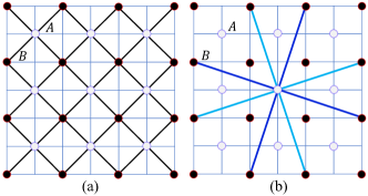
Figure 1: The model (23) with symmetry group $G_{b}=p4gm\times{Z}_{2}^{\mathcal{T}}$. (a) the hopping terms; (b) the pairing terms. The black and white circles stand for A and B sub-lattices respectively. The black bonds in (a) represent the hopping terms, and in (b), the cyan bonds stand for the phase $e^{\mathrm{i}\theta_{i,j}}=+1$ while the blue bonds stand for $e^{\mathrm{i}\theta_{i,j}}=-1$.

The first model is a spin-1/2 SC/SF of the CI class. We consider the square lattice with the magnetic wallpaper group $G_{b}=p4gm\times Z_{2}^{\mathcal{T}}$. On the 2a Wyckoff positions A=(0,0) and B=(${1\over 2},{1\over 2}$) with site group $\mathscr{C}_{4}\times Z_{2}^{\mathcal{T}}$, we place spin-1/2 fermionic orbitals $[c_{\uparrow}^{\dagger},c_{\downarrow}^{\dagger}]$. Assuming SOC is negligible, then the spin-1/2 fermion forms a Kramers doublet under time reversal $\mathcal{T}$ and is invariant under the site group rotation $\mathscr{C}_{4}$. Due to the SU(2) spin rotation symmetry, the BdG Hamiltonian can be written in the reduced Nambu bases $\psi_{i}^{\dagger}=[c_{{A}\uparrow}^{\dagger},c_{{B}\uparrow}^{\dagger},c_{{A}\downarrow},c_{{B}\downarrow}]_{i},$ where the symmetry group $G_{f}$ is generated by $C^{\prime}_{4}=C_{4},\mathcal{T}^{\prime}=(IK||\mathcal{T}),\mathcal{M}_{x}^{\prime}=\{e^{-\mathrm{i}{\tau_{z}\over 2}\pi}||\mathcal{M}_{x}|{1\over 2},{1\over 2}\}$ (here $e^{-\mathrm{i}{\tau_{z}\over 2}\pi}$ is a charge operation defined in (8)) and translation, with

$$\!\!\!\!\!\!\hat{C}_{4}\psi^{\dagger}_{i}\hat{C}_{4}^{-1}\!=\!\psi^{\dagger}_{C_{4}i},\ \ \ \hat{\mathcal{T}}^{\prime}\psi^{\dagger}_{i}\hat{\mathcal{T}}^{{}^{\prime}-1}\!=\!\psi^{\dagger}_{i}K,$$

$$\!\!\!\!\!\!\hat{\mathcal{M}}_{x}^{\prime}\psi^{\dagger}_{i}\hat{\mathcal{M}}_{x}^{{}^{\prime}-1}=$$

$$\mathrm{i}[c_{{B}\uparrow,\mathcal{M}_{x}i}^{\dagger},c_{{A}\uparrow,\mathcal{M}_{x}i+(0,1)}^{\dagger},-c_{{B}\downarrow,\mathcal{M}_{x}i},-c_{{A}\downarrow,\mathcal{M}_{x}i+(0,1)}].$$

Besides the particle-hole transformation

$$\hat{\mathcal{P}}\psi^{\dagger}_{i}\hat{\mathcal{P}}^{-1}=[c_{{A}\downarrow},c_{{B}\downarrow},-c_{{A}\uparrow}^{\dagger},-c_{{B}\uparrow}^{\dagger}]_{i}K,$$

we further consider an effective charge conjugation $\mathcal{C}=P_{f}^{B}e^{-\mathrm{i}{\tau_{y}\over 2}\pi}$ with $P_{f}^{B}[c_{A},c_{B}](P_{f}^{B})^{-1}=[c_{A},-c_{B}]$,

$$\widehat{\mathcal{C}}\psi^{\dagger}_{i}\widehat{\mathcal{C}}^{-1}=[c_{{A}\downarrow},-c_{{B}\downarrow},-c_{{A}\uparrow}^{\dagger},c_{{B}\uparrow}^{\dagger}]_{i},$$

and ${\widehat{\mathcal{C}}}^{2}=P_{f}$. Then we obtain the complete symmetry group $F^{c}_{f}$, whose band representation can be obtained according to App.C. Irreducible zero modes are found at $X=({1\over 2},0),Y=(0,{1\over 2}),M=({1\over 2},{1\over 2})$ points, where the $X$ and $Y$ points are related by $C^{\prime}_{4}$ symmetry.

To illustrate the above results, we consider a lattice model with inter-sublattice hopping and pairing terms,

$$H_{0} = {t\over 2}\sum_{\langle i_{\zeta},j_{\bar{\zeta}}\rangle}c_{i_{\zeta}\sigma}^{\dagger}c_{j_{\bar{\zeta}}\sigma}$$ (23)

$$+\Delta_{2}\!\!\sum_{\langle\langle i_{\zeta},j_{\bar{\zeta}}\rangle\rangle}\!\!e^{\mathrm{i}\theta_{i,j}}(c_{i_{\zeta}\uparrow}^{\dagger}c_{j_{\bar{\zeta}}\downarrow}^{\dagger}-c_{i_{\zeta}\downarrow}^{\dagger}c_{j_{\bar{\zeta}}\uparrow}^{\dagger})+{\rm h.c.}$$

where $\zeta=A,B$ and $\bar{\zeta}\neq\zeta$. The phase $e^{\mathrm{i}\theta_{i,j}}=\pm 1$ of the pairing term on the bond $(ij)$ alternatively equals to $1,-1$, as shown in Fig.1. After Fourier transformation, the Hamiltonian can be written in the bases $\psi_{k}^{\dagger}=[c_{kA\uparrow}^{\dagger},c_{kB\uparrow}^{\dagger},c_{-kA\downarrow},c_{-kB\downarrow}]$. The band structure with parameters $t=1,\Delta_{2}=1.5$ is shown in Figs.2(a)​​ &​​ 2(b), where the 2-fold degeneracy of the bands are due to the anti-unitary symmetry ${\mathcal{C}}\mathcal{I}\mathcal{T}^{\prime}$ with $\mathcal{I}={C^{\prime}}_{4}^{2}$, $({{\mathcal{C}}\mathcal{I}\mathcal{T}^{\prime}})^{2}=-1$. In the following, we analysis the protection of zero modes.

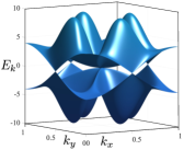
(a) band structure with $\mathcal{C}$

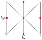
(b) zero modes in (a)

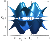
(c) band structure without $\mathcal{C}$

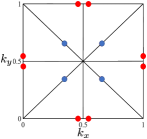
(d) zero modes in (c)

Figure 2: (a) The band of the Hamiltonian $H_{0}$ in (23) with $t=1,\Delta_{2}=1.5$; (b) the blue and red dots illustrate the positions of the zero modes in (a); (c)The Band structure of the Hamiltonian $H_{0}+H_{1}$ with $t=1,\Delta_{2}=1.5,\lambda=0.5,t_{0}=0.6$; (d) the blue and red dots illustrate the positions of the zero modes in (c).

At the $X({1\over 2},0)$ and $Y(0,{1\over 2})$ points, the little co-group $F_{f}^{c}(k)/Z_{2}^{f}=\mathscr{C}_{2v}\times Z_{2}^{\mathcal{C}}\times Z_{2}^{\mathcal{T}}\times Z_{2}^{\mathcal{P}}$ is represented as

$$\!\!\!D(C_{2})=I_{2}\otimes\nu_{z},\ D(\mathcal{M}^{\prime}_{m})=\tau_{z}\otimes\nu_{y},\ D(\mathcal{T}^{\prime})K=I_{4}K,$$

$$\!\!\!D(\mathcal{P})K=\tau_{y}\otimes I_{2}K,\ D(\mathcal{C})=-\mathrm{i}\tau_{y}\otimes\nu_{z},$$

with $m=x,y$ and $\nu_{x,y,z}$ the Pauli matrices acting on the $A,B$ sub-lattices. This rep corresponds to a set of 4-fold irreducible zero modes. Around the $X,Y$ nodal points, the effective $k\cdot p$ Hamiltonian is given by

$$H_{\rm eff}=a\delta k_{1}\tau_{x}\otimes\nu_{y}+b\delta k_{2}\tau_{z}\otimes\nu_{y},$$

where $a,b$ are constants, $k_{1}=k_{y},k_{2}=k_{x}$ for the X point and $k_{1}=k_{x},k_{2}=k_{y}$ for the Y point.

At the $M({1\over 2},{1\over 2})$ point, the little co-group $F_{f}^{c}(M)/Z_{2}^{f}=\mathscr{C}_{4v}\times Z_{2}^{\mathcal{C}}\times Z_{2}^{\mathcal{T}}\times Z_{2}^{\mathcal{P}}$ is represented as

$$D(C^{\prime}_{4})=I_{2}\otimes\nu_{z},\ D(\mathcal{M}^{\prime}_{x})=\tau_{z}\otimes\nu_{y},\ D(\mathcal{T}^{\prime})K=I_{4}K,$$

$$D(\mathcal{P})K=\mathrm{i}\tau_{y}\otimes I_{2}K,\ D(\mathcal{C})=-\mathrm{i}\tau_{y}\otimes\nu_{z}.$$

The dispersion is quadratic at the nodal point $M$ with the following $k\cdot p$ Hamiltonian

$$H_{\rm eff}=a(\delta k_{x}^{2}-\delta k_{y}^{2})\tau_{x}\otimes\nu_{x}+b\delta k_{x}\delta k_{y}\tau_{z}\otimes\nu_{x}.$$

No zero modes appear at the $\Gamma$ point with $F_{f}^{c}(\Gamma)/Z_{2}^{f}=\mathscr{C}_{4v}\times Z_{2}^{\mathcal{C}}\times Z_{2}^{\mathcal{T}}\times Z_{2}^{\mathcal{P}}$. Compared with the M point, $C^{\prime}_{4}$ and $\mathcal{M}^{\prime}_{x}$ are represented differently as $D(C^{\prime}_{4})=I_{2}\otimes I_{2}$ and $D(\mathcal{M}^{\prime}_{x})=\mathrm{i}\tau_{z}\otimes\nu_{x}$, consequently the irrep at $\Gamma$ point correspond to irreducible nonzero modes.

Now we investigate the stability of the zero modes by adding symmetry breaking terms to the Hamiltonian. Interestingly, if one removes the mirror symmetry and preserves all the other symmetries by adding, for instance, the $\Delta_{0}$ perturbation term in Eq.(25), then the dispersion is qualitatively the same as Fig.2(a) and the 4-fold degenerate zero modes at the X, Y and M points still remain. However, unlike the case with $\Delta_{0}=0$ in which all of the 4-fold $\mathcal{C}$-minimal zero modes are irreducible, when $\Delta_{0}\neq 0$ the set of $\mathcal{C}$-minimal zero modes become a direct sum of two sets of 2-fold irreducible zero modes uncoupled to each other.

On the other hand, if one breaks the $\mathcal{C}$ symmetry while preserves all the other symmetries by adding the intra-sublattice terms

$$H_{1}=\lambda\sum_{i,\zeta,\sigma}c^{\dagger}_{i\zeta\sigma}c_{i\zeta\sigma}+t_{0}\sum_{\langle i,j\rangle,\zeta,\sigma}\big{(}c_{i\zeta\sigma}^{\dagger}c_{j\zeta\sigma}+{\rm h.c.}\big{)},$$ (24)

the situations are quite different. From the band structure shown in Figs.2(c)​​ &​​ 2(d) for the parameters $\lambda=0.5,t_{0}=0.6$, one can see that the 4-fold zero modes at the X (or Y) points split into two 2-fold zero modes which are separated along the $\hat{x}$ (or $\hat{y}$) direction. Since the zero modes are away from the high symmetry point, they are now resulting from level crossings protected by different quantum numbers of the $\mathcal{M}^{\prime}_{y}$ (or $\mathcal{M}^{\prime}_{x}$) symmetry. Similarly, the 4-fold zero modes at the M point split into two pairs of 2-fold zero modes, which are separated and spreading along the $(\hat{x}+\hat{y})$- and $(\hat{x}-\hat{y})$- directions respectively. These zero modes are associated with level crossings protected by different quantum numbers of the $\mathcal{M}^{\prime}_{x-y}$ or $\mathcal{M}^{\prime}_{x+y}$ symmetry.

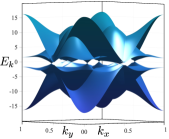
(a) $\mathcal{I}\mathcal{T^{\prime}}$ symmetric: band structure

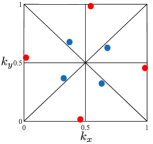
(b) zero modes in (a)

Figure 3: (a) The Band structure of the Hamiltonian $H_{0}+H_{1}+H_{2}$ with $t=1,\Delta_{2}=1.5,\lambda=0.5,t_{0}=0.6,\Delta_{0}=2,\Delta_{1}=1.7$. (b) the blue and red dots illustrate the positions of zero modes in (a).

Zero modes still exist if one breaks both the mirror and $\mathcal{C}$ symmetries by further turning on the nearest neighbor inter-sublattice pairing and intra-sublattice pairing terms

$$H_{2} = \Delta_{0}\!\!\!\sum_{\langle i_{\zeta},j_{\bar{\zeta}}\rangle}\!\!(c_{i_{\zeta}\uparrow}^{\dagger}c_{j_{\bar{\zeta}}\downarrow}^{\dagger}-c_{i_{\zeta}\downarrow}^{\dagger}c_{j_{\bar{\zeta}}\uparrow}^{\dagger})$$ (25)

$$+\Delta_{1}\!\!\sum_{\langle i,j\rangle,\zeta,\sigma}(c_{i\zeta\uparrow}^{\dagger}c^{\dagger}_{j\zeta\downarrow}-c_{i\zeta\downarrow}^{\dagger}c^{\dagger}_{j\zeta\uparrow})+\ {\rm h.c.}$$

Here the $\Delta_{0}$ term breaks the the mirror symmetry while the $\Delta_{1}$ term breaks both the mirror and $\mathcal{C}$ symmetries, and both terms preserve the $C^{\prime}_{4}$ and $\mathcal{T}^{\prime}$ symmetries. The Band structure of the Hamiltonian $H_{0}+H_{1}+H_{2}$ with $t=1,\Delta_{2}=1.5,\lambda=0.5,t_{0}=0.6,\Delta_{0}=2,\Delta_{1}=1.7$ are shown in Fig.3 with the cones protected by the combined $\mathcal{I}\mathcal{T}^{\prime}$ symmetry with $(\widehat{\mathcal{I}\mathcal{T}^{\prime}})^{2}=1$. The $\mathcal{I}\mathcal{T}^{\prime}$ symmetry gives rise to $\pi$-quantized Berry phase for loops in the BZ surrounding a single zero mode, which protects the cones from being solely gapped out. This mechanism makes the zero modes robust when the $\mathcal{I}\mathcal{T}^{\prime}$ symmetry is preserved.

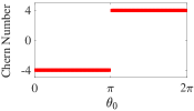
Figure 4: The Chern Number as a function of $\theta_{0}$, with $\theta_{0}$ the phase of $\tilde{\Delta}_{0}=\Delta_{0}e^{\mathrm{i}\theta_{0}}$.

Finally, when the pairing terms are complex, then the time reversal symmetry $\mathcal{T}^{\prime}$ and $\mathcal{I}\mathcal{T}^{\prime}$ are broken and the zero modes disappear. The fully gapped bands becomes a topological SC/SF with nonzero Chern number. Due to the unbroken $C^{\prime}_{4}$ symmetry, the Chern number is either $4$ or $-4$. As shown in Fig.4, if we keep $\Delta_{1,2}$ to be real but vary the phase of $\Delta_{0}$, then the Chern number can be changed from 4 to $-4$ or vice versa. The phase transition occurs at $\theta_{0}={\pi}$ ($\Delta_{0}$ is real again), where the gap closes at 8 nodal points in the BZ.

From the above model, we can see that the zero modes are quit robust even in the presence of symmetry breaking perturbations. When the effective charge conjugation symmetry $\mathcal{C}$ is preserved, the zero modes appear at high symmetry points. When the $\mathcal{C}$ is violated, like in most realist SCs/SFs, the zero modes do not disappear at once as long as certain protecting symmetries are still preserved. The $\mathcal{C}$ symmetry is of theoretical significance in the study of BdG systems in the sense that it provides the physical origin of the zero modes when the $\mathcal{C}$ breaking terms are treated as perturbations. This provides a systematic way to investigate the physical properties of nodal SCs/SFs with gapless quasiparticle excitations.

IV.2 Triangular lattice (spin-${1\over 2}$): $G_{b}=p3\times{Z}_{2}^{\mathcal{T}}$

The second example is a model for $p$-wave SC of the DIII class. We consider the magnetic wallpaper group $G_{b}=p3\times Z_{2}^{\mathcal{T}}$ on triangular lattice, and place two orbitals $[c^{\dagger}_{\uparrow},c^{\dagger}_{\downarrow}]$ at the Wyckoff position $1a(0,0)$ with cite group $\mathscr{C}_{3}\times Z_{2}^{\mathcal{T}}$, as shown in Fig. 5. The bases $[c^{\dagger}_{\uparrow},c^{\dagger}_{\downarrow}]$ respectively carry angular momentum $j=\pm{3\over 2}$ as a consequence of spin-orbit coupling, they reverse their sign under $C_{3}$ and form a Kramers doublet under $\mathcal{T}$.

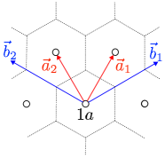
Figure 5: Lattice basis vectors (red) and their dual vectors (blue) for the magnetic wallpaper group $G_{b}=p3\times Z_{2}^{\mathcal{T}}$. The hollow circles label the (maximal) $1a$ Wyckoff positions and the hexagons enclosed by the doted lines stand for unit cells.

In the complete Nambu bases $\Psi^{\dagger}_{i}=[c_{\uparrow}^{\dagger},c_{\downarrow}^{\dagger},c_{\uparrow},c_{\downarrow}]_{i}$, the symmorphic symmetry operations $C_{3}$ and $\mathcal{T}$ are diagonal in the particle-hole sector,

$$\hat{C}_{3}\Psi^{\dagger}_{i}\hat{C}_{3}^{-1}=-\Psi^{\dagger}_{C_{3}i}I_{4},\ \ \hat{\mathcal{T}}\Psi^{\dagger}_{i}\hat{\mathcal{T}}^{-1}=\Psi^{\dagger}_{i}I_{2}\otimes(-\mathrm{i}\sigma_{y})K.$$

With the particle-hole symmetry $\mathcal{P}$ and the effective charge-conjugation symmetry $\mathcal{C}=-e^{-\mathrm{i}{\tilde{\sigma}_{y}\over 2}\pi}e^{-\mathrm{i}{\tilde{\tau}_{y}\over 2}\pi}$ (see (4) and (5)) which act as

$$\ \hat{\mathcal{P}}\Psi^{\dagger}_{i}\hat{\mathcal{P}}^{-1}=[c_{\uparrow},c_{\downarrow},c^{\dagger}_{\uparrow},c^{\dagger}_{\downarrow}]_{i}K,\ \ \widehat{\mathcal{C}}\Psi^{\dagger}_{i}\widehat{\mathcal{C}}^{-1}=[c_{\uparrow},c_{\downarrow},c_{\uparrow}^{\dagger},c_{\downarrow}^{\dagger}]_{i},$$

one obtains the full symmetry group $F^{c}_{f}$. From the band representation, $\mathcal{C}$-minimal zero modes are found at the $\Gamma$ point and the three M points.

To illustrate, we construct the following lattice model preserving the $G_{b}\times Z_{2}^{\mathcal{C}}$ symmetry ($Z_{2}^{\mathcal{C}}=\{E,{\mathcal{C}}\}$),

$$H_{0} = \mathrm{i}t\sum_{\langle ij\rangle}\left(c_{i\uparrow}^{\dagger}c_{j\downarrow}+c_{i\downarrow}^{\dagger}c_{j\uparrow}\right)+\mathrm{i}\Delta_{1}\sum_{\langle ij\rangle}\left(c_{i\uparrow}^{\dagger}c_{j\uparrow}^{\dagger}-c_{i\downarrow}^{\dagger}c_{j\downarrow}^{\dagger}\right)$$ (26)

$$+\mathrm{i}\Delta_{2}\sum_{\langle\langle i^{\prime}j^{\prime}\rangle\rangle}\left(c_{i^{\prime}\uparrow}^{\dagger}c_{j^{\prime}\downarrow}^{\dagger}+c_{i^{\prime}\downarrow}^{\dagger}c_{j^{\prime}\uparrow}^{\dagger}\right)+{\rm h.c.}$$

where the $\langle ij\rangle$ represents the nearest neighbors and $\langle\langle i^{\prime}j^{\prime}\rangle\rangle$ represents the next nearest neighbors. The Hamiltonian can be diagonalized in the full Nambu bases $\Psi^{\dagger}_{k}=[c_{k\uparrow}^{\dagger},c_{k\downarrow}^{\dagger},c_{-k\uparrow},c_{-k\downarrow}]$. The band structure with parameters $t=0.7,\Delta_{1}=0.5,\Delta_{2}=0.4$ is shown in Fig.6, which verifies the existence of zero modes.

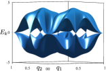
(a) band structure with ${\mathcal{C}}$

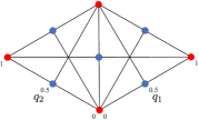
(b) the zero modes in (a)

Figure 6: (a)The Band structure of the Hamiltonian (26); (b) the blue and red dots illustrate the positions of the zero modes.

At the $\Gamma$ point $(0,0)$, the little co-group $F_{f}^{c}(\Gamma)/Z_{2}^{f}=\mathscr{C}_{3}\times Z_{2}^{\mathcal{T}}\times Z_{2}^{\mathcal{P}}\times Z_{2}^{\mathcal{C}}$ is represented as

$$D(C_{3}^{z})=-I_{4},\ \ \ D(\mathcal{T})K=-\mathrm{i}I_{2}\otimes\sigma_{y}K,$$

$$D(\mathcal{P})K=\tau_{x}\otimes I_{2}K,\ D(\mathcal{C})=\tau_{x}\otimes I_{2},$$

in the bases $\Psi^{\dagger}_{k}$. Without $\mathcal{C}$, the little co-group becomes $F_{f}(k)/Z_{2}^{f}=\mathscr{C}_{3}\times Z_{2}^{\mathcal{T}}\times Z_{2}^{\mathcal{P}}$. Defining $\tilde{\mathcal{P}}=\mathcal{T}\mathcal{P}$, then the above rep correspond to a set of minimal nonzero modes of the case (6) in the Tab.1. When $\mathcal{C}$ is turned on, then the rep reduces to two sets of irreducible zero modes which cannot couple to each other. Furthermore, the $k\cdot p$ theory indicates that the lowest order dispersion is cubic (see Sec.III.1), and around the $\Gamma$ point, the third-order $k\cdot p$ Hamiltonian can be written as

$$H_{\rm eff}=h_{1}(\delta k_{x}^{3}-3\delta k_{x}\delta k_{y}^{2})+h_{2}(\delta k_{y}^{3}-3\delta k_{y}\delta k_{x}^{2})$$ (27)

where $k_{x},k_{y}$ are coordinates in the orthogonal frame, and the matrices $h_{1}=(aI_{2}\otimes\nu_{z}+bI_{2}\otimes\nu_{x}+c\tau_{x}\otimes\nu_{z}+d\tau_{x}\otimes\nu_{x}),h_{2}=(a^{\prime}I_{2}\otimes\nu_{z}+b^{\prime}I_{2}\otimes\nu_{x}+c^{\prime}\tau_{x}\otimes\nu_{z}+d^{\prime}\tau_{x}\otimes\nu_{x})$ contain 8 real parameters $a,b,c,d,a^{\prime},b^{\prime},c^{\prime},d^{\prime}$.

At the $C_{3}$ related three $M$ points $(0,{1\over 2}),({1\over 2},0),({1\over 2},{1\over 2})$, the little co-group $F_{f}^{c}(M)/Z_{2}^{f}=Z_{2}^{\mathcal{T}}\times Z_{2}^{\mathcal{P}}\times Z_{2}^{\mathcal{C}}$ is represented as

$$D(\mathcal{T})K=-\mathrm{i}I_{2}\otimes\sigma_{y}K,\ \ D(\mathcal{P})K=\tau_{x}\otimes I_{2}K,$$

$$D(\mathcal{C})=\tau_{x}\otimes I_{2}.$$

For the same reason as the $\Gamma$ point, the $\mathcal{C}$ symmetry turns the minimal nonzero modes into two sets of uncoupled zero modes. The $k\cdot p$ theory indicates that the energy dispersion is linear at the $M$ points (see Sec.III.1), for instance, the $k\cdot p$ Hamiltonian for the $(0,{1\over 2})$ point is given by

$$H_{\rm eff}=h_{1}\delta k_{x}+h_{2}\delta k_{y}$$ (28)

where $h_{1}=(eI_{2}\otimes\nu_{z}+fI_{2}\otimes\nu_{x}+g\tau_{x}\otimes\nu_{z}+h\tau_{x}\otimes\nu_{x}),h_{2}=(e^{\prime}I_{2}\otimes\nu_{z}+f^{\prime}I_{2}\otimes\nu_{x}+g^{\prime}\tau_{x}\otimes\nu_{z}+h^{\prime}\tau_{x}\otimes\nu_{x})$ and $e,f,g,h,e^{\prime},f^{\prime},g^{\prime},h^{\prime}$ are real parameters.

If one breaks the ${\mathcal{C}}$ symmetry (by preserving the time reversal symmetry $\mathcal{T}$) by including the real hopping terms $H_{1}=t_{0}\sum_{\langle i,j\rangle,\sigma}(c_{i\sigma}^{\dagger}c_{j\sigma}+{\rm h.c.})$, or the real pairing terms $H_{2}=\Delta_{0}\sum_{\langle i,j\rangle,\sigma}[(c_{i\uparrow}^{\dagger}c_{j\downarrow}^{\dagger}-c_{i\downarrow}^{\dagger}c_{j\uparrow}^{\dagger})+{\rm h.c.}]$, or the chemical potential term $\lambda\sum_{i\sigma}c_{i\sigma}^{\dagger}c_{i\sigma}$, then the zero modes disappear immediately giving rise to a fully gapped SC/SF state.

IV.3 Triangular lattice (spinless): $G_{b}=p6m\times Z_{2}^{\mathcal{T}}$

The third model is about a SC for spinless fermions of the BDI class. We consider a triangular lattice with the magnetic wallpaper group $G_{b}=p6m\times Z_{2}^{\mathcal{T}}$.

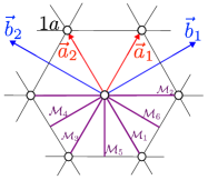
Figure 7: Lattice basis vectors (red) and their dual vectors (blue) for the magnetic wallpaper group $G_{b}=p6m\times Z_{2}^{\mathcal{T}}$. The (maximal) $1a$ Wyckoff positions are indicated by hollow circles, and all mirror plans are indicated by purple lines.

We put spinless fermonic bases $[c^{\dagger},c]$ on the Wyckoff position $1a(0,0)$ which carry projective rep of the site group $C_{3v}\times\mathscr{C}_{\mathcal{I}}\times Z_{2}^{\mathcal{T}}$, see Fig.7. In the fermionic symmetry group $G_{f}$, the inversion operation $\mathcal{I}$ is associated with a charge operation, namely $\mathcal{I}^{\prime}=(e^{\mathrm{i}{{\tau}_{z}\over 2}\pi}||\mathcal{I})$. The Nambu bases $\Psi^{\dagger}_{i}=[c^{\dagger},c]_{i}$ vary under the action of the symmetry group as

$$\hat{C}_{3}\Psi^{\dagger}_{i}\hat{C}_{3}^{-1}=\Psi^{\dagger}_{C_{3}i},\ \ \hat{\mathcal{M}}_{m}\Psi^{\dagger}_{i}\hat{\mathcal{M}}_{m}^{-1}=\Psi^{\dagger}_{\mathcal{M}_{m}i},$$

$$\hat{\mathcal{I}}^{\prime}\Psi^{\dagger}_{i}\hat{\mathcal{I}}^{{}^{\prime}-1}=\Psi^{\dagger}_{\mathcal{I}i}(\mathrm{i}{\tau}_{z})=[\mathrm{i}c^{\dagger},-\mathrm{i}c]_{\mathcal{I}i},\ \ \mathcal{T}\Psi^{\dagger}_{i}\mathcal{T}^{-1}=\Psi^{\dagger}_{i},$$

with $m=4,5,6$. Besides the particle-hole operation $\mathcal{P}\Psi^{\dagger}_{i}\mathcal{P}^{-1}=\Psi^{\dagger}_{i}{\tau}_{x}K=[c,c^{\dagger}]_{i}K$, we further consider the following charge conjugation $\mathcal{C}$ with

$$\hat{\mathcal{C}}\Psi^{\dagger}_{i}\hat{\mathcal{C}}^{-1}=\Psi^{\dagger}_{i}{\tau}_{y}=[\mathrm{i}c,-\mathrm{i}c^{\dagger}]_{i}.$$

The band representation of the above group $F^{c}_{f}$ indicates that the high symmetry lines on the mirror planes $\mathcal{M}_{1,2,3}$ (i.e. the lines linking $\Gamma$ and $K,K^{\prime}$ points) are nodal lines with 2-fold zero modes.

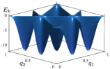
(a) band structure with $\mathcal{C}$ symmetry

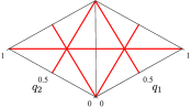
(b) the nodal lines in (a)

Figure 8: The nodal-line Band structure of the Hamiltonian (29) having $\mathcal{C}$ symmetry.

The simplest lattice model preserving the above symmetry is a pure pairing model,

$$H_{0}=\Delta\sum_{\langle\langle ij\rangle\rangle}c_{i}^{\dagger}c_{j}^{\dagger}+{\rm h.c.}$$ (29)

where $\langle\langle ij\rangle\rangle$ represents next nearest neighbors (the nearest neighbor pairing terms break the $\mathcal{M}_{4,5,6}$ symmetries).

The band structure with parameter $\Delta=2$ is shown in Fig.8, where the three nodal liens (locating on the mirror planes $\mathcal{M}_{1,2,3}$) have the symmetry group $F_{f}^{c}(k)/Z_{2}^{f}=Z_{2}^{\mathcal{C}}\times Z_{2}^{\mathcal{I}^{\prime}\mathcal{T}}\times Z_{2}^{\mathcal{M}\mathcal{T}}\times Z_{2}^{\mathcal{T}\mathcal{P}}$. The symmetry group $F_{f}^{c}(k)$ is represented as

$$D(\mathcal{I}^{\prime}\mathcal{T})K=\mathrm{i}{\tau}_{z}K,\ D(\mathcal{T}\mathcal{P})={\tau}_{x},$$

$$D(\mathcal{C})={\tau}_{y},\ D(\mathcal{M}_{m}\mathcal{T})K=I_{2}K,{\ m=4,5,6}.$$

It can be seen that the subgroup $Z_{2}^{\mathcal{C}}\times Z_{2}^{\mathcal{M}\mathcal{T}}\times Z_{2}^{\mathcal{P}}$ can protect the nodal lines. The $k\cdot p$ Hamiltonian at the nodal lines are given as

$$H_{\rm eff3}=a\delta k_{v}{\tau}_{y},\ \ H_{\rm eff2}=-a\delta k_{x}{\tau}_{y},\ \ H_{\rm eff1}=a\delta k_{w}{\tau}_{y}.$$

where $k_{x},k_{y}$ are coordinates in the orthogonal frame and $\delta k_{v}={1\over 2}\delta k_{x}+{\sqrt{3}\over 2}\delta k_{y},\delta k_{w}={1\over 2}\delta k_{x}-{\sqrt{3}\over 2}\delta k_{y}$.

Now we break the $\mathcal{C}$ symmetry by adding the terms

$$H_{1}=\lambda\sum_{i}c_{i}^{\dagger}c_{i}+\big{(}t\sum_{\langle i,j\rangle}c_{i}^{\dagger}c_{j}+{\rm h.c.}\big{)},$$

then the zero modes on the nodal line are lifted except for six nodal points, as shown in Figs.9(a) ​​& ​​9(b). These nodal points are resulting from level crossing protected by the quantum numbers of the mirror symmetries $\mathcal{M}^{\prime}_{1,2,3}=\mathcal{I}^{\prime}\mathcal{M}_{4,5,6}$, and the six nodal points are related with each other by $C_{3}$ and $\mathcal{I}^{\prime}$ symmetries. The $k\cdot p$ effective Hamiltonian for the three nodal points are

$$H^{\prime}_{\rm eff3}=a\delta k_{v}{\tau}_{y}+b\delta k_{\tilde{v}}{\tau}_{z},\ \ H^{\prime}_{\rm eff2}=-a\delta k_{x}{\tau}_{y}-b\delta k_{y}{\tau}_{z},$$

$$H^{\prime}_{\rm eff1}=a\delta k_{w}{\tau}_{y}+b\delta k_{\tilde{w}}{\tau}_{z},$$

with $\delta k_{v}={1\over 2}\delta k_{x}+{\sqrt{3}\over 2}\delta k_{y},\delta k_{\tilde{v}}=-{\sqrt{3}\over 2}\delta k_{x}+{1\over 2}\delta k_{y},\delta k_{w}={1\over 2}\delta k_{x}-{\sqrt{3}\over 2}\delta k_{y},\delta k_{\tilde{w}}={\sqrt{3}\over 2}\delta k_{x}+{1\over 2}\delta k_{y}$.

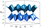
(a) band structure with $\mathcal{M}^{\prime}_{1,2,3}$

(b) zero modes inf (a)

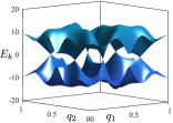
(c) band structure without $\mathcal{M}^{\prime}_{1,2,3}$

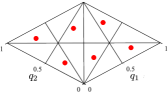
(d) zero modes in (c)

Figure 9: (a)Band structure of the Hamiltonian (29) with parameters $t=1.5,\lambda=0.1,\Delta=2$. The mirror symmetries $\mathcal{M}^{\prime}_{1,2,3}$ are preserved; (b) the red dots illustrate the positions of the zero modes in (a); (c) Band structure for $t=1.5,\lambda=0.1,\Delta=2,\Delta_{2}=-2.5$. The mirror symmetries are violated but the $\mathcal{I^{\prime}T}$ symmetry is preserved; (d) the red dots illustrate the positions of the zero modes in (c).

If we further break the mirror symmetry $\mathcal{M}^{\prime}_{1,2,3}$ by adding the nearest pairing term

$$H_{2}=\Delta_{2}\sum_{\langle i,j\rangle}c_{i}^{\dagger}c_{j}^{\dagger}+{\rm h.c.},$$ (30)

the nodal points still exist but their positions drift away the high symmetry lines, as shown in Figs.9(c)​​ &​​ 9(d). These nodal points are protected by the $\mathcal{I}^{\prime}\mathcal{T}$ symmetry with $(\widehat{\mathcal{I}^{\prime}\mathcal{T}})^{2}=1$. If we break the time-reversal symmetry by setting $\Delta_{2}$ as a complex number, then all the zero modes are removed and a topological SC/SF is obtained with Chern number $\pm 3$.

IV.4 Multi-node $Z_{2}$ QSL on Honeycomb lattice: $G_{b}=p\bar{3}1m\times Z_{2}^{\mathcal{T}}$

The fourth example is a $Z_{2}$ spin liquid model whose symmetry group is a PSG containing ‘off-diagonal’ elements in the particle-hole sector. We adopt the PSG of the exactly solvable Kitaev spin liquid on the honeycomb lattice Kitaev [2006], You et al. [2012] whose magnetic layer group is $G_{b}=p\bar{3}1m\times Z_{2}^{\mathcal{T}}$ with point group $D_{3d}\times Z_{2}^{\mathcal{T}}$, see Fig.10. Placing spin-${1\over 2}$ Nambu bases $\Psi^{\dagger}_{i,\zeta}\equiv[c^{\dagger}_{\uparrow},c^{\dagger}_{\downarrow},c_{\uparrow},c_{\downarrow}]_{i,\zeta},\ \zeta=A,B$ respectively at the $2c$ Wyckoff positions $A=({1\over 3},{2\over 3})$ and $B=({2\over 3},{1\over 3})$ of the $i$th unit cell, then the PSG is obtained by replacing the generators $C_{3c},C_{2{\alpha}},\mathcal{T},\mathcal{I}$ of $D_{3d}\times Z_{2}^{T}$ by the spin and charge dressed operations (see (4) and (5))

$$C_{3c}^{\prime}\!=\!(e^{-\mathrm{i}{\tilde{\tau}_{c}\over 2}{2\pi\over 3}}e^{-\mathrm{i}{\tilde{\sigma}_{c}\over 2}{2\pi\over 3}}||C_{3c}),\ C_{2{\alpha}}^{\prime}\!=\!(e^{-\mathrm{i}{\tilde{\tau}_{{\alpha}}\over 2}{\pi}}e^{-\mathrm{i}{\tilde{\sigma}_{{\alpha}}\over 2}{\pi}}||C_{2{\alpha}}),$$

$$\mathcal{T}^{\prime}=(P_{f}^{B}e^{-\mathrm{i}{\tau_{y}\over 2}{\pi}}e^{-\mathrm{i}{\sigma_{y}\over 2}{\pi}}K||\mathcal{T}),\ \mathcal{I}^{\prime}=(P_{f}^{B}||\mathcal{I}),$$

where $\tilde{\tau}_{c}={1\over\sqrt{3}}(\tilde{\tau}_{x}+\tilde{\tau}_{y}+\tilde{\tau}_{z}),\tilde{\tau}_{{\alpha}}={1\over\sqrt{2}}(\tilde{\tau}_{y}-\tilde{\tau}_{z})$ and $\tilde{\sigma}_{c},\tilde{\sigma}_{{\alpha}}$ are similarly defined. The Nambu bases $[\Psi^{\dagger}_{i,A},\Psi^{\dagger}_{i,B}]$ carry a 8-D projective rep of the site group $D_{3}\times Z_{2}^{\mathcal{T}}$ with

$$\hat{\mathcal{T}}^{\prime}[\Psi^{\dagger}_{i,A},\Psi^{\dagger}_{i,B}]\hat{\mathcal{T}^{\prime}}^{-1}=[\Psi^{\dagger}_{i,A},\Psi^{\dagger}_{i,B}]\nu_{z}\otimes{\tau}_{x}\otimes I_{2}K,$$

$$\hat{\mathcal{I}}^{\prime}[\Psi^{\dagger}_{i,A},\Psi^{\dagger}_{i,B}]\hat{\mathcal{I}}^{{}^{\prime}-1}=[\Psi^{\dagger}_{\mathcal{I}(i),B},-\Psi^{\dagger}_{\mathcal{I}(i),A}],$$

and

$$\hat{C}_{3c}^{\prime}\Psi^{\dagger}_{i,\zeta}\hat{C_{3c}^{\prime}}^{-1}={1\over 2}\Psi^{\dagger}_{C_{3c}(\mathrm{i}),\zeta}\left(\begin{matrix}1&{-\mathrm{i}}&1&{-\mathrm{i}}\\ 1&{\mathrm{i}}&{-1}&{-\mathrm{i}}\\ 1&{\mathrm{i}}&1&{\mathrm{i}}\\ {-1}&{\mathrm{i}}&1&{-\mathrm{i}}\end{matrix}\right),$$

$$\hat{C}_{2{\alpha}}^{\prime}\Psi^{\dagger}_{i,\zeta}\hat{C_{2{\alpha}}^{\prime}}^{\!\!-1}={1\over 2}\Psi^{\dagger}_{C_{2{\alpha}}(i),\zeta}\left(\begin{matrix}{-1}&{-\mathrm{i}}&{-1}&{-\mathrm{i}}\\ {\mathrm{i}}&{1}&{-\mathrm{i}}&{-1}\\ {-1}&{\mathrm{i}}&{-1}&{\mathrm{i}}\\ {\mathrm{i}}&{-1}&{-\mathrm{i}}&{1}\end{matrix}\right).$$

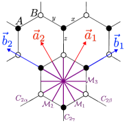
Figure 10: Lattice basis vectors (red) and their dual vectors (blue) for the magnetic layer group $G_{b}=p\bar{3}1m\times Z_{2}^{\mathcal{T}}$. The (maximal) $2c$ Wyckoff positions $A,B$ are indicated by black dots and hollow circles respectively, and all mirror plans and 2-fold axes are indicated by purple lines.

Considering nearest and next next nearest neighbor terms between different sub-lattices, the most general BdG Hamiltonian that preserves the above PSG is given by (the intra-sub-lattice terms are not allowed by the PSG)

$$\!\!\!H_{0} \!\!\!=\!\!\!\! \sum_{\langle i,j\rangle\in z}\!\!\big{(}\Psi_{i,A}^{\dagger}U\mathcal{H}_{1}U^{\dagger}\Psi_{j,B}\!+{\rm h.c.}\big{)}+(\mbox{x-,y-bonds})+$$ (31)

$$\!\!\!\!\!\sum_{\langle\langle\langle i,j^{\prime}\rangle\rangle\rangle\in Z}\!\!\!\!\!\!\big{(}\Psi_{i,A}^{\dagger}U\mathcal{H}_{2}U^{\dagger}\Psi_{j^{\prime},B}\!+\!{\rm h.c.}\big{)}\!\!+\!(\mbox{X-,Y-bonds}),$$

where $\mathcal{H}_{1},\mathcal{H}_{2}$ are the Hamiltonian matrices in the Majorana bases

$$\mathcal{H}_{1}=\mathrm{i}\left(\begin{matrix}\!\!\eta_{0}&\eta_{1}&-\eta_{1}&0\\ \!\!\eta_{1}&\eta_{2}&\eta_{4}&\eta_{3}\\ \!\!-\eta_{1}&\eta_{4}&\eta_{2}&\eta_{3}\\ \!\!0&\eta_{3}&\eta_{3}&\eta_{5}\end{matrix}\right)\!,\mathcal{H}_{2}=\mathrm{i}\left(\begin{matrix}\!\!\eta^{\prime}_{0}&\eta^{\prime}_{1}&-\eta^{\prime}_{1}&0\\ \!\!\eta^{\prime}_{1}&\eta^{\prime}_{2}&\eta^{\prime}_{4}&\eta^{\prime}_{3}\\ \!\!-\eta^{\prime}_{1}&\eta^{\prime}_{4}&\eta^{\prime}_{2}&\eta^{\prime}_{3}\\ \!\!0&\eta^{\prime}_{3}&\eta^{\prime}_{3}&\eta^{\prime}_{5}\end{matrix}\right)\!,$$

and $U\!\!=\!\!{1\over\sqrt{2}}\left(\begin{matrix}1&0&0&{\mathrm{i}}\\ 0&{\mathrm{i}}&{-1}&0\\ {1}&0&0&{-\mathrm{i}}\\ 0&{-\mathrm{i}}&{-1}&0\end{matrix}\right)$ is the transformation matrix mapping the complex fermion bases $\Psi^{\dagger}_{i,\zeta}$ into the Majorana basesKitaev [2006], namely $[c,b_{x},b_{y},b_{z}]_{i,\zeta}=\Psi^{\dagger}_{i,\zeta}U$. The parameters $\eta_{0,1,2,3,4,5}$, $\eta^{\prime}_{0,1,2,3,4,5}$ are real numbers among which $\eta_{0},\eta_{5}$ come from the solution of the pure Kitaev model. The terms on the x-,y-bonds (X-,Y-bonds) can be obtained from ones on the z-bonds (Z-bonds) by successive $C^{\prime}_{3c}$ rotations.

The spectrum of the Hamiltonian (31) can support a series of zero modes in the BZ and the corresponding state is a multi-node QSL. For instance, Fig.11 shows the band structure with parameters $\eta_{0}=2,\eta_{1}=1.2,\eta_{2}=0.8,\eta_{3}=0.5,\eta_{4}=0.2,\eta_{5}=1.2$ and $\eta^{\prime}_{0}=1.6,\eta^{\prime}_{1}=0.2,\eta^{\prime}_{2}=0.8,\eta^{\prime}_{3}=2.5,\eta^{\prime}_{4}=0,\eta^{\prime}_{5}=0$. There are totally $20$ cones, where the $2$ cones in green color are irreducible zero modes protected by the little co-group $F_{f}(K)=\mathscr{C}^{\prime}_{3v}\times Z_{2}^{\mathcal{I}^{\prime}\mathcal{T}^{\prime}}$; the $6$ cones in blue color are protected by crossing of energy bands carrying different quantum numbers of the mirror symmetries $\mathcal{M}^{\prime}_{1,2,3}$; the $12$ cones in red color are protected by $\pi$-quantized Berry phase due to the $\mathcal{I^{\prime}T^{\prime}}$ symmetry.

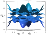
(a) Kitaev QSL: band structure

(b) Kitaev QSL: positions of the zero modes

Figure 11: (a)The Band structure of the Hamiltonian (31) with parameters given in the maintext. The number of the cones is ‘$12+6+2$’ where the ‘$12$’ is protected by the effective $\mathcal{I^{\prime}T^{\prime}}$ symmetry, the ‘$6$’ is protected by the effective mirror reflection symmetries $\mathcal{M}^{\prime}_{1,2,3}$, and the ‘$2$’ form a set of irreducible zero modes; (b) the dots illustrate the positions of the zero modes in (a).

The two high symmetry points $K=({1\over 3},{2\over 3})$ and $K^{\prime}=({2\over 3},{1\over 3})$ have the little co-group $F_{f}(k)/Z_{2}^{f}=\mathscr{C}^{\prime}_{3v}\times Z_{2}^{\mathcal{I^{\prime}T^{\prime}}}\times Z_{2}^{\mathcal{PT^{\prime}}}$. All of the $C^{\prime}_{3c}$, $\mathcal{M^{\prime}}_{1,2,3}$, $\mathcal{I}^{\prime}\mathcal{T}^{\prime}$ symmetries can be treated as effective charge conjugation, and the two fold irreducible zero modes are represented as

$$D(C^{\prime}_{3c})={\sqrt{3}\over 2}I+{\mathrm{i}\over 2}\mu_{z},\ \ D(\mathcal{M}^{\prime}_{1})={\sqrt{3}\mathrm{i}\over 2}\mu_{y}-{\mathrm{i}\over 2}\mu_{x},$$

$$D(\mathcal{I^{\prime}T^{\prime}})=\mu_{x}K,\ \ D(\mathcal{T^{\prime}P})=-\mu_{z}.$$

According to Eq.(III.1) one has $a_{({\rm v\times ph})}=1$. So the dispersion around the $K$ and $K^{\prime}$ points is linear and the $k\cdot p$ Hamiltonian has one free parameter $v$, yielding

$$H_{\rm eff1}=v(\delta k_{x}\mu_{x}+\delta k_{y}\mu_{y}).$$

Similarly, the $k\cdot p$ Hamiltonian for the cones at the high symmetry lines with mirror symmetries $\mathcal{M}^{\prime}_{1,2,3}$ have two free parameters $u,v$. For example, around the left blue cone, the effective Hamiltonian reads

$$H_{\rm eff2}= u\delta k_{x}{\sqrt{2}\over 2}(\cos\theta_{2}\mu_{x}-\sin\theta_{2}\mu_{y})$$

$$+v\delta k_{y}{\sqrt{2}\over 2}(\sin\theta_{2}\mu_{x}+\cos\theta_{2}\mu_{y})$$

with $\theta_{2}\approx 0.47\pi$. Furthermore, the $k\cdot p$ Hamiltonian for the cones at a generic point is given as

$$H_{\rm eff}=(e\mu_{x}+f\mu_{y})\delta k_{x}+(h\mu_{x}+m\mu_{y})\delta k_{y},$$ (32)

which has four parameters $e,f,h,m$.

Notice that the point group symmetry elements are associated with charge and spin operations in the PSG. This makes the symmetries easy to break. For instance, the Zeeman coupling term $H_{1}=B\sum_{i,\zeta}\Psi_{i,\zeta}^{\dagger}{\tilde{\sigma}_{c}\over 2}\Psi_{i,\zeta}$ from a weak magnetic field breaks the symmetries $e^{-\mathrm{i}{\tilde{\sigma}_{\alpha}\over 2}\pi},e^{-\mathrm{i}{\tilde{\sigma}_{y}\over 2}\pi}K$ in the spin sector. Consequently the mirror symmetries $\mathcal{M}^{\prime}_{1,2,3}$ and the time reversal symmetry $\mathcal{T}^{\prime}$ in the PSG are broken, hence all of the cones are gapped out. The resulting state has nonzero Chern number $\pm 8$. Furthermore, a chemical potential term $H_{2}={\lambda}\sum_{i,\zeta}(\Psi^{\dagger}_{i,\zeta}{\tilde{\tau}_{z}\over 2}\Psi_{i,\zeta})+{\rm const}$ can be introduced by doping the system with charge carriers. This term breaks the $e^{-\mathrm{i}{\tilde{\tau}_{\alpha}\over 2}\pi},e^{-\mathrm{i}{\tilde{\tau}_{y}\over 2}\pi}K$ symmetries in the charge sector, consequently the mirror symmetries $\mathcal{M}^{\prime}_{1,2,3}$ and the time reversal symmetry $\mathcal{T}^{\prime}$ in the PSG are also broken. All of the cones are then gapped out, resulting in a topological SC state with nonzero Chern number $\pm 2$You et al. [2012], Zhang and Liu [2021] (SC with hole doping has opposite Chern number with the one with electron doping).

In Fig.11, the cones with the same color are symmetry related and form a $\{k^{*}\}$. With the varying of the parameters $\eta_{0}\sim\eta_{5}$ and $\eta^{\prime}_{0}\sim\eta^{\prime}_{5}$, the positions of the cones, the number of the cones and even the pattern of the cones (the collection of several $\{k^{*}\}$) may change accordingly. The pattern of the cones determines the physical response of probe fields. Hence spin liquid states with the same pattern of cones can be considered as belonging to the same phase. Therefore, the pattern of cones is an important information of a gapless QSL in addition to the PSG.

V Discussion and Conclusion

Before concluding this work, we comment on some interesting issues.

To be Majorana or not. We have shown that with the protection of effective charge conjugation symmetry $\mathcal{C}$, zero modes can appear at high symmetry points. Since the charge conjugation transform a particle into its anti-particle, the quasiparticle corresponding to the $\mathcal{C}$-protected zero modes is its own anti-particle and can be identified as a Majorana quasiparticle.

We have also shown that when the effective charge conjugation symmetry $\mathcal{C}$ is violated, bulk zero modes can also appear due to quantum numbers protected level crossing or $\mathcal{I}^{\prime}\mathcal{T}^{\prime}$ protected quantized Berry phase. Since the Hamiltonian is not commuting with $\mathcal{C}$, so the $\mathcal{C}$ transformed quasiparticle is not an eigenstate of the Hamiltonian. Therefore, strictly speaking, the zero modes without $\mathcal{C}$ symmetry is not a Majorana quasiparticle.

Although $\mathcal{P}$ is always anti-commuting with the Hamiltonian, $\mathcal{P}$ transformed quasiparticles are not independent on the original quasiparticles since $\mathcal{P}$ is an redundancy of the SCs/SFs/QSLs.

Classification of nodal SCs/SFs/QSLs. If two BdG systems have the same symmetry, and their low-energy quasiparticles are one-to-one corresponding to each other, then we can identify the two systems as a same phase. In this sense, we can provide a method to classify gapless nodal SCs/SFs/QSLs:

(i) the symmetry group, which is an extension of the space group of the lattice by internal symmetries such as spin rotation and charge operations. A systematic study of all allowed symmetry groups for given lattice structure will be given elsewhereendnote72.

(ii) the pattern of the bulk zero modes, whose positions form several sets of $k$ stars, namely $\{k^{\star}\}$, where each $k^{\star}$ is a set of symmetry related equivalent momentum points. For the set of $\{k^{\star}\}$, we also know the total number of zero energy nodes of the system.

(iii) the degeneracy of the zero modes in every point of $\{k^{\star}\}$. The degeneracy of zero modes at equivalent $k$ points are the same.

(iv) the dispersion and physical properties of the quasiparticles, which are described by the $k\cdot p$ effective theory.

Effect of interactions. It can be expected that under weak interactions, the quasiparticles corresponding to the bulk zero modes remain gapless. However, with the increasing of the interaction strength, the fate of the quasiparticles is dependent on the degeneracy as well as the form of dispersion. Quantitative results should be obtained using renormalization group calculations, and will not be discussed here.

In summary, using the theory of projective reps, we systematically studied the symmetry conditions of bulk zero modes in the mean field theory of superconductors, superfluids and $Z_{2}$ QSLs where fermions pair to form Cooper pairs. We than provided an efficient method to obtain the $k\cdot p$ effective theory of these gapless quasiparticles, from which one can get the dispersions as well as their physical response to external fields. The positions of the zero modes can be controlled by adjusting the symmetry of the Hamiltonian. Furthermore, the dispersion of the gapless quasiparticles can be linear or of higher order. The above results are illustrated via concrete lattice modes. Our symmetry representation-based theory is complementary to the topological origin (theory of symmetry indicators) of gapless quasiparticles in BdG systems, and is helpful for experimental realization of Majorana like gapless quasiparticles.

We thank Yu-Xin Zhao, Zhi-Da Song, Chen Fang, Yuan-Ming Lu, Jiucai Wang and Bruce Normand for helpful discussions. A.Z.Y thank Xiao-Yue Wang for her helpful comments. This work is supported by NSFC (Grants No.12374166, 12134020) and National Basic Research and Development plan of China (Grants No.2023YFA1406500, 2022YFA1405300).

Appendix A Meaning of Pauli matrices $\boldsymbol{\tau},\boldsymbol{\sigma},\boldsymbol{\mu},\boldsymbol{\nu},\boldsymbol{\omega}$

In the main text, we have used different notations of Pauli matrices. In the following we list their physical meaning.

$\tau_{x,y,z}$ generate the charge $SU(2)$ group and act on the particle-hole degrees of freedom. For instance the charge conjugation can be chosen as $\mathcal{C}=e^{-i{\tau_{x}\over 2}\pi}$. The product of $\tau_{x,y,z}$ with identity matrix are noted as $\Gamma_{x,y,z}=\tau_{x,y,z}\otimes I$.

$\sigma_{x,y,z}$ generate the spin $SU(2)$ group and act on the spin degrees of freedom.

$\mu_{x,y,z}$ act on the positive/negative eigen spaces of the Hamiltonian. The eigenvalue $1$ (or $-1$) of $\mu_{z}$ labels the positive (or negative) eigen sapce of the total Hamiltonian, and $\mu_{x,y}$ exchange the two subspaces.

$\nu_{x,y,z}$ act on the A,B sublattices. The eigenvalue $1$ (or $-1$) of $\nu_{z}$ labels the positive (or negative) labels the A (or B) sublattice, and $\nu_{x,y}$ exchange the two sublattices.

For an irrep $D(G)$ of anti-unitary group $G$ of the $\mathbb{C}$ or $\mathbb{H}$ type, one can reduce the restricted rep $D(H)$ into two irreps with $H$ the maximal unitary subgroup of $G$. $\omega_{x,y,z}$ acts on the irrep spaces of $D(H)$. The eigenvalue $\pm 1$ of $\omega_{z}$ respectively labels the two irrep spaces, and $\omega_{x,y}$ exchange the two subspaces.

Appendix B Proof of $[D(\mathcal{P})K,D(g)K_{s(g)}]=0$

In the Nambu bases $\Psi^{\dagger}=[c_{1}^{\dagger},...,c_{N}^{\dagger},c_{1},...,c_{N}]$, suppose a general symmetry operation $g$ (mixing or non-mixing) is represented as

$$\hat{g}\Psi^{\dagger}\hat{g}^{-1}=\Psi^{\dagger}\begin{pmatrix}A(g)&B^{*}(g)\\ B(g)&A^{*}(g)\end{pmatrix}K_{s(g)}=\Psi^{\dagger}D(g)K_{s(g)}.$$

Specially, the particle-hole symmetry is represented as $D(\mathcal{P})K=[\tau_{x}\otimes I_{N}]K=\Gamma_{x}K$. Due to the fact that $D(g)=[I_{2}\otimes\rm{Re}(A)+\mathrm{i}\tau_{z}\otimes\rm{Im}(A)+\tau_{x}\otimes\rm{Re}(B)+\tau_{y}\otimes\rm{Im}(B)]$ and that $\tau_{x}K$ commutes with the four matrices $\{I_{2},\mathrm{i}\tau_{z},\tau_{x},\tau_{y}\}$, it is easily verified that $D(g)\Gamma_{x}=\Gamma_{x}[D(g)]^{*},$ Namely,

$$D(g)K_{s(g)}D(\mathcal{P})K=D(\mathcal{P})KD(g)K_{s(g)}.$$

This conclusion can be seen more straightforwardly in the majorana representation with

$$\gamma_{i}^{l}=c_{i}+c_{i}^{\dagger},\ \ \gamma_{i}^{r}=-i(c_{i}-c_{i}^{\dagger}),$$

$$\{\gamma_{i}^{\alpha},\gamma_{j}^{\beta}\}=2\delta_{\alpha\beta}\delta_{ij},\ \ \alpha,\beta=l,r.$$

With these bases, any symmetry operation $g$ is represented as a REAL matrix $\mathscr{D}(g)$, especially $\mathcal{P}$ is represented as $\mathscr{D}(\mathcal{P})=I_{2N}K$. Hence the commutation of $\mathscr{D}(\mathcal{P})K$ and the real rep $\mathscr{D}(g)K_{s(g)}$ manifests itself.

In the reduced Nambu subspaces $\psi^{\dagger}=[C_{\uparrow}^{\dagger},C_{\downarrow}^{T}]$ with $C_{\uparrow}^{\dagger}=[c_{1\uparrow}^{\dagger},c_{2\uparrow}^{\dagger},...,c_{L\uparrow}^{\dagger}]$, $C_{\downarrow}^{T}=[c_{1\downarrow},c_{2\downarrow},...,c_{L\downarrow}]$ for spin-${1\over 2}$ fermions having spin rotation symmetry, one has $\mathcal{P}^{2}=-1$ with $D(\mathcal{P})K=\mathrm{i}\tau_{y}\otimes I_{L}K$. Generally, a symmetry operation $g$ acts on the lattice and charge (but no spin) degrees of freedom as

$$\hat{g}\psi^{\dagger}\hat{g}^{-1}\!=\!\psi^{\dagger}\!\begin{pmatrix}A(g)&-B^{*}(g)\\ B(g)&A^{*}(g)\end{pmatrix}\!\!K_{s(g)}\!=\!\psi^{\dagger}D(g)K_{s(g)},$$ (33)

which can be decomposed as $D(g)=[I_{2}\otimes\rm{Re}(A)+\mathrm{i}\tau_{z}\otimes\rm{Im}(A)+\mathrm{i}\tau_{x}\otimes\rm{Im}(B)-\mathrm{i}\tau_{y}\otimes\rm{Re}(B)].$ Since $\mathrm{i}\tau_{y}K$ commutes with the four matrices $\{I_{2},\mathrm{i}\tau_{z},\mathrm{i}\tau_{x},\mathrm{i}\tau_{y}\}$. So, $[D(\mathcal{P})K,D(g)K_{s(g)}]=0$.

Now we verify the equation (33). Suppose $g$ acts on $C_{\uparrow}^{\dagger}$ as

$$\hat{g}C_{\uparrow}^{\dagger}\hat{g}^{-1}=\left(C_{\uparrow}^{\dagger}A(g)+C_{\downarrow}^{T}B(g)\right)K_{s(g)}.$$

Noticing that $C_{\uparrow}^{\dagger}$ and $C_{\downarrow}^{T}$ are related by complex conjugation, we have $\hat{g}C_{\uparrow}^{T}\hat{g}^{-1}=\left(C_{\uparrow}^{T}A^{*}(g)+C_{\downarrow}^{\dagger}B^{*}(g)\right)K_{s(g)}.$ On the other hand, noticing that $\hat{C}_{2y}C_{\uparrow}^{T}\hat{C}_{2y}^{-1}=C_{\downarrow}^{T},\hat{C}_{2y}C_{\downarrow}^{\dagger}\hat{C}_{2y}^{-1}=-C_{\uparrow}^{\dagger}$ and that $\hat{C}_{2y}$ commutes with $\hat{g}$ (because $\hat{C}_{2y}$ only acts on spin while $\hat{g}$ does not act on spin), therefore

$$\hat{g}C_{\downarrow}^{T}\hat{g}^{-1} = \hat{g}\hat{C}_{2y}C_{\uparrow}^{T}\hat{C}_{2y}^{-1}\hat{g}^{-1}=\hat{C}_{2y}\hat{g}C_{\uparrow}^{T}\hat{g}^{-1}\hat{C}_{2y}^{-1}$$

$$= \left(\hat{C}_{2y}C_{\uparrow}^{T}\hat{C}_{2y}^{-1}A^{*}(g)+\hat{C}_{2y}C_{\downarrow}^{\dagger}\hat{C}_{2y}^{-1}B^{*}(g)\right)K_{s(g)}$$

$$= \left(-C_{\uparrow}^{\dagger}B^{*}(g)+C_{\downarrow}^{T}A^{*}(g)K_{s(g)}\right)K_{s(g)},$$

which yields eq.(33).

Appendix C Generalized band representation for SCs/SFs/QSLs

When the pairing terms are switched off, the SCs/SFs become metals or insulators where a number of localized orbitals in the unit cell in real space determine the energy band structure in the Brillouin zone. The energy bands as entire entities form a special representation of the system’s symmetry group $G$ called the band representation Zak [1982], Bradlyn et al. [2017b], Cano and Bradlyn [2021]. Such a band rep is called elementary if it cannot be decomposed as a direct sum of smaller band representations. Once the elementary band reps are known, all the band reps can be obtained by the direct sum of elementary ones.

The band representations can be generalized to BdG systems by introducing ‘particle-hole’ degrees of freedom. We start from the full ‘symmetry’ group $F_{f}=G_{f}+\mathcal{P}G_{f}$. The construction of an elementary band representation needs two ingredients. The first is a ‘maximal’ Wyckoff position $q_{1}$ with a site-symmetry group $G_{q_{1}}$ (composed of operations in $G_{f}$ which stabilize the site $q_{1}$). The second is a set of creation and annihilation operators of localized orbitals $\phi_{1}(q-q_{1}-R_{m}),\phi_{2}(q-q_{1}-R_{m}),...,\phi_{r}(q-q_{1}-R_{m})$ centered at $q_{1}$ in the $m$-th unit cell, namely $[c_{\sigma,q_{1}+R_{m}}^{\dagger},c_{\sigma,q_{1}+R_{m}}]$ with $\sigma=1,2,...,r$ and

$$c_{\sigma,q_{1}+R_{m}}^{\dagger}|{\rm vac}\rangle\equiv\phi_{\sigma}(q-q_{1}-R_{m}),$$

where $|{\rm vac}\rangle$ is the vacuum state.

The operators $[c_{\sigma,q_{1}}^{\dagger},c_{\sigma,q_{1}}]$ carry a $2r$-dimensional rep $d^{(l)}(G_{q_{1}})$ of $G_{q_{1}}$, that is, for any $\gamma=(s_{\gamma},c_{\gamma}||p_{\gamma}|t_{\gamma})\in G_{q_{1}}$,

$$\widehat{\gamma}[c_{q_{1}}^{\dagger},c_{q_{1}}]\widehat{\gamma}^{\dagger}=[c_{q_{1}}^{\dagger},c_{q_{1}}]d^{(l)}(\gamma),$$

where the index $\sigma$ has been hidden, namely $[c_{q_{1}}^{\dagger},c_{q_{1}}]\equiv[c_{1,q_{1}}^{\dagger},...,c_{r,q_{1}}^{\dagger},c_{1,q_{1}},...,c_{r,q_{1}}]$. More generally, one has

$$\widehat{\gamma}[c_{q_{1}+R_{m}}^{\dagger},c_{q_{1}+R_{m}}]\widehat{\gamma}^{\dagger}\!\!=\![c_{q_{1}+p_{\gamma}R_{m}}^{\dagger},c_{q_{1}+p_{\gamma}R_{m}}]d^{(l)}(\gamma).$$

Performing a Fourier transformation, one obtains the bases carrying a rep of both $G_{q_{1}}$ and the translation group,

$$c^{\dagger}_{k,\sigma,q_{1}} = \sum_{R_{m}}e^{\mathrm{i}k\cdot R_{m}}c^{\dagger}_{\sigma,q_{1}+R_{m}},$$

$$c_{-k,\sigma,q_{1}} = \sum_{R_{m}}e^{\mathrm{i}k\cdot R_{m}}c_{\sigma,q_{1}+R_{m}}.$$

Then for a group element $\gamma=(s_{\gamma},c_{\gamma}||p_{\gamma}|t_{\gamma})\in G_{q_{1}}$, we have

$$\widehat{\gamma}[c^{\dagger}_{k,q_{1}},c_{-k,q_{1}}]\widehat{\gamma}^{-1}=[c^{\dagger}_{p_{\gamma}k,q_{1}},c_{-p_{\gamma}k,q_{1}}]d^{(l)}(\gamma).$$ (34)

On the other hand, Wyckoff positions equivalent to $q_{1}$ form a star $\{q_{1}^{*}\}=\{q_{1},q_{2},...,q_{n}\}$ with $q_{i}\equiv\{p_{\alpha_{i}}|t_{\alpha_{i}}\}q_{1}$ and $\{p_{\alpha_{i}}|t_{\alpha_{i}}\}$ the space operations of the representative $\alpha_{i}=(s_{\alpha_{i}},c_{\alpha_{i}}||p_{\alpha_{i}}|t_{\alpha_{i}})$ in one of the $n$ cosets in the left coset decomposition of $G_{f}$ with respect to its subgroup $G_{q_{1}}$. Notice that the choice of coset representative is not unique, but in later discussion, we fix the representative $\alpha_{i}$ in the corresponding coset and use it to label the coset. Especially, one has

$$\!\!\!\!\!\!\widehat{\alpha_{i}}\phi_{\sigma}(q-q_{1}-R_{m})$$

$$\ \ \ \ =\widehat{(s_{\alpha_{i}},c_{\alpha_{i}})}\phi_{\sigma}(p_{\alpha_{i}}^{-1}(q-t_{\alpha_{i}})-q_{1}-R_{m})$$

$$\ \ \ \ =\widehat{(s_{\alpha_{i}},c_{\alpha_{i}})}\phi_{\sigma}(p_{\alpha_{i}}^{-1}(q-q_{i}-p_{\alpha_{i}}R_{m})).$$

Supposing $\alpha_{i}R_{m}=R_{n}$ and denoting

$$c_{\sigma,q_{i}+R_{n}}^{\dagger}|{\rm vac}\rangle\equiv\widehat{(s_{\alpha_{i}},c_{\alpha_{i}})}\phi_{\sigma}\big{(}p_{\alpha_{i}}^{-1}(q-q_{i}-R_{n})\big{)},$$

then we have

$$\widehat{\alpha_{i}}[c^{\dagger}_{k,\sigma,q_{1}},c_{-k,\sigma,q_{1}}]\widehat{\alpha_{i}}^{-1}\equiv\!\big{[}c^{\dagger}_{p_{\alpha_{i}}k,\sigma,q_{i}},c_{-p_{\alpha_{i}}k,\sigma,q_{i}}\big{]}.$$ (35)

The set of bases

$$\big{\{}[c^{\dagger}_{k,\sigma,q_{i}},c_{-k,\sigma,q_{i}}];1\leq\sigma\leq r,1\leq i\leq n,k\in{\rm BZ}\big{\}}$$

span a (infinite dimensional) band rep of $G_{f}$. To illustrate, we investigate the rep of $\alpha=(s_{\alpha},c_{\alpha}||p_{\alpha}|t_{\alpha})\in G_{f}$. For any coset representative $\alpha_{i}$, one can always find another coset representative $\alpha_{j}$ such that

$$\alpha\cdot\alpha_{i}=(E,E||E|R_{\alpha,\alpha_{i}})\cdot\alpha_{j}\cdot\gamma$$ (36)

with $\gamma=(s_{\gamma},c_{\gamma}||p_{\gamma}|t_{\gamma})\in G_{q_{1}}$ and $R_{\alpha,\alpha_{i}}$ is a Bravais lattice vector. The $R_{\alpha,\alpha_{i}}$ can be calculated by acting the (36) on $q_{1}$, and we have

$$R_{\alpha,\alpha_{i}}=p_{\alpha}\cdot q_{i}+t_{\alpha}-q_{j}.$$

Using (34) and (35), the induced projective band representation for $\alpha$ is given by

$$\!\!\!\!\!\widehat{\alpha}[c^{\dagger}_{k,q_{i}},c_{-k,q_{i}}]\widehat{\alpha}^{-1}$$ (37)

$$= \!\!\![c^{\dagger}_{p_{\alpha}k,q_{j}},c_{-p_{\alpha}k,q_{j}}]d^{(l)}(\gamma)e^{-\mathrm{i}(p_{\alpha}k)\cdot(p_{\alpha}\cdot q_{i}+t_{\alpha}-q_{j})},$$

where the index $\sigma$ has been hidden. Equivalently, the entries of the band rep of $\alpha$ in the equation (37) are given as:

$$D^{(l)}_{(k,\Sigma,q_{i}),(p_{\alpha}k,\Sigma^{\prime},q_{j})}\!(\alpha)\!=\!d^{(l)}_{\Sigma,\Sigma^{\prime}}(\gamma)e^{-\mathrm{i}(p_{\alpha}k)\cdot(p_{\alpha}\cdot q_{i}+t_{\alpha}-q_{j})}$$ (38)

with $\Sigma=1,...,2r$.

Especially, if $p_{\alpha}\cdot k=k+b_{m}$ with $b_{m}$ a reciprocal lattice vector, namely, if $\{(p_{\alpha}|t_{\alpha})\}$ belongs to the little group of the momentum $k$, for the $R_{\alpha,\alpha_{i}}$ is a Bravais lattice vector, then (38) reduces to

$$D^{(l)k}_{(\Sigma,q_{i}),(\Sigma^{\prime},q_{j})}(\alpha)=d^{(l)}_{\Sigma,\Sigma^{\prime}}(\gamma)e^{-\mathrm{i}k\cdot(p_{\alpha}\cdot q_{i}+t_{\alpha}-q_{j})}.$$ (39)

Moreover, if one defines the representation matrix for the little co-group element $\alpha\in G_{f}(k)$ with

$$D^{(l)k}_{(\Sigma,q_{i}),(\Sigma^{\prime},q_{j})}(\alpha) = D^{(l)k}_{(\Sigma,q_{i}),(\Sigma^{\prime},q_{j})}(\alpha)e^{\mathrm{i}k\cdot t_{\alpha}}$$

$$= d^{(l)}_{\Sigma,\Sigma^{\prime}}(\gamma)e^{-\mathrm{i}k\cdot(p_{\alpha}\cdot q_{i}-q_{j})},$$

then $D^{(l)k}_{(\Sigma,q_{i}),(\Sigma^{\prime},q_{j})}(G_{f}(k))$ form a projective rep of the little co-group $G_{f}(k)$ with the factor system $\omega_{2}(\alpha,\beta)=e^{-iK_{\alpha}\cdot t_{\beta}}$ where $K_{\alpha}=p_{\alpha}^{-1}\cdot k-k$ and $\alpha,\beta\in G_{f}(k)$.

Above we illustrated the band rep of unitary elements. The procedure can be generalized to anti-unitary group elements, which will not be repeated here.

Now we extend the band representation to the full symmetry group $F_{f}(k)$. Supposing $\tilde{\mathcal{P}}=g_{0}\mathcal{P}\in F_{f}(k)$ with $g_{0}\notin F_{f}(k)$ and $g_{0}$ mapping $\big{[}c_{k,\{\sigma,q_{i}\}}^{\dagger},c_{-k\{\sigma,q_{i}\}}\big{]}$ to $\big{[}c_{-k,\{\sigma^{\prime},q_{j}\}}^{\dagger},c_{k,\{\sigma^{\prime},q_{j}\}}\big{]}$, then the rep of $g_{0}$ can be obtained from (37) or (38) and the rep of $\mathcal{P}$ has two possibilities. For the class D or DIII, the Nambu bases read $\Psi_{k}^{\dagger}=[c_{k,\{\sigma,q_{i}\}}^{\dagger},c_{-k,\{\sigma,q_{i}\}}]$ and the $\mathcal{P}$ is represented as $\tau_{x}\otimes IK$; while for the class C or CI, the reduced Nambu bases read $\psi_{k}^{\dagger}=[C^{\dagger}_{k\uparrow},C_{-k\downarrow}]=[c_{k\uparrow\{q_{i}\}}^{\dagger},c_{-k\downarrow\{q_{i}\}}]$ in which the rep $d^{(l)}(\gamma)$ is $r$-dimensional and the $\mathcal{P}$ is represented as $\mathrm{i}\tau_{y}\otimes IK$. Then the rep of $\tilde{\mathcal{P}}$ can be obtain from the reps of $g_{0}$ and $\mathcal{P}$.

Appendix D The restriction from irreps of $F_{f}(k)$ to its normal subgroup $G_{f}(k)$

The little co-group at $k$ has the following structure $F_{f}(k)=G_{f}(k)+\tilde{\mathcal{P}}G_{f}(k)$, with

$$F_{f}(k)/G_{f}(k)\cong Z_{2},$$

where the group $G_{f}(k)$ can be either unitary or anti-unitary, and the same as the effective particle-hole operator $\tilde{\mathcal{P}}$. Denoting $D(F_{f}(k))$as an irreducible representation of $F_{f}(k)$, and denoting $\mathcal{L}$ as its supporting Hilbert space, then we have the following theorem.

Theorem 5.

The restricted representation $D(G_{f}(k))$ from irrep $D(F_{f}(k))$ contains at most two irreducible representations of $G_{f}(k)$. There are two possibilities:

• $\mathcal{L}$ carries an irrep of $G_{f}(k)$ and the $\mathcal{L}_{0}$ is invariant under the action of $\tilde{\mathcal{P}}$.

• $\mathcal{L}$ is reducible for $G_{f}(k)$, namely $\mathcal{L}=\mathcal{L}_{\varepsilon}\oplus\mathcal{L}_{-\varepsilon}$ where each of the two subspaces $\mathcal{L}_{\varepsilon}$ and $\mathcal{L}_{-\varepsilon}$ carries an irrep of $G_{f}(k)$. The coset element $\tilde{\mathcal{P}}$ permutes the two subspaces $\mathcal{L}_{\varepsilon},\mathcal{L}_{-\varepsilon}$.

Proof.

Since $\mathcal{L}$ carries a representation of $G_{f}(k)$, it must contain an invariant subspace $\mathcal{L}_{\varepsilon}$ of $G_{f}(k)$. Namely, for any $g\in G_{f}(k)$, one has

$$g\mathcal{L}_{\varepsilon}=\mathcal{L}_{\varepsilon}.$$

Meanwhile, $\mathcal{L}$ carries an irrep of $F_{f}(k)$, so $\tilde{\mathcal{P}}$ transforms $\mathcal{L}_{\varepsilon}$ into another linear subspace $\mathcal{L}_{-\varepsilon}\equiv\tilde{\mathcal{P}}(\mathcal{L}_{\varepsilon})$:

$$h_{k}\left(\tilde{\mathcal{P}}\mathcal{L}_{\varepsilon}\right) = \tilde{\mathcal{P}}\left(\tilde{\mathcal{P}}^{-1}h_{k}\tilde{\mathcal{P}}\right)\mathcal{L}_{\varepsilon}$$

$$= -\tilde{\mathcal{P}}h_{k}\mathcal{L}_{\varepsilon}=-\varepsilon\left(\tilde{\mathcal{P}}\mathcal{L}_{\varepsilon}\right).$$

Then it is easily seen that $\mathcal{L}_{-\varepsilon}$ is also invariant under the action of $g\in G_{f}(k)$:

$$g\mathcal{L}_{-\varepsilon}=g\tilde{\mathcal{P}}\mathcal{L}_{\varepsilon} = \tilde{\mathcal{P}}\left(\tilde{\mathcal{P}}^{-1}g\tilde{\mathcal{P}}\right)\mathcal{L}_{\varepsilon}$$

$$= \tilde{\mathcal{P}}g^{\prime}\mathcal{L}_{\varepsilon}=\tilde{\mathcal{P}}\mathcal{L}_{\varepsilon}=\mathcal{L}_{-\varepsilon},$$

where we have used the fact that $g^{\prime}=(\tilde{\mathcal{P}}^{-1}g\tilde{\mathcal{P}})\in G_{f}(k)$. Therefore, $\mathcal{L}_{-\varepsilon}$ also carries an irrep of $G_{f}(k)$.

Since both $\mathcal{L}_{\varepsilon}$ and $\mathcal{L}_{\varepsilon^{\prime}}$ are irreducible representation spaces of $G_{f}(k)$, there are two possibilities:
(I) $\mathcal{L}_{\varepsilon}=\mathcal{L}_{-\varepsilon}=\mathcal{L}$. In this case, $\varepsilon=-\varepsilon$, meaning that $\mathcal{L}$ forms a set of irreducible zero modes.
(II) $\mathcal{L}_{\varepsilon}\cap\mathcal{L}_{-\varepsilon}=\emptyset$. In this case, $\mathcal{L}=\mathcal{L}_{\varepsilon}\cup\mathcal{L}_{-\varepsilon}$, meaning that $\mathcal{L}$ forms a set of irreducible nonzero modes.

In the following we discuss three different situations of $F_{f}(k)$.

(1) $F_{f}(k)$ is a unitary group. The irrep of $F_{f}(k)$ falls into two classes, extension from the subgroup $G_{f}(k)$ and induction from the subgroup $G_{f}(k)$. The first class corresponds to the case I in the theorem5(irreducible zero modes) and the second class corresponds to the case II (irreducible nonzero modes).

(2) $F_{f}(k)$ is an anti-unitary group, $G_{f}(k)$ is unitary and $\tilde{\mathcal{P}}$ is anti-unitary. The irrep of $F_{f}(k)$ falls into three classes, namely the $\mathbb{R},\mathbb{C},\mathbb{H}$ classes. The $\mathbb{R}$ class corresponds to the case I (irreducible zero modes) in the theorem5; the $\mathbb{C}$ and $\mathbb{H}$ classes correspond to the case II (irreducible nonzero modes, the two classes are distinguished by whether the representations carried by $\mathcal{L}_{\varepsilon}$ is equivalent to that of $\mathcal{L}_{-\varepsilon}$ or not)Shaw and Lever [1974].

(3) $F_{f}(k)$ is anti-unitary, $G_{f}(k)$ is anti-unitary and $\tilde{\mathcal{P}}$ is unitary. Similar to the case in which $F_{f}(k)$ is unitary, the irrep of $F_{f}(k)$ can be either extension or induction from the subgroup $G_{f}(k)$.

The case where both $G_{f}(k)$ and $\tilde{\mathcal{P}}$ are anti-unitary can be categorized into the case (2) by redefining $\tilde{\mathcal{P}}$ to be a unitary coset representative.

The structure of the irrep in case I is relatively simple since both $D(F_{f}(k))$ and $D(G_{f}(k))$ are irreducible. In the following we will discuss the structure of the irrep in case II.

Fixing a set of bases $[\Phi]=[\phi_{1},...,\phi_{d}]$ in $\mathcal{L}_{\varepsilon}$ (assuming the dimensionality of $\mathcal{L}_{\varepsilon}$ is $d$), and denote $M(G_{f}(k))$ as the $d$-dimensional representation of $G_{f}(k)$ on $\mathcal{L}_{\varepsilon}$. In the other subspace $\mathcal{L}_{-\varepsilon}$, we simply choose the bases as $\tilde{\mathcal{P}}[\Phi]=[\tilde{\mathcal{P}}\phi_{1},...,\tilde{\mathcal{P}}\phi_{d}]$. Then in the space $\mathcal{L}$ the particle-hole operator $\tilde{\mathcal{P}}$ is represented as

$$D(\tilde{\mathcal{P}})K_{s(\tilde{\mathcal{P}})}=\left(\begin{matrix}0&\omega_{2}(\tilde{\mathcal{P}},\tilde{\mathcal{P}})M(\tilde{\mathcal{P}}^{2})\\ I_{d}&0\end{matrix}\right)K_{s(\tilde{\mathcal{P}})},$$

where $\tilde{\mathcal{P}}^{2}\in G_{f}(k)$. For any $g\in G_{f}(k)$, we have

$$D(g)K_{s(g)}=\begin{pmatrix}M(g)&0\\ 0&M^{\prime}(g)\end{pmatrix}K_{s(g)}.$$

with

$$M^{\prime}(g)={\omega_{2}(g,\tilde{\mathcal{P}})\over\omega_{2}(\tilde{\mathcal{P}},\tilde{\mathcal{P}}^{-1}g\tilde{\mathcal{P}})}K_{s(\tilde{\mathcal{P}})}M(\tilde{\mathcal{P}}^{-1}g\tilde{\mathcal{P}})K_{s(\tilde{\mathcal{P}})}.$$

The Hamiltonian matrix $h_{k}$ commuting with $D(G_{f}(k)$ and anti-commuting with $D(\tilde{\mathcal{P}})K_{s(\tilde{\mathcal{P}})}$ is simply given as $h_{k}\equiv\begin{pmatrix}\varepsilon_{k}I_{d}&0\\ 0&-\varepsilon_{k}I_{d}\end{pmatrix}$.

Appendix E Reducible minimal nonzero modes

A set of reducible minimal nonzero modes contains two irreducible irreps of $F_{f}(k)$. To ensure that the two irreps can couple with each other to form nonzero modes, the restricted reps of the normal subgroup $G_{f}(k)$ should be equivalent. Now we start with two irreps $D(F_{f}(k))$ and $D^{\prime}(F_{f}(k))$ satisfying the relation

$$D(G_{f}(k))=D^{\prime}(G_{f}(k)).$$

Defining $M\equiv\left[D(\tilde{\mathcal{P}})D^{\prime-1}(\tilde{\mathcal{P}})\right]$, then we have the following lemma,

Lemma 1.

The unitary matrix $M=\left[D(\tilde{\mathcal{P}})D^{\prime-1}(\tilde{\mathcal{P}})\right]$ commutes with the restricted rep $D(G_{f}(k))$.

Proof.

For any $h\in G_{f}(k)$, one has

$$D(\tilde{\mathcal{P}})K_{s(\tilde{\mathcal{P}})}D(h)K_{s(h)} = \omega_{2}(\tilde{\mathcal{P}},h)D(\tilde{P}h)K_{s(\tilde{\mathcal{P}}h)}$$

$$= D(\tilde{P})K_{s(\tilde{\mathcal{P}})}D^{\prime}(h)K_{s(h)}$$

$$= MD^{\prime}(\tilde{\mathcal{P}})D^{\prime}(h)K_{s(\tilde{\mathcal{P}}h)}$$

$$= \omega_{2}(\tilde{\mathcal{P}},h)MD^{\prime}(\tilde{\mathcal{P}}h)K_{s(\tilde{\mathcal{P}}h)},$$

we have

$$D(\tilde{\mathcal{P}}h)K_{s(\tilde{\mathcal{P}}h)}=MD^{\prime}(\tilde{\mathcal{P}}h)K_{s(\tilde{\mathcal{P}}h)}.$$ (40)

On the other hand,

$$\omega_{2}(h,\tilde{\mathcal{P}}^{-1})D(h\tilde{\mathcal{P}}^{-1})K_{s(\tilde{\mathcal{P}}h)}$$

$$= D(h)K_{s(h)}D(\tilde{\mathcal{P}}^{-1})K_{s(\tilde{\mathcal{P}})}$$

$$= D(h)K_{s(h)}\omega_{2}(\tilde{\mathcal{P}}^{-1},\tilde{\mathcal{P}})K_{s(\tilde{\mathcal{P}})}D^{-1}(\tilde{\mathcal{P}})$$

$$= D^{\prime}(h)K_{s(h)}\omega_{2}(\tilde{\mathcal{P}}^{-1},\tilde{\mathcal{P}})K_{s(\tilde{\mathcal{P}})}D^{-1}(\tilde{\mathcal{P}})$$

$$= D^{\prime}(h)K_{s(h)}\omega_{2}(\tilde{\mathcal{P}}^{-1},\tilde{\mathcal{P}})K_{s(\tilde{\mathcal{P}})}\left[D^{\prime-1}(\tilde{\mathcal{P}})D^{\prime}(\tilde{\mathcal{P}})\right]D^{-1}(\tilde{\mathcal{P}})$$

$$= D^{\prime}(h)K_{s(h)}D^{\prime}(\tilde{\mathcal{P}}^{-1})K_{s(\tilde{\mathcal{P}})}D^{\prime}(\tilde{\mathcal{P}})D^{-1}(\tilde{\mathcal{P}})$$

$$= \omega_{2}(h,\tilde{\mathcal{P}}^{-1})D^{\prime}(h\tilde{\mathcal{P}}^{-1})K_{s(\tilde{\mathcal{P}}h)}M^{-1},$$

so we have

$$D(h\tilde{\mathcal{P}}^{-1})K_{s(\tilde{\mathcal{P}}h)}=D^{\prime}(h\tilde{\mathcal{P}}^{-1})K_{s(\tilde{\mathcal{P}}h)}M^{-1}.$$ (41)

Using the above two relations (40) and (41), for any $h_{1},h_{2}\in G_{f}(k)$, we have

$$D(\tilde{\mathcal{P}}h_{1})K_{s(\tilde{\mathcal{P}}h_{1})}D(h_{2}\tilde{\mathcal{P}}^{-1})K_{s(\tilde{\mathcal{P}}h_{2})}$$

$$= \omega_{2}(\tilde{\mathcal{P}}h_{1},h_{2}\tilde{\mathcal{P}}^{-1})D(\tilde{\mathcal{P}}h_{1}h_{2}\tilde{\mathcal{P}}^{-1})K_{h_{1}h_{2}}$$

$$= \omega_{2}(\tilde{\mathcal{P}}h_{1},h_{2}\tilde{\mathcal{P}}^{-1})D^{\prime}(\tilde{\mathcal{P}}h_{1}h_{2}\tilde{\mathcal{P}}^{-1})K_{h_{1}h_{2}}.$$

On the other hand,

$$D(\tilde{\mathcal{P}}h_{1})K_{s(\tilde{\mathcal{P}}h_{1})}D(h_{2}\tilde{\mathcal{P}}^{-1})K_{s(\tilde{\mathcal{P}}h_{2})}$$

$$= MD^{\prime}(\tilde{\mathcal{P}}h_{1})K_{s(\tilde{\mathcal{P}}h_{1})}D^{\prime}(h_{2}\tilde{\mathcal{P}}^{-1})K_{s(\tilde{\mathcal{P}}h_{2})}M^{-1}$$

$$= \omega_{2}(\tilde{\mathcal{P}}h_{1},h_{2}\tilde{\mathcal{P}}^{-1})MD^{\prime}(\tilde{\mathcal{P}}h_{1}h_{2}\tilde{\mathcal{P}}^{-1})K_{h_{1}h_{2}}M^{-1}.$$

Denoting $\tilde{\mathcal{P}}h_{1}h_{2}\tilde{\mathcal{P}}^{-1}=g\in G_{f}(k)$, then we have $D^{\prime}(g)K_{s(g)}=MD^{\prime}(g)K_{s(g)}M^{-1}$, namely

$$D(g)K_{s(g)}=MD(g)K_{s(g)}M^{-1}.$$

Since $h_{1},h_{2}$ are arbitrary elements in $G_{f}(k)$, we conclude that for any $g\in G_{f}(k)$ the unitary matrix $M$ commutes with the restricted rep $D(G_{f}(k))$.

From the above lemma1, if two sets of irreducible zero modes only differ by the reps of $\tilde{\mathcal{P}}$, then the difference $M=D(\tilde{\mathcal{P}})D^{\prime-1}(\tilde{\mathcal{P}})$ must belong to the centralizer of $D(G_{f}(k))$. This is a necessary condition under which two sets of irreducible zero modes can couple with each other to form a set of reducible nonzero modes. In the following, we will list all possible cases that may lead to a set of reducible minimal nonzero modes.

E.1 When the $\tilde{\mathcal{P}}$ is unitary (chiral-like, such as $\tilde{\mathcal{P}}=\mathcal{TP}$)

From $D(\tilde{\mathcal{P}})=MD^{\prime}(\tilde{\mathcal{P}})$ one has

$$[D(\tilde{\mathcal{P}})]^{2}=MD^{\prime}(\tilde{\mathcal{P}})MD^{\prime}(\tilde{\mathcal{P}}).$$

On the other hand since $\tilde{\mathcal{P}}^{2}\in G_{f}(k)$, we have $\omega_{2}(\tilde{\mathcal{P}},\tilde{\mathcal{P}})D(\tilde{\mathcal{P}}^{2})=\omega_{2}(\tilde{\mathcal{P}},\tilde{\mathcal{P}})D^{\prime}(\tilde{\mathcal{P}}^{2}),$ which yields

$$[D(\tilde{\mathcal{P}})]^{2}=[D^{\prime}(\tilde{\mathcal{P}})]^{2}.$$

From the above two relations, we have $D^{\prime}(\tilde{\mathcal{P}})=MD^{\prime}(\tilde{\mathcal{P}})M$, or equivalently

$$D(\tilde{\mathcal{P}})=MD(\tilde{\mathcal{P}})M.$$ (42)

E.1.1 when the $G_{f}(k)$ is unitary

If $G_{f}(k)$ is unitary, the unitary elements in the centralizer of $D(G_{f}(k))$ form a $U(1)$ group $\{e^{\mathrm{i}\theta}I;\theta\in[0,2\pi)\}$ according to Schur’s lemma. Since $M$ belongs to the unitary centralizer, we have $M=\eta_{\tilde{\mathcal{P}}}I$ with $|\eta_{\tilde{\mathcal{P}}}|=1$, namely $D(\tilde{\mathcal{P}})=\eta_{\tilde{\mathcal{P}}}D^{\prime}(\tilde{\mathcal{P}})$.

From (42) we have $\eta_{\tilde{\mathcal{P}}}^{2}=1$, namely $\eta_{\tilde{\mathcal{P}}}=\pm 1$. So there are only two possible partners:

$$D^{\prime}(\tilde{\mathcal{P}})=\pm D(\tilde{\mathcal{P}}).$$

(1) If $\eta_{\tilde{\mathcal{P}}}=1$, the $D^{\prime}(F_{f}(k))$ is a copy of $D(F_{f}(k))$. Hence the direct sum $\tilde{D}(F_{f}(k))$ of two $D(F_{f}(k))$ is written as

$$\tilde{D}(g)=I_{2}\otimes D(g),\ \ \tilde{D}(\tilde{\mathcal{P}})=I_{2}\otimes D(\tilde{\mathcal{P}}),$$

with $g\in G_{f}(k)$. Now we solve the allowed Hamiltonian which falls in the centralizer of $\tilde{D}(G_{f}(k))$, namely $\footnotesize\left\{\begin{pmatrix}x_{1}&x_{2}\\ x_{3}&x_{4}\end{pmatrix}\otimes I,x_{i}\in\mathbb{C}\right\}$. Moreover, the anti-commutation relation between the Hamiltonian and $\tilde{D}(\tilde{\mathcal{P}})$ further yields

$$\begin{pmatrix}x_{1}&x_{2}\\ x_{3}&x_{4}\end{pmatrix}=-\begin{pmatrix}x_{1}&x_{2}\\ x_{3}&x_{4}\end{pmatrix}$$

So, $x_{1}=x_{2}=x_{3}=x_{4}=0$. The solutions of the Hamiltonian can only be the zero matrix $h_{k}=0$. Namely, this case cannot yield reducible nonzero modes.

(2) If $\eta_{\tilde{\mathcal{P}}}=-1$, the reps $D(\tilde{\mathcal{P}})$ and $-D(\tilde{\mathcal{P}})$ together can obtain a nonzero energy: the direct sum $\tilde{D}(F_{f}(k))$ of two reps is

$$\tilde{D}(g)=I_{2}\otimes D(g),\ \ \tilde{D}(\tilde{\mathcal{P}})=\mu_{z}\otimes D(\tilde{\mathcal{P}}),$$

so there exists a nonzero hermitian Hamiltonian $h_{k}=\varepsilon_{k}\mu_{x}\otimes I$ commuting with $\tilde{D}(G_{f}(k))$ and anti-commuting with $\tilde{D}(\tilde{\mathcal{P}})$. Namely, this case corresponds to reducible minimal nonzero modes.

E.1.2 when the $G_{f}(k)$ is anti-unitary

If $G_{f}(k)$ is anti-unitary, the centralizer of $D(G_{f}(k))$ can be isomorphic to the algebra of the real numbers $\mathbb{R}$, complex numbers $\mathbb{C}$ or quaternions $\mathbb{H}$. Let $H_{f}(k)$ denote its maximum unitary subgroup. This will lead to three different situations:

(b1) When $D(G_{f}(k))$ is of the real class $\mathbb{R}$, the restricted rep $D(H_{f}(k))$ is still irreducible. Moreover, the centralizer of $D(G_{f}(k))$ only contains two elements $\{\pm I\}$. Therefore, similar to the case when $G_{f}(k)$ is unitary, one has $\eta_{\tilde{\mathcal{P}}}=\pm 1$ and accordingly $D^{\prime}(\tilde{\mathcal{P}})=\pm D(\tilde{\mathcal{P}})$.

For $\eta_{\tilde{\mathcal{P}}}=1$, the direct sum of two $D(F_{f}(k))$ reps is

$$\tilde{D}(g)K_{s(g)}=I_{2}\otimes D(g)K_{s(g)},\ \ \tilde{D}(\tilde{\mathcal{P}})=I_{2}\otimes D(\tilde{\mathcal{P}}),$$

where $g\in G_{f}(k)$, so the centralizer of the direct sum of two $D(Q_{k})$ is $\left\{\begin{pmatrix}x_{1}&x_{2}\\ x_{3}&x_{4}\end{pmatrix}\otimes I,x_{i}\in\mathbb{R}\right\}$ and the condition of anti-commuting with $\tilde{D}(\tilde{\mathcal{P}})$ also makes the solution be zero. This case does not yield reducible nonzero modes.

For $\eta_{\tilde{\mathcal{P}}}=-1$, the direct sum $\tilde{D}(F_{f}(k))$ of two reps is

$$\tilde{D}(g)K_{s(g)}=I_{2}\otimes D(g)K_{s(g)},\ \ \tilde{D}(\tilde{\mathcal{P}})=\mu_{z}\otimes D(\tilde{\mathcal{P}}),$$

so there also exists a nonzero Hamiltonian $h_{k}=\varepsilon_{k}\mu_{x}\otimes I$ commuting with $\tilde{D}(G_{f}(k))$ and anticommuting with $\tilde{D}(\tilde{\mathcal{P}})$. This gives rise to a set of reducible minimal nonzero modes.

(b2) When $D(G_{f}(k))$ is of the complex class $\mathbb{C}$, the $D(H_{f}(k))$ is a direct sum of two non-equivalent irreps. The centralizer of $D(G_{f}(k))$ takes the form $\left\{\begin{pmatrix}aI&0\\ 0&a^{*}I\end{pmatrix},a\in\mathbb{C}\right\}$. Hence $M$ belongs to the $U(1)$ group $M\in\left\{e^{\mathrm{i}\theta\Omega_{z}},\theta\in[0,2\pi)\right\}$ formed by unitary elements in the centralizer.

Letting $M=e^{i\theta_{0}\Omega_{z}}$, since $M$ falls in the centralizer of $D(G_{f}(k)$, for any $g\in G_{f}(k)$, one has

$$e^{\mathrm{i}\theta_{0}\Omega_{z}}D(g)K_{s(g)}=D(g)K_{s(g)}e^{\mathrm{i}\theta_{0}\Omega_{z}}.$$ (43)

On the other hand, equation (42) yields

$$e^{-\mathrm{i}\theta_{0}\Omega_{z}}D(\tilde{\mathcal{P}})=D(\tilde{\mathcal{P}})e^{\mathrm{i}\theta_{0}\Omega_{z}}.$$ (44)

Using $e^{\mathrm{i}\theta_{0}\Omega_{z}}=\cos\theta_{0}+\mathrm{i}\sin\theta_{0}\Omega_{z}$, the equation (44) can be written as

$$-\sin\theta_{0}(\mathrm{i}\Omega_{z})D(\tilde{\mathcal{P}})=\sin\theta_{0}D(\tilde{\mathcal{P}})(\mathrm{i}\Omega_{z}).$$ (45)

and the equation (43) is equivalent to

$$(\mathrm{i}\Omega_{z})D(g)K_{s(g)}=D(g)K_{s(g)}(\mathrm{i}\Omega_{z}).$$ (46)

1) If the following relation holds,

$$D(\tilde{\mathcal{P}})\Omega_{z}=-\Omega_{z}D(\tilde{\mathcal{P}}),$$

then any value $\theta_{0}\in[0,2\pi)$ satisfies (45). Actually, $D^{\prime}(\tilde{\mathcal{P}})=e^{-\mathrm{i}\Omega_{z}{\theta_{0}}}D(\tilde{\mathcal{P}})$ is equivalent to $D(\tilde{\mathcal{P}})$ for any $\theta_{0}\in[0,2\pi)$ because

$$e^{-\mathrm{i}\theta_{0}\Omega_{z}}D(\tilde{\mathcal{P}})=e^{-\mathrm{i}\Omega_{z}{\theta_{0}\over 2}}D(\tilde{\mathcal{P}})e^{\mathrm{i}\Omega_{z}{\theta_{0}\over 2}}.$$ (47)

Namely, under the transformation $e^{-\mathrm{i}\Omega_{z}{\theta_{0}\over 2}}$, $D(\tilde{\mathcal{P}})$ is transformed into $D^{\prime}(\tilde{\mathcal{P}})=e^{-\mathrm{i}\theta_{0}\Omega_{z}}D(\tilde{\mathcal{P}})$ without affecting the reps of elements in $G_{f}(k)$. In the case $\theta_{0}=0$, the nonzero hermitian hamiltonian can be chosen as $h_{k}=\varepsilon_{k}\begin{pmatrix}0&-\mathrm{i}\Omega_{z}\\ \mathrm{i}\Omega_{z}&0\end{pmatrix}=\varepsilon_{k}\mu_{y}\otimes\Omega_{z}$. The Hamiltonian with nonzero $\theta_{0}$ can be obtained with the transformation (47) of the second rep. This gives rise to a set of reducible minimal nonzero modes.

2) If

$$D(\tilde{\mathcal{P}})\Omega_{z}\not=-\Omega_{z}D(\tilde{\mathcal{P}}),$$

then (45) requires that $\theta_{0}$ is either $0$ or $\pi$. Namely, there are only two possibilities: $D^{\prime}(\tilde{\mathcal{P}})=\pm D(\tilde{\mathcal{P}})$.

Firstly we consider the case $D^{\prime}(\tilde{\mathcal{P}})=D(\tilde{\mathcal{P}})$. In later discussion, we define

$$A\equiv\{\mathrm{i}\Omega_{z},D(\tilde{\mathcal{P}})\}=(\mathrm{i}\Omega_{z})D(\tilde{\mathcal{P}})+D(\tilde{\mathcal{P}})(\mathrm{i}\Omega_{z})\not=0.$$

Supposing that $h_{k}=\begin{pmatrix}0&H_{0}\\ H_{0}^{\dagger}&0\end{pmatrix}$ is a possible Hamiltonian for the rep

$$D(g)K_{s(g)}=I_{2}\otimes D(g)K_{s(g)},\ \ D(\tilde{\mathcal{P}})=I_{2}\otimes D(\tilde{\mathcal{P}}).$$

It is easy to see that $H_{0}$ falls in the centralizer of $D(G_{f}(k))$, hence

$$H_{0}=re^{\mathrm{i}\alpha\Omega_{z}}=r(\cos\alpha+i\alpha\Omega_{z})$$

with $r\in\mathbb{R},\alpha\in[0,2\pi)$. Meanwhile, $H_{0}$ anti-commutes with the $D(\tilde{\mathcal{P}})$, $i.e.$

$$D(\tilde{\mathcal{P}})(\cos\alpha\!+\!\mathrm{i}\sin\alpha\Omega_{z})\!\!=\!\!-\left(\cos\alpha\!+\!\mathrm{i}\sin\alpha\Omega_{z}\right)D(\tilde{\mathcal{P}}).$$ (48)

We will show that if $r\not=0$, there exist a contradiction. For $r\not=0$, the above equation (48) is equivalent to

$$2(\cos\alpha)D(\tilde{\mathcal{P}})=-\sin\alpha\left[(\mathrm{i}\Omega_{z})D(\tilde{\mathcal{P}})+D(\tilde{\mathcal{P}})(\mathrm{i}\Omega_{z})\right],$$

namely,

$$2(\cos\alpha)D(\tilde{\mathcal{P}})=-(\sin\alpha)A.$$

If there exists a solution, then $\sin\alpha\not=0$ (because $\tilde{\mathcal{P}}$ is invertible) and

$$2\cot\alpha=-A[D(\tilde{\mathcal{P}})]^{-1}.$$ (49)

Notice that

$$AD(\tilde{\mathcal{P}})= (\mathrm{i}\Omega_{z})D^{2}(\tilde{\mathcal{P}})+D(\tilde{\mathcal{P}})(\mathrm{i}\Omega_{z})D(\tilde{\mathcal{P}})$$

$$= D^{2}(\tilde{\mathcal{P}})(\mathrm{i}\Omega_{z})+D(\tilde{\mathcal{P}})(\mathrm{i}\Omega_{z})D(\tilde{\mathcal{P}})$$

$$= D(\tilde{\mathcal{P}})[D(\tilde{\mathcal{P}})(i\Omega_{z})+(i\Omega_{z})D(\tilde{\mathcal{P}})]=D(\tilde{\mathcal{P}})A.$$

So, $[A,D(\tilde{\mathcal{P}})]=0\Rightarrow AD^{-1}(\tilde{\mathcal{P}})=D^{-1}(\tilde{\mathcal{P}})A$. Denoting $B\equiv AD^{-1}(\tilde{\mathcal{P}})=D^{-1}(\tilde{\mathcal{P}})A$, $i.e.$

$$B=(\mathrm{i}\Omega_{z})+D(\tilde{\mathcal{P}})(\mathrm{i}\Omega_{z})D^{-1}(\tilde{\mathcal{P}}),$$ (50)

then we have $B\not=0$ (since $A\not=0$) and $\operatorname{Tr\ }B=0$.

Actually, $B$ is also a centre of $D(G_{f}(k))$. For any $g\in G_{f}(k)$,

$$\left[D(g)K_{s(g)}\right]B\left[D(g)K_{s(g)}\right]^{-1}$$

$$= \left[D(g)K_{s(g)}\right]\left[(\mathrm{i}\Omega_{z})+D(\tilde{\mathcal{P}})(\mathrm{i}\Omega_{z})D^{-1}(\tilde{\mathcal{P}})\right]\left[D(g)K_{s(g)}\right]^{-1}$$

$$= \left[D(g)K_{s(g)}\right](\mathrm{i}\Omega_{z})\left[D(g)K_{s(g)}\right]^{-1}$$

$$+\left[D(g)K_{s(g)}D(\tilde{\mathcal{P}})\right](\mathrm{i}\Omega_{z})\left[D(g)K_{s(g)}D(\tilde{\mathcal{P}})\right]^{-1}$$

$$= (\mathrm{i}\Omega_{z})+\left[D(\tilde{\mathcal{P}})D(g^{\prime})K_{s(g^{\prime})}\right](\mathrm{i}\Omega_{z})\left[D(\tilde{\mathcal{P}})D(g^{\prime})K_{s(g^{\prime})}\right]^{-1}$$

$$= (\mathrm{i}\Omega_{z})+D(\tilde{\mathcal{P}})(\mathrm{i}\Omega_{z})D^{-1}(\tilde{\mathcal{P}})$$

$$= B,$$ (51)

where $g^{\prime}=\tilde{\mathcal{P}}^{-1}g\tilde{\mathcal{P}}\in G_{f}(k)$. Thus, $B=\lambda e^{\mathrm{i}\Phi\Omega_{z}},\lambda\not=0$. From (49), we learn that

$$2\cot\alpha=-B=-\lambda e^{\mathrm{i}\Phi\Omega_{z}},\ \ \lambda\not=0.$$ (52)

Therefore, $\Phi$ is either $0$ or $\pi$. However, in both cases, $\operatorname{Tr\ }B\propto\lambda\not=0$, which is contradicting with (50). So, the parameter $r$ in (48) must be zero, which means $h_{k}=0$. This case does not yield reducible nonzero modes.

For the second case, $D^{\prime}(\tilde{\mathcal{P}})=-D(\tilde{\mathcal{P}})$, namely for the rep

$$\tilde{D}(g)K_{s(g)}=I_{2}\otimes D(g)K_{s(g)},\ \ \tilde{D}(\tilde{\mathcal{P}})=\mu_{z}\otimes D(\tilde{\mathcal{P}}),$$

there exists a nonzero hermitian Hamiltonian $h_{k}=\varepsilon_{k}\mu_{x}\otimes I$. This gives rise to a set of reducible minimal nonzero modes.

(b3) When $D(G_{f}(k))$ is of the quaternionic class $\mathbb{H}$, the rep $D(H_{f}(k))$ is a direct sum of two equivalent irreps. Generally, the centralizer of $D(G_{f}(k))$ is $\left\{\begin{pmatrix}aI&bI\\ -b^{*}I&a^{*}I\end{pmatrix},a,b\in\mathbb{C}\right\}$, whose unitary elements form an $SU(2)$ group $\left\{\begin{pmatrix}aI&bI\\ -b^{*}I&a^{*}I\end{pmatrix},aa^{*}+bb^{*}=1,a,b\in\mathbb{C}\right\}$. Since the unitary matrix $M=\left[D(\tilde{\mathcal{P}})D^{\prime-1}(\tilde{\mathcal{P}})\right]$ falls in the centralizer of $D(G_{f}(k))$, we can write

$$M=\cos\theta_{0}+\sin\theta_{0}\left[n_{x}(\mathrm{i}\Omega_{x})+n_{y}(\mathrm{i}\Omega_{y})+n_{z}(\mathrm{i}\Omega_{z})\right]$$

with $\theta_{0}\in[0,2\pi),n_{x}^{2}+n_{y}^{2}+n_{z}^{2}=1$. Denoting $\Omega_{n}\equiv\boldsymbol{n}\cdot\boldsymbol{\Omega}=n_{x}\Omega_{x}+n_{y}\Omega_{y}+n_{z}\Omega_{z}$, then

$$M=e^{\mathrm{i}\theta_{0}\Omega_{n}}=\cos\Phi I+\mathrm{i}\sin\theta_{0}\Omega_{n}.$$ (53)

From (42), we have $e^{-\mathrm{i}\theta_{0}\Omega_{n}}D(\tilde{\mathcal{P}})=D(\tilde{\mathcal{P}})e^{\mathrm{i}\theta_{0}\Omega_{n}}$, which is equivalent to

$$-\sin\theta_{0}(\mathrm{i}\Omega_{n})D(\tilde{\mathcal{P}})=\sin\theta_{0}D(\tilde{\mathcal{P}})(\mathrm{i}\Omega_{n}).$$ (54)

1) When the following relation holds

$$D(\tilde{\mathcal{P}})\Omega_{n_{0}}=-\Omega_{n_{0}}D(\tilde{\mathcal{P}})$$

for certain $\boldsymbol{n}_{0}\in\bm{S}^{2}$, then any value $\theta_{0}\in[0,2\pi)$ in the above $\boldsymbol{n}_{0}$ direction satisfies (54). The discussions in the $\mathbb{C}$-class also applies here. In the case $\theta_{0}=0$, one possible Hamiltonian is $h_{k}=\varepsilon_{k}\begin{pmatrix}0&\mathrm{i}\Omega_{z}\\ -\mathrm{i}\Omega_{z}&0\end{pmatrix}=\varepsilon_{k}\mu_{y}\otimes\Omega_{z}$. This gives rise to a set of reducible minimal nonzero modes.

2) When

$$D(\tilde{\mathcal{P}})\Omega_{n}\not=-\Omega_{n}D(\tilde{\mathcal{P}})$$

is true for all $\boldsymbol{n}\in S^{2}$, then (54) requires that $\theta_{0}$ is either $0$ or $\pi$, namely, there are only two possibilities $D^{\prime}(\tilde{\mathcal{P}})=\pm D(\tilde{\mathcal{P}})$.

Similar to the discussion in the $\mathbb{C}$-class, the case $D^{\prime}(\tilde{\mathcal{P}})=D(\tilde{\mathcal{P}})$ corresponds to reducible zero modes, and the case $D^{\prime}(\tilde{\mathcal{P}})=-D(\tilde{\mathcal{P}})$ corresponds to reducible nonzero modes.

E.2 when the $\tilde{\mathcal{P}}$ is anti-unitary (particle-hole-like, such as $\tilde{\mathcal{P}}=\mathcal{IP}$)

If $G_{f}(k)$ is anti-unitary, we can multiply $\tilde{\mathcal{P}}$ with an anti-unitary element $T_{0}\in G_{f}(k)$ to obtain a unitary chiral-like symmetry $\tilde{\mathcal{P}}^{\prime}=\tilde{\mathcal{P}}T_{0}$, and then the discuss for the case with unitary $\tilde{\mathcal{P}}$ and with anti-unitary $G_{f}(k)$ can be applied. Therefore, we only need to consider the case in which $G_{f}(k)$ is unitary.

When $G_{f}(k)$ is unitary, then the unitary elements in the centralizer of $D(G_{f}(k))$ form a $U(1)$ group $\{e^{\mathrm{i}\theta}I;\theta\in[0,2\pi)\}$. Lemma1 indicates that $M$ belongs to the above $U(1)$ group. Letting $M=e^{\mathrm{i}\theta_{0}}$, then $D^{\prime}(\tilde{\mathcal{P}})K=e^{-\mathrm{i}\theta_{0}}D(\tilde{\mathcal{P}})K$ can be transformed into $D(\tilde{\mathcal{P}})K$ by adjusting the phase of the bases. Hence $D^{\prime}(F_{f}(k))$ is always equivalent to $D(F_{f}(k))$. Then there always exists a Hamiltonian $h_{k}=\varepsilon_{k}(\sin{\theta_{0}\over 2}\sigma_{x}+\cos{\theta_{0}\over 2}\sigma_{y})\otimes I_{n}$ which commutes with $\tilde{D}(h)=D(h)\oplus D(h)$ and anti-commutes with $\tilde{D}(\tilde{\mathcal{P}})K=D(\tilde{\mathcal{P}})\oplus e^{-\mathrm{i}\theta_{0}}D(\tilde{\mathcal{P}})K$. This gives rise to a set of reducible minimal nonzero modes.

Appendix F Proof of theorem 2 and consequences of $\mathcal{C}$ symmetry

F.1 Proof of the theorem 2

The theorem states that without ‘non-diagonal’ (effective) charge conjugation symmetry $\mathcal{C}$, no zero modes are protected at any given momentum $k$.

At momentum $k$, the electron creation operators $C^{\dagger}_{k}=[c_{k1}^{\dagger},c_{k2}^{\dagger},...c_{kN}^{\dagger}]$ carry a representation of the point group $G_{f}(k)$ denoted as $M(G_{f}(k))$. Generally, $M(G_{f}(k))$ can be reduced into direct sum of irreps

$$M(G_{f}(k))=m_{1}(G_{f}(k))\oplus m_{2}(G_{f}(k))\oplus...$$

under the bases $[d_{k1}^{\dagger},d_{k2}^{\dagger},...,d_{kN}^{\dagger}]=[c_{k1}^{\dagger},c_{k2}^{\dagger},...,c_{kN}^{\dagger}]U$. Since $\tilde{\mathcal{P}}$ transforms creation operators into annihilation operators, we denote $[\tilde{d}_{k1},\tilde{d}_{k2},...,\tilde{d}_{kN}]=\widehat{\tilde{\mathcal{P}}}[d_{k1}^{\dagger},d_{k2}^{\dagger},...,d_{kN}^{\dagger}]\widehat{\tilde{\mathcal{P}}}^{-1}$. Since $\tilde{\mathcal{P}}G_{f}(k)=G_{f}(k)\tilde{\mathcal{P}}$, $[\tilde{d}_{k1},\tilde{d}_{k2},...,\tilde{d}_{kN}]$ carry a rep of $G_{f}(k)$,

$$\tilde{M}(G_{f}(k))=\tilde{m}_{1}(G_{f}(k))\oplus\tilde{m}_{2}(G_{f}(k))\oplus...$$

with $\tilde{m}_{a}(g)={\omega_{2}(g,\tilde{\mathcal{P}})\over\omega_{2}(\tilde{\mathcal{P}},\tilde{\mathcal{P}}^{-1}g\tilde{\mathcal{P}})}K_{s(\tilde{\mathcal{P}})}m_{a}(\tilde{\mathcal{P}}^{-1}g\tilde{\mathcal{P}})K_{s(\tilde{\mathcal{P}})}$ for $a=1,2,...$ and $g\in G_{f}(k)$.

In the direct sum space of $m_{a}(G_{f}(k))\oplus\tilde{m}_{a}(G_{f}(k))$, the group $F_{f}(k)=G_{f}(k)+\tilde{\mathcal{P}}G_{f}(k)$ is presented as

$$D_{a}(g)K_{s(g)}=\begin{pmatrix}m_{a}(g)&0\\ 0&\tilde{m}_{a}(g)\end{pmatrix}K_{s(g)},\ \ \ g\in G_{f}(k)$$

$$D_{a}(\tilde{\mathcal{P}})K_{s(\tilde{\mathcal{P}})}=\left(\begin{matrix}0&\omega_{2}(\tilde{\mathcal{P}},\tilde{\mathcal{P}})m_{a}(\tilde{\mathcal{P}}^{2})\\ I_{n_{a}}&0\end{matrix}\right)K_{s(\tilde{\mathcal{P}})},$$

with $n_{a}$ the dimensionality of the rep $m_{a}(G_{f}(k))$. In this space, there exists a non-degenerate Hamiltonian $h_{k}=\varepsilon_{k}\mu_{z}\otimes I_{n_{a}}$ with $\varepsilon_{k}\neq 0$ lifting all the zero modes. Notice that the above rep of $F_{f}(k)$ may be reducible if $m_{a}(g)=\tilde{m}_{a}(g)$ for all $g\in G_{f}(k)$. Therefore, in electron bases the nonzero energy modes have two possible resources:

(I) an irrep $D_{a}(F_{f}(k))$, in which the restricted rep $D_{a}(G_{f}(k))=m_{a}(G_{f}(k))\oplus\tilde{m}_{a}(G_{f}(k))$ is reducible and $m_{a}\neq\tilde{m}_{a}$, give rise to a set of irreducible nonzero modes;
(II) a direct sum of two irreps $D_{a}(F_{f}(k))=\mathcal{D}_{+}(F_{f}(k))\oplus\mathcal{D}_{-}(F_{f}(k))$, in which $\mathcal{D}_{+}(G_{f}(k))=m_{a}(G_{f}(k))=\mathcal{D}_{-}(G_{f}(k))=\tilde{m}_{a}(G_{f}(k))$, couple with each other to form a set of reducible minimal nonzero modes.

The above theorem implies that any set of irreducible zero modes contained in representations of $F_{f}(k)$ for arbitrary $\boldsymbol{k}$ can find its coupling partner (namely there only exist minimal nonzero modes) if the $F_{f}(k)$ doesn’t contain any ‘non-diagonal’ (effective) charge conjugation symmetry.

F.2 Extension and induction: from the rep of a normal subgroup $H$ to the full group $G\rhd H$

Now we consider the case in which the system has a (effective) charge conjugation symmetry $\mathcal{C}$ at momentum $\bm{k}$. Denoting

$$F_{f}^{c}(k)=F_{f}(k)+\mathcal{C}F_{f}(k)$$

as the complete little co-group at $\boldsymbol{k}$, then we have $F_{f}^{c}(k)/F_{f}(k)\cong{Z}^{c}_{2}$. Similarly, we can define $G_{f}^{c}(k)$ with $G_{f}^{c}(k)=G_{f}(k)+\mathcal{C}G_{f}(k)$. In the presence of $\mathcal{C}$, a set of minimal nonzero modes can be turned into zero modes in the following two ways:
(1) Two sets of irreducible zero modes contained in reducible minimal nonzero modes which are previously coupled becomes uncoupleable;
(2) A set of irreducible nonzero modes or reducible minimal nonzero modes are turned into a set of irreducible zero mode which has no coupling partner.

As will be seen, the above ways correspond to two kinds of operations on irreps, namely, the extension from an irrep of $F_{f}(k)$ to that of $F_{f}^{c}(k)$ and the induction from an irrep of $F_{f}(k)$ to that of $F_{f}^{c}(k)$.

Extension Supposing $H$ is a normal subgroup of $G$, namely $H\lhd G$, and $d_{1}(H)$ is a $n_{d}$-dimensional projective irrep of $H$, if there exists an irrep $D_{1}(G)$ of $G$ having factor system $\omega_{2}(g_{1},g_{2}),g_{1,2}\in G$ and the same dimensionality $n_{d}$ such that the restricted rep $D_{1}(H)$ is irreducible and is identical to $d_{1}(H)$, namely,

$$D^{(\nu)}(h)=d^{(\nu)}(h),\ \ \mbox{for\ all\ }h\in H,$$

then we dub $D^{(\nu)}(G)$ as an extension of irrep $d^{(\nu)}(H)$, and claim $d^{(\nu)}(H)$ to be extendible to $G$ with the factor system $\omega_{2}$. If such extension $D^{(\nu)}(G)$ exists, then the following two conditions should be satisfied for $d^{(\nu)}(H)$:
(A) the irrep $\omega_{2}^{-1}(g^{-1},g)\omega_{2}(g^{-1},h)\omega_{2}(g^{-1}h,g)d_{1}(g^{-1}hg)$ is equivalent to $K_{s(g)}d_{1}(h)K_{s(g)}$ for any $g\in G$. Namely, for a given unitary element $u\in G$ there exist a matrix $X$ such that for any $h\in H$

$${\omega_{2}(u^{-1},h)\omega_{2}(u^{-1}h,u)\over\omega_{2}(u^{-1},u)}d_{1}(u^{-1}hu)=Xd_{1}(h)X^{-1},$$

and for a given anti-unitary element $a\in G$ there exist a matrix $Y$ such that for any $h\in H$

$${\omega_{2}(a^{-1},h)\omega_{2}(a^{-1}h,a)\over\omega_{2}(a^{-1},a)}d_{1}(a^{-1}ha)=Yd_{1}^{*}(h)Y^{-1}.$$

(B) $D(g_{1})D(g_{2})=\omega_{2}(g_{1},g_{2})D(g_{1}g_{2})$ for any $g_{1},g_{2}\in G$.

Induction Otherwise, if such irrep $D^{(\nu)}(G)$ does not exist, but there exists an irrep $\mathscr{D}^{(\tilde{\nu})}(G)$ having factor system $\omega_{2}$ and with dimensionality multiple of $n_{d}$ such that $d^{(\nu)}(H)$ is contained in the restricted rep $\mathscr{D}^{(\tilde{\nu})}(H)$ after it being reduced into direct sum of irreps, then we call $\mathscr{D}^{(\tilde{\nu})}(G)$ an induction of $d^{(\nu)}(H)$ to $G$ with the factor system $\omega_{2}$.

For instance, if $G$ is an anti-unitary group with $H$ its maximal unitary subgroup, then the irreps of $G$ with a given factor system $\omega_{2}$ have three classes, the real class $\mathbb{R}$, complex class $\mathbb{C}$ and quaternionic class $\mathbb{H}$. In the $\mathbb{R}$ class, the restrict rep to $H$ is irreducible. Hence, $\mathbb{R}$ class is an extension of irrep from $H$ to $G$. On the other hand, the $\mathbb{C}$ and $\mathbb{H}$ classes are induction of certain irreps from $H$ to $G$.

F.3 Consequences of $\mathcal{C}$ symmetry

Now, we discuss the effect of the (effective) charge-conjugation symmetries $\mathcal{C}$. For simplicity we consider the case in which there is only one charge conjugation operation $\mathcal{C}$.

Firstly, we consider a special case in which $\mathcal{C}$ preserves the supporting space of every minimal nonzero modes $\mathcal{L}_{\varepsilon_{k}}\oplus\mathcal{L}_{-\varepsilon_{k}}$, namely we first assume that $\mathcal{C}$ does not cause additional degeneracy for the energy eigenstates with $\varepsilon_{k}\not=0$. Such charge-conjugation symmetries all have the following property: for any given minimal nonzero mode, there exists an extension from $F_{f}(k)$ to $F^{c}_{f}(k)$. Recall that a set of minimal nonzero modes either
(I) form an irrep of $F_{f}(k)$ (we denote it as $D_{a}(F_{f}(k))$ whereas the restricted rep $D_{a}(G_{f}(k))=m_{a}(G_{f}(k))\oplus\tilde{m}_{a}(G_{f}(k))$ is reducible), or
(II) form a direct sum of two irreps of $F_{f}(k)$ (we denote it as $D_{a}(F_{f}(k))=\mathcal{D}_{+}(F_{f}(k))\oplus\mathcal{D}_{-}(F_{f}(k))$).

Then the presence of $\mathcal{C}$ can affect the set of minimal nonzero modes in different ways. Here we discuss them separately.

(I) For the irreducible nonzero modes $D_{a}(F_{f}(k))$.

1) If the irrep $D_{a}(G_{f}^{c}(k))$ is an induction from $m_{a}(G_{f}(k))$ (or from $\tilde{m}_{a}(G_{f}(k))$), namely, there does not exist any extension from $m_{a}(G_{f}(k))$ or $\tilde{m}_{a}(G_{f}(k))$ to $G_{f}^{c}(k)$, then $D_{a}(F^{c}_{f}(k))$ corresponds a set of irreducible zero modes of $F_{f}^{c}(k)$.

2) If there exists an extension from $m_{a}(G_{f}(k))$ (or $\tilde{m}_{a}(G_{f}(k)))$ to $m_{a}(G^{c}_{f}(k))$ (or $\tilde{m}_{a}(G^{c}_{f}(k))$), then $D_{a}(F^{c}_{f}(k))$ remains to be an irreducible nonzero mode of $F_{f}^{c}(k)$.

(II) For the reducible minimal nonzero modes $D_{a}(F_{f}(k))=\mathcal{D}_{+}(F_{f}(k))\oplus\mathcal{D}_{-}(F_{f}(k))$.

1) If there exist an extension from $\mathcal{D}_{\pm}(F_{f}(k))$ to $\mathcal{D}_{\pm}(F_{f}^{c}(k))$ (hence there must exist an extension from $m_{a}(G_{f}(k))$ to $m_{a}(G_{f}^{c}(k))$), then $\mathcal{D}_{\pm}(F^{c}_{f}(k))$ will form two sets of irreducible zero modes of $F_{f}^{c}(k)$. If $\mathcal{D}_{\pm}(F^{c}_{f}(k))$ satisfy the conditions listed in Tab.1, namely if they can couple to each other, then $\mathcal{D}_{+}(F^{c}_{f}(k))\oplus\mathcal{D}_{-}(F^{c}_{f}(k))$ remains to be a set of reducible minimal nonzero modes; on the other hand, if they cannot couple to each other, (for example, $\mathcal{C}$ provides different quantum numbers in $\mathcal{D}_{+}(F^{c}_{f}(k))$ and $\mathcal{D}_{-}(F^{c}_{f}(k))$ respectively to prevent them from coupling to each other), then $\mathcal{D}_{+}(F^{c}_{f}(k))\oplus\mathcal{D}_{-}(F^{c}_{f}(k))$ will form zero modes.

2) If $\mathcal{C}$ couples $\mathcal{D}_{+}(F_{f}(k))$ with $\mathcal{D}_{-}(F_{f}(k))$ such that the direct sum space $\mathcal{D}_{+}(F_{f}(k))\oplus\mathcal{D}_{-}(F_{f}(k))$ forms an irrep $D(F_{f}^{c}(k))$ for $F_{f}^{c}(k)$ (namely $D(F_{f}^{c}(k))$ is an induction form $\mathcal{D}_{+}(F_{f}(k))$ to $F_{f}^{c}(k)$) and if there is no extension from $m_{a}(G_{f}(k))$ to $G_{f}^{c}(k)$, then $D(F_{f}^{c}(k))$ forms irreducible zero modes of $F_{f}^{c}(k)$.

3) If $\mathcal{C}$ couples $\mathcal{D}_{+}(F_{f}(k))$ with $\mathcal{D}_{-}(F_{f}(k))$ such that the direct sum space $\mathcal{D}_{+}(F_{f}(k))\oplus\mathcal{D}_{-}(F_{f}(k))$ forms an irrep $D(F_{f}^{c}(k))$ for $F_{f}^{c}(k)$ and if there exists extension from $m_{a}(G_{f}(k))$ to $G_{f}^{c}(k)$, then $D(F_{f}^{c}(k))$ will form irreducible nonzero modes of $F_{f}^{c}(k)$.

Then we consider a different case in which $\mathcal{C}$ ‘mixes’ a set of minimal nonzero modes $\mathcal{L}_{\varepsilon_{k}}\oplus\mathcal{L}_{-\varepsilon_{k}}$ to another set of minimal nonzero modes $\mathcal{L}_{\varepsilon^{\prime}_{k}}\oplus\mathcal{L}_{-\varepsilon^{\prime}_{k}}$. Noticing that $F_{f}^{c}(k)/F_{f}(k)\cong{Z}_{2}$, the charge conjugation $\mathcal{C}$ mixes at most two irreps of $G_{f}(k)$ to form an irreducible rep of $G_{f}^{c}(k)$, as illustrated in the Theorem 5. If the restricted rep of $D(G_{f}(k))$ from an irrep of $D(G_{f}^{c}(k))$ is reducible $D(G_{f}(k))=D_{1}(G_{f}(k))\oplus D_{2}(G_{f}(k))$, then the energy modes $\pm\varepsilon_{k}$ of $F^{c}_{f}(k)$ containing the restricted rep $D(G_{f}^{c}(k))$ will mix the energy modes $\pm\varepsilon^{\prime}_{k}$ of $F_{f}(k)$ containing the restricted rep $D_{1}(G_{f}(k))$ and the energy modes $\pm\varepsilon^{\prime\prime}_{k}$ containing the restricted rep $D_{2}(G_{f}(k))$. This mixing enforces the modes $\pm\varepsilon^{\prime}_{k}$ to be degenerate with $\pm\varepsilon^{\prime}_{k}$ and results in a new eigenvalues $\pm\varepsilon_{k}$. Namely, this will generally cause higher degeneracy. Since the structure of minimal nonzero modes remains, such $\mathcal{C}$ does yield zero modes in general. This type of charge conjugation will be encountered in SecIV.1, which causes the 2-fold degeneracy of the bands.

In the above we listed the cases in which zero modes can appear due to the presence of charge conjugation symmetry $\mathcal{C}$. We call these zero modes as ‘$\mathcal{C}$-minimal zero modes’. A natural question is, given a set of minimal nonzero modes at $k$, is it always possible to construct a $\mathcal{C}$ to turn them into $\mathcal{C}$-minimal zero modes? The answer is positive, as stated in the theorem 3. The proof of this theorem is given in the following App. G.

Appendix G The proof of the theorem 3

We prove theorem 3 by illustrating the existence of $\mathcal{C}$ to turn any given minimal nonzero modes at momentum $\bm{k}$ into $\mathcal{C}$-minimal zero modes.

G.1 When the $\tilde{\mathcal{P}}$ is unitary

When $\tilde{\mathcal{P}}$ is unitary, the simplest method to obtaining zero modes is to set $\mathcal{C}=\tilde{\mathcal{P}}$ (or $\mathcal{C}=\tilde{\mathcal{P}}g$ where $g\in G_{f}$ is unitary). In this case all minimal nonzero modes at momentum $\bm{k}$ are turned into zero modes. In the following we will discuss other solutions of $\mathcal{C}$ which turn certain nonzero modes into zero modes.

G.1.1 When $G_{f}(k)$ is unitary

Extension: $\mathcal{C}$-minimal zero modes from reducible minimal nonzero modes $D_{+}(F_{f}(k))\oplus D_{-}(F_{f}(k))$. In this case, we have $D_{+}(\tilde{\mathcal{P}})\not\cong D_{-}(\tilde{\mathcal{P}})$ and $D_{+}(G_{f}(k))\cong D_{-}(G_{f}(k))$. According to the Frobenius reciprocity, it is not possible to do a $\mathbb{Z}_{2}$ induction such that the two reps $D_{\pm}(G_{f}(k))$ form an irreducible representation of $G_{f}^{c}(k)$. Namely, every $Z_{2}^{\mathcal{C}}$ operation preserving the given reducible minimal nonzero modes must give two extensions for the irrep $D_{\pm}(G_{f}(k))$. Moreover, in order to obtain $\mathcal{C}$-minimal zero modes, the two extensions must be non-equivalent and the $Z_{2}^{\mathcal{C}}$ operation cannot be an induction from the group $F_{f}(k)$ to $F_{f}^{c}(k)$ when restricted to the subspace of reducible minimal nonzero modes.

There are different ways to do the $Z_{2}$ extensions, we only consider the simplest one. As the effective charge-conjugation $\mathcal{C}$ commutes with all $F_{f}(k)$, we obtain the group $F_{f}^{c}(k)=F_{f}(k)\times{Z}_{2}^{\mathcal{C}}$. In the direct sum space $D_{+}(F_{f}(k))\oplus D_{-}(F_{f}(k))$, $\mathcal{C}$ is reducible. Consequently one obtains two non-equivalent extension of $D_{+}(G_{f}(k))=D_{-}(G_{f}(k))$ by the two 1D reps of ${Z}_{2}$, resulting in $D_{+}(G_{f}^{c}(k))\not\cong D_{-}(G_{f}^{c}(k))$ (here $\mathcal{C}$ provides two different quantum numbers in $D_{+}(G_{f}^{c}(k))$ and $D_{-}(G_{f}^{c}(k))$ respectively). Considering $D_{+}(\tilde{\mathcal{P}})\not\cong D_{-}(\tilde{\mathcal{P}})$, now one obtains a set of reducible minimal zero modes for the group $F^{c}_{f}(k)$. This construction is applied in several lattice models in Sec.IV.

Induction: $\mathcal{C}$-minimal zero modes from irreducible nonzero modes $D(F_{f}(k))$. In this case, the restricted rep $D(G_{f}(k))$ from the irrep $D(F_{f}(k))$ can be reduced into a direct sum of two nonequivalent irreps, namely $D(G_{f}(k))=d_{1}(G_{f}(k))\oplus d_{2}(G_{f}(k))$. It is not possible to do extension on subgroup $G_{f}(k)$ to obtain a set of minimal zero modes. But a ${Z}_{2}$ induction is straightforward if $\mathcal{C}$ is closed in the space $D(G_{f}(k))$. Then $D(\mathcal{C})$ is irreducible in the space $D(G_{f}(k))$ since $d_{1}(G_{f}(k))$ and $d_{2}(G_{f}(k))$ are non-equivalent. Thus obtained $D(G_{f}^{c}(k))$ forms a set of irreducible zero modes.

G.1.2 When $G_{f}(k)$ is anti-unitary

We denote the maximum unitary subgroup of $G_{f}(k)$ as $H_{f}(k)$.

Induction from irreducible nonzero modes $D(F_{f}(k))$. Since the restricted rep $D(G_{f}(k))$ is reducible, assume that $D(G_{f}(k))=d_{1}(G_{f}(k))\oplus d_{2}(G_{f}(k))$. No matter $d_{1}(G_{f}(k))$ and $d_{2}(G_{f}(k))$ are equivalent or not, and no matter which class $\mathbb{R},\mathbb{H},\mathbb{C}$ they belong to, a ${Z}_{2}$ induction to is always possible.

We first present the constraints of the charge-conjugation $\mathcal{C}$ if the induction is applicable. Since the charge-conjugation $\mathcal{C}$ permutes the two subspace $d_{1}(G_{f}(k))$ and $d_{2}(G_{f}(k))$, we assume that in the space $D(G_{f}(k))$ the charge conjugation $\mathcal{C}$ is represented as

$$\!\!\!D(\mathcal{C})=\begin{pmatrix}0&\omega_{2}(\mathcal{C},\mathcal{C})d_{1}(\mathcal{C}^{2})[L(\mathcal{C})]^{-1}\\ L(\mathcal{C})&0\end{pmatrix},$$ (55)

where $L(\mathcal{C})$ is an invertible matrix. Then from the theory of induced rep, for any $g\in G_{f}(k)$ we have

$$\!\!\!\!\!\!\!\!\!\!\!\!D(g)K_{s(g)}=$$

$$\!\!\!\!\!\!\!\!\!\!\!\!\!\!\!\begin{pmatrix}d_{1}(g)\!K_{s(g)}&0\\ 0&{\omega_{2}(g,\mathcal{C})\over\omega_{2}(\mathcal{C},\mathcal{C}^{-1}g\mathcal{C})}\!L(\mathcal{C})d_{1}\!(\mathcal{C}^{-1}\!g\mathcal{C})K_{s(g)}\!L^{-1}(\mathcal{C})\end{pmatrix}.$$ (56)

Since $D(G_{f}(k))=d_{1}(G_{f}(k))\oplus d_{2}(G_{f}(k))$, for any $g\in G_{f}(k)$ we have,

$${\omega_{2}(g,\mathcal{C})\over\omega_{2}(\mathcal{C},\mathcal{C}^{-1}\!g\mathcal{C})}\!L(\mathcal{C})d_{1}(\mathcal{C}^{-1}\!g\mathcal{C})\!K_{s(g)}\!L\!^{-1}\!(\mathcal{C})\!=\!d_{2}(g)\!K_{s(g)}.$$ (57)

Especially, for unitary elements $h\in H_{f}(k)$, one has

$$\operatorname{Tr}\left[{\omega_{2}(h,\mathcal{C})\over\omega_{2}(\mathcal{C},\mathcal{C}^{-1}h\mathcal{C})}d_{1}(\mathcal{C}^{-1}h\mathcal{C})\right]=\operatorname{Tr}\left[d_{2}(h)\right].$$

Supposing that $D(G_{f}^{c}(k))$ form an irreducible representation of $G_{f}^{c}(k)$, then there is only one hermitian centralizer for $D(G_{f}^{c}(k))$, namely the identity matrix. If $d_{2}(G_{f}(k))\not\cong d_{1}(G_{f}(k))$, then the induced rep $D(G_{f}^{c}(k))$ is always irreducible; if $d_{2}(G_{f}(k))=d_{1}(G_{f}(k))$, to make $D(G_{f}^{c}(k))$ irreducible the following condition should be satisfied,

$$L(\mathcal{C})\not=\omega_{2}(\mathcal{C},\mathcal{C})d_{1}(\mathcal{C}^{2})L^{-1}(\mathcal{C}).$$ (58)

The simplest example for an induction with $d_{2}(G_{f}(k))=d_{1}(G_{f}(k))$ is the group $G_{f}^{c}(k)=G_{f}(k)\times{Z}_{2}^{\mathcal{C}}$ with $\omega_{2}(\mathcal{C},\mathcal{C})=1$ and $L(\mathcal{C})=\mathrm{i}I$, namely $D(\mathcal{C})=\Gamma_{y}=\tau_{y}\otimes I$. Since $D(\mathcal{C})$ cannot be block diagonalized via real matrix, $D(\mathcal{C})$ and the rep matrices of antiunitary elements in $G_{f}(k)$ cannot be simultaneously block diagonalized, meaning that $D(G_{f}^{c}(k))$ is irreducible. Hence $D(F_{f}^{c}(k))$ correspond to a set of irreducible zero modes. This kind of induction is applied in the construction of lattice models in Sec.IV.

Remark: We comment that for unitary $G_{f}(k)$ (without using Frobenius reciprocity) with $d_{1}(G_{f}(k))=d_{2}(G_{f}(k))$, the induction will be impossible. To see this, notice that the condition (58) becomes the following one for unitary groups,

$$L(\mathcal{C})\not\propto\omega_{2}(\mathcal{C},\mathcal{C})d_{1}(\mathcal{C}^{2})[L(\mathcal{C})]^{-1}.$$ (59)

However, from (57) one can also show that $\left[d_{1}(\mathcal{C}^{2})L^{-2}(\mathcal{C})\right]$ commutes with the irreducible representation $d_{1}(G_{f}(k))$. According to Schur’s lemma, $\left[d_{1}(\mathcal{C}^{2})L^{-2}(\mathcal{C})\right]$ are proportional to identity matrix, which is contradict with the above condition (59).

$\mathcal{C}$-minimal zero modes from the reducible minimal nonzero modes $D_{+}(F_{f}(k))\oplus D_{-}(F_{f}(k))$. In this case, $D_{+}(G_{f}(k))$ and $D_{-}(G_{f}(k))$ are equivalent. One can always do inductions following the construction for the irreducible nonzero modes with the case that $d_{1}(G_{f}(k))$ is equivalent to $d_{2}(G_{f}(k))$.

Remark: We remark that, for $D_{\pm}(G_{f}(k))$ belong to the $\mathbb{C}$ class and $D_{+}(F_{f}(k))\cong D_{-}(F_{f}(k))$ [corresponding to the case (4) in the Tab.1], one can just do a ${Z}_{2}$ induction on each irreducible blocks for the subgroup $H_{f}(k)$. Then the new irreducible representation of the group $G_{f}^{c}(k)$ is of the $\mathbb{R}$ class. This also leads to a set of $\mathcal{C}$-minimal zero modes.

Moreover, one can also do extensions to obtain a set of reducible minimal zero modes following the discussions in the subsection G.1.1.

G.2 When the $\tilde{\mathcal{P}}$ is anti-unitary

In this case, we only need to consider the case in which $G_{f}(k)$ is unitary (otherwise it reduces to the case with unitary $\tilde{\mathcal{P}}$). A set of reducible minimal nonzero modes are formed by two equivalent representations, namely $D^{\mathbb{R}}(F_{f}(k))\oplus D^{\mathbb{R}}(F_{f}(k))$ both of which belong to the $\mathbb{R}$ class, and a set of irreducible nonzero modes are all irreducible representations of $F_{f}(k)$ which belong to the $\mathbb{H}$ or the $\mathbb{C}$ class. We denote them by $D^{\mathbb{H}}(F_{f}(k))$ and $D^{\mathbb{C}}(F_{f}(k))$ respectively.

For the reducible minimal nonzero modes $D^{\mathbb{R}}(F_{f}(k))\oplus D^{\mathbb{R}}(F_{f}(k))$. Similar to the case where $\tilde{\mathcal{P}}$ is unitary, a ${Z}_{2}$ induction is impossible, but a ${Z}_{2}$ extensions is possible to turn the set of reducible minimal nonzero modes into a set of reducible $\mathcal{C}$-minimal zero modes.

For the irreducible nonzero modes $D^{\mathbb{C}}(F_{f}(k))$. In this case, a $Z_{2}$ induction is possible to turn the set of irreducible nonzero modes into a set of irreducible $\mathcal{C}$-minimal zero modes, which is similar to the case where $\tilde{\mathcal{P}}$ is unitary.

For the irreducible nonzero modes $D^{\mathbb{H}}(F_{f}(k))$ In this case, a single charge operation $\mathcal{C}$ fails to turn the set of irreducible nonzero modes $D^{\mathbb{H}}(F_{f}(k))$ into a set of $\mathcal{C}$-minimal zero modes.

But we can adopt two charge conjugation operators $\mathcal{C}_{1},\mathcal{C}_{2}$ to obtain a set of $\mathcal{C}$-minimal zero modes. In this case we have $F_{f}^{c_{1}\times c_{2}}(k)/F_{f}(k)\cong{Z}_{2}\times{Z}_{2}$, and the representations of the two charge operators $\mathcal{C}_{1}$ and $\mathcal{C}_{2}$ should anti-commute with each other

$$D(\mathcal{C}_{1})D(\mathcal{C}_{2})=-D(\mathcal{C}_{2})D(\mathcal{C}_{1})$$

from the Clifford theoryKarpilovsky [1985].

The process can be explained as an extension followed by an induction. We first do a ${Z}_{2}$ extension by the $\mathcal{C}_{1}$ to make the two irreps contained in $D^{\mathbb{H}}(H_{f}(k))$ to be non-equivalent in $D^{\mathbb{H}}(H^{c_{1}}_{f}(k))$. Hence $\mathcal{C}_{1}$ is represented as $D(\mathcal{C}_{1})=\begin{pmatrix}\mathrm{i}I&0\\ 0&-\mathrm{i}I\end{pmatrix}$. Now the irreducible nonzero mode $D^{\mathbb{H}}(F^{c_{1}}_{f}(k))$ is changed to the $\mathbb{C}$ class. Then we do a ${Z}_{2}$ induction by $\mathcal{C}_{2}$, where $\mathcal{C}_{2}$ is represented as $D(\mathcal{C}_{2})=\begin{pmatrix}0&\mathrm{i}I\\ \mathrm{i}I&0\end{pmatrix}$. After the two steps, a set of irreducible $\mathcal{C}$-minimal zero modes for the group $F_{f}^{c_{1}\times c_{2}}(k)$ are obtained.

References

- Wan et al. [2011] X. Wan, A. M. Turner, A. Vishwanath, and S. Y. Savrasov, Physical Review B 83, 205101 (2011).
- Fang et al. [2012] C. Fang, M. J. Gilbert, X. Dai, and B. A. Bernevig, Physical review letters 108, 266802 (2012).
- Wang et al. [2013] Z. Wang, H. Weng, Q. Wu, X. Dai, and Z. Fang, Physical Review B 88, 125427 (2013).
- Yang and Nagaosa [2014] B.-J. Yang and N. Nagaosa, Nature communications 5, 4898 (2014), ISSN 2041-1723.
- Weng et al. [2015] H. Weng, C. Fang, Z. Fang, B. A. Bernevig, and X. Dai, Physical Review X 5, 011029 (2015).
- Ruan et al. [2016] J. Ruan, S.-K. Jian, H. Yao, H. Zhang, S.-C. Zhang, and D. Xing, Nature communications 7, 11136 (2016), ISSN 2041-1723.
- Wu et al. [2020a] W. Wu, Z.-M. Yu, X. Zhou, Y. Zhao, and S. A. Yang, Physical Review B 101, 205134 (2020a).
- Noh et al. [2017] J. Noh, S. Huang, D. Leykam, Y. D. Chong, K. P. Chen, and M. C. Rechtsman, Nature Physics 13, 611 (2017), ISSN 1745-2473.
- Guo et al. [2019] Q. Guo, O. You, B. Yang, J. B. Sellman, E. Blythe, H. Liu, Y. Xiang, J. Li, D. Fan, and J. Chen, Physical Review Letters 122, 203903 (2019).
- Yang et al. [2019] Y. Yang, J.-p. Xia, H.-x. Sun, Y. Ge, D. Jia, S.-q. Yuan, S. A. Yang, Y. Chong, and B. Zhang, Nature communications 10, 5185 (2019), ISSN 2041-1723.
- Zyuzin and Burkov [2012] A. Zyuzin and A. Burkov, Physical Review B 86, 115133 (2012).
- Hosur and Qi [2013] P. Hosur and X. Qi, Comptes Rendus Physique 14, 857 (2013), ISSN 1631-0705.
- Xu et al. [2015] Y. Xu, F. Zhang, and C. Zhang, Physical review letters 115, 265304 (2015).
- Yang and Liu [2017] J. Yang and Z.-X. Liu, Journal of Physics A: Mathematical and Theoretical 51, 025207 (2017), ISSN 1751-8121.
- Bradley and Davies [1968] C. Bradley and B. Davies, Reviews of Modern Physics 40, 359 (1968).
- Bradley and Cracknell [2010] C. Bradley and A. Cracknell, The mathematical theory of symmetry in solids: representation theory for point groups and space groups (Oxford University Press, 2010), ISBN 0199582580.
- Birman [2012] J. L. Birman, Theory of Crystal Space Groups and Lattice Dynamics: Infra-Red and Raman Optical Processes of Insulating Crystals (Springer Science Business Media, 2012), ISBN 3642697070.
- Hamermesh [2012] M. Hamermesh, Group theory and its application to physical problems (Courier Corporation, 2012), ISBN 0486140393.
- Novoselov et al. [2005] K. S. Novoselov, A. K. Geim, S. V. Morozov, D. Jiang, M. I. Katsnelson, I. V. Grigorieva, S. V. Dubonos, and A. A. Firsov, Nature 438, 197 (2005), URL https://doi.org/10.1038/nature04233.
- Young and Kane [2015] S. M. Young and C. L. Kane, Physical review letters 115, 126803 (2015).
- Weng et al. [2016] H. Weng, C. Fang, Z. Fang, and X. Dai, Physical Review B 93, 241202 (2016).
- Bouhon and Black-Schaffer [2017] A. Bouhon and A. M. Black-Schaffer, Physical Review B 95, 241101 (2017).
- Chang et al. [2017] G. Chang, S.-Y. Xu, B. J. Wieder, D. S. Sanchez, S.-M. Huang, I. Belopolski, T.-R. Chang, S. Zhang, A. Bansil, and H. Lin, Physical review letters 119, 206401 (2017).
- Yu et al. [2019] Z.-M. Yu, W. Wu, Y. Zhao, and S. A. Yang, Physical Review B 100, 041118 (2019).
- Xiao et al. [2020] M. Xiao, L. Ye, C. Qiu, H. He, Z. Liu, and S. Fan, Science advances 6, eaav2360 (2020), ISSN 2375-2548.
- Chen et al. [2013] X. Chen, Z.-C. Gu, Z.-X. Liu, and X.-G. Wen, Physical Review B 87, 155114 (2013).
- Yang et al. [2021a] J. Yang, C. Fang, and Z.-X. Liu, Physical Review B 103, 245141 (2021a).
- Chen et al. [2023] Z. Chen, Z. Zhang, S. A. Yang, and Y. Zhao, Nature Communications 14, 743 (2023), ISSN 2041-1723.
- Wu et al. [2020b] L. Wu, F. Tang, and X. Wan, Physical Review B 102, 035106 (2020b).
- Yang et al. [2021b] J. Yang, Z.-X. Liu, and C. Fang, arXiv preprint arXiv:2105.12738 (2021b).
- Guo et al. [2022] P.-J. Guo, C. Peng, Z.-X. Liu, K. Liu, and Z.-Y. Lu, Materials Futures 2, 011001 (2022), ISSN 2752-5724.
- Tang and Wan [2022] F. Tang and X. Wan, Physical Review B 105, 155156 (2022).
- Jiang et al. [2023] Y. Jiang, Z. Song, T. Zhu, Z. Fang, H. Weng, Z.-X. Liu, J. Yang, and C. Fang, Enumeration of spin-space groups: Towards a complete description of symmetries of magnetic orders (2023), eprint 2307.10371.
- Xiao et al. [2023] Z. Xiao, J. Zhao, Y. Li, R. Shindou, and Z.-D. Song, Spin space groups: Full classification and applications (2023), eprint 2307.10364.
- Ren et al. [2023] J. Ren, X. Chen, Y. Zhu, Y. Yu, A. Zhang, J. Li, Y. Liu, C. Li, and Q. Liu, Enumeration and representation of spin space groups (2023), eprint 2307.10369.
- Volovik [1993] G. Volovik, Jetp Letters 58, 469 (1993), ISSN 0021-3640.
- Burkov et al. [2011] A. Burkov, M. Hook, and L. Balents, Physical Review B 84, 235126 (2011).
- Phillips and Aji [2014] M. Phillips and V. Aji, Physical Review B 90, 115111 (2014).
- Fang et al. [2015] C. Fang, Y. Chen, H.-Y. Kee, and L. Fu, Physical Review B 92, 081201 (2015).
- Kim et al. [2015] Y. Kim, B. J. Wieder, C. Kane, and A. M. Rappe, Physical review letters 115, 036806 (2015).
- Mullen et al. [2015] K. Mullen, B. Uchoa, and D. T. Glatzhofer, Physical review letters 115, 026403 (2015).
- Bzdušek et al. [2016] T. Bzdušek, Q. Wu, A. Rüegg, M. Sigrist, and A. A. Soluyanov, Nature 538, 75 (2016), ISSN 0028-0836.
- Ezawa [2016] M. Ezawa, Physical review letters 116, 127202 (2016).
- Zhao et al. [2016] J. Zhao, R. Yu, H. Weng, and Z. Fang, Physical Review B 94, 195104 (2016).
- Chang and Yee [2017] P.-Y. Chang and C.-H. Yee, Physical Review B 96, 081114 (2017).
- Yan et al. [2017] Z. Yan, R. Bi, H. Shen, L. Lu, S.-C. Zhang, and Z. Wang, Physical Review B 96, 041103 (2017).
- Kane [1966] E. Kane, The k* p Method (Elsevier, 1966), vol. 1, pp. 75–100, ISBN 0080-8784.
- Chuang and Chang [1996] S. Chuang and C. Chang, Physical Review B 54, 2491 (1996).
- Gresch [2018] D. Gresch, Thesis (2018), URL http://hdl.handle.net/20.500.11850/308602.
- Jiang et al. [2021] Y. Jiang, Z. Fang, and C. Fang, Chinese Physics Letters 38, 077104 (2021), ISSN 0256-307X.
- Yang et al. [2021c] Z.-Y. Yang, J. Yang, C. Fang, and Z.-X. Liu, Journal of Physics A: Mathematical and Theoretical 54, 265202 (2021c), ISSN 1751-8121.
- Agterberg et al. [2017] D. F. Agterberg, P. M. R. Brydon, and C. Timm, Phys. Rev. Lett. 118, 127001 (2017), URL https://link.aps.org/doi/10.1103/PhysRevLett.118.127001.
- Geier et al. [2020] M. Geier, P. W. Brouwer, and L. Trifunovic, Phys. Rev. B 101, 245128 (2020), URL https://link.aps.org/doi/10.1103/PhysRevB.101.245128.
- Ono and Shiozaki [2022] S. Ono and K. Shiozaki, Phys. Rev. X 12, 011021 (2022), URL https://link.aps.org/doi/10.1103/PhysRevX.12.011021.
- Yuan et al. [2023] A. C. Yuan, E. Berg, and S. A. Kivelson, Phys. Rev. B 108, 014502 (2023), URL https://link.aps.org/doi/10.1103/PhysRevB.108.014502.
- Bryan Gin-ge Chen [2019] D. G. Bryan Gin-ge Chen, David Derbes, Lectures of Sidney Coleman on Quantum Field Theory (Foreword by David Kaiser) (World Scientific, 2019), 2019th ed., ISBN 2018041457,9789814632539,9789814635509.
- Po et al. [2017] H. C. Po, A. Vishwanath, and H. Watanabe, Nature Communications 8, 50 (2017), URL https://doi.org/10.1038/s41467-017-00133-2.
- Bradlyn et al. [2017a] B. Bradlyn, L. Elcoro, J. Cano, M. G. Vergniory, Z. Wang, C. Felser, M. I. Aroyo, and B. A. Bernevig, Nature 547, 298 (2017a), URL https://doi.org/10.1038/nature23268.
- Ono and Watanabe [2018] S. Ono and H. Watanabe, Phys. Rev. B 98, 115150 (2018), URL https://link.aps.org/doi/10.1103/PhysRevB.98.115150.
- Zirnbauer [1996] M. R. Zirnbauer, Journal of Mathematical Physics 37, 4986 (1996), ISSN 0022-2488.
- Altland and Zirnbauer [1997] A. Altland and M. R. Zirnbauer, Physical Review B 55, 1142 (1997).
- Liu et al. [2010] Z.-X. Liu, Y. Zhou, and T.-K. Ng, Phys. Rev. B 82, 144422 (2010), URL https://link.aps.org/doi/10.1103/PhysRevB.82.144422.
- Ono et al. [2021] S. Ono, H. C. Po, and K. Shiozaki, Phys. Rev. Res. 3, 023086 (2021), URL https://link.aps.org/doi/10.1103/PhysRevResearch.3.023086.
- Kitaev [2006] A. Kitaev, Ann. Phys. 321, 2 (2006), ISSN 0003-4916, URL https://www.sciencedirect.com/science/article/pii/S0003491605002381.
- You et al. [2012] Y.-Z. You, I. Kimchi, and A. Vishwanath, Phys. Rev. B 86, 085145 (2012), URL https://link.aps.org/doi/10.1103/PhysRevB.86.085145.
- Zhang and Liu [2021] S.-M. Zhang and Z.-X. Liu, Phys. Rev. B 104, 115108 (2021), URL https://link.aps.org/doi/10.1103/PhysRevB.104.115108.
- Zak [1982] J. Zak, Physical Review B 26, 3010 (1982).
- Bradlyn et al. [2017b] B. Bradlyn, L. Elcoro, J. Cano, M. G. Vergniory, Z. Wang, C. Felser, M. I. Aroyo, and B. A. Bernevig, Nature 547, 298 (2017b).
- Cano and Bradlyn [2021] J. Cano and B. Bradlyn, Annual Review of Condensed Matter Physics 12, 225 (2021).
- Shaw and Lever [1974] R. Shaw and J. Lever, Communications in Mathematical Physics 38, 257 (1974).
- Karpilovsky [1985] G. Karpilovsky, Projective Representations of Finite Groups, Pure and Applied Mathematics (Marcel Dekker Inc, 1985), ISBN 0824773136,9780824773137.