Revisiting CNNs for Trajectory Similarity Learning
Abstract.
Similarity search is a fundamental but expensive operator in querying trajectory data, due to its quadratic complexity of distance computation. To mitigate the computational burden for long trajectories, neural networks have been widely employed for similarity learning and each trajectory is encoded as a high-dimensional vector for similarity search with linear complexity. Given the sequential nature of trajectory data, previous efforts have been primarily devoted to the utilization of RNNs or Transformers.
In this paper, we argue that the common practice of treating trajectory as sequential data results in excessive attention to capturing long-term global dependency between two sequences. Instead, our investigation reveals the pivotal role of local similarity, prompting a revisit of simple CNNs for trajectory similarity learning. We introduce ConvTraj, incorporating both 1D and 2D convolutions to capture sequential and geo-distribution features of trajectories, respectively. In addition, we conduct a series of theoretical analyses to justify the effectiveness of ConvTraj. Experimental results on three real-world large-scale datasets demonstrate that ConvTraj achieves state-of-the-art accuracy in trajectory similarity search. Owing to the simple network structure of ConvTraj, the training and inference speed on the Porto dataset with 1.6 million trajectories are increased by at least x and x, respectively. The source code and dataset can be found at https://github.com/Proudc/ConvTraj.
1. Introduction
Trajectory similarity plays a fundamental role in numerous trajectory analysis tasks. Numerous distance measures, such as Discrete Frechet Distance (DFD) (Alt and Godau, 1995), the Hausdorff distance (Atev et al., 2010), Dynamic Time Warping (DTW) (Yi et al., 1998), and Edit Distance on Real sequence (EDR) (Chen et al., 2005), have been proposed and employed in a wide spectrum of applications, including but not limited to trajectory clustering (Chan et al., 2018; Agarwal et al., 2018), anomaly detection (Zhang et al., 2022; Laxhammar and Falkman, 2014), and similar retrieval (Xie et al., 2017; Shang et al., 2018).
Generally speaking, these distance measures involve the optimal point-wise alignment between two trajectories. The distance calculation often relies on dynamic programming and incurs quadratic computational complexity. This limitation poses a significant constraint, particularly when confronted with large-scale datasets with long trajectories. In recent years, trajectory similarity learning has emerged as the mainstream approach to mitigate the computational burden. The main idea is to encode each trajectory sequence into a high-dimensional vector such that the real distance between and can be approximated by the distances between their derived vectors and . Consequently, the complexity of distance calculation can be reduced from quadratic to linear.
Given the sequential nature of trajectory data, existing methods for trajectory similarity learning can be categorized into RNN-based or Transformer-based. RNN-based methods, including NeuTraj (Yao et al., 2019), Traj2SimVec (Zhang et al., 2020), and T3S (Yang et al., 2021), employ RNN or its variants (e.g, GRU (Cho et al., 2014), LSTM (Hochreiter and Schmidhuber, 1997)) as the core encoder, which can be augmented with additional components such as spatial attention memory in NeuTraj and point or structure matching mechanisms in Traj2SimVec and T3S to enhance performance. Due to the success of Transformer in NLP, TrajGAT (Yao et al., 2022) and TrajCL (Chang et al., 2023a) adopt Transformer to learn trajectory embedding, which can effectively capture the long-term dependency of sequences.
| DFD | DTW | |||||||||
| Method | # Paras | Inference time | HR@1 | HR@5 | HR@10 | HR@50 | HR@1 | HR@5 | HR@10 | HR@50 |
| global attention | 3.38M | 3.58s | ||||||||
| local attention () | 3.38M | 3.58s | ||||||||
| local attention () | 3.38M | 3.58s | ||||||||
| 1D CNN | 0.17M | 0.16s | ||||||||
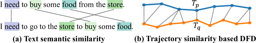
However, we argue that these common practices pay excessive attention to capturing long-term global dependency between two trajectories while ignoring point-wise similarity, which may potentially yield adverse effects. Instead, we should pay more attention to point-wise similarity in the local context. In support of this argument, we conducted an experiment on Porto111https://www.kaggle.com/competitions/pkdd-15-predict-taxi-service-trajectory-i/data dataset to evaluate the effect of applying Transformer for trajectory encoding with different sizes of attention windows. The first variant is the original Transformer with global attention, where each token engages in self-attention by querying all other tokens. We also implemented two alternative variants with local attention, in which each token only queries its neighbors within a window of count , i.e., the attention weights outside the window have been masked. We can observe from Table 1 that local attention has great potential to significantly outperform global attention. We explain that existing trajectory distance measurements are alignment-based and the edges for matching pairs are not intercrossed (as shown in Figure 1). This property differs significantly from handling text data in NLP.
These observations reveal the pivotal role of local similarity. Instead of adopting Transformer with masked local attention, we are interested in revisiting CNNs in the task of trajectory similarity learning. The reason is that CNNs can also well capture local similarity while offering the advantages of simplicity and smaller network structures. As shown in Table 1, with only of the parameters, a simple 1D CNN can remarkably outperform Transformers. To further exploit the potential of CNNs, we present ConvTraj with two types of convolutions. We first use 1D convolution to capture the sequential features of trajectories. Then we represent the trajectory as a single-channel binary image and use 2D convolution to capture its geo-distribution. Finally, these features are fused as complementary clues to capture trajectory similarity. To justify the effectiveness of ConvTraj, we conduct a series of theoretical analyses. We prove that 1D convolution and 1D max-pooling can preserve effective distance bounds after embedding, and trajectories located in distant areas yield large distances via 2D convolution, all of which play an important role in trajectory similarity recognition.
We conducted extensive experiments to evaluate the performance of ConvTraj on three real-world datasets. Experimental results show that ConvTraj achieves state-of-the-art accuracy for similarity retrieval on four commonly used similarity measurements, including DFD, DTW, Hausdorff, and EDR. Furthermore, ConvTraj is at least x faster in training speed and x faster in inference speed, when compared with methods based on RNN and Transformer on the Porto dataset containing 1.6 million trajectories.
Our contributions are summarized in the following:
-
•
We argue that trajectory similarity learning should pay more attention to local similarity.
-
•
We present a simple and effective ConvTraj with two types of CNNs for trajectory similarity computation.
-
•
We conduct some theoretical analysis to help justify why such a simple ConvTraj can perform well.
-
•
Extensive experiments on three real-world large-scale datasets established the superiority of ConvTraj over state-of-the-art works in terms of accuracy and efficiency.
2. Related Work
2.1. Heuristic Trajectory Similarity Measures
Heuristic measures between trajectories are derived from the distance between matching point pairs, these measures fall into three categories: (1) Linear-based methods (Agrawal et al., 1993; Chang et al., 2021) only need scan trajectories once to calculate their similarity but may lead to sub-optimal point matches. (2) Dynamic programming-based methods are proposed to tackle this issue, such as DTW (Yi et al., 1998), DFD (Alt and Godau, 1995), and others (Chen et al., 2005; Chen and Ng, 2004; Vlachos et al., 2002; Ranu et al., 2015). However, these measurements involve the optimal point-wise alignment between two trajectories without intercrossing between matching pairs and often incur quadratic complexity. Thus it poses significant challenges for similarity search from a large-scale dataset with long trajectories. (3) Enumeration-based methods calculate all point-to-trajectory distance, i.e., the minimum distance between a point to any point on a trajectory, then aggregate it. For example, OWD (Lin and Su, 2008) uses the average point-to-trajectory distance, while Hausdorff (Atev et al., 2010) uses the maximum.
2.2. Learning-based Trajectory Similarity
In recent years, the field of trajectory similarity has witnessed a paradigm shift, primarily fueled by the progress in deep representation learning. This advancement has led to the development of numerous methodologies aimed at encoding trajectories into embedding spaces. Broadly, these approaches can be classified into three categories: (1) Learn a model to approximate a measurement. The purpose of these methods is to learn a neural network so that the distance in the embedding space can approximate the true distance between trajectories. Early attempts were generally based on recurrent neural networks, including NeuTraj (Yao et al., 2019), Traj2SimVec (Zhang et al., 2020), T3S (Yang et al., 2021), and TMN (Yang et al., 2022). Subsequently, some studies tried to capture the long-term dependency of trajectories based on Transformer (Yao et al., 2022; Chang et al., 2023a). (2) No given measurements are required to generate training signals. These methods encode trajectories without the need to generate supervised signals based on measurements. Its purpose is to overcome the limitations of traditional measures such as non-uniform sampling rates and noise. Based on the network they use, these methods can be divided into RNN-based methods, including traj2vec (Yao et al., 2018), t2vec (Li et al., 2018), E2DTC (Fang et al., 2021), etc., CNN-based method TrjSR (Cao et al., 2021), and Transformer-based method TrajCL (Chang et al., 2023a). (3) Road networks-based methods. There have been some studies on trajectory similarity based on road networks (Han et al., 2021; Fang et al., 2022; Zhou et al., 2023a; Chang et al., 2023b; Zhou et al., 2023b). These works use graph neural networks to encode road segments. Since such works introduce relevant knowledge from road networks, we consider them as different research directions and will not delve into these methods.
TrjSR (Cao et al., 2021) is a well-known CNN-based method for trajectory similarity. It maps trajectories into 2D images and uses super-resolution techniques. However, TrjSR loses the sequential features of trajectories, making it unable to differentiate between two trajectories with the same path but opposite directions. Our ConvTraj uses both 1D and 2D convolutions as the backbone and achieves better results.
3. Problem Definition
In this section, we present the definition of our research problem.
Definition 0 (Trajectory).
A trajectory is a series of GPS points ordered based on timestamp , and each point is a location in a two-dimensional geographic space containing latitude and longitude. Formally, a trajectory containing points can be expressed as , where is the -th location.
Definition 0 (Trajectory Measure Embedding).
Given a specific trajectory similarity measure , trajectory measure embedding aims to learn an approximate projection function , such that for any pair of trajectories with , the distance in the embedding space approximates the true distance between and , i.e., . Besides, the vectors in the embedding space should maintain the distance order of true distance, i.e., for any three trajectories , , and , with , we should ensure that . Here, can be DFD, DTW, or any other measurements. At the same time, is a measure between high-dimensional embedding vectors in the embedding space, such as Euclidean distance, Cosine distance, etc.
4. Methodology
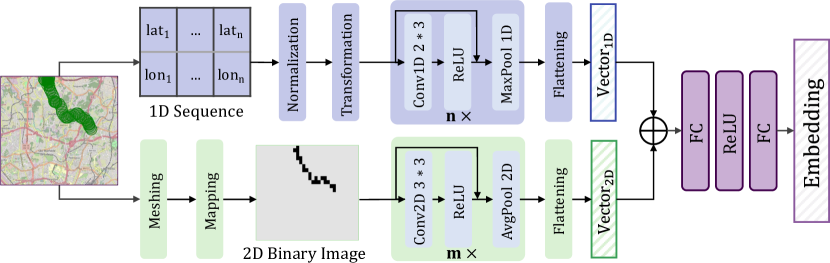
4.1. Input Preprocessing
Suppose there is a trajectory containing GPS points. To process as the input of our ConvTraj, we perform the following two steps covering both one-dimensional and two-dimensional.
One-dimensional Input. The input of our 1D convolution is a sequence, we thus treat the trajectory as a sequence with length and width 2 (i.e., latitude and longitude). For each point of , we first normalize it using a min-max normalization function, and then apply a multi-layer perceptron (MLP) to perform a nonlinear transformation for each normalization point, thus the trajectory can be processed as a sequence .
Two-dimensional Input. The input of our 2D convolution is a binary image, we thus perform the following substeps to generate such an image for each trajectory. Initially, we determine a minimum bounding rectangle (MBR) within a two-dimensional space, encapsulating all points of the whole trajectory dataset. Subsequently, the MBR is partitioned into equal-sized grids based on a predetermined hyperparameter width . Then for each trajectory , its coordinates are mapped onto the grid, and each pixel within the grid cell is assigned a binary value, which is 1 if the trajectory point falls within the grid cell and 0 otherwise. Thus each raw trajectory is converted into a single-channel binary image .
4.2. ConvTraj Network Structure
As shown in Figure 2, the ConvTraj consists of three submodules: 1D convolution, 2D convolution, and feature fusion. The 1D convolution extracts sequential features from the trajectory, while the 2D convolution captures its geo-distribution. The feature fusion module then combines these features for comprehensive analysis. Detailed descriptions of these submodules are provided below.
One-dimensional Convolution. As shown in Figure 2, 1D convolution is stacked by residual blocks consisting of a 1D convolution layer, a non-linear ReLU layer, and a max-pooling layer. Each operation is performed on rows of . By default, the convolution kernel size is , the number of channels is , the pooling stride is , and the number of stacking layers is determined by the maximum length of the trajectory in the dataset. In the end, the features of all channels are flattened into a vector .
Two-dimensional Convolution. 2D convolution is also stacked by residual blocks consisting of a 2D convolution layer, a non-linear ReLU layer, and an average-pooling layer. Each operation is performed on the single-channel binary image . By default, the convolution kernel size is , the number of channels is , the pooling stride is , and the number of stacking layers is . In the end, the features of all channels are flattened into a vector .
Feature Fusion. After performing 1D and 2D convolution on the trajectory in parallel, we concatenate the resulting feature vectors and pass them through an MLP. This submodule combines the sequence order features () extracted by 1D convolution with the geo-distribution features () extracted by 2D convolution, providing comprehensive information for similarity recognition. The final embedding of the trajectory can be formalized as:
| (1) |
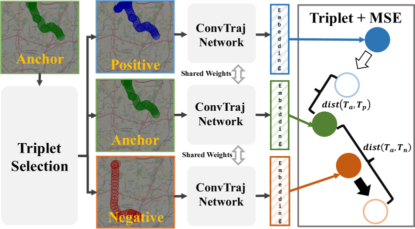
4.3. Training Pipeline
We employ the mainstream training pipeline as shown in Figure 3, and its details are introduced below.
Loss Function. As shown in Figure 3, we use the combination of triplet loss (Weinberger and Saul, 2009; Hermans et al., 2017) and MSE loss as our loss function. i.e.:
| (2) |
where
| (3) | |||
| (4) |
in which is a triplet, and is the anchor trajectory, is the positive trajectory that has a smaller distance to than the negative trajectory . , and are the high-dimensional vectors corresponding to , and in the embedding space. represents the true distance between trajectories, and is the Euclidean distance (Yao et al., 2019, 2022) between two vectors. Besides, is the margin in the triplet loss whose value is .
Triplet Selection Method. Many studies (Yao et al., 2019; Zhang et al., 2020; Yang et al., 2022) have proposed various strategies to select triplets for training, but these often bring additional training costs. In this paper, we use the simplest strategy to select triplets. We regard each trajectory in the training set as in turn. For each , we randomly select two trajectories from its top-k neighbors (k=200 by default) and use the trajectory closer to the as , and trajectory farther to as .
Training Process. Figure 3 is the overall training process of ConvTraj, where the blue hollow circle represents the location where the positive trajectory should be in the embedding space after training and the orange hollow circle represents the negative. During the training, for a trajectory (the anchor trajectory in the upper left corner of Figure 3), we first use the triplet selection method introduced above to select the positive trajectory (the blue trajectory in Figure 3) and negative trajectory (the orange trajectory in Figure 3), then these three trajectories are encoded using ConvTraj with shared parameters, and corresponding embedding vectors are obtained, which we call (green full circle), (blue full circle), (orange full circle). Since the loss function we use is a combination of triplet loss and MSE loss, we hope that the distance between anchor and positive in the embedding space is the same as the actual distance (i.e., pulling the blue full circle toward the blue hollow circle), and the distance between anchor and negative in embedding space is the same as the actual distance (i.e. pushing the orange full circle toward the orange hollow circle).
5. Theoretical Analysis
In this section, we will conduct some theoretical analysis from both 1D and 2D convolution to help justify why such a simple ConvTraj can perform well. We take the DFD, which is widely used for trajectory similarity (Zhang et al., 2022; Xie et al., 2017; Zhang et al., 2019; Tang et al., 2017), as an example for analysis. In summary, we found that: (1) For a randomly initialized kernel of 1D convolution, the DFD between two trajectories can still be maintained to a large extent. (2) After 1D max-pooling, the DFD value has almost no change. (3) Trajectories located in distant areas not only have a large DFD value but also have a large Euclidean distance through 2D convolution. Since 1D convolution essentially rotates and scales the sequence and 2D convolution captures the geo-distribution of trajectories, thus similar conclusions can be easily generalized to other measurements.
5.1. Discrete Frechet Distance
To facilitate understanding, we first present the formal definition of Discrete Frechet Distance:
Definition 0 (Trajectory Coupling).
A coupling between two trajectories and is such a sequence of alignment:
where . For all , we have or , and or .
Definition 0 (Discrete Frechet Distance).
Given two trajectories and , the Discrete Frechet Distance between these two trajectories is:
where is an instance of coupling between and , and is Euclidean distance between two points.
5.2. One-dimensional Convolution
Definition 0.
Given a trajectory and a kernel , we define the convolution operation of the point of with the kernel as:
where .
Theorem 5.4 (One-dimensional Convolution Bound).
Given two trajectories , , and . A one-dimensional convolution operation on and with stride 1, padding 1, and kernel . We have:
where ,
, and .
Proof.
Suppose that , where . Similarly, . Since , we assume that the coupling corresponding to is , and the indexs of and in are and . Then we apply to , thus:
where . Based on Cauchy–Schwarz inequality, we can get:
In addition, there is always such a coupling between and , thus:
The proof can be completed by rearranging the above formula. ∎
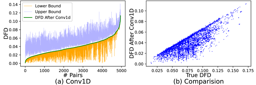
To verify the effectiveness of Theorem 5.4, we randomly selected 5000 pairs of trajectories from the Porto dataset for testing and randomly initialized a convolution kernel using PyTorch. The results in Figure 4a show that the DFD between the trajectories after 1D convolution can accurately fall between the bounds of our predictions by Theorem 5.4. In addition, there is a positive correlation between the true DFD and the DFD after 1D convolution in Figure 4b, which implies that even for a randomly initialized kernel, the DFD can still be maintained to a large extent.
Theorem 5.5 (One-dimensional Max-Pooling Bound).
Given two sequences , , and each is a -dimensional vector, i.e., . A one-dimensional max pooling operation on with size and stride , assuming that and are divisible by . Then the following holds:
in which
and , ; , .(The same goes for and )
Proof.
Based on the triangle inequality of DFD, we can get:
Using this property again, we have:
Rearrange these two inequalities, we can get:
Suppose , and each is a -dimensional vector, i.e., , where . Then for , we can always construct such a coupling . Thus . In this way, we divide the coupling into groups. Without loss of generality, we take out the -th group, that is:
thus for , we have:
Using this bound to completes the proof. ∎
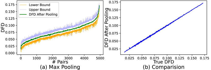
To verify the effectiveness of Theorem 5.5, we use the same setting as Theorem 5.4 for testing. The size and stride of max-pooling are set to 2, i.e., . As shown in Figure 5a, the DFD between the trajectories after max-pooling can also accurately fall between the bounds of our predictions by Theorem 5.5. In addition, Figure 5b shows that the real DFD value has almost no change compared with the DFD after max-pooling, this implies that max-pooling is a suitable technique that can reduce the dimensionality of trajectory sequences with almost no loss of effective features that are important for DFD-based similarity recognition.
5.3. Two-dimensional Convolution
Definition 0 (Trajectory MBR Distance).
Given two trajectories and , we denote the Minimum Bounding Rectangles (MBRs) of and as and based on the minimum and maximum longitude and latitude of the trajectory. We thus define the distance between and is:
where is Euclidean distance between two points.
Theorem 5.7 (Two-dimensional Convolution Bound).
Given two trajectories and , their MBRs are and . We denote the binary images of and based on the grid width as , , and the non-0 pixels contained in and are and respectively. A two-dimensional convolution operation on and with stride 1, padding 1, kernel . If , then we have , and
where is Euclidean distance between two vectors.
Proof.
We can easily get based on , thus:
Due to , there must be:
Since stride and padding are 1, we can easily deduce that there is no overlap between and , thus:
Considering that is essentially a superposition of kernels at different locations, and , thus in any case there is:
Applying this bound to completes the proof. ∎
6. Experiments
6.1. Experimental Setting
Datasets. We evaluate the performance of ConvTraj using three widely used real-world datasets: Geolife222https://www.microsoft.com/en-us/research/publication/geolife-gps-trajectory-dataset-user-guide/, Porto333https://www.kaggle.com/competitions/pkdd-15-predict-taxi-service-trajectory-i/data and TrajCL-Porto444https://github.com/changyanchuan/TrajCL. For Geolife and Porto, we preprocess them using the method in (Yao et al., 2019), i.e. selecting trajectories in the central area of the city and removing items with less than 10 records. For TrajCL-Porto, it’s an open-source dataset of TrajCL(Chang et al., 2023a), we thus do not perform any processing. The properties of these datasets are shown in Table 2.
| Dataset | Geolife | Porto | TrajCL-Porto |
| # Total Items | |||
| # Training Items | |||
| # Query Items | |||
| # Candidate Items | |||
| Avg-(# GPS Points) | |||
| Min-(# GPS Points) | |||
| Max-(# GPS Points) | |||
| Lat and Lon Area | (116.20, 116.50) (39.85, 40.07) | (-8.73, -8.50) (41.10, 41.24) | (-8.70, -8.52) (41.10, 41.208) |
| Geolife | ||||||||||
| Hausdorff | DFD | |||||||||
| Model | HR@1 | HR@5 | HR@10 | HR@50 | R10@50 | HR@1 | HR@5 | HR@10 | HR@50 | R10@50 |
| t2vec | ||||||||||
| TrjSR | ||||||||||
| TrajCL | ||||||||||
| NeuTraj | ||||||||||
| Traj2SimVec | ||||||||||
| TrajGAT | ||||||||||
| ConvTraj | ||||||||||
| Gap with SOTA | ||||||||||
| DTW | EDR | |||||||||
| t2vec | ||||||||||
| TrjSR | ||||||||||
| TrajCL | ||||||||||
| NeuTraj | ||||||||||
| Traj2SimVec | ||||||||||
| TrajGAT | ||||||||||
| ConvTraj | ||||||||||
| Gap with SOTA | ||||||||||
| Porto | ||||||||||
| Hausdorff | DFD | |||||||||
| Model | HR@1 | HR@5 | HR@10 | HR@50 | R10@50 | HR@1 | HR@5 | HR@10 | HR@50 | R10@50 |
| t2vec | ||||||||||
| TrjSR | ||||||||||
| TrajCL | ||||||||||
| NeuTraj | ||||||||||
| Traj2SimVec | ||||||||||
| TrajGAT | ||||||||||
| ConvTraj | ||||||||||
| Gap with SOTA | ||||||||||
| DTW | EDR | |||||||||
| t2vec | ||||||||||
| TrjSR | ||||||||||
| TrajCL | ||||||||||
| NeuTraj | ||||||||||
| Traj2SimVec | ||||||||||
| TrajGAT | ||||||||||
| ConvTraj | ||||||||||
| Gap with SOTA | ||||||||||
| TrajCL-Porto | ||||||||||||
| EDR | EDwP | Hausdorff | DFD | |||||||||
| Model | HR@5 | HR@20 | R5@20 | HR@5 | HR@20 | R5@20 | HR@5 | HR@20 | R5@20 | HR@5 | HR@20 | R5@20 |
| t2vec | ||||||||||||
| TrjSR | ||||||||||||
| E2DTC (Fang et al., 2021) | ||||||||||||
| CSTRM (Liu et al., 2022) | ||||||||||||
| TrajCL | 0.222 | |||||||||||
| T3S (Yang et al., 2021) | ||||||||||||
| Traj2SimVec | ||||||||||||
| TrajGAT | ||||||||||||
| ConvTraj | 0.292 | 0.414 | 0.776 | 0.826 | 0.987 | 0.754 | 0.770 | 0.983 | 0.760 | 0.786 | 0.984 | |
| Gap with SOTA | ||||||||||||
| ConvTraj-1D CNN | ||||||||||||
| ConvTraj-2D CNN | ||||||||||||
Baselines. When we test on Geolife and Porto, we follow existing works (Yao et al., 2022; Chang et al., 2023c) and compare ConvTraj with six representative methods, including t2vec (Li et al., 2018) and TrjSR (Cao et al., 2021) based on self-supervised learning; NeuTraj (Yao et al., 2019), Traj2SimVec (Zhang et al., 2020), TrajGAT (Yao et al., 2022), and TrajCL (Chang et al., 2023a) based on supervised learning. For the self-supervised method, since its goal is not to approximate the existing measurements, we thus perform the following steps to handle it. We first randomly select a part of the trajectory for pre-training (We select 10000 trajectories for Geolife and 200000 for Porto. Since TrajCL also needs pre-training, we will use these data to pre-train TrajCL). Then we add an MLP encoder in the end and fine-tune it with the triplet selection method and loss function in subsection 4.3. For those methods which have open-source code (Li et al., 2018; Chang et al., 2023a; Yao et al., 2019, 2022; Cao et al., 2021), we directly use their implementation. For others (Zhang et al., 2020), we implement it based on the settings of its paper.
In addition, since many baselines have been evaluated on the TrajCL-Porto and the results have been reported in (Chang et al., 2023a), we will directly compare the results of ConvTraj on TrajCL-Porto with those of other baselines reported in (Chang et al., 2023a).
Metrics. We follow existing works (Yao et al., 2019; Zhang et al., 2020; Yao et al., 2022) and evaluate the effectiveness of these methods using the task of nearest neighbor search. Specifically, we first use the top- hitting rate (HR@), which is the overlap percentage of detection top- results with the ground truth. The second is the top-50 recall of the top-10 ground truth (R10@50), i.e. how many top 10 ground truths are recovered by the generated top 50 lists. The calculation of these two types of metrics is very close. For HR@, we first find the top- most similar trajectories for each query in the candidate set. Then, for each query, trajectories in the candidate set are ranked according to their distance to the query in the embedding space. If the trajectories ranking top contain of the true top- neighbors, the HR@ is . For R10@50, we first find the top 10 most similar trajectories for each query in the candidate set. Then, for each query, trajectories in the candidate set are ranked according to their distance to the query in the embedding space. Similarly, if the trajectories ranking top 50 contain of the true top-10 neighbors, the R10@50 is . These metrics can effectively evaluate whether the distance order in the embedding space is still preserved.
Implementation Details. We set the MLP output dimension in 1D preprocessing to 16, and grid width when generating binary images. For the Geolife dataset, the number of residual blocks for 1D convolution is , Porto is , and TrajCl-Porto is . During training, we set the batch size to 128, the learning rate to , and the embedding dimension to 128. We evaluated four common trajectory similarity measurements, Hausdorff, DFD, DTW, and EDR on Geolife and Porto, and evaluated Hausdorff, DFD, EDwP (Ranu et al., 2015), and EDR on TrajCL-Porto. For each measurement on Geolife and Porto, we select three random seeds to repeat the experiment and report the average result and variance. All experiments are conducted on a machine equipped with 36 CPU cores (Intel Core i9-10980XE CPU with 3.00GHz), 256 GB RAM, and a GeForce RTX 3090Ti GPU.
| Geolife | Porto | ||||||||
| Method | Paras | Pre-trained time * ( epoch) | Train time * ( epoch) | Train time Per Epoch | Inference time | Pre-trained time * ( epoch) | Train time * ( epoch) | Train time Per Epoch | Inference time |
| t2vec | M | s * | s * | s | s | s * | s * | s | s |
| TrjSR | s * | s * | s | 0.09s | s * | s * | s | 11.69s | |
| TrajCL | M | s * | s * | s | s | s * | s * | s | s |
| NeuTraj | M | - | s * | s | s | - | s * | s | s |
| TrajGAT | M | - | s * | s | s | - | s * | s | s |
| ConvTraj | M | - | s * | 1.57s | s | - | s * | 1.07s | s |
6.2. Effectiveness
Table 3 and Table 4 present an overview of the performance exhibited by different methods concerning the top- similarity search task on Geolife and Porto, we can observe that: (1) On both Geolife and Porto datasets, ConvTraj significantly outperforms all methods on all metrics. Taking the Hausdorff distance on the Geolife as an example, compared with the state-of-the-art baseline NeuTraj, ConvTraj exceeds by more than 11% in all metrics, with the largest improvement of 15.42% for HR@5 and the smallest improvement of 11.64% for HR@1. In addition, even for the Porto which contains 1.6 million trajectories, R10@50 has at least a 10.75% improvement on four measurements. This non-negligible improvement in performance is impressive given the fact that the sequence order features extracted by 1D convolution and the geographical distribution of the trajectory extracted by 2D convolution are both very beneficial to generating high-quality trajectory embedding representations. (2) The advantage of ConvTraj is evident in all measurements, which shows that ConvTraj is a general framework for different measurements. We can observe that no method can handle all measurements well. For example, NeuTraj performs best on the Hausdorff and DFD, while TrjSR and TrajCL have advantages on DTW and EDR respectively, which is also mutually verified with the results in (Chang et al., 2023c). However, ConvTraj achieves state-of-the-art accuracy in all measurements. Compared to the state-of-the-art, ConvTraj achieves an average improvement of 10.22%, 8.02%, 7.59%, and 7.03% on all metrics of the Hausdorff, DFD, DTW, and EDR in Porto respectively.
Table 5 presents the experimental results on TrajCL-Porto, we can observe that: (1) Similar to its performance on the Geolife and Porto, the ConvTraj method surpasses state-of-the-art in almost all metrics for four measurements. Compared with the state-of-the-art, Convtraj achieves improvements of 12%, 23%, 6.8%, and 14.2% on the HR@5 metrics of EDR, EDwP, Hausdorff, and DFD. (2) Even though both were tested on the Porto dataset, the performance gap between Table 3, Table 4 and Table 5 is very large. For example, the HR@5 of the TrajCL and ConvTraj in Table 5 on the DFD are 0.618 and 0.749 respectively, but in Table 4 they are 0.141 and 0.349 respectively. The reason is that the TrajCL-Porto dataset contains fewer trajectories. When performing the top- similarity search task, the TrajCL-Porto dataset only has 2000 candidate trajectories. However, the Porto used in Table 3 and Table 4 contains 1598079 candidate trajectories, which results in a more comprehensive result. (3) We also evaluate the performance of ConvTraj using only 1D convolution (ConvTraj-1D CNN) or 2D convolution (ConvTraj-2D CNN) on TrajCL-Porto, and we can observe that ConvTraj’s performance degrades after missing some features, but still has excellent performance.
| Haus | DFD | DTW | EDR | ||||||||||
| Method | HR@10 | HR@50 | R10@50 | HR@10 | HR@50 | R10@50 | HR@10 | HR@50 | R10@50 | HR@10 | HR@50 | R10@50 | |
| Geolife | 1D CNN | ||||||||||||
| 2D CNN | |||||||||||||
| 1D + 2D | 63.69 | 76.12 | 95.20 | 68.86 | 79.52 | 97.34 | 46.46 | 59.26 | 83.70 | 28.64 | 30.75 | 54.93 | |
| Porto | 1D CNN | ||||||||||||
| 2D CNN | |||||||||||||
| 1D + 2D | 33.27 | 45.98 | 67.20 | 40.59 | 53.35 | 77.33 | 24.46 | 35.36 | 52.83 | 15.61 | 21.45 | 37.00 | |
| Hausdorff | DFD | DTW | EDR | ||||||||||
| Method | HR@10 | HR@50 | R10@50 | HR@10 | HR@50 | R10@50 | HR@10 | HR@50 | R10@50 | HR@10 | HR@50 | R10@50 | |
| Porto-S-10 | 2D CNN | ||||||||||||
| LSTM+2D | 99.90 | 86.60 | 95.36 | 99.66 | 47.26 | 45.56 | |||||||
| 1D+2D | 80.40 | 88.64 | 99.78 | 83.02 | 88.84 | 99.66 | 85.20 | ||||||
| Porto-S-70 | 2D CNN | ||||||||||||
| LSTM+2D | |||||||||||||
| 1D+2D | 72.22 | 79.67 | 99.24 | 72.64 | 78.60 | 98.88 | 72.24 | 82.53 | 98.84 | 38.16 | 38.08 | 66.78 | |
| Porto-S | 2D CNN | ||||||||||||
| LSTM+2D | 97.44 | ||||||||||||
| 1D+2D | 65.04 | 73.76 | 58.22 | 68.20 | 94.70 | 57.42 | 67.64 | 94.44 | 25.62 | 28.82 | 53.14 | ||
6.3. Efficiency
We evaluate the efficiency of all baselines with open-source implementations and report the results in Table 6. This includes network parameters, training time, and inference time. For methods that require pre-training, we also report their pre-training time. As illustrated, compared to existing RNN-based and Transformer-based methods, ConvTraj not only has fewer parameters (only 0.03M more than NeuTraj) but also has great advantages in training and inference speed. Taking the Porto with 1.6 million items as an example, compared with the most efficient Transformer-based model TrajCL, the training speed per epoch and the inference speed of ConvTraj are at least 243.80x and 12.87x faster respectively. Compared with the most efficient RNN-based model t2vec, the training speed per epoch and the inference speed of ConvTraj are at least 306.91x and 2.16x faster respectively. The reason for such a huge improvement is that compared to Transformer-based methods, ConvTraj has fewer parameters. Meanwhile, compared with RNN-based methods, although the parameters of ConvTraj are relatively large, the training and inference of ConvTraj are more efficient due to the inherent low parallelism of RNN. In addition, we also note that: (1) Compared with the CNN-based TrjSR, ConvTraj has no advantage in inference, but the training is faster because TrjSR requires pre-training on a large number of trajectories, and only uses fewer convolutional layers during inference, which also shows the superiority of CNN in terms of efficiency. (2) Although both t2vec and NeuTraj are based on RNN, and NeuTraj has fewer parameters, t2vec is more efficient. The reason is that NeuTraj needs to select more triplets during the training phase and compute spatial attention based on adjacent grids at each time step.
6.4. Ablation Studies
6.4.1. The Role of 1D and 2D Convolution
Our ConvTraj combines 1D and 2D convolutions, we thus conducted the following experiments to evaluate the contributions of each module: (1) 1D CNN. Using only 1D convolution features. (2) 2D CNN. Using only 2D convolution features. (3) 1D+2D. Using 1D and 2D convolution together. The results in Table 7 show that for all measurements, neglecting any of these modules leads to a reduction in performance. In addition, we observe that 2D CNN outperforms most baselines, including TrjSR, which also uses 2D convolution. A similar conclusion can also be derived from Table 5. We explain that the goal of TrjSR is to reconstruct a high-resolution image from a low-resolution so that it can be as close as possible to the original image, thus the backbone and loss used are quite different from our 2D CNN. Furthermore, although we fine-tuned TrjSR, our 2D CNN is trained end-to-end and thus has more advantages.
6.4.2. Use LSTM to Replace 1D Convolution
In our ConvTraj, the role of 1D convolution is to capture the sequential features of trajectories. Although RNNs are commonly used for this purpose (Yao et al., 2019), we aim to demonstrate the important role of 1D convolution in ConvTraj by replacing it with an LSTM network. We will compare three methods to show the effectiveness of 1D convolution in capturing sequential features: (1) 2D CNN. Only using 2D convolution. (2) LSTM+2D. Using LSTM and 2D convolution together. (3) 1D+2D. Using 1D and 2D convolution together. The dataset used in this study is the same as Table 1, called Porto-S, and the number of GPS points contained in each trajectory in Porto-S ranges from 104 to 888. In addition, we generated two more datasets, Porto-S-10 and Porto-S-70, which contain the first 10 and 70 GPS points of each trajectory in Porto-S respectively, i.e., each trajectory in Porto-S-10 contains 10 GPS points, and each trajectory in Porto-S-70 contains 70 GPS points.
As shown in Table 8, the performance of LSTM+2D and 1D+2D is similar in the Porto-S-10, and LSTM+2D even performs slightly better than 1D+2D at some measurements (e.g., DTW and EDR), and both methods are significantly outperform than 2D CNN. These results show that LSTM performs very well in capturing sequential features when the trajectory contains fewer GPS points. However, as the number of points in a trajectory increases, the ability of LSTM to capture sequential features gradually decreases. For example, the HR@1 of 1D+2D and LSTM+2D on Porto-S-10 are 62.40% and 63.20% respectively for DTW. However, the HR@1 on Porto-S-70 are 52.40% and 46.40% respectively, and on Porto-S they are 38.60% and 22.20%. The gaps between them are -0.80%, +6.0%, +16.4%, and the gap gradually becomes larger. Even LSTM+2D has almost the same performance as using only 2D CNN on Porto-S. These results suggest that RNNs struggle to effectively capture the sequential features of trajectories with a large number of GPS points, whereas one-dimensional CNNs do not exhibit this limitation.
6.4.3. Loss Function Ablation Studies
In our ConvTraj, the loss function is the combination of triplet loss and MSE loss, where the role of MSE loss is to scale and approximate the trajectory distance, and triplet loss is to capture the relative similarity between trajectories. In order to demonstrate the role of these two loss functions in training, we conducted an ablation study on these two functions on the Geolife dataset. As shown in Table 9, we can clearly observe that after removing the triplet loss, all metrics have declined. However, after removing the MSE loss, the metrics of Hausdorff and DFD have declined, while the metrics of DTW and EDR have increased. We guess that the reason for this problem is that compared to Hausdorff and DFD, the range of distance values of DTW and EDR is relatively large. As shown in Table 10, the distance value ranges of Hausdorff and DFD are between 0~0.32 and 0~0.34 respectively, however, the value ranges of DTW and EDR are between 0~1289.4 and 0~6256.0. Such a huge gap may cause the MSE loss to encounter some problems during scaling. A more detailed discussion may be studied in future work.
| Method | HR@1 | HR@10 | HR@50 | R10@50 | |
| Haus | w/o Triplet | ||||
| w/o MSE | |||||
| Triplet + MSE | 46.17 | 63.69 | 76.12 | 95.20 | |
| DFD | w/o Triplet | ||||
| w/o MSE | |||||
| Triplet + MSE | 51.80 | 68.86 | 79.52 | 97.34 | |
| DTW | w/o Triplet | ||||
| w/o MSE | 34.00 | 47.16 | |||
| Triplet + MSE | 59.26 | 83.70 | |||
| EDR | w/o Triplet | ||||
| w/o MSE | 33.30 | 38.11 | 37.55 | 66.66 | |
| Triplet + MSE |
| Measurements | Hausdorff | DFD | DTW | EDR |
| Distance Value Range | 0~0.32 | 0~0.34 | 0~1289.4 | 0~6256.0 |
7. Conclusion
In this paper, we argue that trajectory similarity learning should pay more attention to local similarity. Then we propose a simple CNN-based framework ConvTraj. Some theoretical analysis is conducted to help justify the effectiveness of ConvTraj. Extensive experiments on three real-world datasets show the superiority of ConvTraj.
References
- (1)
- Agarwal et al. (2018) Pankaj K. Agarwal, Kyle Fox, Kamesh Munagala, Abhinandan Nath, Jiangwei Pan, and Erin Taylor. 2018. Subtrajectory Clustering: Models and Algorithms. In PODS. ACM, 75–87.
- Agrawal et al. (1993) Rakesh Agrawal, Christos Faloutsos, and Arun N. Swami. 1993. Efficient Similarity Search In Sequence Databases. In FODO (Lecture Notes in Computer Science), Vol. 730. Springer, 69–84.
- Alt and Godau (1995) Helmut Alt and Michael Godau. 1995. Computing the Fréchet distance between two polygonal curves. Int. J. Comput. Geom. Appl. 5 (1995), 75–91.
- Atev et al. (2010) Stefan Atev, Grant Miller, and Nikolaos P. Papanikolopoulos. 2010. Clustering of Vehicle Trajectories. IEEE Trans. Intell. Transp. Syst. 11, 3 (2010), 647–657.
- Cao et al. (2021) Hanlin Cao, Haina Tang, Yulei Wu, Fei Wang, and Yongjun Xu. 2021. On Accurate Computation of Trajectory Similarity via Single Image Super-Resolution. In IJCNN. IEEE, 1–9.
- Chan et al. (2018) T.-H. Hubert Chan, Arnaud Guerquin, and Mauro Sozio. 2018. Fully Dynamic k-Center Clustering. In WWW. ACM, 579–587.
- Chang et al. (2023a) Yanchuan Chang, Jianzhong Qi, Yuxuan Liang, and Egemen Tanin. 2023a. Contrastive Trajectory Similarity Learning with Dual-Feature Attention. In ICDE. IEEE, 2933–2945.
- Chang et al. (2021) Yanchuan Chang, Jianzhong Qi, Egemen Tanin, Xingjun Ma, and Hanan Samet. 2021. Sub-trajectory Similarity Join with Obfuscation. In SSDBM. ACM, 181–192.
- Chang et al. (2023b) Yanchuan Chang, Egemen Tanin, Xin Cao, and Jianzhong Qi. 2023b. Spatial Structure-Aware Road Network Embedding via Graph Contrastive Learning. In EDBT. OpenProceedings.org, 144–156.
- Chang et al. (2023c) Yanchuan Chang, Egemen Tanin, Gao Cong, Christian S. Jensen, and Jianzhong Qi. 2023c. Trajectory Similarity Measurement: An Efficiency Perspective. CoRR abs/2311.00960 (2023).
- Chen and Ng (2004) Lei Chen and Raymond T. Ng. 2004. On The Marriage of Lp-norms and Edit Distance. In VLDB. Morgan Kaufmann, 792–803.
- Chen et al. (2005) Lei Chen, M. Tamer Özsu, and Vincent Oria. 2005. Robust and Fast Similarity Search for Moving Object Trajectories. In SIGMOD. ACM, 491–502.
- Cho et al. (2014) Kyunghyun Cho, Bart van Merrienboer, Çaglar Gülçehre, Dzmitry Bahdanau, Fethi Bougares, Holger Schwenk, and Yoshua Bengio. 2014. Learning Phrase Representations using RNN Encoder-Decoder for Statistical Machine Translation. In EMNLP. ACL, 1724–1734.
- Fang et al. (2021) Ziquan Fang, Yuntao Du, Lu Chen, Yujia Hu, Yunjun Gao, and Gang Chen. 2021. EDTC: An End to End Deep Trajectory Clustering Framework via Self-Training. In ICDE. IEEE, 696–707.
- Fang et al. (2022) Ziquan Fang, Yuntao Du, Xinjun Zhu, Danlei Hu, Lu Chen, Yunjun Gao, and Christian S. Jensen. 2022. Spatio-Temporal Trajectory Similarity Learning in Road Networks. In KDD. ACM, 347–356.
- Han et al. (2021) Peng Han, Jin Wang, Di Yao, Shuo Shang, and Xiangliang Zhang. 2021. A Graph-based Approach for Trajectory Similarity Computation in Spatial Networks. In KDD. ACM, 556–564.
- Hermans et al. (2017) Alexander Hermans, Lucas Beyer, and Bastian Leibe. 2017. In defense of the triplet loss for person re-identification. arXiv preprint arXiv:1703.07737 (2017).
- Hochreiter and Schmidhuber (1997) Sepp Hochreiter and Jürgen Schmidhuber. 1997. Long Short-Term Memory. Neural Comput. 9, 8 (1997), 1735–1780.
- Laxhammar and Falkman (2014) Rikard Laxhammar and Göran Falkman. 2014. Online Learning and Sequential Anomaly Detection in Trajectories. IEEE Trans. Pattern Anal. Mach. Intell. 36, 6 (2014), 1158–1173.
- Li et al. (2018) Xiucheng Li, Kaiqi Zhao, Gao Cong, Christian S. Jensen, and Wei Wei. 2018. Deep Representation Learning for Trajectory Similarity Computation. In ICDE. IEEE Computer Society, 617–628.
- Lin and Su (2008) Bin Lin and Jianwen Su. 2008. One Way Distance: For Shape Based Similarity Search of Moving Object Trajectories. GeoInformatica 12, 2 (2008), 117–142.
- Liu et al. (2022) Xiang Liu, Xiaoying Tan, Yuchun Guo, Yishuai Chen, and Zhe Zhang. 2022. CSTRM: Contrastive Self-Supervised Trajectory Representation Model for trajectory similarity computation. Comput. Commun. 185 (2022), 159–167.
- Ranu et al. (2015) Sayan Ranu, Deepak P, Aditya D. Telang, Prasad Deshpande, and Sriram Raghavan. 2015. Indexing and matching trajectories under inconsistent sampling rates. In ICDE, Johannes Gehrke, Wolfgang Lehner, Kyuseok Shim, Sang Kyun Cha, and Guy M. Lohman (Eds.). IEEE Computer Society, 999–1010.
- Shang et al. (2018) Zeyuan Shang, Guoliang Li, and Zhifeng Bao. 2018. DITA: Distributed In-Memory Trajectory Analytics. In SIGMOD. ACM, 725–740.
- Tang et al. (2017) Bo Tang, Man Lung Yiu, Kyriakos Mouratidis, and Kai Wang. 2017. Efficient Motif Discovery in Spatial Trajectories Using Discrete Fréchet Distance. In EDBT. OpenProceedings.org, 378–389.
- Vlachos et al. (2002) Michail Vlachos, Dimitrios Gunopulos, and George Kollios. 2002. Discovering Similar Multidimensional Trajectories. In ICDE, Rakesh Agrawal and Klaus R. Dittrich (Eds.). IEEE Computer Society, 673–684.
- Weinberger and Saul (2009) Kilian Q Weinberger and Lawrence K Saul. 2009. Distance metric learning for large margin nearest neighbor classification. Journal of machine learning research 10, 2 (2009).
- Xie et al. (2017) Dong Xie, Feifei Li, and Jeff M. Phillips. 2017. Distributed Trajectory Similarity Search. Proc. VLDB Endow. 10, 11 (2017), 1478–1489.
- Yang et al. (2022) Peilun Yang, Hanchen Wang, Defu Lian, Ying Zhang, Lu Qin, and Wenjie Zhang. 2022. TMN: Trajectory Matching Networks for Predicting Similarity. In ICDE. IEEE, 1700–1713.
- Yang et al. (2021) Peilun Yang, Hanchen Wang, Ying Zhang, Lu Qin, Wenjie Zhang, and Xuemin Lin. 2021. T3S: Effective Representation Learning for Trajectory Similarity Computation. In ICDE. IEEE, 2183–2188.
- Yao et al. (2019) Di Yao, Gao Cong, Chao Zhang, and Jingping Bi. 2019. Computing Trajectory Similarity in Linear Time: A Generic Seed-Guided Neural Metric Learning Approach. In ICDE. IEEE, 1358–1369.
- Yao et al. (2022) Di Yao, Haonan Hu, Lun Du, Gao Cong, Shi Han, and Jingping Bi. 2022. TrajGAT: A Graph-based Long-term Dependency Modeling Approach for Trajectory Similarity Computation. In SIGKDD. ACM, 2275–2285.
- Yao et al. (2018) Di Yao, Chao Zhang, Zhihua Zhu, Qin Hu, Zheng Wang, Jian-Hui Huang, and Jingping Bi. 2018. Learning deep representation for trajectory clustering. Expert Syst. J. Knowl. Eng. 35, 2 (2018).
- Yi et al. (1998) Byoung-Kee Yi, H. V. Jagadish, and Christos Faloutsos. 1998. Efficient Retrieval of Similar Time Sequences Under Time Warping. In ICDE. IEEE Computer Society, 201–208.
- Zhang et al. (2022) Dongxiang Zhang, Zhihao Chang, Sai Wu, Ye Yuan, Kian-Lee Tan, and Gang Chen. 2022. Continuous Trajectory Similarity Search for Online Outlier Detection. IEEE Trans. Knowl. Data Eng. 34, 10 (2022), 4690–4704.
- Zhang et al. (2020) Hanyuan Zhang, Xinyu Zhang, Qize Jiang, Baihua Zheng, Zhenbang Sun, Weiwei Sun, and Changhu Wang. 2020. Trajectory Similarity Learning with Auxiliary Supervision and Optimal Matching. In IJCAI. ijcai.org, 3209–3215.
- Zhang et al. (2019) Jiahao Zhang, Bo Tang, and Man Lung Yiu. 2019. Fast Trajectory Range Query with Discrete Frechet Distance. In EDBT. OpenProceedings.org, 634–637.
- Zhou et al. (2023a) Silin Zhou, Peng Han, Di Yao, Lisi Chen, and Xiangliang Zhang. 2023a. Spatial-temporal fusion graph framework for trajectory similarity computation. WWW 26, 4 (2023), 1501–1523.
- Zhou et al. (2023b) Silin Zhou, Jing Li, Hao Wang, Shuo Shang, and Peng Han. 2023b. GRLSTM: Trajectory Similarity Computation with Graph-Based Residual LSTM. In AAAI. AAAI Press, 4972–4980.