Identifiability of a statistical model with two latent vectors: Importance of the dimensionality relation and application to graph embedding

Hiroaki Sasaki
Department of Mathematical Informatics
Meiji Gakuin University, Japan
Abstract

Identifiability of statistical models is a key notion in unsupervised representation learning. Recent work of nonlinear independent component analysis (ICA) employs auxiliary data and has established identifiable conditions. This paper proposes a statistical model of two latent vectors with single auxiliary data generalizing nonlinear ICA, and establishes various identifiability conditions. Unlike previous work, the two latent vectors in the proposed model can have arbitrary dimensions, and this property enables us to reveal an insightful dimensionality relation among two latent vectors and auxiliary data in identifiability conditions. Furthermore, surprisingly, we prove that the indeterminacies of the proposed model has the same as linear ICA under certain conditions: The elements in the latent vector can be recovered up to their permutation and scales. Next, we apply the identifiability theory to a statistical model for graph data. As a result, one of the identifiability conditions includes an appealing implication: Identifiability of the statistical model could depend on the maximum value of link weights in graph data. Then, we propose a practical method for identifiable graph embedding. Finally, we numerically demonstrate that the proposed method well-recovers the latent vectors and model identifiability clearly depends on the maximum value of link weights, which supports the implication of our theoretical results.

1 Introduction

Unsupervised representation learning is a big issue in machine learning (Raina et al.,, 2007; Bengio et al.,, 2013): Data representation learned from a large amount of unlabeled data has been applied for downstream tasks to improve the performance. Empirical successes of unsupervised representation learning have been reported in a number of works such as classification (Klindt et al.,, 2020), natural language processing (Peters et al.,, 2018; Devlin et al.,, 2019), graph embedding Cai et al., (2018). On the other hand, it is often theoretically challenging to understand how representation of data is learned.

One of the key notions in unsupervised representation learning is identifiability of statistical models. A seminar work is linear independent component analysis (ICA) (Comon,, 1994) where data vectors are generated from a linear mixing of latent variables. It has been proved than the latent variables can be identified from observed data vectors up to their permutation and scales. The fundamental conditions in linear ICA are statistical independence and nonGaussianity of the latent variables. The natural extension of linear ICA is nonlinear ICA where a general nonlinear function of latent variables is assumed in data generation. However, it has been shown that nonlinear ICA is considerably difficult under the same independence condition as linear ICA because there exist an infinite number of independent representations of data (Hyvärinen and Pajunen,, 1999; Locatello et al.,, 2019).

More recently, identifiable statistical models of single latent vectors have been proved in nonlinear ICA (Hyvärinen and Morioka,, 2016; Hyvärinen et al.,, 2019; Sasaki and Takenouchi,, 2022). In contrast with linear ICA, these works assume to have additional data called the auxiliary data, and make a conditional independence condition of latent variables given auxiliary data, which is alternative to the independent condition in linear ICA. Based on these conditions, it has been proved that latent variables are identifiable up to their permutation and elementwise nonlinear functions. Since then, a variety of nonlinear ICA methods haven been proposed such as time series data (Hyvärinen and Morioka,, 2017) and variational autoencoder (Khemakhem et al., 2020a, ), and applied to causal analysis (Monti et al.,, 2020; Wu and Fukumizu,, 2020) and transfer learning (Teshima et al.,, 2020). However, in nonlinear ICA, the indeterminacy of the elementwise nonlinear functions might make interpretation of the learned representation of data difficult even for simulated artificial data.

This paper proposes a new statistical model of two latent vectors with single auxiliary data and establishes identifiability conditions for one or both of the two latent vectors. Previously, an energy-based model (EBM) (Sasaki and Hyvärinen,, 2018; Khemakhem et al., 2020b, ) related to two latent vectors has been proposed. EBM makes use of statistical dependency of the two latent vectors in identifiability conditions, and assumes that these two vectors have the same dimension. In contrast, the proposed model allows these latent vectors to have different dimensions. Furthermore, thanks to additional auxiliary data, unlike EBM, these latent vectors are not necessarily dependent and can be even independent. Thus, our statistical model is very flexible. This flexibility reveals interesting dimensionality conditions between these latent vectors and auxiliary data: For instance, if one wants to recover one latent vector, then the dimensionality of the other latent vector should be equal to or larger than that of the target latent vector. In addition, we show that the indeterminacies of our model are the same as linear ICA under certain conditions. Therefore, surprisingly, the indeterminacies are simply permutation and scales of the elements in the latent vector, while data vectors are generated as a nonlinear mixing of latent variables. This is a significant step to interpret data representation in the identifiable models.

A promising application of the proposed statistical model is graph data, which consists of data vectors associated with nodes and their discrete link weights. By assuming that data vectors are generated from latent vectors, applying our identifiability theory to graph data includes an appealing implication: In order to recover the latent vectors underlying data, the maximum value of link weights should be large relative to the dimensionality of the latent vector. Based on the identifiability conditions, we propose a practical method for identifiable graph embedding called graph component analysis (GCA). Numerical experiments through GCA supports our theoretical implication and demonstrates that the performance of GCA clearly depends on the the maximum value of link weights.

2 Data generative model of two latent vectors

This section proposes a statistical model of two latent vectors with single auxiliary data. Given either discrete or continuous auxiliary data $\bm{w}\in\mathcal{W}\subset\mathbb{R}^{d_{\mathrm{w}}}$ with the marginal distribution $p_{\mathrm{w}}(\bm{w})$, we assume that two vectors of continuous latent variables, $\bm{s}=(s^{(1)},\dots,s^{(d_{\mathrm{s}})})^{\top}\in\mathbb{R}^{d_{\mathrm{s}}}$ and $\bm{v}=(v^{(1)},\dots,v^{(d_{\mathrm{v}})})^{\top}\in\mathbb{R}^{d_{\mathrm{v}}}$, follow the conditional distribution $p_{\mathrm{sv}|\mathrm{w}}(\bm{s},\bm{v}|\bm{w})$. Then, two data vectors $\bm{x}\in\mathbb{R}^{d_{\mathrm{x}}}$ and $\bm{u}\in\mathbb{R}^{d_{\mathrm{u}}}$ are generated from

$\displaystyle\bm{x}=\bm{f}(\bm{s})~{}~{}\text{and}~{}~{}\bm{u}=\bm{\varphi}(\bm{v}),$ (1)

where $\bm{f}:\mathbb{R}^{d_{\mathrm{s}}}\to{\mathbb{R}^{d_{\mathrm{x}}}}$ and $\bm{\varphi}:\mathbb{R}^{d_{\mathrm{v}}}\to{\mathbb{R}^{d_{\mathrm{u}}}}$ are nonlinear mixing functions with $d_{\mathrm{s}}\leq{d_{\mathrm{x}}}$ and $d_{\mathrm{v}}\leq{d_{\mathrm{u}}}$. We specifically assume that $\bm{f}$ and $\bm{\varphi}$ are smooth embeddings111A smooth embedding is a smooth immersion that is homeomorphism on its image (Lee,, 2012).. Thus, $\bm{f}$ and $\bm{\varphi}$ are continuous and bijective functions with smooth inverse to their images, which are denoted by

$\displaystyle\mathcal{M}_{\bm{f}}$ $\displaystyle:=\{\bm{x}=\bm{f}(\bm{s})~{}|~{}\bm{s}\in\mathbb{R}^{d_{\mathrm{s}}}\}\subset\mathbb{R}^{d_{\mathrm{x}}}$
$\displaystyle\mathcal{M}_{\bm{\varphi}}$ $\displaystyle:=\{\bm{u}=\bm{\varphi}(\bm{v})~{}|~{}\bm{v}\in\mathbb{R}^{d_{\mathrm{v}}}\}\subset\mathbb{R}^{d_{\mathrm{u}}}.$

Proposition 5.2 in Lee, (2012) allows us to regard $\mathcal{M}_{\bm{f}}$ and $\mathcal{M}_{\bm{\varphi}}$ as embedded submanifolds of $\mathbb{R}^{d_{\mathrm{x}}}$ and $\mathbb{R}^{d_{\mathrm{u}}}$, respectively.

A motivating example of this latent variable model is graph embedding (Cai et al.,, 2018). The goal of graph embedding is to learn an embedding function from data vectors associated with nodes and their link weights (i.e., graph data), which could be interpreted as an estimate of the inverse of $\bm{f}$ or $\bm{\varphi}$ in (1). Thus, graph embedding can be seen as unsupervised representation learning for graph data. By regarding two data vectors at a pair of nodes (e.g., $\bm{x}$ and $\bm{x}^{\prime}$) and link weight (e.g., $w$) as $\bm{x},\bm{u}$ and $\bm{w}$ in our model respectively, the proposed model includes a latent variable model for graph data as a special case. By applying our results, we establish identifiability conditions for graph data one of which includes an appealing implication.

Let us clarify that the observable variables are $\bm{w}$, $\bm{x}$ and $\bm{u}$, while $\bm{s}$ and $\bm{v}$ are latent variables and cannot be directly observed. Next, after defining the notion of identifiability for this statistical model, we establish the identifiability conditions.

3 Identifiability theory

We first define the notion of identifiability in this paper, and then establish various identifiability conditions.

3.1 Definition of identifiability

Here, the definition of identifiability is given. Since $\bm{f}$ and $\bm{\varphi}$ are smooth embeddings (i.e., continuous and bijective functions) to $\mathcal{M}_{\bm{f}}$ and $\mathcal{M}_{\bm{\phi}}$, we express $\bm{s}$ and $\bm{v}$ as

$\displaystyle\bm{s}=\bm{g}(\bm{x})~{}~{}\text{and}~{}~{}\bm{v}=\bm{\phi}(\bm{u}),$ (2)

where $\bm{g}:\mathcal{M}_{\bm{f}}\to\mathbb{R}^{d_{\mathrm{s}}}$ and $\bm{\phi}:\mathcal{M}_{\bm{\phi}}\to\mathbb{R}^{d_{\mathrm{s}}}$ are the inverses of $\bm{f}$ and $\bm{\varphi}$, respectively. By supposing the Euclidean metric both in the latent spaces of $\bm{s}$ and $\bm{v}$, (2) enables us to express the conditional distribution of $\bm{x}\in\mathcal{M}_{\bm{f}}$ and $\bm{u}\in\mathcal{M}_{\bm{\varphi}}$ given $\bm{w}$ (Gemici et al.,, 2016) as

$\displaystyle p_{\mathrm{xu}|\mathrm{w}}^{\bm{g},\bm{\phi}}(\bm{x},\bm{u}|\bm{w})=p_{\mathrm{sv}|\mathrm{w}}(\bm{g}(\bm{x}),\bm{\phi}(\bm{u})|\bm{w})\sqrt{\det(\bm{G}_{\bm{g}}(\bm{x}))}\sqrt{\det(\bm{G}_{\bm{\phi}}(\bm{u}))},$ (3)

where $\bm{G}_{\bm{g}}(\bm{x}):=\bm{J}_{\bm{g}}(\bm{x})^{\top}\bm{J}_{\bm{g}}(\bm{x})$ and $\bm{G}_{\bm{\phi}}(\bm{u}):=\bm{J}_{\bm{\phi}}(\bm{u})^{\top}\bm{J}_{\bm{\phi}}(\bm{u})$. Then, the notion of partially identifiability is defined as follows: $p_{\mathrm{xu}|\mathrm{w}}^{\bm{g},\bm{\phi}}$ is said to be partially identifiable with respective to $\bm{g}$ when

$\displaystyle p_{\mathrm{xu}|\mathrm{w}}^{\bm{g},\bm{\phi}}(\bm{x},\bm{u}|\bm{w})$ $\displaystyle=p_{\mathrm{xu}|\mathrm{w}}^{\tilde{\bm{g}},\tilde{\bm{\phi}}}(\bm{x},\bm{u}|\bm{w})~{}~{}\Rightarrow~{}~{}\bm{g}=\tilde{\bm{g}}.$ (4)

The partial identifiability might be sufficient in many practical situations, yet we also define an even stronger notion called the full identifiability: If

$\displaystyle p_{\mathrm{xu}|\mathrm{w}}^{\bm{g},\bm{\phi}}(\bm{x},\bm{u}|\bm{w})$ $\displaystyle=p_{\mathrm{xu}|\mathrm{w}}^{\tilde{\bm{g}},\tilde{\bm{\phi}}}(\bm{x},\bm{u}|\bm{w})~{}\Rightarrow~{}\bm{g}=\tilde{\bm{g}}~{}~{}\text{and}~{}~{}\bm{\phi}=\tilde{\bm{\phi}},$ (5)

$p_{\mathrm{xu}|\mathrm{w}}^{\bm{g},\bm{\phi}}$ is said to be fully identifiable. It follows from the definition that the full identifiability guarantees that one can estimate $\bm{g}$ and $\bm{\phi}$ through estimation of the conditional distribution of $\bm{x}$ and $\bm{u}$ given $\bm{w}$. Let us note that the recovery of two (single) latent vectors is almost a synonym of full (partial) identifiability by (2) in this paper. Next, we establish various conditions for partial and full identifiability.

3.2 Partial identifiability

We first show some conditions for partial identifiability with respect to $\bm{g}$. Note that the results can be easily converted to partial identifiability with respect to $\bm{\phi}$. To this end, we specifically assume that the conditional distribution $p_{\mathrm{sv}|\mathrm{w}}(\bm{s},\bm{v}|\bm{w})$ is given by

$\displaystyle\log p_{\mathrm{sv}|\mathrm{w}}(\bm{s},\bm{v}|\bm{w})=\sum_{i=1}^{d_{\mathrm{s}}}q^{(i)}(s^{(i)},\bm{v},\bm{w})-\log{Z}(\bm{w}),$ (6)

where $Z(\bm{w})$ denotes the partition function and $q^{(i)}(s,\bm{v},\bm{w})$ for $i=1,\dots,d_{\mathrm{s}}$ are differentiable functions with respect to $s$, $\bm{v}$ and $\bm{w}$. For better exposition of theorem, we define a couple of notations: With a fixed point $\bar{\bm{w}}$ of $\bm{w}$, $\bar{q}^{(i)}(s,\bm{v},\bm{w}):=q^{(i)}(s,\bm{v},\bm{w})-q^{(i)}(s,\bm{v},\bar{\bm{w}})$. Then, we denote the first- and second-order partial derivatives of $\bar{q}^{(i)}(s,\bm{v},\bm{w})$ by $\bar{q}^{(i,1)}(s,\bm{v},\bm{w}):=\frac{\partial}{\partial{s}}\bar{q}^{(i)}(s,\bm{v},\bm{w})$ and $\bar{q}^{(i,2)}(s,\bm{v},\bm{w}):=\frac{\partial^{2}}{\partial{s}^{2}}\bar{q}^{(i)}(s,\bm{v},\bm{w})$, respectively and compactly express these derivatives as the following single $2d_{\mathrm{s}}$-dimensional vector:

$\displaystyle\bar{\bm{q}}^{\prime}(\bm{s},\bm{v},\bm{w})$ $\displaystyle:=\left(\bar{q}^{(1,1)}(s^{(1)},\bm{v},\bm{w}),\dots,\bar{q}^{(d_{\mathrm{s}},1)}(s^{(d_{\mathrm{s}})},\bm{v},\bm{w}),\right.$
$\displaystyle\left.\qquad\qquad\qquad\bar{q}^{(1,2)}(s^{(1)},\bm{v},\bm{w}),\dots,\bar{q}^{(d_{\mathrm{s}},2)}(s^{(d_{\mathrm{s}})},\bm{v},\bm{w})\right)^{\top}\in\mathbb{R}^{2d_{\mathrm{s}}}.$

We are now ready to present the following theorem for partial identifiability, which implies that the dimensionality relation among latent variables and auxiliary data can be important:

Theorem 1.

Suppose that the following assumptions hold:

  1. (A1)

    The conditional distribution $p_{\mathrm{sv}|\mathrm{w}}(\bm{s},\bm{v}|\bm{w})$ is expressed as (6).

  2. (A2)

    Dimensionality assumption: $2d_{\mathrm{s}}\leq{d_{\mathrm{v}}+d_{\mathrm{w}}}$.

  3. (A3)

    There exist two fixed points $\bar{\bm{v}}$ and $\bm{v}^{\prime}$ of $\bm{v}$ and $\bar{\bm{w}}$ and $\bm{w}^{\prime}$ of $\bm{w}$ such that the rank of the following $2d_{\mathrm{s}}$ by $(d_{\mathrm{v}}+d_{\mathrm{w}})$ matrix is of full-rank for all $\bm{s}$:

    $\displaystyle[\bar{\bm{q}}^{\prime}(\bm{s},\bm{v}^{(1)},\bm{w}),\dots,\bar{\bm{q}}^{\prime}(\bm{s},\bm{v}^{(d_{\mathrm{v}})},\bm{w}),\bar{\bm{q}}^{\prime}(\bm{s},\bm{v},\bm{w}^{(1)}),\dots,\bar{\bm{q}}^{\prime}(\bm{s},\bm{v},\bm{w}^{(d_{\mathrm{w}})})]\bigr{|}_{(\bm{v},\bm{w})=(\bm{v}^{\prime},\bm{w}^{\prime})},$

    where the $i$-th elements in $\bm{v}$ and $\bm{w}$ are fixed at the $i$-th ones in $\bar{\bm{v}}$ and $\bar{\bm{w}}$ as

    𝒗(i)superscript𝒗𝑖\displaystyle\bm{v}^{(i)} =(v(1),,v(i)=v¯(i),v(dv))\displaystyle=(v^{(1)},\dots,v^{(i)}=\bar{v}^{(i)}\dots,v^{(d_{\mathrm{v}})})^{\top}
    $\displaystyle\bm{w}^{(i)}$ $\displaystyle=(w^{(1)},\dots,w^{(i)}=\bar{w}^{(i)}\dots,w^{(d_{\mathrm{w}})})^{\top}.$

Then, $p_{\mathrm{xu}|\mathrm{w}}^{\bm{g},\bm{\phi}}$ is partially identifiable with respective to $\bm{g}$ up to a permutation of the elements in $\bm{g}$ and elementwise nonlinear functions.

The proof is given in Appendix B. The conclusion is essentially the same as existing works of nonlinear ICA, but Assumption (A2) seems appealing: First of all, it directly depends on the dimensionalities of latent vectors $\bm{s}$ and $\bm{v}$ (i.e., $d_{\mathrm{s}}$ and $d_{\mathrm{v}}$), not on those of the observable data vectors $\bm{x}$ and $\bm{u}$ (i.e., $d_{\mathrm{x}}$ and $d_{\mathrm{u}}$). Second, the sum of the dimensionalities of $\bm{v}$ and $\bm{w}$ should be twice as large as or larger than the dimensionality of $\bm{s}$. This implies that partial identifiability could be difficult when both $d_{\mathrm{v}}$ and $d_{\mathrm{w}}$ are very low-dimensional vectors. Previously, a similar dimensionality condition has been established in Sasaki and Takenouchi, (2022), but unlike our work, it directly depends on $d_{\mathrm{x}}$ and $d_{\mathrm{u}}$. Thus, our condition can be very weak. Assumption (A1) is akin to the well-known conditional independence assumption in nonlinear ICA. Assumption (A3) implies that $\bm{v}$ and $\bm{w}$ are statistically dependent to $\bm{s}$. For instance, if $\bm{w}$ is independent to $\bm{s}$, $\bar{q}^{(i,1)}(s,\bm{v},\bm{w})$ and $\bar{q}^{(i,2)}(s,\bm{v},\bm{w})$ are functions of $s$ and $\bm{v}$. Thus, the matrix in Assumption (A3) cannot be of full-rank when $2d_{\mathrm{s}}>d_{\mathrm{v}}$. Our proof is similar yet includes two extentions over Sasaki and Takenouchi, (2022, Proposition 1): First, the latent vectors lie on embedded lower-dimensional manifolds of the respective input data spaces in this paper, while Sasaki and Takenouchi, (2022) assumes that the latent vector $\bm{s}$ has the same dimensionality as the input data vector $\bm{x}$ (i.e., $d_{\mathrm{x}}=d_{\mathrm{s}})$. Second, auxiliary variables $\bm{w}$ can be either discrete or continuous. On the other hand, it has been restricted to be continuous in Sasaki and Takenouchi, (2022). Hyvärinen et al., (2019) also supposes that auxiliary variables can be either discrete or continuous, but in contrast with us, a useful dimensionality condition has not been derived.

Our generative model (1) can be interpreted as a restriction to the following single generative model:

$\displaystyle\left(\begin{array}[]{l}\bm{x}\\ \bm{u}\end{array}\right)=\bm{F}(\bm{s},\bm{v}),$ (9)

where $\bm{F}:\mathbb{R}^{d_{\mathrm{s}}+d_{\mathrm{v}}}\to\mathbb{R}^{d_{\mathrm{x}}+d_{\mathrm{u}}}$ is a mixing function. Then, the (full) identifiability with respect to $\bm{F}^{-1}$ is essentially the same problem as nonlinear ICA with single auxiliary data $\bm{w}$. In fact, by applying almost the same proof222Alternatively, we need to assume that $p_{\mathrm{sv}|\mathrm{w}}(\bm{s},\bm{v}|\bm{w})$ takes the form of $\log p_{\mathrm{sv}|\mathrm{w}}(\bm{s},\bm{v}|\bm{w})=\sum_{i=1}^{d_{\mathrm{s}}}q_{\mathrm{s}}^{(i)}(s^{(i)},\bm{w})+\sum_{j=1}^{d_{\mathrm{v}}}q_{\mathrm{v}}^{(j)}(v^{(j)},\bm{w})-\log{Z}(\bm{w})$ as Theorem 1, we obtain the same conclusion yet the dimensionality assumption has to be modified to $2(d_{\mathrm{s}}+d_{\mathrm{v}})\leq{d_{\mathrm{w}}}$. In comparing with Assumption (A2), this assumption is stronger and one may need to prepare for relatively high-dimensional auxiliary data $\bm{w}$. Thus, our work can be seen as making a weaker assumption by restricting the single generative model.

A similar energy-based model (EBM) has been proposed in Sasaki and Hyvärinen, (2018) and Khemakhem et al., 2020b as

$\displaystyle p_{\mathrm{x|u}}^{\bm{g},\bm{\phi}}(\bm{x}|\bm{u})=\frac{1}{Z(\bm{u};\bm{g},\bm{\phi})}\exp(\bm{g}(\bm{x})^{\top}\bm{\phi}(\bm{u})),$ (10)

where $p_{\mathrm{x|u}}^{\bm{g},\bm{\phi}}(\bm{x}|\bm{u})$ denotes the conditional distribution of $\bm{x}$ given $\bm{u}$. Based on $p_{\mathrm{x|u}}^{\bm{g},\bm{\phi}}(\bm{x}|\bm{u})$, identifiability conditions for $\bm{g}$ and/or $\bm{\phi}$ have been established. Compared with us, (10) is restrictive because the dimensionality of $\bm{g}$ has to be the same as $\bm{\phi}$. In contrast, we do have no dimensionality restrictions to $\bm{g}$ and $\bm{\phi}$, which consequently enables us to derive an interesting Assumption (A2). In addition, (10) could be regarded as a special case of our conditional distribution (6) without $\bm{w}$ where $q^{(i)}(g^{(i)}(\bm{x}),\bm{\phi}(\bm{u}),\bm{w})=g^{(i)}(\bm{x})\phi^{(i)}(\bm{u})$.

The dimensionality Assumption (A2) might be strong in practice when $d_{\mathrm{w}}$ is very small as in graph data where $\bm{w}$ is often one-dimensional data (i.e., $d_{\mathrm{w}}=1$). The next theorem establishes a more relaxed dimensionality condition by introducing a novel restriction to the conditional distribution $p_{\mathrm{sv}|\mathrm{w}}(\bm{s},\bm{v}|\bm{w})$:

Theorem 2.

Suppose that the following assumptions hold:

  1. (B1)

    The conditional distribution $p_{\mathrm{sv}|\mathrm{w}}(\bm{s},\bm{v}|\bm{w})$ is given by (6) with $q^{(i)}(s,\bm{v},\bm{w})=q_{\mathrm{sv}}^{(i)}(s,\bm{v})q_{\mathrm{w}}^{(i)}(\bm{w})$.

  2. (B2)

    Dimensionality assumption: $d_{\mathrm{s}}\leq{d_{\mathrm{v}}}$.

  3. (B3)

    There exists a single fixed point $\bm{v}^{\prime}$ of $\bm{v}$ such that a $d_{\mathrm{s}}$ by $d_{\mathrm{v}}$ matrix with the $(l,m)$-th element $\frac{\partial^{2}}{\partial{s^{(l)}}\partial{v^{(m)}}}q_{\mathrm{sv}}^{(l)}(s^{(l)},\bm{v})$ is of full rank at $\bm{v}=\bm{v}^{\prime}$ and for all $\bm{s}$.

  4. (B4)

    There exist $d_{\mathrm{s}}+1$ fixed points, $\bar{\bm{w}},\bm{w}(1),\dots,\bm{w}(d_{\mathrm{s}})$, of $\bm{w}$ such that the followings holds:

    • $\bar{q}_{\mathrm{w}}^{(i)}(\bm{w}):=q_{\mathrm{w}}^{(i)}(\bm{w})-q_{\mathrm{w}}^{(i)}(\bar{\bm{w}})\neq 0$ for all $i=1,\dots,d_{\mathrm{s}}$ and $\bm{w}\in\{\bm{w}(1),\dots,\bm{w}(d_{\mathrm{s}})\}$.

    • $d_{\mathrm{s}}$-dimensional vectors $\bm{\bar{q}}_{\mathrm{w}}(\bm{w}(1)),\dots,\bm{\bar{q}}_{\mathrm{w}}(\bm{w}(d_{\mathrm{s}}))$ are linearly independent defined by

      $\displaystyle\bm{\bar{q}}_{\mathrm{w}}(\bm{w}):=\left(\bar{q}_{\mathrm{w}}^{(1)}(\bm{w}),\dots,\bar{q}_{\mathrm{w}}^{(d_{\mathrm{s}})}(\bm{w})\right)^{\top}.$

Then, $p_{\mathrm{xu}|\mathrm{w}}^{\bm{g},\bm{\phi}}$ is partially identifiable with respective to $\bm{g}$ up to a permutation of the elements in $\bm{g}$ and elementwise nonlinear functions.

The proof is given by Appendix C. Assumption (B2) requires that the dimensionality of latent variables $\bm{v}$ is more than or equal to $d_{\mathrm{s}}$, and is useful when low-dimensional auxiliary data $\bm{w}$ is only available and Assumption (A2) in Theorem 1 cannot be satisfied. On the other hand, this usefulness costs at simplifying the conditional distribution $p_{\mathrm{sv}|\mathrm{w}}$ as in Assumption (B1). A similar assumption as Assumption (B1) can be found in Sasaki and Takenouchi, (2022, Eq.(13)), but our assumption is more general because it can be seen as a special case of Assumption (B1) where $q_{\mathrm{sv}}^{(i)}(s,\bm{v})=q_{\mathrm{sv}}^{(i)}(s,v^{(i)})$ and $q_{\mathrm{w}}^{(i)}(\bm{w})$ is a constant function. Assumption (B4) implies that $p_{\mathrm{sv}|\mathrm{w}}$ is sufficiently diverse. For instance, if $q_{\mathrm{w}}(\bm{w})$ is a constant, Assumption (B4) is never satisfied.

3.3 Full identifiability

Finally, we investigate the full identifiability of $p_{\mathrm{xu}|\mathrm{w}}^{\bm{g},\bm{\phi}}$. To this end, we assume that $d_{\mathrm{s}}=d_{\mathrm{v}}=:d$ and the conditional distribution is given by

$\displaystyle\log p_{\mathrm{sv}|\mathrm{w}}(\bm{s},\bm{v}|\bm{w})=\sum_{i=1}^{d}q^{(i)}(s^{(i)},v^{(i)},\bm{w})-\log{Z}(\bm{w}),$ (11)

where $Z(\bm{w})$ denotes the partition function. Unlike $p_{\mathrm{sv}|\mathrm{w}}$ in previous theorems, both $\bm{s}$ and $\bm{v}$ appear elementwisely on the right-hand side of (11). With some fixed point $\bar{\bm{w}}$ of $\bm{w}$, we express ${\bar{q}}^{(i)}(s,v,\bm{w}):=q^{(i)}(s,v,\bm{w})-q^{(i)}(s,v,\bar{\bm{w}})$. Then, a $d$-dimensional vector is defined by

$\displaystyle\bm{d}(\bm{s},\bm{v},\bm{w})$ $\displaystyle=\left(\frac{\partial^{2}}{\partial{s^{(1)}}\partial{v^{(1)}}}{\bar{q}}^{(1)}(s^{(1)},v^{(1)},\bm{w}),\dots,\frac{\partial^{2}}{\partial{s^{(d)}}\partial{v^{(d)}}}{\bar{q}}^{(d)}(s^{(d)},v^{(d)},\bm{w})\right)^{\top}.$ (12)

We now establish some conditions for full identifiability in the following theorem:

Theorem 3.

Suppose that $d_{\mathrm{s}}=d_{\mathrm{v}}=:d$ and the following assumptions hold:

  1. (C1)

    The conditional distribution $p_{\mathrm{sv}|\mathrm{w}}$ can be expressed as (11).

  2. (C2)

    There exist a single point $\bm{v}^{\prime}$ of $\bm{v}$ and $d+1$ points, $\bar{\bm{w}},\bm{w}(1),\dots,\bm{w}(d)$, such that the followings hold:

    • All of elements in $\bm{d}(\bm{s},\bm{w}):=\bm{d}(\bm{s},\bm{v}^{\prime},\bm{w})$ are nonzeros for all $\bm{s}$ and $\bm{w}\in\{\bm{w}(1),\dots,\bm{w}(d)\}$.

    • $\bm{d}(\bm{s},\bm{w}(1)),\dots,\bm{d}(\bm{s},\bm{w}(d))$ are linearly independent for all $\bm{s}$.

Then, $p_{\mathrm{xu}|\mathrm{w}}^{\bm{g},\bm{\phi}}$ is fully identifiable up to their permutation and elementwise functions.

The proof is given in Appendix D. Again, the dimensionality relation appeared in this theorem as well: For full identifiability, both latent vectors $\bm{s}$ and $\bm{v}$ have the same dimension, i.e., $d_{\mathrm{s}}=d_{\mathrm{v}}=:d$. In fact, this condition has been implicitly used in EBM (10). Based on this dimensionality condition, the conditional distribution $p_{\mathrm{sv}|\mathrm{w}}$ is simplified as in Assumption (C1). Assumption (C2) would have similar implication as Assumption (B4).

3.4 Removing the indeterminacy of nonlinear functions

As in existing works of nonlinear ICA, the indeterminacy of unknown elementwise nonlinear functions in previous theorems makes it difficult to interpret an estimate of $\bm{g}(\bm{x})$ in practice. Thus, it would be important to understand when this indeterminacy is removed. To this end, we establish the following proposition:

Proposition 4.

Suppose that all assumptions in Theorem 3 hold. Furthermore, we assume that $\bar{q}^{(i)}(s^{(i)},v^{(i)},\bm{w})$ for $i=1\dots,d$ fulfills the following equation:

$\displaystyle\frac{\partial^{2}}{\partial{s^{(i)}}\partial{v^{(i)}}}{\bar{q}}^{(i)}(s^{(i)},v^{(i)},\bm{w})$ $\displaystyle=\alpha^{(i)}(v^{i},\bm{w}),$ (13)

where $\alpha^{(i)}(v^{(i)},\bm{w})$ is some function satisfying Assumptions (C2). Then, $p_{\mathrm{xu}|\mathrm{w}}^{\bm{g},\bm{\phi}}$ is partially identifiable with respect to $\bm{g}$ up to a permutation of the elements in $\bm{g}$, their scales and additive constants.

The proof of Proposition 4 is deferred to Appendix E. Proposition 4 shows that $\bm{g}(\bm{x})$ is essentially equal to the latent variable $\bm{s}$ itself up to a permutation and scales. Thus, there is no indeterminacy for elementwise nonlinear functions unlike previous theorems. This is a significant step for interpretation of an estimate of $\bm{g}(\bm{x})$ in practice. Moreover, Proposition 4 would be surprising because the conclusion is the essentially same as linear ICA (Comon,, 1994), while our mixing function in (1) is nonlinear. A possible reason why Proposition 4 removes the indeterminacy of nonlinear functions in Theorem 3 is that the nonlinear function ${\bar{q}}^{(i)}(s^{(i)},v^{(i)},\bm{w})$ in $p_{\mathrm{sv}|\mathrm{w}}$ is presumably one of the main factors because (13) indicates that it is a linear function of $s^{(i)}$.

3.5 Reverse data generative model

The theoretical results in this section hold even when the data generative process is reversed: First, latent variables $\bm{s}$ and $\bm{v}$ follow a joint distribution $p_{\mathrm{sv}}(\bm{s},\bm{v})$. Then, given $\bm{s}$ and $\bm{v}$, auxiliary data $\bm{w}$ follows a conditional distribution $p_{\mathrm{w}|\mathrm{sv}}(\bm{w}|\bm{s},\bm{v})$. All of theorems and proposition above hold when $p_{\mathrm{w}|\mathrm{sv}}(\bm{w}|\bm{s},\bm{v})$ is equal to the right-hand side on (6) or (11) up to the partition function, and all of the other conditions are satisfied. For instance, the same conclusion of Theorem 1 is holds when Assumption (A1) is replaced with the following conditional distribution of $\bm{w}$ given $\bm{s}$ and $\bm{v}$:

$\displaystyle p_{\mathrm{w}|\mathrm{sv}}(\bm{w}|\bm{s},\bm{v})=\sum_{i=1}^{d_{\mathrm{s}}}q^{(i)}(s^{(i)},\bm{v},\bm{w})-\log{Z}(\bm{s},\bm{v}).$

More details including other theorems are discussed in Appendix F.

This reverse view of data generative process yields interesting insights. First, we do not make any assumptions on $p_{\mathrm{sv}}(\bm{s},\bm{v})$ as well as $p_{\mathrm{xu}}^{\bm{g},\bm{\phi}}(\bm{x},\bm{u})=p_{\mathrm{sv}}(\bm{g}(\bm{x}),\bm{\phi}(\bm{u}))\sqrt{\det(\bm{G}_{\bm{g}}(\bm{x}))}\sqrt{\det(\bm{G}_{\bm{\phi}}(\bm{u}))}$. This means that unlike EBM (10), $\bm{x}$ (or $\bm{s}$) and $\bm{u}$ (or $\bm{v}$) are not necessarily dependent, and can be even statistically independent. This property could be important for graph data where input data vectors associated with nodes can be i.i.d (Okuno et al.,, 2018; Okuno and Shimodaira,, 2019). Another point is that the marginal distribution $p_{\mathrm{s}}(\bm{s})$ has almost no assumptions. In contrast with linear ICA where the independence and nonGaussian of latent variables are assumed, in this work, $s^{(1)},\dots,s^{(d_{\mathrm{s}})}$ can be Gaussians and/or dependent. In fact, we numerically demonstrate that $s^{(1)},\dots,s^{(d_{\mathrm{s}})}$ can be identified even when they are correlated Gaussians.

4 Related works

Recently, there seem to exist two approaches for identifiability of latent variable models. One approach is to make structural assumptions on the mixing function $\bm{f}$ with the (nonconditional) independence assumption. Independent mechanism analysis (IMA) assumes that the columns in the Jacobian of $\bm{f}(\bm{s})$ are orthogonal (Gresele et al.,, 2021). More general function classes for identifiable models in nonlinear ICA are theoretically investigated in Buchholz et al., (2022). Zheng et al., (2022) proved the identifiability of the latent variables with a structural sparse assumption on the Jacobian of $\bm{f}(\bm{s})$. Unlike this approach, we do not make structural assumptions on $\bm{f}$ and thus, our mixing function $\bm{f}$ is more general.

Another approach is nonlinear ICA with auxiliary data, and makes the conditional independence assumption of latent variables given auxiliary data (Hyvärinen et al.,, 2019; Sasaki and Takenouchi,, 2022). The conclusion is essentially the same as our work. However, our model includes two data generative models as in (1), and $\bm{s}$ and $\bm{v}$ have equal or lower dimensions than $\bm{x}$ and $\bm{u}$ (i.e., $d_{\mathrm{s}}\leq d_{\mathrm{x}}$ and $d_{\mathrm{v}}\leq d_{\mathrm{u}}$) respectively, while previous work supposes that a single data general model, and $\bm{x}$ and $\bm{s}$ have the same dimension (i.e., $d_{\mathrm{x}}=d_{\mathrm{s}}$). Thus, we extend the data space to an embedded manifold. Hälvä et al., (2021) also takes a similar manifold setting into account, but still considers a single data generative model. Furthermore, we proved that the indeterminacies of nonlinear ICA are the same as linear one under certain conditions.

Another relevant work is multiview nonlinear ICA (Gresele et al.,, 2019; Locatello et al.,, 2020; Lyu et al.,, 2022). Multiview nonlinear ICA usually considers multiple general models as in (1), but assumes the shared latent variables in the generative models. On the other hand, we consider two latent variables $\bm{s}$ and $\bm{v}$, and our work could be more general because these variables d not necessarily have shared variables and can be even independent as discussed in Section 3.5.

5 Application to graph embedding

This section applies Theorem 3 to graph data, and establishes identifiable conditions, one of which includes an interesting insight. Finally, we propose a practical method for identifiable graph embedding.

5.1 Generative model for graph data

Graph data consists of data vectors associated with nodes and discrete link weights. The link weights usually reflect the strength of connections between nodes. Here, we propose a generative model of data vectors and link weights by extending Okuno et al., (2018) and Okuno and Shimodaira, (2019) to a latent variable model. We first assume that a pair of the vectors of latent variables, $\bm{s}\in\mathbb{R}^{d_{\mathrm{s}}}$ and $\bm{s}^{\prime}\in\mathbb{R}^{d_{\mathrm{s}}}$, follow a joint probability distribution with the density $p_{\mathrm{ss^{\prime}}}(\bm{s},\bm{s}^{\prime})$. We do not necessarily assume that $\bm{s}$ and $\bm{s}^{\prime}$ and/or the elements $s^{(1)},\dots,s^{(d_{\mathrm{s}})}$ in $\bm{s}$ are independent. Then, data vectors $\bm{x}$ and $\bm{x}^{\prime}$ are generated from the shared nonlinear mixing function $\bm{f}:\mathbb{R}^{d_{\mathrm{s}}}\to{\mathbb{R}^{d_{\mathrm{x}}}}$ with $d_{\mathrm{s}}\leq d_{\mathrm{x}}$ as

$\displaystyle\bm{x}=\bm{f}(\bm{s})\quad\text{and}\quad\bm{x}^{\prime}=\bm{f}(\bm{s}^{\prime}).$ (14)

Furthermore, we assume that given $\bm{s}$ and $\bm{s}^{\prime}$, the discrete link weight $w\in\{0,1,\dots,K\}$ is i.i.d. sampled from the conditional distribution $p_{\mathrm{w}|\mathrm{ss^{\prime}}}(w|\bm{s},\bm{s}^{\prime})$. Here, we call $K$ as the maximum link state throughout this paper. With the inverse $\bm{g}=\bm{f}^{-1}$, the conditional distribution of $\bm{w}$ given $\bm{x}$ and $\bm{x}^{\prime}$ can be expressed as $p_{\mathrm{w}|\mathrm{xx^{\prime}}}^{\bm{g}}(w|\bm{x},\bm{x}^{\prime})=p_{\mathrm{w}|\mathrm{ss^{\prime}}}(w|\bm{g}(\bm{x}),\bm{g}(\bm{x}^{\prime}))$. Thus, we say $p_{\mathrm{w}|\mathrm{xx^{\prime}}}^{\bm{g}}$ is identifiable when

$\displaystyle p_{\mathrm{w}|\mathrm{xx^{\prime}}}^{\bm{g}}(w|\bm{x},\bm{x}^{\prime})=p_{\mathrm{w}|\mathrm{xx^{\prime}}}^{\tilde{\bm{g}}}(w|\bm{x},\bm{x}^{\prime})~{}~{}\Rightarrow~{}~{}\bm{g}=\tilde{\bm{g}}.$ (15)

This generative model for graph data is closed related to the proposed generative model in Section 2: $\bm{s}^{\prime}$ corresponds to $\bm{v}$, and link weight $w$ is one dimensional discrete variable, which is a special case of auxiliary data $\bm{w}$. Although this data generative process for graph data is reverse to the process in Section 2 yet theorems and proposition in Section 3 are applicable to this statistical model as discussed in Section 3.5.

5.2 Identifiability conditions on graph data

As in Section 3, we establish identifiable conditions for graph data. Since it is essentially the same as Theorem 3, we summarize them as the following corollary without the proof:

Corollary 5.

Suppose that the the following assumptions hold:

  1. (D1)

    The conditional distribution of $w$ given $\bm{s}$ and $\bm{s}^{\prime}$ can be expressed as follows:

    $\displaystyle\log p_{\mathrm{w}|\mathrm{ss^{\prime}}}(w|\bm{s},\bm{s}^{\prime})$ $\displaystyle=\sum_{i=1}^{d_{\mathrm{s}}}q^{(i)}(w,s^{(i)},s^{(i)\prime})-\log{Z}(\bm{s},\bm{s}^{\prime}).$ (16)

    where $Z(\bm{s},\bm{s}^{\prime})$ denotes the partition function.

  2. (D2)

    The maximum link state $K$ is equal to or larger than $d_{\mathrm{s}}$, i.e., ${d_{\mathrm{s}}}\leq{K}$.

  3. (D3)

    There exists a single fixed point $\bar{\bm{s}}$, and $d+1$ points, $\bar{w},w(1),\dots,w(d_{\mathrm{s}})$, of $w$ such that the followings are hold:

    • All of elements in $\bm{d}(\bm{s},w):=\bm{d}(\bm{s},\bm{s}^{\prime}=\bar{\bm{s}},w)$ are nonzeros for all $\bm{s}$ and $w\in\{w(1),\dots,w(d_{\mathrm{s}})\}$ where $\bm{d}(\bm{s},\bm{s}^{\prime},w)$ is similarly defined as (12).

    • $\bm{d}(\bm{s},w(1)),\dots,\bm{d}(\bm{s},w(d_{\mathrm{s}}))$ are linearly independent for all $\bm{s}$.

Then, $p_{\mathrm{w}|\mathrm{xx^{\prime}}}^{\bm{g}}$ is identifiable up to a permutation of the elements in $\bm{g}$ and elementwise nonlinear functions.

In contrast with Theorem 3, there is a remarkable point in Corollary 5: The maximum link state $K$ has to be equal to or larger than $d_{\mathrm{s}}$. This condition is necessary for the existence of $d_{\mathrm{s}}$ linearly independent vectors $\bm{d}(w,\bm{s})$ in Assumption (D3); If $d_{\mathrm{s}}>K$, the linear independent $d_{\mathrm{s}}$ vectors $\bm{d}(w(1),\bm{s}),\dots,\bm{d}(w(d_{\mathrm{s}}),\bm{s})$ never exist because of $w\in\{0,1,\dots,K\}$. Furthermore, this condition implies that the maximum link state $K$ may affect the performance for identifiability. In fact, Section 6 numerically supports this implication, and demonstrates that identifiability is clearly influenced by the maximum link state $K$.

5.3 Graph component analysis

Here, we propose a practical method for estimating the inverse $\bm{g}$, (Thus, the latent vector $\bm{s}$ as well) from graph data. This method can be readily extended for a more general case in Theorem 3. The straightforward approach is to estimate the conditional distribution of $w$ given $\bm{x}$ and $\bm{x}^{\prime}$. However, standard estimation methods such as maximum likelihood estimation require to compute the partition function $Z(\bm{x},\bm{x}^{\prime})$. Thus, when the maximum link state $K$ is very large (e.g., $K=\infty$), it is time consuming to compute it (e.g., $Z(\bm{x},\bm{x}^{\prime})=\sum_{k=0}^{\infty}p_{\mathrm{wx\tilde{x}}}(w=k|\bm{x},\bm{x}^{\prime})$).

Alternatively, we take an approach of density ratio estimation which has been taken in existing methods for nonlinear ICA (Sasaki and Takenouchi,, 2022) and graph embedding (Satta and Sasaki,, 2022), and based on which general frameworks for estimation of unnormalized statistical models have been proposed (Gutmann and Hirayama,, 2011; Uehara et al.,, 2020). In fact, Corollary 5 holds even when (5) is replaced by the following distribution ratio:

$\displaystyle\frac{p_{\mathrm{w}|\mathrm{xx^{\prime}}}^{\bm{g}}(w|\bm{x},\bm{x}^{\prime})}{p_{\mathrm{w}}(w)}$ $\displaystyle=\frac{p_{\mathrm{w}|\mathrm{xx^{\prime}}}^{\tilde{\bm{g}}}(w|\bm{x},\bm{x}^{\prime})}{p_{\mathrm{w}}(w)}~{}~{}\Rightarrow~{}~{}\bm{g}=\tilde{\bm{g}}.$ (17)

Thus, one can estimate $\bm{g}(\bm{x})$ through the distribution ratio estimation. This approach is close to contrastive learning (Gutmann and Hyvärinen,, 2012) and appealing because it enables us to estimate $\bm{g}$ to the infinite maximum link state (i.e., $K=\infty$) whose the partition function is difficult to compute in general. In addition, this approach can be extended for continuous $w$ without any efforts.

Given a graph dataset,

$\displaystyle\{w_{ij}\}_{1\leq{i}<j\leq{n}}~{}\text{and}~{}\{\bm{x}_{i}\}_{i=1}^{n},$

where $w_{ij}(=w_{ji})$ is assumed to be symmetric, we estimate the ratio

$\displaystyle\log\frac{p_{\mathrm{w}|\mathrm{xx^{\prime}}}(w|\bm{x},\bm{x}^{\prime})}{p_{\mathrm{w}}(w)}=\log p_{\mathrm{w}|\mathrm{xx^{\prime}}}(w|\bm{x},\bm{x}^{\prime})-\log p_{\mathrm{w}}(w).$ (18)

To this end, we employ the following model for estimation of the ratio:

$\displaystyle r(w,\bm{x},\bm{x}^{\prime})$ $\displaystyle:=\sum_{i=1}^{d_{\mathrm{s}}}[\psi^{(i)}(w,h^{(i)}(\bm{x}),h^{(i)}(\bm{x}^{\prime}))]+b(w),$ (19)

where all of $\bm{h}(\cdot)=(h^{(1)}(\cdot),\dots,h^{(d_{\mathrm{s}})}(\cdot))^{\top}$, $\psi^{(i)}(\cdot,\cdot,\cdot)$ and $b(\cdot)$ are models (e.g., neural networks) and estimated from data. Compared with (18), the first summation on the right-hand side of (19) models $\log p_{\mathrm{w}|\mathrm{xx^{\prime}}}(w|\bm{x},\bm{x}^{\prime})$ and the function form comes from Assumption (D1) in Corollary 5. Thus, $\bm{h}(\bm{x})$ corresponds to a model of the inverse $\bm{g}$. The second term simply corresponds to $\log p_{\mathrm{w}}(w)$.

Based on the ratio approach, we adopt the Donsker-Varadhan variational estimation (Ruderman et al.,, 2012; Belghazi et al.,, 2018) because it has been experimentally demonstrated that it yields a sample-efficient method for nonlinear ICA (Sasaki and Takenouchi,, 2022). The objective function based on the Donsker-Varadhan variational estimation is defined as

$\displaystyle J_{\mathrm{DV}}(r)$ $\displaystyle:=-\sum_{w=0}^{K}\iint{r}(w,\bm{x},\bm{x}^{\prime})p_{\mathrm{wx\tilde{x}}}(w,\bm{x},\bm{x}^{\prime})\mathrm{d}\bm{x}\mathrm{d}\bm{x}^{\prime}$
$\displaystyle+\log\left(\sum_{w=0}^{K}\iint e^{r(w,\bm{x},\bm{x}^{\prime})}p_{\mathrm{w}}(w)p_{\mathrm{xx^{\prime}}}(\bm{x},\bm{x}^{\prime})\mathrm{d}\bm{x}\mathrm{d}\bm{x}^{\prime}\right).$ (20)

A simple calculation shows that $J_{\mathrm{DV}}(r)$ is minimized at the following distribution ratio:

$\displaystyle r(w,\bm{x},\bm{x}^{\prime})=\log\frac{p_{\mathrm{wx\tilde{x}}}(w,\bm{x},\bm{x}^{\prime})}{p_{\mathrm{w}}(w)p_{\mathrm{xx^{\prime}}}(\bm{x},\bm{x}^{\prime})}=\log\frac{p_{\mathrm{wx\tilde{x}}}(w|\bm{x},\bm{x}^{\prime})}{p_{\mathrm{w}}(w)}.$

In practice, we need to approximate $J_{\mathrm{DV}}(r)$ from the graph dataset, but may not be able to apply the standard low of large numbers based on the i.i.d. assumption because samples from $p_{\mathrm{wx\tilde{x}}}(w,\bm{x},\bm{x}^{\prime})$ or $p_{\mathrm{xx^{\prime}}}(\bm{x},\bm{x}^{\prime})$ can be non-i.i.d333Obviously, both $(\bm{x}_{i},\bm{x}_{j})$ and $(\bm{x}_{i},\bm{x}_{j^{\prime}})$ for $j\neq{j^{\prime}}$ can be regarded as samples from $p_{\mathrm{xx^{\prime}}}(\bm{x},\bm{x}^{\prime})$, but are clearly dependent.. Fortunately, by applying the law of large numbers for doubly-indexed partially dependent random variables (Okuno and Shimodaira,, 2019, Theorem A.1), we can approximate $J_{\mathrm{DV}}(r)$ from the graph dataset as follows:

$\displaystyle\widehat{J}_{\mathrm{DV}}(r)$ $\displaystyle:=-\frac{1}{|\mathcal{I}_{n}|}\sum_{(i,j)\in\mathcal{I}_{n}}r(w_{ij},\bm{x}_{i},\bm{x}_{j})+\log\left(\frac{1}{|\mathcal{I}_{n}|}\sum_{(i,j)\in\mathcal{I}_{n}}e^{r(w^{*}_{ij},\bm{x}_{i},\bm{x}_{j})}\right),$ (21)

where $w^{*}_{ij}$ is a random permutation of $w_{ij}$ with respect to $(i,j)$, $\mathcal{I}_{n}:=\{(i,j)|1\leq{i}<{j}\leq{n}\}$ and $|\mathcal{I}_{n}|$ denotes the number of elements in $\mathcal{I}_{n}$. Finally, we obtain an estimate of $\bm{g}(\bm{x})$ as $\widehat{\bm{h}}(\bm{x})$ by minimizing $\widehat{J}_{\mathrm{DV}}(r)$, and call this method as the graph component analysis (GCA).

6 Illustration on artificial data

This section numerically investigates how the latent dimension $d_{\mathrm{s}}$ and the maximum link state $K$ affect the performance of GCA as implied in Corollary 5. To this end, we generated i.i.d. $n$ samples of latent vectors, $\{\bm{s}_{i}\}_{i=1}^{n}$, from the following two distributions:

  • Independent Laplace: Latent vectors $\bm{s}_{i}$ were sampled from the independent Laplace distribution as $p_{\mathrm{s}}(\bm{s})\propto\prod_{i=1}^{d_{\mathrm{s}}}\exp(-\sqrt{2}|s^{(i)}|)$.

  • Correlated Gauss: Latent vectors $\bm{s}_{i}$ were sampled from a multivariate Gaussian distribution with mean $\bm{0}$ and covariance matrix $\bm{C}$ whose $(i,j)$-th elements $c^{(i,j)}$ are given by

    $\displaystyle c^{(i,j)}=\left\{\begin{array}[]{ll}1&i=j\\ 0.3&j=i+1\\ 0&\text{otherwise}\end{array}\right.$

    Thus, the elements in $\bm{s}$ have clear correlation.

Given $\bm{s}_{i}$ and $\bm{s}_{j}~{}(i<j)$, we generated symmetric link weights $w_{ij}$ from the following the conditional distribution of $w$:

$\displaystyle p_{\mathrm{w}|\mathrm{ss^{\prime}}}(w=k|\bm{s},\bm{s}^{\prime})$ $\displaystyle=\frac{\exp(\sum_{i=1}^{d_{\mathrm{s}}}\alpha^{k}_{i}s^{(i)}s^{(i)\prime})}{\sum_{k^{\prime}=1}^{K}\exp(\sum_{i=1}^{d_{\mathrm{s}}}\alpha^{k^{\prime}}_{i}s^{(i)}s^{(i)\prime})},$ (22)

where with the independent uniform noise $\epsilon_{i}^{k}$ on $[0,1]$, $\alpha^{k}_{i}$ are randomly determined as

$\displaystyle\alpha^{k}_{i}=\left\{\begin{array}[]{ll}1+0.1\epsilon_{i}^{k}&i={k}\\ 0.1\epsilon_{i}^{k}&i\neq{k}\\ \end{array}\right.$

Based on the latent vectors $\bm{s}_{i}$, data samples $\bm{x}_{i}$ were generated as $\bm{x}_{i}=\bm{f}(\bm{s}_{i})$ where $\bm{f}$ was modeled by a three-layer feedforward neural network: The number of units in each hidden layer was all the same as the data dimension $d_{\mathrm{x}}$, and activation function was leaky ReLU with slope $0.2$.

To estimate the inverse $\bm{g}$, we modeled the feature vector $\bm{h}(\bm{x})$ by a five-layer neural network where the number of units in each hidden layer was $50$, and the activation function was ReLU, while the final layer had no activation function. Ratio model $r(w,\bm{x},\bm{x}^{\prime})$ was expressed as follows:

$\displaystyle r(w,\bm{x},\bm{x}^{\prime})$ $\displaystyle=\sum_{i=1}^{d_{\mathrm{s}}}\beta^{w}_{i}h^{(i)}(\bm{x})h^{(i)}(\bm{x}^{\prime})+b^{w},$

where $\beta^{w}_{i}$ and $b^{w}$ were parameters learned from graph data initialized as done for $\alpha^{k}_{i}$. All parameters were optimized by Adam (Kingma and Ba,, 2015) with learning rate $10^{-4}$ where the minibatch size and total number of iterations were $100$ and $100,000$, respectively. For comparison, we learned the following energy-based model (EBM) appeared in Sasaki and Hyvärinen, (2018) and Khemakhem et al., 2020b :

$\displaystyle p_{\mathrm{xu}}^{\bm{h}}(\bm{x}|\bm{x}^{\prime})=\frac{1}{Z(\bm{h}(\bm{x}^{\prime}))}\exp\left(\bm{h}(\bm{x})^{\top}\bm{h}(\bm{x}^{\prime})\right).$

Note that unlike GCA, EBM does not need link weight $w_{ij}$. $\bm{h}(\bm{x})$ in EBM is modeled and learned in the same way as GCA. More details are given in Appendix G.

Since the conditional distribution (22) in this experiment satisfies (13) in Proposition 4, the inverse function $\bm{g}(\bm{x})$ should be linear to $\bm{s}$. Thus, as done in Sasaki and Takenouchi, (2022), we measured the performance by the mean absolute correlation between the test latent vectors $\bm{s}^{\mathrm{te}}$ and estimated feature vectors $\widehat{\bm{h}}(\bm{x}^{\mathrm{te}})$ on test data $\bm{x}^{\mathrm{te}}$ where the number of test samples were $10,000$. Thus, a larger correlation value means a better performance.

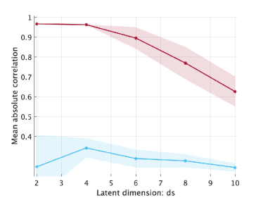
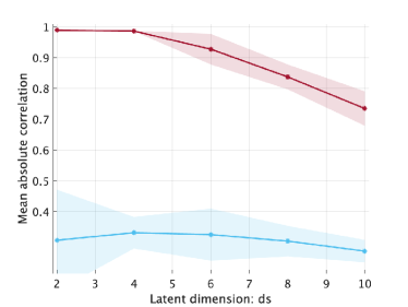
We first present how the performance changes to the latent dimension $d_{\mathrm{s}}$ in Fig.1 when the data dimension and maximum link state are fixed at $d_{\mathrm{x}}=6$ and $K=10$, respectively. GCA (red lines) shows very high correlation values when $d_{\mathrm{s}}$ is less than or equal to $d_{\mathrm{x}}=6$. However, as $d_{\mathrm{s}}$ is more than $d_{\mathrm{x}}=6$, the performance of GCA is quickly decreased. This would be because the mixing function $\bm{f}$ is not bijective in the case of $d_{\mathrm{s}}>d_{\mathrm{x}}$, and cannot be an embedding as assumed in Section 2. On the other hand, EBM (blue lines) shows low correlations on the range of $d_{\mathrm{s}}$. EBM assumes that pairs of $\bm{x}_{i}$ and $\bm{x}_{j}$ are statistically dependent, but $\bm{x}_{1},\dots,\bm{x}_{n}$ are independent in this experiment because $\bm{s}_{1},\dots,\bm{s}_{n}$ are i.i.d. This means that EBM might not be suitable for graph data.

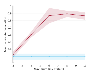
Next, the averages of the mean absolute correlations are presented in Fig.2 when the maximum link state $K$ is modified with $d_{\mathrm{x}}=d_{\mathrm{s}}=6$. Note that EBM does not use link weights, the maximum link weight is fixed at $K=10$ only for learning EBM. When the maximum link state $K$ is less than the latent dimension $d_{\mathrm{s}}=6$, the mean correlations of GCA (red lines) are clearly small. On the other hand, the performance is significantly improved as $K$ is equal to or gets larger than $d_{\mathrm{s}}=6$. This result is fairly consistent, and supports the implication of Corollary 5. Again, since $\bm{x}_{1},\dots,\bm{x}_{n}$ are i.i.d., EBM (blue lines) does not estimate the latent vector $\bm{s}$.

Refer to caption
(a) Independent Laplace
Refer to caption
(b) Correlated Gauss
Figure 1: Mean absolute correlation over the latent dimension $d_{\mathrm{s}}$ when $(d_{\mathrm{x}},K,n)=(6,10,10000)$. The red and blue lines are for GCA and EBM, respectively. Each marker represents the average of the mean absolute correlations over $10$ runs, and the shaded region is the standard deviation.
Refer to caption
(a) Independent Laplace
Refer to caption
(b) Correlated Gauss
Figure 2: Mean absolute correlation over the number of link states when $d_{\mathrm{s}}=d_{\mathrm{x}}$ and $(d_{\mathrm{x}},n)=(6,10000)$. The red and blue lines are for GCA and EBM, respectively. For EBM, the blue line is flat because link weights are not required and the maximum link state is fixed at $K=10$ in learning EBM.

7 Conclusion

This paper proposed a statistical model of two latent vectors with single auxiliary data. Based on the proposed model, we established conditions for partial and full identifiability of the proposed model. Interestingly, the dimensionality relation among latent vectors and auxiliary data would be important conditions for identifiability. When interpreting our model from the reverse data generative process, our work has weak assumptions on the joint and marginal distribution of two latent vectors. In addition, we proved that the indeterminacy of our model has the same indeterminacy as linear ICA under certain conditions. The proposed statistical model and identifiability theory were applied to graph data, and then one of the identifiability conditions includes an interesting implication: The maximum link weight is an important factor for identifiability. Based on the application to graph data, we proposed a practical method for identifiable graph embedding called graph component analysis (GCA). Numerical experiments demonstrated that the performance of GCA clearly depends on the maximum link weight as implied in our theoretical results.

Appendix A Useful lemmas

Our proof is based on the following lemma proved in Sasaki and Takenouchi, (2022):

Lemma 6 (Lemma 10 in Sasaki and Takenouchi, (2022)).

Suppose that $\bm{D}(v)$ is an $n$ by $n$ diagonal matrix whose diagonals $d_{i}(v),i=1\dots,n$ is a function of $v\in\mathbb{R}$, and $\bm{A}$ and $\bm{B}$ are $n$ by $n$ constant matrices. Furthermore, the following assumptions are made:

  1. (1)

    There exist $n$ points $v_{1},v_{2},\dots,v_{n}$ such that $\bm{d}(v_{1}),\bm{d}(v_{2}),\dots,\bm{d}(v_{n})$ are linearly independent where $\bm{d}(v):=(d^{(1)}(v),d^{(2)}(v),\dots,d^{(n)}(v))^{\top}$ is the vector of the diagonal elements in $\bm{D}(v)$.

  2. (2)

    $\bm{A}$ and $\bm{B}$ are of full-rank.

Then, when $\bm{A}\bm{D}(v)\bm{B}$ is a diagonal matrix at least at $n$ points $v_{1},v_{2},\dots,v_{n}$, then both $\bm{A}$ and $\bm{B}$ are diagonal matrices multiplied by a permutation matrix.

We also rely on the following lemma:

Lemma 7.

If $\bm{f}:\mathbb{R}^{d_{\mathrm{s}}}\to\mathbb{R}^{d_{\mathrm{x}}}$ with $d_{\mathrm{s}}\leq{d_{\mathrm{x}}}$ is a smooth embedding, the Jacobian of its inverse $\bm{g}:=\bm{f}^{-1}$ has rank $d_{\mathrm{s}}$.

Proof.

By definition, $\bm{s}=\bm{g}\circ\bm{f}(\bm{s})$. By computing its gradient with respect to $\bm{s}$,

$\displaystyle\bm{I}_{d_{\mathrm{s}}}=\bm{J}_{\bm{g}}(\bm{f}(\bm{s}))^{\top}\bm{J}_{\bm{f}}(\bm{s}).$

Since $\bm{f}$ is a smooth embedding and $\bm{J}_{\bm{f}}(\bm{s})$ has rank $d_{\mathrm{s}}$, the rank of $\bm{J}_{\bm{g}}$ has to be $d_{\mathrm{s}}$. ∎

Appendix B Proof of Theorem 1

Proof.

We first recall that the conditional distribution of $\bm{x}$ and $\bm{u}$ given $\bm{w}$ under $\bm{g}$ and $\bm{\phi}$ is given by

$\displaystyle\log p_{\mathrm{xu}|\mathrm{w}}^{\bm{g},\bm{\phi}}(\bm{x},\bm{u}|\bm{w})$ $\displaystyle=\sum_{i=1}^{d_{\mathrm{s}}}q^{(i)}(g^{(i)}(\bm{x}),\bm{\phi}(\bm{u}),\bm{w})-\log{Z}(\bm{w})$
$\displaystyle\qquad+\frac{1}{2}\log\det(\bm{G}_{\bm{g}}(\bm{x}))+\frac{1}{2}\log\det(\bm{G}_{\bm{\phi}}(\bm{u})).$ (23)

With a single point $\bar{\bm{w}}$ of $\bm{w}$ in Assumption (A3), we have

$\displaystyle\log p_{\mathrm{xu}|\mathrm{w}}^{\bm{g},\bm{\phi}}(\bm{x},\bm{u}|\bm{w})-\log p_{\mathrm{xu}|\mathrm{w}}^{\bm{g},\bm{\phi}}(\bm{x},\bm{u}|\bar{\bm{w}})=\sum_{i=1}^{d_{\mathrm{s}}}{\bar{q}}^{(i)}(g^{(i)}(\bm{x}),\bm{\phi}(\bm{u}),\bm{w})-\log\frac{Z(\bm{w})}{Z(\bar{\bm{w}})},$

where ${\bar{q}}^{(i)}(s,\bm{v},\bm{w}):=q^{(i)}(s,\bm{v},\bm{w})-q^{(i)}(s,\bm{v},\bar{\bm{w}})$. By assuming that the same conditional distribution as (23) exists under $\tilde{\bm{g}}$ and $\tilde{\bm{\phi}}$, we have $p_{\mathrm{xu}|\mathrm{w}}^{\bm{g},\bm{\phi}}(\bm{x},\bm{u}|\bm{w})=p_{\mathrm{xu}|\mathrm{w}}^{\tilde{\bm{g}},\tilde{\bm{\phi}}}(\bm{x},\bm{u}|\bm{w})$ implying

$\displaystyle\sum_{i=1}^{d_{\mathrm{s}}}{\bar{q}}^{(i)}(g^{(i)}(\bm{x}),\bm{\phi}(\bm{u}),\bm{w})=\sum_{i=1}^{d_{\mathrm{s}}}{\bar{q}}^{(i)}(\tilde{g}^{(i)}(\bm{x}),\tilde{\bm{\phi}}(\bm{u}),\bm{w}).$ (24)

Let us express $\tilde{\bm{s}}:=\tilde{\bm{g}}(\bm{x})$ and $\tilde{\bm{v}}:=\tilde{\bm{\phi}}(\bm{u})$, and recall $\bm{s}=\bm{g}(\bm{x})=\bm{g}\circ\tilde{\bm{f}}(\tilde{\bm{s}})$ and $\bm{v}=\bm{\phi}(\bm{u})=\bm{\phi}\circ\tilde{\bm{\varphi}}(\tilde{\bm{v}})$ where $\tilde{\bm{f}}:=\tilde{\bm{g}}^{-1}$ and $\tilde{\bm{\varphi}}:=\tilde{\bm{\phi}}^{-1}$. Then, we express (24) as

$\displaystyle\sum_{i=1}^{d_{\mathrm{s}}}{\bar{q}}^{(i)}(s^{(i)},\bm{v},\bm{w})=\sum_{i=1}^{d_{\mathrm{s}}}{\bar{q}}^{(i)}(\tilde{s}^{(i)},\tilde{\bm{v}},\bm{w}),$ (25)

and then compute the cross-derivative of both sides on (25) with respect to $\tilde{s}^{(l)}$ and $\tilde{s}^{(m)}$ for $l\neq{m}$ as follows:

$\displaystyle\sum_{i=1}^{d}\left\{\frac{\partial^{2}s^{(i)}}{\partial{\tilde{s}^{(l)}}\partial{\tilde{s}^{(m)}}}\bar{q}^{(i,1)}(s^{(i)},\bm{v},\bm{w})+\frac{\partial s^{(i)}}{\partial\tilde{s}^{(l)}}\frac{\partial s^{(i)}}{\partial\tilde{s}^{(m)}}\bar{q}^{(i,2)}(s^{(i)},\bm{v},\bm{w})\right\}=0,$ (26)

where $\bar{q}^{(i,1)}(s,\bm{v},\bm{w}):=\frac{\partial}{\partial{s}}\bar{q}^{(i)}(s,\bm{v},\bm{w})$ and $\bar{q}^{(i,2)}(s,\bm{v},\bm{w}):=\frac{\partial^{2}}{\partial{s^{2}}}\bar{q}^{(i)}(s,\bm{v},\bm{w})$. We further compactly express (26) as the following vector form:

$\displaystyle\bm{a}_{l,m}(\tilde{\bm{s}})^{\top}\bar{\bm{q}}^{\prime}(\bm{s},\bm{v},\bm{w})=0,$ (27)

where

$\displaystyle\bm{a}_{l,m}(\tilde{\bm{s}})$ $\displaystyle:=\left(\frac{\partial^{2}s^{(1)}}{\partial{\tilde{s}^{(l)}}\partial{\tilde{s}^{(m)}}},\dots,\frac{\partial^{2}s^{(d_{\mathrm{s}})}}{\partial{\tilde{s}^{(l)}}\partial{\tilde{s}^{(m)}}},\frac{\partial s^{(1)}}{\partial\tilde{s}^{(l)}}\frac{\partial s^{(1)}}{\partial\tilde{s}^{(m)}},\dots,\frac{\partial s^{(d_{\mathrm{s}})}}{\partial\tilde{s}^{(l)}}\frac{\partial s^{(d_{\mathrm{s}})}}{\partial\tilde{s}^{(m)}}\right)^{\top}\in\mathbb{R}^{2d_{\mathrm{s}}}$
$\displaystyle\bar{\bm{q}}^{\prime}(\bm{s},\bm{v},\bm{w})$ $\displaystyle:=\left(\bar{q}^{(1,1)}(s^{(1)},\bm{v},\bm{w}),\dots,\bar{q}^{(d_{\mathrm{s}},1)}(s^{(d_{\mathrm{s}})},\bm{v},\bm{w}),\right.$
$\displaystyle\left.\qquad\qquad\qquad\qquad\bar{q}^{(1,2)}(s^{(1)},\bm{v},\bm{w}),\dots,\bar{q}^{(d_{\mathrm{s}},2)}(s^{(d_{\mathrm{s}})},\bm{v},\bm{w})\right)^{\top}\in\mathbb{R}^{2d_{\mathrm{s}}}.$

Next, we define the following two vectors where the $i$-th elements in $\bm{v}$ and $\bm{w}$ are fixed:

𝒗(i)superscript𝒗𝑖\displaystyle\bm{v}^{(i)} =(v(1),,v(i)=v¯(i),v(dv))\displaystyle=(v^{(1)},\dots,v^{(i)}=\bar{v}^{(i)}\dots,v^{(d_{\mathrm{v}})})^{\top}
$\displaystyle\bm{w}^{(i)}$ $\displaystyle=(w^{(1)},\dots,w^{(i)}=\bar{w}^{(i)}\dots,w^{(d_{\mathrm{w}})})^{\top}$

These two vectors enable us to express (27) as

$\displaystyle\bm{a}_{l,m}(\tilde{\bm{s}})^{\top}\bar{\bm{Q}}^{\prime}(\bm{s})=\bm{0},$

where

$\displaystyle\bar{\bm{Q}}^{\prime}(\bm{s})$ $\displaystyle:=\left[\bar{\bm{q}}^{\prime}(\bm{s},\bm{v}^{(1)},\bm{w}),\dots,\bar{\bm{q}}^{\prime}(\bm{s},\bm{v}^{(d_{\mathrm{v}})},\bm{w}),\right.$
$\displaystyle\left.\qquad\qquad\bar{\bm{q}}^{\prime}(\bm{s},\bm{v},\bm{w}^{(1)}),\dots,\bar{\bm{q}}^{\prime}(\bm{s},\bm{v},\bm{w}^{(d_{\mathrm{w}})})\right]\biggr{|}_{\bm{v}=\bm{v}^{\prime},\bm{w}=\bm{w}^{\prime}}\in\mathbb{R}^{2d_{\mathrm{s}}\times{(d_{\mathrm{v}}+d_{\mathrm{w}})}}.$

By Assumptions (A2-3), the right inverse of $\bar{\bm{Q}}^{\prime}(\bm{s})$ exists and thus $\bm{a}_{l,m}(\tilde{\bm{s}})=\bm{0}$, i.e.,

$\displaystyle\frac{\partial s^{(i)}}{\partial\tilde{s}^{(l)}}\frac{\partial s^{(i)}}{\partial\tilde{s}^{(m)}}=0,$ (28)

for all $i$ and $(l,m)$ for $l\neq{m}$.

Finally, we complete the proof by showing the Jacobian of $\bm{s}$ with respect to $\tilde{\bm{s}}$ is of full rank. With $\bm{s}=\bm{g}\circ\tilde{\bm{f}}(\tilde{\bm{s}})$,

$\displaystyle\bm{J}_{\bm{s}}(\tilde{\bm{s}})=\bm{J}_{\bm{g}}(\tilde{\bm{f}}(\tilde{\bm{s}}))^{\top}\bm{J}_{\tilde{\bm{f}}}(\tilde{\bm{s}}).$

Since $\tilde{\bm{f}}$ is a smooth embedding, $\bm{J}_{\tilde{\bm{f}}}$ has rank $d_{\mathrm{s}}$, and Lemma 7 ensures that $\bm{J}_{\bm{g}}$ also has rank $d_{\mathrm{s}}$. Thus, $\bm{J}_{\bm{s}}(\tilde{\bm{s}})$ has $d_{\mathrm{s}}$ rank and is of full rank. Thus, by (28), each row of $\bm{J}_{\bm{s}}(\tilde{\bm{s}})$ has a single nonzero element. This means that each $s_{i}$ is a function of a single variable in $\tilde{\bm{s}}$, which completes the proof. ∎

Appendix C Proof of Theorem 2

Proof.

We begin by differentiating (25) with respect to $s^{(l)}$ and $v^{m}$ as

$\displaystyle\bar{q}_{\mathrm{w}}^{(l)}(\bm{w})\frac{\partial^{2}}{\partial s^{(l)}\partial{v}^{(m)}}q_{\mathrm{sv}}^{(l)}(s^{(l)},\bm{v})$
$\displaystyle\quad=\sum_{i=1}^{d_{\mathrm{s}}}\sum_{j=1}^{d_{\mathrm{v}}}\bar{q}_{\mathrm{w}}^{(i)}(\bm{w})\frac{\partial\tilde{s}^{(i)}}{\partial s^{(l)}}\frac{\partial\tilde{v}^{(j)}}{\partial v^{(m)}}\frac{\partial^{2}}{\partial\tilde{s}^{(i)}\partial{\tilde{v}}^{(j)}}q_{\mathrm{sv}}^{(i)}(\tilde{s}^{(i)},\tilde{\bm{v}}),$ (29)

where Assumption (B1) was applied. Eq.(29) can be expressed as the following matrix form:

$\displaystyle\bm{D}(\bm{w})\bm{Q}_{\mathrm{sv}}(\bm{s},\bm{v})=\bm{J}_{\tilde{\bm{s}}}(\bm{s})^{\top}\bm{D}(\bm{w})\bm{Q}_{\mathrm{sv}}(\tilde{\bm{s}},\tilde{\bm{v}})\bm{J}_{\tilde{\bm{v}}}(\bm{v}),$ (30)

where $\bm{D}(\bm{w}):=\mathrm{diag}(\bar{q}_{\mathrm{w}}^{(d_{\mathrm{s}})}(\bm{w}),\dots,\bar{q}_{\mathrm{w}}^{(d_{\mathrm{s}})}(\bm{w}))$ and $\bm{Q}_{\mathrm{sv}}(\bm{s},\bm{v})$ is a $d_{\mathrm{s}}$ by $d_{\mathrm{v}}$ matrix with the $(l,m)$-th element $\frac{\partial^{2}}{\partial{s}^{(l)}\partial{v}^{(m)}}q_{\mathrm{sv}}^{(l)}(s^{(l)},\bm{v})$. By Assumptions (B2-3), $\bm{Q}_{\mathrm{sv}}(\bm{s},\bm{v}=\bm{v}^{\prime})$ has the right inverse. Thus, by denoting the right inverse by $\bm{Q}_{\mathrm{sv}}^{\dagger}(\bm{s})$, we have from (30),

$\displaystyle\bm{D}(\bm{w})=\bm{J}_{\tilde{\bm{s}}}(\bm{s})^{\top}\bm{D}(\bm{w})\underbrace{\bm{Q}_{\mathrm{sv}}(\tilde{\bm{s}},\tilde{\bm{v}}^{\prime})\bm{J}_{\tilde{\bm{v}}}(\bm{v}^{\prime})\bm{Q}_{\mathrm{sv}}^{\dagger}(\bm{s})}_{\bm{M}(\bm{s})},$ (31)

where $\tilde{\bm{v}}^{\prime}:=\tilde{\bm{\phi}}\circ\bm{\varphi}(\bm{v}^{\prime})$. Assumption (B4) ensures that $\bm{D}(\bm{w})$ is full rank for $\bm{w}\in\{\bm{w}(1),\dots,\bm{w}(d_{\mathrm{s}})\}$. In addition, $\bm{J}_{\tilde{\bm{s}}}(\bm{s})$ has also full rank because $\bm{f}$ is a smooth embedding. Thus, $\bm{M}(\bm{s})\in\mathbb{R}^{d_{\mathrm{s}}\times{d_{\mathrm{s}}}}$ must be of full rank. By Assumption (B4), the vectors of the diagonals in $\bm{D}(\bm{w})$ for $\bm{w}\in\{\bm{w}(1),\dots,\bm{w}(d_{\mathrm{s}})\}$ are linearly independent. Therefore, applying Lemma 6 to (31) indicates that $\bm{J}_{\tilde{\bm{s}}}(\bm{s})$ is the product of a diagonal and permutation matrix. This completes the proof. ∎

Appendix D Proof of Theorem 3

Proof.

We first compute the partial derivative of (25) with respect to $s^{(l)}$ and $v^{(m)}$ under Assumption (C1) as

$\displaystyle\frac{\partial^{2}}{\partial{s}^{(l)}\partial{v^{(m)}}}\bar{q}^{(l)}(s^{(l)},v^{(m)},\bm{w})=\sum_{i=1}^{d}\frac{\partial\tilde{s}^{(i)}}{\partial s^{(l)}}\frac{\partial\tilde{v}^{(i)}}{\partial v^{(m)}}\frac{\partial^{2}}{\partial{\tilde{s}^{(i)}}\partial{\tilde{v}^{(i)}}}\bar{q}^{(i)}(\tilde{s}^{(i)},\tilde{v}^{(i)},\bm{w}).$ (32)

We further compactly express (32) in a matrix form as

$\displaystyle\bm{D}(\bm{s},\bm{v},\bm{w})=(\bm{J}_{\tilde{\bm{s}}}(\bm{s}))^{\top}\bm{D}(\bm{w},\tilde{\bm{s}},\tilde{\bm{v}})\bm{J}_{\tilde{\bm{v}}}(\bm{v}),$ (33)

where $\bm{D}(\bm{s},\bm{v},\bm{w})$ is a diagonal matrix with the $i$-th diagonal $\frac{\partial^{2}}{\partial{s}^{(i)}\partial{v^{(i)}}}\bar{q}^{(i)}(s^{(i)},v^{(i)},\bm{w})$.

As in previous proofs, our goal is to show that $\bm{J}_{\tilde{\bm{s}}}(\bm{s})$ is the product of a permutation and diagonal matrix. To this end, we substitute $\bm{v}^{\prime}$ into $\bm{v}$ in (33) and have

$\displaystyle\bm{D}_{\mathrm{v^{\prime}}}(\bm{s},\bm{w})$ $\displaystyle=(\bm{J}_{\tilde{\bm{s}}}(\bm{s}))^{\top}\bm{D}_{\mathrm{\tilde{v}^{\prime}}}(\tilde{\bm{s}},\bm{w})\bm{J}^{\prime}_{\tilde{\bm{v}}},$ (34)

where $\bm{D}_{\mathrm{v^{\prime}}}(\bm{s},\bm{w}):=\bm{D}(\bm{s},\bm{v}^{\prime},\bm{w})$, $\bm{D}_{\mathrm{\tilde{v}^{\prime}}}(\bm{s},\bm{w}):=\bm{D}(\bm{s},\tilde{\bm{v}}=\tilde{\bm{\phi}}\circ\bm{\varphi}(\bm{v}^{\prime}),\bm{w})$ and $\bm{J}^{\prime}_{\tilde{\bm{v}}}:=\bm{J}_{\tilde{\bm{v}}}(\bm{v}^{\prime})$. Since $\bm{\varphi}$ is a smooth embedding, $\bm{J}^{\prime}_{\tilde{\bm{v}}}$ is of full rank. Furthermore, Assumption (C2) ensures that $\bm{D}_{\mathrm{v^{\prime}}}(\bm{s},\bm{w})$ is of full-rank for $\bm{w}\in\{\bm{w}(1),\dots,\bm{w}(d_{\mathrm{s}})\}$ and all $\bm{s}$. Thus, for each $\bm{s}$ as well as $\tilde{\bm{s}}=\tilde{\bm{g}}\circ{\bm{f}}(\bm{s})$, applying Lemma 6 to the right-hand side on (34) under Assumption (C2) indicates that both $\bm{J}_{\tilde{\bm{s}}}(\bm{s})$ and $\bm{J}^{\prime}_{\tilde{\bm{v}}}$ are the product of diagonal and permutation matrix. The proof is completed. ∎

Appendix E Proof of Proposition 4

Proof.

Here, some notations are inherited from Appendix D. From (13), we have

$\displaystyle\frac{\partial^{2}}{\partial{s^{(i)}}\partial{v^{(i)}}}\bar{q}^{(i)}(\bm{w},s_{i},v_{i})$ $\displaystyle=\alpha^{(i)}(\bm{w},v^{(i)})$
$\displaystyle\frac{\partial^{2}}{\partial{\tilde{s}^{(i)}}\partial{\tilde{v}^{(i)}}}\bar{q}^{(i)}(\bm{w},\tilde{s}_{i},\tilde{v}^{(i)})$ $\displaystyle=\alpha^{(i)}(\bm{w},\tilde{v}^{(i)}).$

Thus, once $\bm{w}$ is fixed at $\bm{w}=\bm{w}^{\prime}$, both $\bm{D}_{\mathrm{v^{\prime}}}(\bm{s},\bm{w}=\bm{w}^{\prime})$ and $\bm{D}_{\mathrm{\tilde{v}^{\prime}}}(\tilde{\bm{s}},\bm{w}=\bm{w}^{\prime})$ in (33) are constant diagonal matrices whose diagonals are given by $(\alpha^{(1)}(\bm{w},v^{(1)}),\dots,\alpha^{(d)}(\bm{w},v^{(d)}))|_{\bm{w}=\bm{w}^{\prime},\bm{v}=\bm{v}^{\prime}}$ and $(\alpha^{(1)}(\bm{w},\tilde{v}^{(1)}),\dots,\alpha^{(d)}(\bm{w},\tilde{v}^{(d)}))|_{\bm{w}=\bm{w}^{\prime},\tilde{\bm{v}}=\tilde{\bm{\phi}}\circ\bm{\varphi}(\bm{v}^{\prime})}$, respectively. Thus, we re-express these matrices simply by $\bm{D}_{\mathrm{w^{\prime}v^{\prime}}}$ and $\bm{D}_{\mathrm{w^{\prime}\tilde{v}^{\prime}}}$. Then, it follows from (34) that $\bm{J}_{\tilde{\bm{s}}}(\bm{s})$ can be expressed as

$\displaystyle\bm{J}_{\tilde{\bm{s}}}(\bm{s})=(\bm{D}_{\mathrm{w^{\prime}\tilde{v}^{\prime}}}\bm{J}^{\prime}_{\tilde{\bm{v}}})^{-\top}\bm{D}_{\mathrm{w^{\prime}v^{\prime}}}.$ (35)

As proved in Appendix D, $\bm{J}^{\prime}_{\tilde{\bm{v}}}$ is the product of a diagonal and permutation matrix. Thus, (35) indicates that there exist a nonzero constant $\gamma^{(i)}$ and permutation index $\pi(i)\in\{1,\dots,d_{\mathrm{s}}\}$ such that

$\displaystyle\frac{\partial\tilde{s}^{(i)}}{\partial s^{(\pi(j))}}=\left\{\begin{array}[]{cc}\gamma^{(i)}&i=j\\ 0&i\neq{j}\end{array}\right.$

This completes the proof. ∎

Appendix F Reverse generative model

Here, we give details of why identifiability is guaranteed in the reverse generative model as well. The proofs for all of theorems come with the partial derivatives of (25) or its variants. Thus, it suffices to show (25) holds in the reverse generative model. As an alternative to $p_{\mathrm{sv}|\mathrm{w}}(\bm{s},\bm{v}|\bm{w})$ in Theorem 1, we assume that the conditional distribution of $\bm{w}$ given $\bm{s}$ and $\bm{v}$ is given in the reverse generative model by

$\displaystyle\log p_{\mathrm{w}|\mathrm{sv}}(\bm{w}|\bm{s},\bm{v})=\sum_{i=1}^{d_{\mathrm{s}}}q^{(i)}(s^{(i)},\bm{v},\bm{w})-\log{Z}(\bm{s},\bm{v}).$

Then, by $\bm{s}=\bm{g}(\bm{x})$ and $\bm{v}=\bm{\phi}(\bm{u})$, we obtain the conditional distribution of $\bm{w}$ given $\bm{x}$ and $\bm{u}$ as

$\displaystyle\log p_{\mathrm{w}|\mathrm{xu}}^{\bm{g},\bm{\phi}}(\bm{w}|\bm{x},\bm{u})=\sum_{i=1}^{d_{\mathrm{s}}}q^{(i)}(g^{(i)}(\bm{x}),\bm{\phi}(\bm{u}),\bm{w})-\log{Z}(\bm{x},\bm{u}).$

With a single point $\bar{\bm{w}}$ of $\bm{w}$ in Assumption (A3), we have

$\displaystyle\log p_{\mathrm{w}|\mathrm{xu}}^{\bm{g},\bm{\phi}}(\bm{w}|\bm{x},\bm{u})-\log p_{\mathrm{xu}|\mathrm{w}}^{\bm{g},\bm{\phi}}(\bar{\bm{w}}|\bm{x},\bm{u})=\sum_{i=1}^{d_{\mathrm{s}}}{\bar{q}}^{(i)}(g^{(i)}(\bm{x}),\bm{\phi}(\bm{u}),\bm{w}).$

Finally, $p_{\mathrm{xu}|\mathrm{w}}^{\bm{g},\bm{\phi}}(\bm{x},\bm{u}|\bm{w})=p_{\mathrm{xu}|\mathrm{w}}^{\tilde{\bm{g}},\tilde{\bm{\phi}}}(\bm{x},\bm{u}|\bm{w})$ enables us to obtain (25). By exactly following the steps after (25), we reach the same conclusion as Theorem 1 if the other assumptions are retained. It can be shown in the reverse generative model that the conclusions of Theorems 2 and 3 hold in the same way above.

Appendix G Learning energy-based models

This appendix gives details for learning energy-based models in Section 6. Here, we take a similar approach as GCA and estimate the following density ratio:

$\displaystyle\frac{p_{\mathrm{x|x^{\prime}}}(\bm{x}|\bm{x}^{\prime})}{p_{\mathrm{x}}(\bm{x})}.$

To estimate it, the objective function based on the Donsker-Varadhan variational estimation is used as

$\displaystyle J_{\mathrm{DV}}(r)$ $\displaystyle:=-\iint{r}(\bm{x},\bm{x}^{\prime})p_{\mathrm{xx^{\prime}}}(\bm{x},\bm{x}^{\prime})\mathrm{d}\bm{x}\mathrm{d}\bm{x}^{\prime}$
$\displaystyle\qquad\qquad+\log\left(\iint e^{r(\bm{x},\bm{x}^{\prime})}p_{\mathrm{x}}(\bm{x})p_{\mathrm{x}}(\bm{x}^{\prime})\mathrm{d}\bm{x}\mathrm{d}\bm{x}^{\prime}\right).$ (36)

A simple calculation shows that $J_{\mathrm{DV}}(r)$ is minimized at the following distribution ratio:

$\displaystyle r(\bm{x},\bm{x}^{\prime})=\log p_{\mathrm{x|x^{\prime}}}(\bm{x}|\bm{x}^{\prime})-\log p_{\mathrm{x}}(\bm{x})$

Thus, $r(\bm{x},\bm{x}^{\prime})$ is modeled as

$\displaystyle r(\bm{x},\bm{x}^{\prime})=\bm{h}(\bm{x})^{\top}\bm{h}(\bm{x}^{\prime})+a(\bm{h}(\bm{x})),$

where $a(\cdot)$ is modeled as a single layer neural network without activation function. Then, we empirically approximate $J_{\mathrm{DV}}(r)$ from data samples as follows:

$\displaystyle\widehat{J}_{\mathrm{DV}}(r)$ $\displaystyle:=-\frac{1}{|\mathcal{I}_{n}|}\sum_{(i,j)\in\mathcal{I}_{n}}r(\bm{x}_{i},\bm{x}_{j})+\log\left(\frac{1}{|\mathcal{I}_{n}|}\sum_{(i,j)\in\mathcal{I}_{n}}e^{r(\bm{x}_{i},\bm{x}^{*}_{j})}\right),$ (37)

where $\bm{x}^{*}_{j}$ is a random permutation of $\bm{x}^{*}_{j}$ with respect to $j$. Learning EBM is completed by minimizing $\widehat{J}_{\mathrm{DV}}(r)$.

References

  • Belghazi et al., (2018) Belghazi, M., Baratin, A., Rajeshwar, S., Ozair, S., Bengio, Y., Hjelm, D., and Courville, A. (2018). Mutual information neural estimation. In Proceedings of the 35th International Conference on Machine Learning (ICML), volume 80, pages 530–539.
  • Bengio et al., (2013) Bengio, Y., Courville, A., and Vincent, P. (2013). Representation learning: A review and new perspectives. IEEE Transactions on Pattern Analysis and Machine Intelligence, 35(8):1798–1828.
  • Buchholz et al., (2022) Buchholz, S., Besserve, M., and Schölkopf, B. (2022). Function classes for identifiable nonlinear independent component analysis. Advances in Neural Information Processing Systems (NeurIPS), 35:16946–16961.
  • Cai et al., (2018) Cai, H., Zheng, V. W., and Chang, K. C.-C. (2018). A comprehensive survey of graph embedding: Problems, techniques, and applications. IEEE Transactions on Knowledge and Data Engineering, 30(9):1616–1637.
  • Comon, (1994) Comon, P. (1994). Independent component analysis, a new concept? Signal Processing, 36(3):287–314.
  • Devlin et al., (2019) Devlin, J., Chang, M.-W., Lee, K., and Toutanova, K. (2019). BERT: Pre-training of deep bidirectional transformers for language understanding. In Proceedings of the 2019 Conference of the North American Chapter of the Association for Computational Linguistics: Human Language Technologies, pages 4171–4186.
  • Gemici et al., (2016) Gemici, M. C., Rezende, D., and Mohamed, S. (2016). Normalizing flows on Riemannian manifolds. arXiv preprint arXiv:1611.02304.
  • Gresele et al., (2019) Gresele, L., Rubenstein, P., Mehrjou, A., Locatello, F., and Schölkopf, B. (2019). The incomplete Rosetta Stone problem: Identifiability results for multi-view nonlinear ICA. In Proceedings of the 35th International Conference on Uncertainty in Artificial Intelligence (UAI), pages 296–313.
  • Gresele et al., (2021) Gresele, L., Von Kügelgen, J., Stimper, V., Schölkopf, B., and Besserve, M. (2021). Independent mechanism analysis, a new concept? Advances in neural information processing systems (NeurIPS), 34:28233–28248.
  • Gutmann and Hyvärinen, (2012) Gutmann, M. and Hyvärinen, A. (2012). Noise-contrastive estimation of unnormalized statistical models, with applications to natural image statistics. Journal of Machine Learning Research, 13:307–361.
  • Gutmann and Hirayama, (2011) Gutmann, M. U. and Hirayama, J. (2011). Bregman divergence as general framework to estimate unnormalized statistical models. In Proceedings of the Twenty-Seventh Conference on Uncertainty in Artificial Intelligence (UAI), pages 283–290.
  • Hälvä et al., (2021) Hälvä, H., Le Corff, S., Lehéricy, L., So, J., Zhu, Y., Gassiat, E., and Hyvarinen, A. (2021). Disentangling identifiable features from noisy data with structured nonlinear ICA. In Advances in Neural Information Processing Systems (NeurIPS), volume 34, pages 1624–1633.
  • Hyvärinen and Morioka, (2016) Hyvärinen, A. and Morioka, H. (2016). Unsupervised feature extraction by time-contrastive learning and nonlinear ICA. In Advances in Neural Information Processing Systems (NeurIPS), pages 3765–3773.
  • Hyvärinen and Morioka, (2017) Hyvärinen, A. and Morioka, H. (2017). Nonlinear ICA of temporally dependent stationary sources. In Proceedings of the 20th International Conference on Artificial Intelligence and Statistics (AISTATS), volume 54, pages 460–469. PMLR.
  • Hyvärinen and Pajunen, (1999) Hyvärinen, A. and Pajunen, P. (1999). Nonlinear independent component analysis: Existence and uniqueness results. Neural Networks, 12(3):429–439.
  • Hyvärinen et al., (2019) Hyvärinen, A., Sasaki, H., and Turner, R. E. (2019). Nonlinear ICA using auxiliary variables and generalized contrastive learning. In Proceedings of the 22th International Conference on Artificial Intelligence and Statistics (AISTATS), volume 89, pages 859–868.
  • (17) Khemakhem, I., Kingma, D. P., Monti, R. P., and Hyvärinen, A. (2020a). Variational autoencoders and nonlinear ICA: A unifying framework. In Proceedings of the Twenty Third International Conference on Artificial Intelligence and Statistics (AISTATS), volume 108, pages 2207–2217. PMLR.
  • (18) Khemakhem, I., Monti, R., Kingma, D., and Hyvarinen, A. (2020b). ICE-BeeM: Identifiable conditional energy-based deep models based on nonlinear ICA. Advances in Neural Information Processing Systems (NeurIPS), 33:12768–12778.
  • Kingma and Ba, (2015) Kingma, D. P. and Ba, J. (2015). Adam: A method for stochastic optimization. In Proceedings of the 3rd International Conference on Learning Representations (ICLR), pages 1–15.
  • Klindt et al., (2020) Klindt, D. A., Schott, L., Sharma, Y., Ustyuzhaninov, I., Brendel, W., Bethge, M., and Paiton, D. (2020). Towards nonlinear disentanglement in natural data with temporal sparse coding. In International Conference on Learning Representations (ICLR).
  • Lee, (2012) Lee, J. (2012). Introduction to Smooth Manifolds. Springer.
  • Locatello et al., (2019) Locatello, F., Bauer, S., Lucic, M., Raetsch, G., Gelly, S., Schölkopf, B., and Bachem, O. (2019). Challenging common assumptions in the unsupervised learning of disentangled representations. In Proceedings of the 36th International Conference on Machine Learning (ICML), volume 97 of Proceedings of Machine Learning Research, pages 4114–4124. PMLR.
  • Locatello et al., (2020) Locatello, F., Poole, B., Rätsch, G., Schölkopf, B., Bachem, O., and Tschannen, M. (2020). Weakly-supervised disentanglement without compromises. In International Conference on Machine Learning (ICML), pages 6348–6359. PMLR.
  • Lyu et al., (2022) Lyu, Q., Fu, X., Wang, W., and Lu, S. (2022). Understanding latent correlation-based multiview learning and self-supervision: An identifiability perspective. In International Conference on Learning Representations (ICLR).
  • Monti et al., (2020) Monti, R. P., Zhang, K., and Hyvärinen, A. (2020). Causal discovery with general non-linear relationships using non-linear ICA. In Proceedings of the 35th Conference on Uncertainty in Artificial Intelligence (UAI), pages 186–195.
  • Okuno et al., (2018) Okuno, A., Hada, T., and Shimodaira, H. (2018). A probabilistic framework for multi-view feature learning with many-to-many associations via neural networks. In Proceedings of the 35th International Conference on Machine Learning (ICML), volume 80 of Proceedings of Machine Learning Research, pages 3888–3897. PMLR.
  • Okuno and Shimodaira, (2019) Okuno, A. and Shimodaira, H. (2019). Robust graph embedding with noisy link weights. In Proceedings of the 22nd International Conference on Artificial Intelligence and Statistics (AISTATS), pages 664–673. PMLR.
  • Peters et al., (2018) Peters, M., Neumann, M., Iyyer, M., Gardner, M., Clark, C., Lee, K., and Zettlemoyer, L. (2018). Deep contextualized word representations. In Proceedings of the 2018 Conference of the North American Chapter of the Association for Computational Linguistics: Human Language Technologies, pages 2227–2237.
  • Raina et al., (2007) Raina, R., Battle, A., Lee, H., Packer, B., and Ng, A. Y. (2007). Self-taught learning: transfer learning from unlabeled data. In Proceedings of the 24th International Conference on Machine Learning (ICML), pages 759–766.
  • Ruderman et al., (2012) Ruderman, A., Reid, M. D., García-García, D., and Petterson, J. (2012). Tighter variational representations of $f$-divergences via restriction to probability measures. In Proceedings of the 29th International Conference on Machine Learning (ICML), pages 1155–1162.
  • Sasaki and Hyvärinen, (2018) Sasaki, H. and Hyvärinen, A. (2018). Neural-kernelized conditional density estimation. arXiv preprint arXiv:1806.01754.
  • Sasaki and Takenouchi, (2022) Sasaki, H. and Takenouchi, T. (2022). Representation learning for maximization of mi, nonlinear ica and nonlinear subspaces with robust density ratio estimation. Journal of Machine Learning Research, 23(231):1–55.
  • Satta and Sasaki, (2022) Satta, K. and Sasaki, H. (2022). Graph embedding with outlier-robust ratio estimation. IEICE Transactions on Information and Systems, 105(10):1812–1816.
  • Teshima et al., (2020) Teshima, T., Sato, I., and Sugiyama, M. (2020). Few-shot domain adaptation by causal mechanism transfer. In Proceedings of the 37th International Conference on Machine Learning (ICML), volume 119, pages 9458–9469.
  • Uehara et al., (2020) Uehara, M., Kanamori, T., Takenouchi, T., and Matsuda, T. (2020). A unified statistically efficient estimation framework for unnormalized models. In International Conference on Artificial Intelligence and Statistics (AISTATS), pages 809–819. PMLR.
  • Wu and Fukumizu, (2020) Wu, P. and Fukumizu, K. (2020). Causal mosaic: Cause-effect inference via nonlinear ICA and ensemble method. In Proceedings of the Twenty Third International Conference on Artificial Intelligence and Statistics (AISTATS), volume 108, pages 1157–1167.
  • Zheng et al., (2022) Zheng, Y., Ng, I., and Zhang, K. (2022). On the identifiability of nonlinear ICA: Sparsity and beyond. Advances in Neural Information Processing Systems (NeurIPS), 35:16411–16422.