Do spectral cues matter in contrast-based graph self-supervised learning?

Abstract

The recent surge in contrast-based graph self-supervised learning has prominently featured an intensified exploration of spectral cues. However, an intriguing paradox emerges, as methods grounded in seemingly conflicting assumptions or heuristic approaches regarding the spectral domain demonstrate notable enhancements in learning performance. This paradox prompts a critical inquiry into the genuine contribution of spectral information to contrast-based graph self-supervised learning. This study undertakes an extensive investigation into this inquiry, conducting a thorough study of the relationship between spectral characteristics and the learning outcomes of contemporary methodologies. Based on this analysis, we claim that the effectiveness and significance of spectral information need to be questioned. Instead, we revisit simple edge perturbation: random edge dropping designed for node-level self-supervised learning and random edge adding intended for graph-level self-supervised learning. Compelling evidence is presented that these simple yet effective strategies consistently yield superior performance while demanding significantly fewer computational resources compared to all prior spectral augmentation methods. The proposed insights represent a significant leap forward in the field, potentially reshaping the understanding and implementation of graph self-supervised learning.

1 Introduction

In recent years, graph learning has emerged as a powerhouse for handling complex data relationships in multiple fields, offering vast potential and value, particularly in domains such as data mining [10], computer vision [35], network analysis [4], and bioinformatics [12]. However, limited labels make graph learning challenging to apply in real-world scenarios. Inspired by the great success of Self-Supervised Learning (SSL) in other domains [6, 3], Graph Self-Supervised Learning (Graph SSL) has made rapid progress and has shown promise by achieving state-of-the-art performance on many tasks [34], where Contrast-based Graph SSL (CG-SSL) are most dominate [20]. This type of method is grounded in the concept of mutual information (MI) maximization. The primary goal is to maximize the estimated MI between augmented instances of the same object, such as nodes, subgraphs, or entire graphs. Among the new developments in CG-SSL, approaches inspired by graph spectral methods have garnered significant attention. A prevalent conviction is that spectral information, including the eigenvalues and eigenvectors of the graph’s Laplacian, plays a crucial role in enhancing the efficacy of CG-SSL [18, 14, 16, 36].

Several methodologies heavily emphasize the utilization of spectral information while implementing sampling or sparsification procedures to enhance learning capabilities. However, there seems no consensus on the effectiveness of spectral information can be made. SpCo [18] introduces the general graph augmentation (GAME) rule, which suggests that the difference in high-frequency parts between augmented graphs should be larger than that of low-frequency parts. SPAN [16] contends that effective topology augmentation in Graph Contrastive Learning (GCL) should prioritize perturbing sensitive edges that have a substantial impact on the graph spectrum. Therefore, a principled augmentation method is designed by directly maximizing spectral change with a certain perturbation budget. GASSER [36] selectively perturbs graph structures based on spectral cues to better maintain the required invariance for contrastive learning frameworks. A contradiction emerges among these related works on spectral augmentation: SPAN advocates for maximizing the disparity between augmented graphs, while SpCo and GASSER argue for the preservation of specific spectral components during augmentation. Moreover, SpCo underscores the task-agnostic significance of retaining information from low-frequency components, whereas GASSER suggests that augmentations should selectively preserve task-relevant frequency components while cautiously perturbing task-irrelevant ones. The consistent performance gain derived from opposing methodical designs naturally raises our concern:

•  Does spectral cues really matter in contrast-based graph SSL?

Given the question, this study aims to critically evaluate the effectiveness and significance of spectral augmentation in contrast-based graph SSL frameworks (CG-SSL). With evidence-supported claims and findings in the following sections, we can give a negative answer to the question above: No, they are not very effective and we don’t really need them. To be specific, we find that spectral augmentation does not significantly contribute to the learning efficacy while more straightforward edge perturbations are already good enough for contrast-based graph SSL. We manage to elaborate on our conclusion through a series of studies carried out in the following efforts:

1. In Sec. 4, we explore the dependency of spectral augmentation effectiveness on the depth of the network, positing that shallower networks with fewer convolutional layers perform better but demonstrate diminished benefits from spectral changes.

2. In Sec 5 We claim that simple edge perturbation techniques, like adding edges to or dropping edges from the graph, not only compete well but often outperform spectral augmentations, without any significant help from spectral cues. To support this,

   (a) In Sec. 6, overall model performance on test accuracy with four state-of-the-art frameworks on both node- and graph-level classification tasks support the superiority of simple edge perturbation. (b) Studies in Sec. 7.1 reveal the indistinguishability between the average spectrum of augmented graphs from edge perturbation with optimal parameters on different datasets, no matter how different that of original graphs is, indicating GNN encoders can hardly learn spectral information from augmented graphs. That is to say, edge perturbations can not benefit from spectral cues. (c) In Sec. 7.2, we analyze the effectiveness of state-of-the-art spectral augmentation baseline (i.e., SPAN) by perturbing edges to alter the spectral characteristics of augmented graphs from simple edge perturbation augmentation and examining the impact on model performance. As it turns out, the results show no performance degradation, indicating the spectral information contained in the augmentation is not significant to the model performance. (d) In Appendix E.2, statistical analysis is carried out to argue that the major reason edge perturbation works well is not because of the spectral information as they are not the key factor on model performance.

2 Related work

Graph Contrastive Learning. Contrast-based Graph Self-Supervised (CG-SSL) learning alleviates the limitations of supervised learning, which heavily depends on labeled data and often suffers from limited generalization [19]. This makes it a promising approach for real-world applications where labeled data is scarce. In general, CG-SSL can be categorized into Graph Contrastive Learning (GCL) and Graph Predictive Learning [34], here we focus our discussion on the former. GCL applies a variety of augmentations to the training graph to obtain augmented views. These augmented views, which are derived from the same original graph, are treated as positive sample pairs or sets. The key objective of GCL is to maximize the mutual information between these views to learn robust and invariant representations. However, directly computing the mutual information of graph representations is challenging. Hence, in practice, GCL frameworks aim to maximize the lower bound of mutual information using different estimators such as InfoNCE [9], Jensen-Shannon [22], and Donsker-Varadhan [1]. For instance, frameworks like GRACE [42], GCC [25], and GCA [43] utilize the InfoNCE estimator as their objective function. On the other hand, MVGRL [11] and InfoGraph [28] adopt the Jensen-Shannon estimator.

Graph Augmentations in GCL. Beyond the choice of object functions, another crucial aspect of GCL is the selection of augmentation techniques. Early work by [42] and [37] introduced several heuristic domain-agnostic graph augmentation for CG-SSL, such as edge perturbation, attribute masking, and subgraph sampling. These straightforward and effective methods have been widely adopted in subsequent CG-SSL frameworks due to their demonstrated success [29, 38]. However, these domain-agnostic graph augmentations often lack interpretability, making it difficult to understand the exact impact of these augmentations on the graph structure and learning outcomes. To address this issue, MVGRL [11] introduces graph diffusion as an augmentation strategy, where the original graph provides local structural information and the diffused graph offers global context. MVGRL demonstrates experimentally that by optimizing for consistency between node representations from these two perspectives, it’s possible to obtain representations that encode both local and global structural information. Moreover, SpCo [18], GASSER [36], and SPAN [16] provide design principles for graph augmentation based on spectral graph theory, further elaborating on how graph augmentation can help CG-SSL. However, our explorations show that these methods are unable to consistently outperform heuristic graph augmentations such as edge perturbation (DropEdge or AddEdge) in terms of performance under fair comparisons, and thus the design principles of graph augmentation still require further validation.

3 Preliminary study

Contrast-based graph self-supervised learning framework.

CG-SSL captures invariant features of a graph by generating multiple views (typically two) through augmentations and then maximizing the mutual information between these views [34]. This approach is ultimately used to improve performance on various downstream tasks. Following previous work [33, 19, 34], we first denote the generic form of the augmentation $\mathcal{T}$ and objective functions $\mathcal{L}_{cl}$ of graph contrastive learning. Given a graph $\mathcal{G}=(\mathbf{A},\mathbf{X})$ with adjacency matrix $\mathbf{A}$ and feature matrix $\mathbf{X}$, the augmentation is defined as the transformation function $\mathcal{T}$. In this paper, we are mainly concerned with topological augmentation, in which feature matrix $\mathbf{X}$ remains intact:

$$\widetilde{\mathbf{A}},\widetilde{\mathbf{X}}=\mathcal{T}(\mathbf{A},\mathbf{X})=\mathcal{T}(\mathbf{A}),\mathbf{X}$$ (1)

In practice, two augmented views of the graph are generated, denoted as $\mathcal{G}^{(1)}=\mathcal{G}(\mathcal{T}_{1}(\mathbf{A},\mathbf{X}))$ and $\mathcal{G}^{(2)}=\mathcal{G}(\mathcal{T}_{2}(\mathbf{A},\mathbf{X}))$. The objective of GCL is to learn representations by minimizing the contrastive loss $\mathcal{L}_{cl}$ between the augmented views:

$$\theta^{*},\phi^{*}=\underset{\theta,\phi}{\arg\min}\mathcal{L}_{cl}\left(p_{\phi}\left(f_{\theta}\left({\mathcal{G}}^{(1)}\right),f_{\theta}\left({\mathcal{G}}^{(2)}\right)\right)\right),$$ (2)

where $f_{\theta}$ represents the graph encoder parameterized by $\theta$, and $p_{\phi}$ is a projection head parameterized by $\phi$. The goal is to find the optimal parameters $\theta^{*}$ and $\phi^{*}$ that minimize the contrastive loss.

In this paper, we utilize four prominent CG-SSL frameworks to study the effect of spectral: MVGRL, GRACE, BGRL, and G-BT. MVGRL introduces graph diffusion as augmentation, while the other three frameworks use edge perturbation as augmentation. Each framework employs different strategies for its contrastive loss functions. MVGRL and GRACE use the Jensen-Shannon and InfoNCE estimators as object functions, respectively. In contrast, BGRL and G-BT adopt the BYOL loss [7] and Barlow Twins loss [39], which are designed to maximize the agreement between the augmented views without relying on negative samples. A more detailed description of the loss function can be found in the Appendix D.

Graph spectrum and application of spectral augmentation.

We follow the standard definition of graph spectrum in this study, details of which can be found in Appendix C. Among various augmentation strategies proposed to enhance the robustness and generalization of graph neural networks, spectral augmentation has been considered a promising avenue [16, 18, 2, 36]. Spectral augmentation typically involves implicit modifications to the eigenvalues of the graph Laplacian, aimed at enhancing model performance by encouraging invariance to certain spectral properties. Among them, SPAN achieved state-of-the-art performance in both node classification and graph classification. In short, SPAN elaborates two augmentation functions, $\mathcal{T}_{1}$ and $\mathcal{T}_{2}$, where $\mathcal{T}_{1}$ maximizes the spectral norm in one view, and $\mathcal{T}_{2}$ minimizes it in the other view. Subsequently, these two augmentations are implemented in the four CG-SSL frameworks mentioned above (Strict definition in Appendix C). The paradigm used by SPAN aims to allow the GNN encoder to focus on robust spectral components and ignore the sensitive edges that can change the spectral drastically when perturbed.

4 Limitations of spectral augmentations

Limitations of shallow GNN encoders in capturing spectral information.

Multiple previous studies indicate that shallow, rather than deep, GNN encoders can be effective in graph self-supervised learning. This might be the result of overfitting commonly witnessed in standard GNN tasks. We have also carried out many empirical studies with a range of CG-SSL frameworks and augmentations to support this idea in contrast-based graph SSL. As the most commonly applied GNN encoder in CG-SSL [37, 38, 8, 17], an empirical study on the relationship between the depth of GCN encoder and learning performance is conducted and results are presented in Fig. 1. From that, we can conclude that shallow GCN encoders with 1 or 2 layers usually have the best performance. Note that this tendency is not very clear on graph-level tasks because the embedding of the graph from all layers will be concatenated together to perform prediction. It indicates a deep encoder has theoretically better expressive power than any encoder shallower than it. Therefore, still better performance of GCN encoders with 1 or 2 layers implies that any more layers are unnecessary and might hurt the quality of the learned representation of the graph.

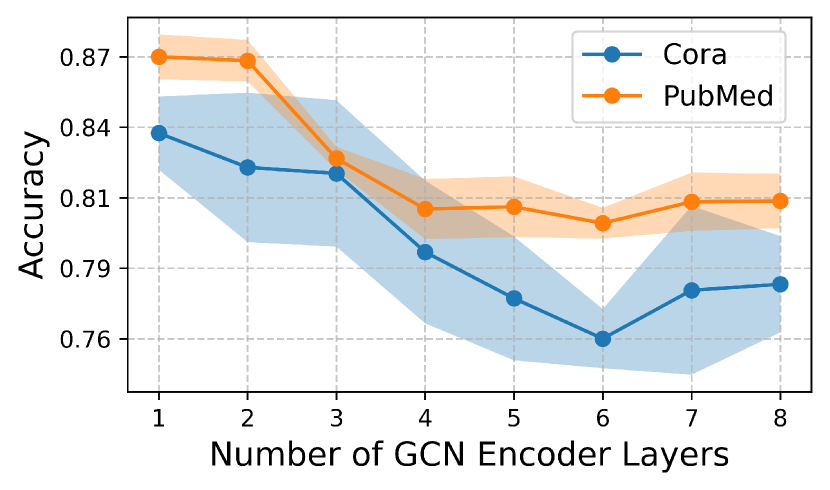
(a) G-BT on node CLS

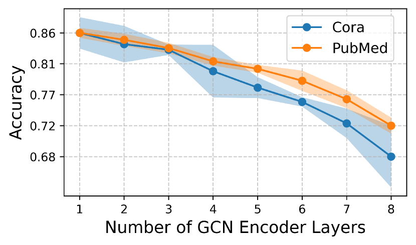
(b) MVGRL on node CLS

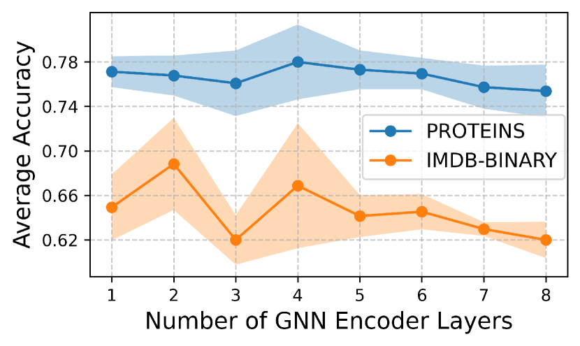
(c) G-BT on graph CLS

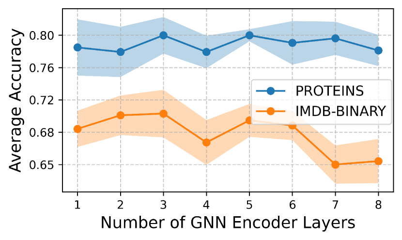
(d) MVGRL on graph CLS

Figure 1: Accuracy of CG-SSL v.s. number of GCN layers on node and graph classification on representative datasets. (a) G-BT on node classification. (b) MVGRL on node classification. (c) G-BT on graph classification. (d) MVGRL on graph classification. We choose two representative datasets for each task, i.e. Cora and CiteSeer for the node-level and PROTEINS and IMDB-BINARY for the graph-level classification. Definition of the accuracy of CG-SSL, details of datasets and other experimental settings are mentioned in Section 6.1.

By design, most GNN encoders primarily aggregate local neighborhood information through their layered structure, where each layer extends the receptive field by one hop. The depth of a GNN critically determines its ability to integrate information from various parts of the graph. With only a limited number of layers, a GNN’s receptive field is restricted to immediate neighborhoods (e.g., 1-hop or 2-hop distances). This limitation severely constrains the network’s ability to assimilate and leverage broader graph topologies or global features that are essential for encoding the spectral properties of the graph.

Limited implications for spectral augmentation in CG-SSL.

Given the limitations of shallow GNNs in capturing spectral information, the utility of spectral augmentation techniques in graph self-supervised learning settings warrants scrutiny. Spectral augmentation involves modifying the spectral components (e.g., eigenvalues and eigenvectors) of a graph to enrich the training process or to create diverse samples for enhancing learning robustness. However, if the primary encoder’s architecture—specifically, a shallow GNN—is intrinsically limited in its ability to perceive and process spectral properties, then the benefits of such augmentations are likely to be minimal.

5 Edge perturbation is all you need

So far, our findings indicate that spectral augmentation is not particularly effective in contrast-based graph self-supervised learning. It may suggest that spectral augmentation essentially amounts to random topology perturbation, based on significant contradictions in previous studies [16, 18, 36] and the theoretical insight that a shallow encoder can hardly capture spectral properties. In fact, most of the spectral augmentations are basically performing edge perturbations on the graph with some targeted directions. Since we preliminarily conclude that it is quite difficult for those augmentations to benefit from the spectral properties of graphs, it is very intuitive to hypothesize that edge perturbation itself matters in the learning process.

Consequently, we are turning back to Edge Perturbation (EP), a more straightforward and proven method for augmenting graph data. The two primary methods of edge perturbation are DropEdge and AddEdge. We want to claim that edge perturbation has a better performance than spectral augmentations and prove empirically that none of them actually or even can benefit much from any spectral information and properties. Also, we demonstrate edge perturbation is much more efficient in practical applications both for time and space sake, where spectral operations are almost infeasible. Overall, we will support the idea with evidence in the following sections that simple edge perturbation is not only good enough but even very optimal in contrast-based graph SSL and we don’t need to care about much for spectral cues.

Edge perturbation involves modifying the topology of the graph by either removing or adding edges at random. We detail the two main types of edge perturbation techniques used in our frameworks: edge dropping and edge adding.

DropEdge. Edge dropping is the process of randomly removing a subset of edges from the original graph to create an augmented view. Adopting the definition from [26], let $\mathcal{G}=(\mathbf{A},\mathbf{X})$ be the original graph with adjacency matrix $\mathbf{A}$. We introduce a mask matrix $\mathbf{M}$ of the same dimensions as $\mathbf{A}$, where each entry $M_{ij}$ follows a Bernoulli distribution with parameter $1-p$ (denoted as the drop rate). The edge-dropped graph $G^{\prime}$ is then obtained by element-wise multiplication of $\mathbf{A}$ with $\mathbf{M}$:

$$\mathbf{A}^{\prime}=\mathbf{A}\odot\mathbf{M}$$ (3)

where $\odot$ denotes the Hadamard product (element-wise multiplication).

AddEdge. Edge adding involves randomly adding a subset of new edges to the original graph to create an augmented view. Let $\mathbf{N}$ be an adding matrix of the same dimensions as $\mathbf{A}$, where each entry $N_{ij}$ follows a Bernoulli distribution with parameter $q$ (denoted as the add rate), and $N_{ij}=0$ for all existing edges in $\mathbf{A}$. The edge-added graph $\mathcal{G}^{\prime\prime}$ is obtained by adding $\mathbf{N}$ to $\mathbf{A}$:

$$\mathbf{A}^{\prime\prime}=\mathbf{A}+\mathbf{N}$$ (4)

These two operations ensure that the augmented views $\mathcal{G}^{(1)}$ and $\mathcal{G}^{(2)}$ have modified adjacency matrices $\mathbf{A}^{\prime}$ and $\mathbf{A}^{\prime\prime}$ respectively, which are used to generate contrastive views while preserving the feature matrix $\mathbf{X}$.

5.1 Advantage of edge perturbation over spectral augmentations

Edge perturbation offers several key advantages over spectral augmentation, making it a more effective and practical choice for contrast-based graph self-supervised learning. Compared to augmentations related to the graph spectrum, it has three major advantages.

Theoretically intuitive. Edge perturbation is inherently simpler and more intuitive. It directly modifies the graph’s structure by adding or removing edges, which aligns well with the shallow GNN encoders’ strength in capturing local neighborhood information. Given that shallow GNNs have a limited receptive field, they are better suited to leveraging the local structural changes introduced by edge perturbation rather than the global changes implied by spectral augmentation.

Significantly better efficiency. Edge perturbation methods such as edge dropping (DropEdge) and edge adding (AddEdge) are computationally efficient. Unlike spectral augmentation, which requires costly eigenvalue and eigenvector computations, edge perturbation can be implemented with basic graph operations. This efficiency translates to faster training and inference times, making it more suitable for large-scale graph datasets and real-time applications. As shown in Table 1, the time and space complexity of spectrum-related calculations are several orders of magnitude higher than those of simple edge perturbation operations. This makes spectrum-related calculations impractical for the large datasets typically encountered in real-world applications.

Table 1: Time and space complexity of different methods (Empirical Time is on PubMed dataset)

Method	Time Complexity	Space Complexity	Empirical Time (s/epoch)
Spectrum calculation	$O(n^{3})$	$O(n^{2})$	26.435
DropEdge	$O(m)$	$O(m)$	0.140
AddEdge	$O(m)$	$O(m)$	0.159

Optimal learning performance.

Most importantly and directly, our comprehensive empirical studies indicate that edge perturbation methods lead to significant improvements in model performance, as presented and analyzed in Sec. 6. From the results there, the conclusion can be drawn that the performance of the proposed augmentations is not only better than those of spectrum-related competitors but also matches or even surpasses the performance of other strong benchmarks.

These advantages position edge perturbation as a robust and efficient method for graph augmentation in self-supervised learning. In the following section, we will present our experimental analysis, demonstrating the accuracy gains achieved through edge perturbation methods.

6 Experiments on SSL performance

6.1 Experimental Settings.

Task and Datasets. We conducted extensive experiments for node-level classification on seven datasets: Cora, CiteSeer, PubMed [13], Photo, Computers [27], Coauthor-CS, and Coauthor-Phy. These datasets include various types of graphs, such as citation networks, co-purchase networks, and co-authored networks. Additionally, we carried out graph-level classification on five datasets from the TUDataset collection [21], which include biochemical molecules and social networks. More details of these datasets be found in Appendix B.

Baselines. We conducted experiments under four CG-SSL frameworks: MVGRL, GRACE, G-BT, and BGRL, using DropEdge, AddEdge, and SPAN [16] as augmentation strategies. For MVGRL, we also compared its original PPR augmentation. For the node classification task, we use GCA [43], GMI [24], DGI [30], and SpCo [18] as baselines. For the graph classification task, we use RGCL [15] and GraphCL [37] as baselines. The experimental details about the training configurations can be found in Appendix B

Evaluation Protocol. We adopt the evaluation and split scheme from previous works [31, 40, 16]. Each GNN encoder is trained on the entire graph with self-supervised learning. After training, we freeze the encoder and extract embeddings for all nodes or graphs. Finally, we train a simple linear classifier using the labels from the training/validation set and test it with the testing set. The accuracy of classification on the testing set shows how good the learned representations are. For the node classification task nodes are randomly divided into $10\%/10\%/80\%$ for training, validation, and testing, and for graph classification datasets, graphs are randomly divided into $80\%/10\%/10\%$ for training, validation, and testing.

6.2 Experimental results

We present the results of the node classification and graph classification tasks in Table 2 and Table 3, respectively. Our comparative analysis of graph augmentation for both node and graph classification reveals distinct performance trends. For node classification, DropEdge consistently achieves the best performance across multiple datasets and CG-SSL frameworks, demonstrating superior robustness and consistency. While AddEdge also achieves competitive accuracy, DropEdge stands out in this area. In graph classification, AddEdge frequently achieves the best performance across multiple datasets and CG-SSL frameworks, showing superior and more consistent results. In contrast, SPAN generally underperforms relative to both DropEdge and AddEdge  encountering scalability issues on larger datasets and suffering from a high overhead of training time.

Table 2: Node classification. Results of baselines with ’$\dagger$’ are adopted directly from previous works. MVGRL+PPR is the original setting of MVGRL. The best results in each cell are highlighted by grey. The best results overall are highlighted with bold and underline.

Model	Cora	CiteSeer	PubMed	Photo	Computers	Coauthor-CS	Coauthor-Phy
GCA†	83.67 $\pm$ 0.44	71.48 $\pm$ 0.26	78.87 $\pm$ 0.49	92.53 $\pm$ 0.16	88.94 $\pm$ 0.15	93.10 $\pm$ 0.01	—
GMI†	83.02 $\pm$ 0.33	72.45 $\pm$ 0.12	79.94 $\pm$ 0.25	90.68 $\pm$ 0.17	82.21 $\pm$ 0.31	91.08 $\pm$ 0.56	—
DGI†	82.34 $\pm$ 0.64	71.85 $\pm$ 0.74	76.82 $\pm$ 0.61	91.61 $\pm$ 0.22	83.95 $\pm$ 0.47	92.15 $\pm$ 0.63	—
SpCo†	84.30 $\pm$ 0.40	73.60 $\pm$ 1.10	81.50 $\pm$ 0.40	—	—	—	—
MVGRL + PPR	83.53 $\pm$ 1.19	71.56 $\pm$ 1.89	84.13 $\pm$ 0.26	88.47 $\pm$ 1.02	89.84 $\pm$ 0.12	90.57 $\pm$ 0.61	OOM
MVGRL + DropEdge	84.31 $\pm$ 1.95	74.85 $\pm$ 0.73	85.62 $\pm$ 0.45	89.28 $\pm$ 0.95	90.43 $\pm$ 0.33	93.20 $\pm$ 0.81	95.70 $\pm$ 0.28
MVGRL + AddEdge	83.21 $\pm$ 1.65	73.65 $\pm$ 1.60	84.86 $\pm$ 1.19	87.15 $\pm$ 1.36	87.59 $\pm$ 0.53	92.91 $\pm$ 0.65	95.33 $\pm$ 0.23
MVGRL +SPAN	84.57 $\pm$ 0.22	73.65 $\pm$ 1.29	85.21 $\pm$ 0.81	92.33 $\pm$ 0.99	88.75 $\pm$ 0.20	92.25 $\pm$ 0.76	OOM
G-BT + DropEdge	86.51 $\pm$ 2.04	72.95 $\pm$ 2.46	87.10 $\pm$ 1.21	93.55 $\pm$ 0.60	88.66 $\pm$ 0.46	93.31 $\pm$ 0.05	96.06 $\pm$ 0.24
G-BT + AddEdge	82.10 $\pm$ 1.48	66.36 $\pm$ 4.25	85.98 $\pm$ 0.81	93.68 $\pm$ 0.79	87.81 $\pm$ 0.79	91.98 $\pm$ 0.66	95.51 $\pm$ 0.02
G-BT + SPAN	84.06 $\pm$ 2.85	67.46 $\pm$ 3.18	85.97 $\pm$ 0.41	91.85 $\pm$ 0.22	88.73 $\pm$ 0.62	92.63 $\pm$ 0.07	OOM
GRACE + DropEdge	84.19 $\pm$ 2.07	75.44 $\pm$ 0.32	87.84 $\pm$ 0.37	92.62 $\pm$ 0.73	86.67 $\pm$ 0.61	93.15 $\pm$ 0.23	OOM
GRACE + AddEdge	85.78 $\pm$ 0.62	71.65 $\pm$ 1.63	85.25 $\pm$ 0.47	89.93 $\pm$ 0.74	76.74 $\pm$ 0.57	92.46 $\pm$ 0.25	OOM
GRACE + SPAN	82.84 $\pm$ 0.91	67.76 $\pm$ 0.21	85.11 $\pm$ 0.71	93.72 $\pm$ 0.21	88.71 $\pm$ 0.06	91.72 $\pm$ 1.75	OOM
BGRL + DropEdge	83.21 $\pm$ 3.29	71.46 $\pm$ 0.56	86.28 $\pm$ 0.13	92.90 $\pm$ 0.69	88.68 $\pm$ 0.65	91.58 $\pm$ 0.18	95.29 $\pm$ 0.19
BGRL + AddEdge	81.49 $\pm$ 1.21	69.66 $\pm$ 1.34	84.54 $\pm$ 0.22	91.85 $\pm$ 0.75	86.75 $\pm$ 1.15	91.78 $\pm$ 0.77	95.29 $\pm$ 0.09
BGRL + SPAN	83.33 $\pm$ 0.45	66.26 $\pm$ 0.92	85.97 $\pm$ 0.41	91.72 $\pm$ 1.75	88.61 $\pm$ 0.59	92.29 $\pm$ 0.59	OOM

Table 3: Graph classification. Results of baselines with ’$\dagger$’ are adopted directly from previous works. MVGRL+PPR is the original setting of MVGRL. The best results in each cell are highlighted by grey. The best results overall are highlighted with bold and underline.

Model	MUTAG	PROTEINS	NCI1	IMDB-BINARY	IMDB-MULTI
GraphCL†	86.80 $\pm$ 1.34	74.39 $\pm$ 0.45	77.87 $\pm$ 0.41	71.14 $\pm$ 0.44	48.58 $\pm$ 0.67
RGCL†	87.66 $\pm$ 1.01	75.03 $\pm$ 0.43	78.14 $\pm$ 1.08	71.85 $\pm$ 0.84	49.31 $\pm$ 0.42
MVGRL + PPR	90.00 $\pm$ 5.40	78.92 $\pm$ 1.83	78.78 $\pm$ 1.52	71.40 $\pm$ 4.17	52.13 $\pm$ 1.42
MVGRL+ SPAN	93.33 $\pm$ 2.22	79.81 $\pm$ 2.45	77.56 $\pm$ 1.77	75.00 $\pm$ 1.09	51.20 $\pm$ 1.62
MVGRL+ DropEdge	93.33 $\pm$ 2.22	78.92 $\pm$ 1.33	77.81 $\pm$ 1.50	76.40 $\pm$ 0.48	51.46 $\pm$ 3.02
MVGRL+ AddEdge	94.44 $\pm$ 3.51	81.25 $\pm$ 3.43	77.27 $\pm$ 0.71	74.00 $\pm$ 2.82	51.73 $\pm$ 2.43
G-BT + SPAN	90.00 $\pm$ 6.47	80.89 $\pm$ 3.22	78.29 $\pm$ 1.12	65.60 $\pm$ 1.35	45.60 $\pm$ 2.13
G-BT + DropEdge	92.59 $\pm$ 2.61	77.97 $\pm$ 0.42	78.18 $\pm$ 0.91	73.33 $\pm$ 1.24	49.11 $\pm$ 1.25
G-BT + AddEdge	92.59 $\pm$ 2.61	80.64 $\pm$ 1.68	75.91 $\pm$ 0.59	73.33 $\pm$ 1.24	48.88 $\pm$ 1.13
GRACE + SPAN	90.00 $\pm$ 4.15	79.10 $\pm$ 2.30	78.49 $\pm$ 0.79	70.80 $\pm$ 3.96	47.73 $\pm$ 1.71
GRACE + DropEdge	88.88 $\pm$ 3.51	78.21 $\pm$ 1.92	76.93 $\pm$ 1.14	71.00 $\pm$ 3.75	47.46 $\pm$ 3.02
GRACE + AddEdge	92.22 $\pm$ 4.44	80.17 $\pm$ 2.21	76.49 $\pm$ 1.25	69.96 $\pm$ 2.05	49.86 $\pm$ 4.09
BGRL + SPAN	90.00 $\pm$ 4.15	79.28 $\pm$ 2.73	78.05 $\pm$ 1.62	72.40 $\pm$ 2.57	47.46 $\pm$ 4.35
BGRL + DropEdge	88.88 $\pm$ 4.96	76.60 $\pm$ 2.21	76.15 $\pm$ 0.43	71.60 $\pm$ 3.31	51.47 $\pm$ 3.02
BGRL + AddEdge	91.11 $\pm$ 5.66	79.46 $\pm$ 2.18	76.98 $\pm$ 1.40	72.80 $\pm$ 2.48	47.77 $\pm$ 4.18

7 The insignificance of Spectral Cues

Given the superior empirical performance of edge perturbations mentioned in Sec. 6, one may still argue whether it is a result of some spectral cues or not, as all the analyses mentioned are not direct evidence of the insignificance of the spectral cues in the study. To clarify this, we have three questions to answer, (1) Can GNN encoders learn spectral information from augmented graphs produced edge perturbations? (2) Are spectrum in spectral augmentation necessary? (3) Is spectral information a significant factor in the performance of edge perturbation? Given the questions, we conduct a series of experimental studies to answer them respectively in Sec. 7.1, 7.2 and Appendix E.2.

7.1 Degeneration of the spectrum after EP

Here we want to conduct studies to answer the question of whether the GNN encoders applied can learn spectral information from the augmented graph views produced by EP. Therefore, we collect the spectrum of all augmented graphs ever produced along the way of the contrastive learning process of the best framework with the optimal parameter we have in this study, i.e. G-BT + EP with best drop rate $p$ or add rate $q$, and calculate the average one for each representative dataset in this study for both node- and graph-level tasks. We find that though the average spectrum of those original graphs is strikingly different, that of augmented graphs is quite similar for node- and graph-level tasks, respectively. This indicates a certain degree of degeneration of the spectra as they are no longer easy to separate after EP. Therefore, GNN encoders can hardly learn spectral information and properties between different original graphs from those augmented graph views. Note that, though we have defined some context of frameworks, this result is generally only dependent on the augmentation methods. Due to the limited space, we will elaborate and visualize the node-level results in this section and postpone the graph-level ones in Appendix E.1, as they support the claim very consistently.

Node-Level analysis.

Here, we visualize the distributions of the average spectrum of graphs at the node level using histograms. The spectral distribution for each graph is represented by a sorted vector of its eigenvalues. When referring to the average spectrum, we mean the average over the eigenvalue vectors of each augmented graph. We plot the histograms of different spectra, normalized to show the probability density. Note that eigenvalues are constrained within the range [0, 2], as we adopted the commonly used symmetrical normalization. We analyze the spectral distributions of three node classification datasets: Cora, CiteSeer, and Computers. We compare the average spectral properties of both original and augmented graphs. The augmentation method used is DropEdge, applied with optimal parameters identified for the G-BT method.

The results of the visualization are presented in Fig. 2. By comparing the spectrum distributions of original graphs for the datasets in Fig. 2(a), we can easily distinguish the spectra of the three datasets. This contrasts with the highly overlapped average spectra of all the datasets, indicating the degeneration mentioned. To support this claim, we also present the comparison of the spectra of original and augmented graphs on all three datasets in Fig. 2(c), 2(d), and 2(e), respectively, to show the obvious changes after the edge perturbations.

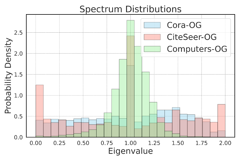
(a) Spectrum of original graphs

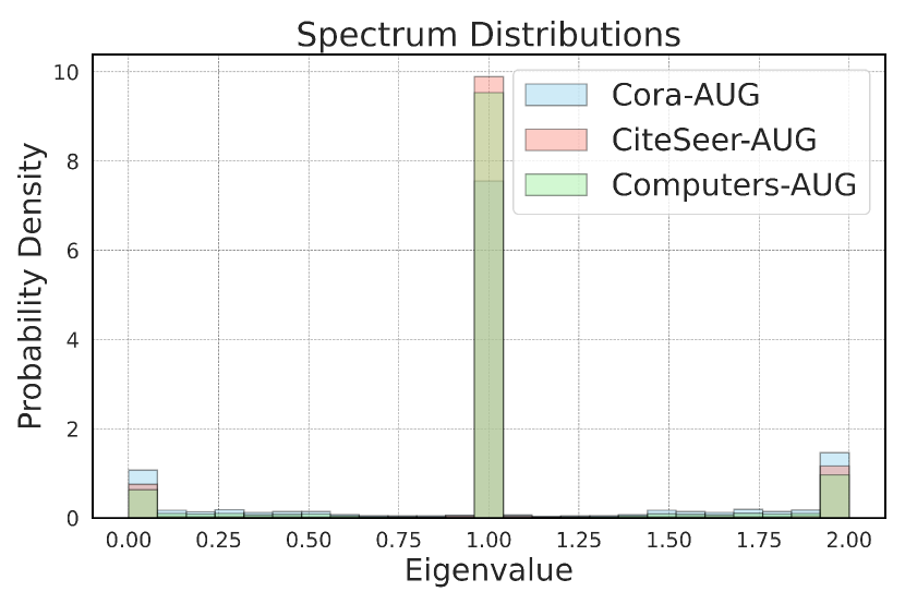
(b) Spectrum of augmented graphs

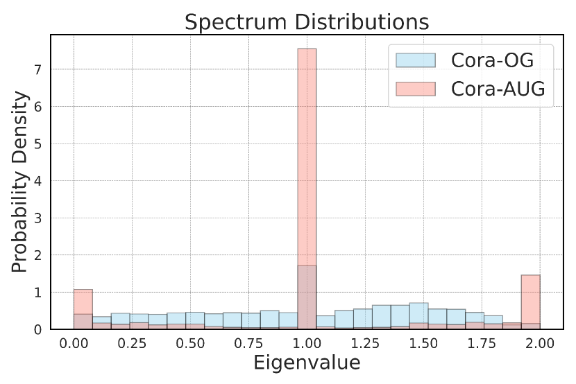
(c) Comparison on Cora

(d) Comparison on CiteSeer

(e) Comparison on Computers

Figure 2: The spectrum distributions of graphs on different node classification datasets. Cora, CiteSeer, and Computers are chosen as they are well representative of all the node classification datasets. OG means original graph and AUG means average augmented graphs. The augmentation method is DropEdge with the best parameter on G-BT method.

7.2 Spectral Perturbation

To further destruct the spectral properties from model performance, we introduce Spectral Perturbation Augmentor (SPA) for finer-grained anatomy. SPA performs random edge perturbation with an empirically negligible ratio $r_{SPA}$ to transform the input graph $\mathcal{G}$ into a new graph $\mathcal{G}_{SPA}$, such that $\mathcal{G}$ and $\mathcal{G}_{SPA}$ are close to each other topologically, while being divergent in the spectral space. The spectral divergence $d_{SPA}$ between $\mathcal{G}$ and $\mathcal{G}_{SPA}$ is measured by the $L_{2}$-distance of the respective spectra. With properly chosen hyperparameters $r_{SPA}$ and $d_{SPA}$, we view the augmented graph $\mathcal{G}_{SPA}$ as a doppelganger of $\mathcal{G}$ that preserves most of the graph-proximity, with only spectral information eliminated.

Spectral perturbation on spectral augmentation baselines.

SPAN, being a state-of-the-art spectral augmentation algorithm, demonstrated the correlation between graph spectra and model performance through designated perturbation on spectral priors. However, the effectiveness of simple edge perturbation motivated us to further investigate whether such a relationship is causational.

Specifically, for each pair of SPAN augmented graphs $\mathcal{G}^{1},\mathcal{G}^{2}$, we further augment them into $\mathcal{G}^{1}_{SPA},\mathcal{G}^{2}_{SPA}$ with our proposed SPA augmentor. The SPA-augmented training is performed under the same setup as SPAN, with graphs being SPA-augmented graphs $\mathcal{G}_{SPA}$. Experiment results in Fig 3 show that the effectiveness of graph augmentation can be preserved and, in some cases improved, even if the spectral information is destroyed.

SPAN, along with other spectral augmentation algorithms, can be formulated as an optimization on a parameterized $2$-step generative process:

$$s_{SPAN}\sim p_{\theta}\left(\boldsymbol{S}_{SPAN}\left.\right|\boldsymbol{\mathcal{G}}_{0}\right),\qquad\mathcal{G}_{SPAN}\sim p_{\phi}\left(\boldsymbol{\mathcal{G}}_{SPAN}\left.\right|\boldsymbol{S}_{SPAN}\right)$$ (5)

Given the property that $\mathcal{G}_{SPA}$ is topologically close to $\mathcal{G}_{SPAN}$ and the performance function $\text{P}=f\left(\mathcal{G}\right),\lim_{\mathcal{G}\rightarrow\mathcal{G}_{SPAN}}\text{P}\left(\mathcal{G}\right)=\text{P}\left(\mathcal{G}_{SPAN}\right)$, which indicates the continuity around $\mathcal{G}_{SPAN}$, we make a reasonable assertion that $\mathcal{G}_{SPA}$ comes from the same distribution as $\mathcal{G}_{SPAN}$. However, with their spectral space being enforced to be distant, $\mathcal{G}_{SPA}$ is almost impossible to be sampled from the same spectral augmentation generative process:

$$d_{SPA}\rightarrow\infty\implies p_{\theta}\left(s_{SPA}\left.\right|\boldsymbol{\mathcal{G}}_{0}\right)\rightarrow 0\implies p_{\theta,\phi}\left(\mathcal{G}_{SPA}\left.\right|\boldsymbol{\mathcal{G}}_{0}\right)\rightarrow 0$$ (6)

Although the constrained generative process in Eq. 5 does indicate some extent of causality between spectral distribution $\boldsymbol{S}$ and the spectral-augmented graph distribution $\boldsymbol{\mathcal{G}}_{SPAN}$, our experiment challenges a more essential and fundamental aspect of such reasoning: such causality exists upon pre-defined generative processes, which does not intrinsically exist in the graph distributions. Even worse, such constrained generative process is incapable of modeling the full distribution of $\boldsymbol{\mathcal{G}}_{SPAN}$ itself. In our experiment setup, all $\mathcal{G}_{SPA}$ serve as strong counter examples.

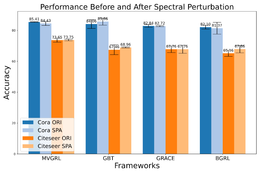
(a) Node classification

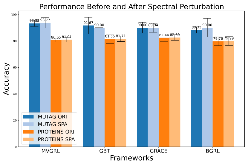
(b) Graph classification

Figure 3: Comparison of SPAN performance before and after applying SPA. After severely disrupting the spectral, the performance of SPAN is still comparable to that of the original version.

8 Conclusion

In this study, we investigate the effectiveness of spectral augmentation in contrast-based graph self-supervised learning (CG-SSL) frameworks to answer the question: Do spectral cues matter in CG-SSL? Our findings indicate that spectral information does not significantly enhance learning efficacy. Instead, simpler edge perturbation techniques, such as random edge dropping for node-level tasks and random edge adding for graph-level tasks, not only compete well but often outperform spectral augmentations. To be specific, we demonstrate that the benefits of spectral augmentation diminish with shallower networks, and edge perturbations yield superior performance in both node- and graph-level classification tasks. Additionally, GNN encoders struggle to learn spectral information from augmented graphs, and perturbing edges to alter spectral characteristics does not degrade model performance. These results challenge the current emphasis on spectral augmentation, advocating for more straightforward and effective edge perturbation techniques in CG-SSL, potentially reshaping the understanding and implementation of graph self-supervised learning.

Appendix A Limitations of the study

While our study provides compelling evidence against the necessity of spectral augmentation in contrast-based graph self-supervised learning (CG-SSL), it is important to acknowledge potential limitations that open avenues for further exploration.

1. Our analysis primarily focuses on specific types of edge perturbation techniques, i.e. DropEdge and AddEdge. Future research could explore a broader range of augmentation methods to validate our conclusions across different contexts.

2. Although we cover various state-of-the-art frameworks and tasks, the generalizability of our findings could be further strengthened by applying our approach to a wider range of datasets and frameworks.

3. Our conclusions are partially based on observations related to network depth. Though already adopted the most commonly used configuration among all related studies, further investigation is needed to understand how different network architectures and configurations might influence the effectiveness of spectral and edge-based augmentations.

Addressing these limitations can provide deeper insights and help refine graph self-supervised learning methodologies.

Appendix B Dataset and training configuration

Datasets. The node classification datasets used in this paper include the Cora, CiteSeer, and PubMed citation networks [13], as well as the Photo and Computers co-purchase networks [27]. Additionally, we use the Coauthor-CS and Coauthor-Phy co-author relationship networks. The statistics of node-level datasets are present in Table 4. The graph classification datasets include: The MUTAG dataset, which features seven types of graphs derived from 188 mutagenic compounds; the NCI1 dataset, which contains compounds tested for their ability to inhibit human tumor cell growth; the PROTEINS dataset, where nodes correspond to secondary structure elements connected if they are adjacent in 3D space; and the IMDB-BINARY and IMDB-MULTI movie collaboration datasets, where graphs depict interactions among actors and actresses, with edges denoting their collaborations in films. These movie graphs are labeled according to their genres. The statistics of graph-level datasets are present in Table 5. All datasets can be accessed through PyG library . All experiments are conducted using 8 NVIDIA A100 GPU.

Table 4: Statistics of node classification datasets

Dataset	#Nodes	#Edges	#Features	#Classes
Cora	2,708	5,429	1,433	7
CiteSeer	3,327	4,732	3,703	6
PubMed	19,717	44,338	500	3
Computers	13,752	245,861	767	10
Photo	7,650	119,081	745	8
Coauthor-CS	18,333	81,894	6,805	15
Coauthor-Phy	34,493	247,962	8,415	5

Table 5: Statistics of node classification datasets

Dataset	#Avg. Nodes	#Avg. Edges	# Graphs	#Classes
MUTAG	17.93	19.71	188	2
PROTEINS	39.06	72.82	1,113	2
NCI1	29.87	32.30	4110	2
IMDB-BINARY	19.8	96.53	1,000	2
IMDB-MULTI	13.0	65.94	1,500	5

Training configuration. For each CG-SSL framework, we implement it based on [41]  . We use the following hyperparameters: the learning rate is set to $5\times 10^{-4}$, and the node hidden size is set to $512$, the number of GCN encoder layer is set $\in\{1,2\}$. For all node classification datasets, training epochs are set $\in\{50,100,150,200,400,1000\}$, and for all graph classification datasets, training epochs are set $\in\{20,40,...,200\}$. To achieve performance closer to the global optimum, we use randomized search to determine the optimal probability of edge perturbation and SPAN perturbation ratio. For Cora and CiteSeer  the search is conducted one hundred times, and for all other datasets, it is conducted twenty times. For all graph classification datasets, the batch size is set to $128$.

Appendix C Preliminaries of Graph Spectrum and SPAN

Given a graph $\mathcal{G}=(\mathbf{A},\mathbf{X})$ with adjacency matrix $\mathbf{A}$ and feature matrix $\mathbf{X}$, we introduce some fundamental concepts related to the graph spectrum.

Laplacian Matrix Spectrum The Laplacian matrix $\mathbf{L}$ of a graph is defined as:

$$\mathbf{L}=\mathbf{D}-\mathbf{A}$$

where $\mathbf{D}$ is the degree matrix, a diagonal matrix where each diagonal element $D_{ii}$ represents the degree of vertex $i$. The eigenvalues of the Laplacian matrix, known as the Laplacian spectrum, are crucial in understanding the graph’s structural properties, such as its connectivity and the number of spanning trees [5].

Normalized Laplacian Spectrum The normalized Laplacian matrix $\mathbf{L}_{\text{norm}}$ is given by:

$$\mathbf{L}_{\text{norm}}=\mathbf{D}^{-1/2}\mathbf{L}\mathbf{D}^{-1/2}$$

The eigenvalues of the normalized Laplacian matrix, referred to as the normalized Laplacian spectrum, are often used in spectral clustering [32] and other applications where normalization is necessary to account for varying vertex degrees.

SPAN The core assumption of SPAN is to maximize the consistency of the representations of two views with a large spectrum distance, thereby filtering out edges sensitive to the spectrum, such as edges between clusters. By focusing on more stable structures relative to the spectrum, the objective of SPAN can be formulated as:

$$\max_{\boldsymbol{\mathcal{T}}_{1},\boldsymbol{\mathcal{T}}_{2}\in\mathcal{S}}\left\|\operatorname{eig}\left(\mathbf{L}_{1}\right)-\operatorname{eig}\left(\mathbf{L}_{2}\right)\right\|_{2}^{2}$$ (7)

where the transformations $\mathcal{T}_{1}$ and $\mathcal{T}_{2}$ convert $\mathbf{A}$ to $\mathbf{A}_{1}$ and $\mathbf{A}_{2}$, respectively, producing the normalized Laplacian matrices $\mathbf{L}_{1}$ and $\mathbf{L}_{2}$. Here, $\mathcal{S}$ represents the set of all possible transformations, and the graph spectrum can be calculated by $\operatorname{eig}\left(\mathbf{L}\right)$.

Appendix D Object function of GCL framework

Here we briefly introduce the object functions of the four CG-SSL frameworks used in this paper, for a more detailed discussion about object functions including other graph contrastive learning and graph self-supervised learning frameworks which can refer to the survey papers [34, 33, 19]. We use the following notations:

• $p_{\phi}$: Projection head parameterized by $\phi$.

• $\mathbf{h}_{i}$, $\mathbf{h}_{j}$: Representations of the graph nodes.

• $\mathbf{h}_{n}^{\prime}$: Representations of negative sample nodes.

• $\mathcal{P}$: Distribution of positive sample pairs.

• $\widetilde{\mathcal{P}}^{N}$: Distribution of negative sample pairs.

• $\mathcal{B}$: Set of nodes in a batch.

• $\mathbf{H}^{(\mathbf{1})}$, $\mathbf{H}^{(\mathbf{2})}$: Node representation matrices of two views.

GRACE uses the InfoNCE loss to maximize the similarity between positive pairs and minimize the similarity between negative pairs. InfoNCE loss encourages representations of positive pairs (generated from the same node via data augmentation) to be similar while pushing apart the representations of negative pairs (from different nodes). The loss function $\mathcal{L}_{\text{NCE }}$ denotes as:

$$\mathcal{L}_{\text{NCE }}\left(p_{\phi}\left(\mathbf{h}_{i},\mathbf{h}_{j}\right)\right)=-\mathbb{E}_{\mathcal{P}\times\widetilde{\mathcal{P}}^{N}}\left[\log\frac{e^{p_{\phi}\left(\mathbf{h}_{i},\mathbf{h}_{j}\right)}}{e^{p_{\phi}\left(\mathbf{h}_{i},\mathbf{h}_{j}\right)}+\sum_{n\in N}e^{p_{\phi}\left(\mathbf{h}_{i},\mathbf{h}_{n}^{\prime}\right)}}\right]$$ (8)

MVGRL employs the Jensen-Shannon Estimator (JSE) for contrastive learning, which focuses on the mutual information between positive pairs and negative pairs.JSE maximizes the mutual information between positive pairs and minimizes it for negative pairs, thus improving the representations’ alignment and uniformity. The loss function $\mathcal{L}_{\text{JSE }}$ denotes as:

$$\mathcal{L}_{\text{JSE }}\left(p_{\phi}\left(\mathbf{h}_{i},\mathbf{h}_{j}\right)\right)=\mathbb{E}_{\mathcal{P}\times\tilde{\mathcal{P}}}\left[\log\left(1-p_{\phi}\left(\mathbf{h}_{i},\mathbf{h}_{j}^{\prime}\right)\right)\right]-\mathbb{E}_{\mathcal{P}}\left[\log\left(p_{\phi}\left(\mathbf{h}_{i},\mathbf{h}_{j}\right)\right)\right]$$ (9)

BGRL utilizes a loss similar to BYOL, which does not require negative samples. It uses two networks, an online network and a target network, to predict one view from the other:

$$\mathcal{L}_{\text{BYOL }}\left(p_{\phi}\left(\mathbf{h}_{i},\mathbf{h}_{j}\right)\right)=\mathbb{E}_{\mathcal{P}\times\mathcal{P}}\left[2-2\cdot\frac{\left[p_{\phi}\left(\mathbf{h}_{i}\right)\right]^{T}\mathbf{h}_{j}}{\left\|p_{\phi}\left(\mathbf{h}_{i}\right)\right\|\left\|\mathbf{h}_{j}\right\|}\right]$$ (10)

G-BT applies the Barlow Twins’ loss to reduce redundancy in the learned representations, thereby ensuring better generalization:

$$\mathcal{L}_{\text{BT }}\left(\mathbf{H}^{(\mathbf{1})},\mathbf{H}^{(\mathbf{2})}\right)= \mathbb{E}_{\mathcal{B}\sim\mathcal{P}|\mathcal{B}|}\left[\sum_{a}\left(1-\frac{\sum_{i\in\mathcal{B}}\mathbf{H}_{ia}^{(1)}\mathbf{H}_{ia}^{(2)}}{\left\|\mathbf{H}_{ia}^{(1)}\right\|\left\|\mathbf{H}_{ia}^{(2)}\right\|}\right)^{2}\right.$$ (11)

$$\left.+\lambda\sum_{a}\sum_{b\neq a}\left(\frac{\sum_{i\in\mathcal{B}}\mathbf{H}_{ia}^{(1)}\mathbf{H}_{ib}^{(2)}}{\left\|\mathbf{H}_{ia}^{(1)}\right\|\left\|\mathbf{H}_{ib}^{(2)}\right\|}\right)^{2}\right].$$

Appendix E More experiments

E.1 Graph-Level analysis for degeneration of the spectrum after EP (Sec. 7.1 Cont.)

For graph-level analysis, we basically follow the settings mentioned above in node-level one. The only difference from the node-level task is that we have multiple original graphs with various numbers of nodes, leading to the inconsistent dimensions of the vector of the eigenvalues. Therefore, to provide a more detailed comparison of spectral properties at the graph level, we employ Kernel Density Estimation (KDE) [23] to interpolate and smooth the distributions of eigenvalues. We compare two groups of graph spectra. Each group’s spectra are processed to compute their KDEs, and the mean and standard deviation of these KDEs are calculated.

We analyze the spectral distributions of two node classification datasets: MUTAG and PROTEINS. We compare the average spectral properties of both original and augmented graphs. The augmentation method used is AddEdgeas it is the better among two EP methods, applied with optimal add rate identified for the G-BT method.

Like the results in node-level analysis, in Fig. 4(a) and 4(b), we witness the obvious difference between the average spectra of original graphs while the significant overlap between those of augmented graphs, especially if pay attention to the overlapping of the area created by the standard deviation of KDEs. Again, this contrast is not trivial because of the striking mismatch between the average spectra of original and augmented graphs in both datasets, as presented in Fig. 4(c) and 4(d).

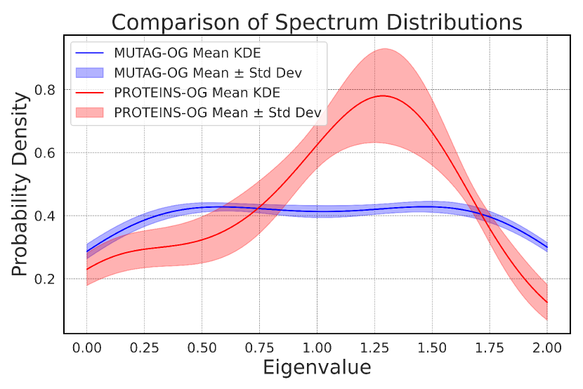
(a) Average spectra of original graphs

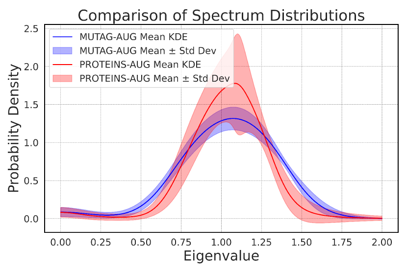
(b) Average spectra of augmented graphs

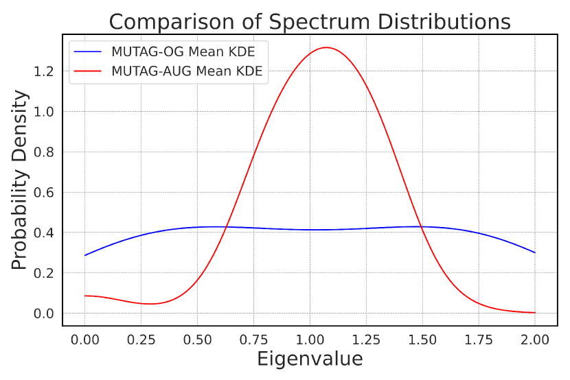
(c) The Spectrum of MUTAG

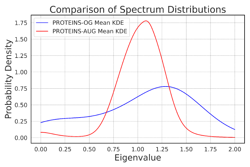
(d) The Spectrum of PROTEINS

Figure 4: The spectrum distributions of graphs on different graph classification datasets. MUTAG and PROTEINS are chosen as they are well representative of all the node classification datasets. OG means original graph and AUG means augmented graph. The augmentation method is AddEdge with the best parameter on G-BT method.

E.2 Relationship between spectral cues and performance of EP

Based on the findings obtained from Sec 7.1, it is very likely that spectral information can not be distinguishable enough for good representation learning on the graph. But to more directly answer the question of whether spectral cues play an important role in the learning performance of EP, we continue to conduct a statistical analysis to evaluate the influence of various factors on the learning performance. The results turn out to be consistent with our claim that spectral cues are insignificant aspects of outstanding performance on accuracy observed in Sec. 6.

E.2.1 Statistical analyses on key factors on performance of EP

From a statistical angle, we have a few dimensions of factors that can possibly influence learning performance, like the parameters of EP (i.e. drop rate $p$ in DropEdge or add rate $q$ in AddEdge) as well as potential spectral cues lying in the argument graphs. Therefore, to rule out the possibility that spectral cues are significant, comparisons are conducted on the impact of the parameters of EP in the augmentations versus:

1. The average $L_{2}$-distance between the spectrum of the original graph (OG) and that of each augmented graph (AUG) which is introduced by EP augmentations, denoted as OG-AUG.

2. The average $L_{2}$-distance between the spectra of a pair of augmented graphs appearing in the same learning epoch when having a two-way contrastive learning framework, like G-BT, denoted as AUG-AUG.

Two statistical analyses have been carried out to argue that the former is a more critical determinant and a more direct cause of the model efficacy. Each analysis was chosen for its ability to effectively dissect and compare the impact of edge perturbation parameters versus spectral changes.

Due to the high cost of calculating the spectrum of all AUGs in each epoch and the stability of the spectrum of the node-level dataset (as the original graph is fixed in the experiment), we perform this experiment on the contrastive framework and augmentation methods with the best performance in the study, i.e. G-BT with DropEdge on node-level classification. Also, we choose the small datasets, Cora  for analysis. Note that the smaller the graph, the higher the probability that the spectrum distance has a significant influence on the graph topology.

Analysis 1: Polynomial Regression.

Polynomial regression was utilized to directly model the relationship between the test accuracy of the model and the average spectral distances introduced by EP. This method captures the linear, or non-linear influences that these spectral distances may exert on the learning outcomes, thereby providing insight into how different parameters affect model performance.

Table 6: Polynomial regression of node-level accuracy over drop rate $p$ in DropEdge, average spectral distance between OG and AUG (OG-AUG), and average spectral distance between AUG pairs (AUG-AUG). The method is G-BT and the dataset is Cora. The best results are in grey.

Order of the regression	Regressor	R-squared $\uparrow$	Adj. R-squared $\uparrow$	F-statistic $\uparrow$	P-value $\downarrow$
1 (i.e. linear)	Drop rate $p$	0.628	0.621	81.12	6.94e-12
	OG-AUG	0.388	0.375	30.45	1.35e-06
	AUG-AUG	0.338	0.325	24.55	9.39e-06
2 (i.e. quadratic)	Drop rate $p$	0.844	0.837	126.9	1.14e-19
	OG-AUG	0.721	0.709	60.78	9.23e-14
	AUG-AUG	0.597	0.580	34.88	5.16e-10

The polynomial regression analysis in Table 6 highlights that the drop rate $q$ is the primary factor influencing model performance, showing strong and significant linear and non-linear relationships with test accuracy. In contrast, both the OG-AUG and AUG-AUG spectral distances have relatively minor impacts on performance, indicating that they are not significant determinants of the model’s efficacy.

Analysis 2: Instrumental Variable Regression.

To study the causal relationship, we perform an Instrumental Variable Regression (IVR) to rigorously evaluate the influence of spectral information and edge perturbation parameters on the performance of CG-SSL models. Specifically, we employ a Two-Stage Least Squares (IV2SLS) method to address potential endogeneity issues and obtain unbiased estimates of the causal effects.

In IV2SLS analysis, we define the variables as follows:

• Y (Dependent Variable): The outcome we aim to explain or predict, which in this case is the performance of the SSL model.

• X (Explanatory Variable): The variable that we believe directly influences Y. It is the primary factor whose effect on Y we want to measure.

• Z (Instrumental Variable): A variable that is correlated with X but not with the error term in the Y equation. It helps to isolate the variation in X that is exogenous, providing a means to obtain unbiased estimates of X’s effect on Y.

In this specific experiment, we conduct four separate regressions to compare the causal effects of these factors:

1. (X = AUG-AUG, Z = Parameter): Examines the relationship where the spectral distance between augmented graphs (AUG-AUG) is the explanatory variable (X) and edge perturbation parameters are the instrument (Z).

2. (X = Parameter, Z = AUG-AUG): Examines the relationship where the edge perturbation parameters are the explanatory variable (X) and the spectral distance between augmented graphs (AUG-AUG) is the instrument (Z).

3. (X = OG-AUG, Z = Parameter): Examines the relationship where the spectral distance between the original and augmented graphs (OG-AUG) is the explanatory variable (X) and edge perturbation parameters are the instrument (Z).

4. (X = Parameter, Z = OG-AUG): Examines the relationship where the edge perturbation parameters are the explanatory variable (X) and the spectral distance between the original and augmented graphs (OG-AUG) is the instrument (Z).

Table 7: IV2SLS regression results for the node-level task. The parameter $q$ refers to the drop rate in DropEdge. The experiment comes in pairs for each pair of variables and the better result is marked in grey.

Variable settings	R-squared $\uparrow$	F-statistic $\uparrow$	Prob (F-statistic) $\downarrow$
(X = AUG-AUG, Z = $q$)	0.341	45.77	1.68e-08
(Z = $q$ ,Z = AUG-AUG)	0.611	47.85	9.85e-09
(X = OG-AUG, Z = $q$)	0.250	40.22	7.51e-08
(X = $q$, Z = OG-AUG)	0.606	41.27	5.62e-08

The IV2SLS regression results for the node-level task in Table 7 indicate that the edge perturbation parameters are more significant determinants of model performance than spectral distances. Specifically, when the spectral distance between augmented graphs (AUG-AUG) is the explanatory variable (X) and drop rate $q$ are the instrument (Z), the model explains 34.1% of the variance in performance (R-squared = 0.341). Conversely, when the roles are reversed (X = $q$, Z = AUG-AUG), the model explains 61.1% of the variance (R-squared = 0.611), indicating a stronger influence of edge perturbation parameter $q$. A similar conclusion can be made when comparing OG-AUG and $q$.

Summary of Regression Analyses

The analyses distinctly show that the direct edge perturbation parameters have a consistently stronger and more significant impact on model performance than the two types of spectral distances that serve as a reflection of spectral cues. The results support the argument that while spectral cues might have contributed to model performance, its significance is extremely limited and the parameters of the EP methods themselves are more critical determinants.

References

- [1] Mohamed Ishmael Belghazi, Aristide Baratin, Sai Rajeshwar, Sherjil Ozair, Yoshua Bengio, Aaron Courville, and Devon Hjelm. Mutual information neural estimation. In International conference on machine learning, pages 531–540. PMLR, 2018.
- [2] Deyu Bo, Yuan Fang, Yang Liu, and Chuan Shi. Graph contrastive learning with stable and scalable spectral encoding. In Thirty-seventh Conference on Neural Information Processing Systems, 2023.
- [3] Ting Chen, Simon Kornblith, Mohammad Norouzi, and Geoffrey Hinton. A simple framework for contrastive learning of visual representations. In International conference on machine learning, pages 1597–1607. PMLR, 2020.
- [4] Zhengdao Chen, Lei Chen, Soledad Villar, and Joan Bruna. Can graph neural networks count substructures? Advances in neural information processing systems, 33:10383–10395, 2020.
- [5] Fan RK Chung. Spectral graph theory, volume 92. American Mathematical Soc., 1997.
- [6] Jacob Devlin, Ming-Wei Chang, Kenton Lee, and Kristina Toutanova. Bert: Pre-training of deep bidirectional transformers for language understanding. arXiv preprint arXiv:1810.04805, 2018.
- [7] Jean-Bastien Grill, Florian Strub, Florent Altché, Corentin Tallec, Pierre Richemond, Elena Buchatskaya, Carl Doersch, Bernardo Avila Pires, Zhaohan Guo, Mohammad Gheshlaghi Azar, et al. Bootstrap your own latent-a new approach to self-supervised learning. Advances in neural information processing systems, 33:21271–21284, 2020.
- [8] Xiaojun Guo, Yifei Wang, Zeming Wei, and Yisen Wang. Architecture matters: Uncovering implicit mechanisms in graph contrastive learning. Advances in Neural Information Processing Systems, 36, 2024.
- [9] Michael Gutmann and Aapo Hyvärinen. Noise-contrastive estimation: A new estimation principle for unnormalized statistical models. In Proceedings of the thirteenth international conference on artificial intelligence and statistics, pages 297–304. JMLR Workshop and Conference Proceedings, 2010.
- [10] Will Hamilton, Zhitao Ying, and Jure Leskovec. Inductive representation learning on large graphs. Advances in neural information processing systems, 30, 2017.
- [11] Kaveh Hassani and Amir Hosein Khasahmadi. Contrastive multi-view representation learning on graphs. In International conference on machine learning, pages 4116–4126. PMLR, 2020.
- [12] Wengong Jin, Regina Barzilay, and Tommi Jaakkola. Junction tree variational autoencoder for molecular graph generation. In International conference on machine learning, pages 2323–2332. PMLR, 2018.
- [13] Thomas N Kipf and Max Welling. Semi-supervised classification with graph convolutional networks. arXiv preprint arXiv:1609.02907, 2016.
- [14] Taewook Ko, Yoonhyuk Choi, and Chong-Kwon Kim. Universal graph contrastive learning with a novel laplacian perturbation. In Uncertainty in Artificial Intelligence, pages 1098–1108. PMLR, 2023.
- [15] Sihang Li, Xiang Wang, An Zhang, Yingxin Wu, Xiangnan He, and Tat-Seng Chua. Let invariant rationale discovery inspire graph contrastive learning. In International conference on machine learning, pages 13052–13065. PMLR, 2022.
- [16] Lu Lin, Jinghui Chen, and Hongning Wang. Spectral augmentation for self-supervised learning on graphs. In The Eleventh International Conference on Learning Representations, 2023.
- [17] Minhua Lin, Teng Xiao, Enyan Dai, Xiang Zhang, and Suhang Wang. Certifiably robust graph contrastive learning. Advances in Neural Information Processing Systems, 36, 2024.
- [18] Nian Liu, Xiao Wang, Deyu Bo, Chuan Shi, and Jian Pei. Revisiting graph contrastive learning from the perspective of graph spectrum. In Alice H. Oh, Alekh Agarwal, Danielle Belgrave, and Kyunghyun Cho, editors, Advances in Neural Information Processing Systems, 2022.
- [19] Yixin Liu, Ming Jin, Shirui Pan, Chuan Zhou, Yu Zheng, Feng Xia, and S Yu Philip. Graph self-supervised learning: A survey. IEEE transactions on knowledge and data engineering, 35(6):5879–5900, 2022.
- [20] Yixin Liu, Ming Jin, Shirui Pan, Chuan Zhou, Yu Zheng, Feng Xia, and Philip S. Yu. Graph self-supervised learning: A survey. IEEE Transactions on Knowledge and Data Engineering, 35(6):5879–5900, 2023.
- [21] Christopher Morris, Nils M Kriege, Franka Bause, Kristian Kersting, Petra Mutzel, and Marion Neumann. Tudataset: A collection of benchmark datasets for learning with graphs. arXiv preprint arXiv:2007.08663, 2020.
- [22] Sebastian Nowozin, Botond Cseke, and Ryota Tomioka. f-gan: Training generative neural samplers using variational divergence minimization. Advances in neural information processing systems, 29, 2016.
- [23] Emanuel Parzen. On estimation of a probability density function and mode. The annals of mathematical statistics, 33(3):1065–1076, 1962.
- [24] Zhen Peng, Wenbing Huang, Minnan Luo, Qinghua Zheng, Yu Rong, Tingyang Xu, and Junzhou Huang. Graph representation learning via graphical mutual information maximization. In Proceedings of The Web Conference 2020, pages 259–270, 2020.
- [25] Jiezhong Qiu, Qibin Chen, Yuxiao Dong, Jing Zhang, Hongxia Yang, Ming Ding, Kuansan Wang, and Jie Tang. Gcc: Graph contrastive coding for graph neural network pre-training. In Proceedings of the 26th ACM SIGKDD international conference on knowledge discovery & data mining, pages 1150–1160, 2020.
- [26] Yu Rong, Wenbing Huang, Tingyang Xu, and Junzhou Huang. Dropedge: Towards deep graph convolutional networks on node classification. In International Conference on Learning Representations, 2020.
- [27] Oleksandr Shchur, Maximilian Mumme, Aleksandar Bojchevski, and Stephan Günnemann. Pitfalls of graph neural network evaluation. arXiv preprint arXiv:1811.05868, 2018.
- [28] Fan-Yun Sun, Jordan Hoffmann, Vikas Verma, and Jian Tang. Infograph: Unsupervised and semi-supervised graph-level representation learning via mutual information maximization. arXiv preprint arXiv:1908.01000, 2019.
- [29] Shantanu Thakoor, Corentin Tallec, Mohammad Gheshlaghi Azar, Rémi Munos, Petar Veličković, and Michal Valko. Bootstrapped representation learning on graphs. In ICLR 2021 Workshop on Geometrical and Topological Representation Learning, 2021.
- [30] Petar Velickovic, William Fedus, William L Hamilton, Pietro Liò, Yoshua Bengio, and R Devon Hjelm. Deep graph infomax. ICLR (Poster), 2(3):4, 2019.
- [31] Petar Veličković, William Fedus, William L. Hamilton, Pietro Liò, Yoshua Bengio, and R Devon Hjelm. Deep graph infomax. In International Conference on Learning Representations, 2019.
- [32] Ulrike Von Luxburg. A tutorial on spectral clustering. Statistics and computing, 17:395–416, 2007.
- [33] Lirong Wu, Haitao Lin, Cheng Tan, Zhangyang Gao, and Stan Z Li. Self-supervised learning on graphs: Contrastive, generative, or predictive. IEEE Transactions on Knowledge and Data Engineering, 35(4):4216–4235, 2021.
- [34] Yaochen Xie, Zhao Xu, Jingtun Zhang, Zhengyang Wang, and Shuiwang Ji. Self-supervised learning of graph neural networks: A unified review. IEEE transactions on pattern analysis and machine intelligence, 45(2):2412–2429, 2022.
- [35] Danfei Xu, Yuke Zhu, Christopher B Choy, and Li Fei-Fei. Scene graph generation by iterative message passing. In Proceedings of the IEEE conference on computer vision and pattern recognition, pages 5410–5419, 2017.
- [36] Kaiqi Yang, Haoyu Han, Wei Jin, and Hui Liu. Augment with care: Enhancing graph contrastive learning with selective spectrum perturbation, 2023.
- [37] Yuning You, Tianlong Chen, Yongduo Sui, Ting Chen, Zhangyang Wang, and Yang Shen. Graph contrastive learning with augmentations. Advances in neural information processing systems, 33:5812–5823, 2020.
- [38] Yue Yu, Xiao Wang, Mengmei Zhang, Nian Liu, and Chuan Shi. Provable training for graph contrastive learning. Advances in Neural Information Processing Systems, 36, 2024.
- [39] Jure Zbontar, Li Jing, Ishan Misra, Yann LeCun, and Stéphane Deny. Barlow twins: Self-supervised learning via redundancy reduction. In International conference on machine learning, pages 12310–12320. PMLR, 2021.
- [40] Yifei Zhang, Hao Zhu, Zixing Song, Piotr Koniusz, and Irwin King. Spectral feature augmentation for graph contrastive learning and beyond. In Proceedings of the AAAI Conference on Artificial Intelligence, volume 37, pages 11289–11297, 2023.
- [41] Yanqiao Zhu, Yichen Xu, Qiang Liu, and Shu Wu. An empirical study of graph contrastive learning. NeurIPS, 2021.
- [42] Yanqiao Zhu, Yichen Xu, Feng Yu, Qiang Liu, Shu Wu, and Liang Wang. Deep graph contrastive representation learning. arXiv preprint arXiv:2006.04131, 2020.
- [43] Yanqiao Zhu, Yichen Xu, Feng Yu, Qiang Liu, Shu Wu, and Liang Wang. Graph contrastive learning with adaptive augmentation. In Proceedings of the Web Conference 2021, pages 2069–2080, 2021.