Hybrid Quantum Algorithm for Simulating Real-Time Thermal Correlation Functions
Abstract
We present a hybrid Path Integral Monte Carlo (hPIMC) algorithm to calculate real-time quantum thermal correlation functions and demonstrate its application to open quantum systems. The hPIMC algorithm leverages the successes of classical PIMC as a computational tool for high-dimensional system studies by exactly simulating dissipation using the Feynman-Vernon influence functional on a classical computer. We achieve a quantum speed-up over the classical algorithm by computing short-time matrix elements of the quantum propagator on a quantum computer. We show that the component of imaginary-time evolution can be performed accurately using the recently developed Probabilistic Imaginary-Time Evolution (PITE) algorithm, and we introduce a novel low-depth circuit for approximate real-time evolution under the kinetic energy operator using a Discrete Variable Representation (DVR). We test the accuracy of the approximation by computing the position-position thermal correlation function of a proton transfer reaction.
I Introduction
Noisy intermediate-scale quantum (NISQ) computers are characterized by small qubit counts and short coherence times [1]. Algorithms designed for NISQ era hardware must therefore operate within the constraints of limited qubits and low-depth circuits. One way this achieved is by using so-called hybrid quantum algorithms in which inexpensive subroutines are performed classically while expensive, quantum-in-nature calculations are off-loaded to a quantum computer. The most thoroughly explored approaches to hybrid algorithm design are variational quantum algorithms (VQAs), which are inspired by classical variational optimization [2, 3, 4, 5, 6, 7, 8, 9, 10, 11]. Although VQAs succeed in achieving shallow quantum circuits, they often scale poorly with system size due to the emergence of barren plateaus and their performance is limited by the expressiveness of their variational ansatz [12, 13, 14].
Recently, Layden et al. proposed a hybrid algorithm based on Markov chain Monte Carlo and Metropolis-Hasting acceptance/rejection criteria, and demonstrated that it achieves a quantum speedup over classical methods for sampling the Boltzmann distribution of an Ising spin model [15]. A related method, used to compute dynamical quantities, is Path Integral Monte Carlo (PIMC). In this paper, we propose the first hybrid PIMC (hPIMC) algorithm and show that it achieves a quantum speedup in the calculation of real-time thermal correlation functions (TCFs) for open quantum systems. Importantly, like Layden’s algorithm, hPIMC does not rely on variational techniques and therefore offers a new avenue for exploring chemical dynamics with hybrid computing.
Open quantum systems typically comprise a quantum mechanical system that interacts with and dissipates energy to an external environment that can, in turn, drive the system dynamics. Classical PIMC methods often involve computing short-time matrix elements of the system time-evolution operator (real-time in the case of zero temperature and complex-time for finite temperature simulations) by diagonalizing the Hamiltonian in a first-quantized representation for an arbitrary potential energy surface, and then incorporating the effects of the environment exactly through the Feynman-Vernon influence functional [16, 17, 18, 19, 20, 21]. Although classical PIMC approaches have been used for relatively high dimensional simulations, typically this represents a significant increase in the number of environment degrees of freedom while the system remains low-dimensional, with only a couple continuous degrees of freedom representing the limit beyond which calculation of the system time-evolution operator (TEO) matrix elements become unfeasible.
The central ideas of the hPIMC approach are to (i) use a quantum computer to push the boundaries of the system size limitations and (ii) leverage the fact that in the path integral framework, [21] only short-time TEO matrix elements are required, eliminating cumulative errors on the quantum computer due to successive applications of short-time quantum propagation steps. We use these ideas to construct a hybrid Monte Carlo algorithm where operations such as sampling random paths and evaluating acceptance/rejection criteria are carried out classically, while the expensive task of computing TEO matrix elements is achieved using a low-depth quantum circuit.
In what follows, we introduce hPIMC for equilibrium systems in an arbitrary representation and show that it achieves a quantum speedup compared with classical PIMC for computing real-time TCFs. We then adapt the hPIMC algorithm to condensed phase systems modeled by the Caldeira-Leggett (CL) Hamiltonian in position space and introduce an influence functional to capture dissipative effects. We also discuss the use of the PITE algorithm [22, 23] for imaginary-time evolution of the TEO matrix elements necessary for systems at finite temperature initially in thermal equilibrium. We further propose a new approach to approximate system propagation under the kinetic energy operator using a discrete variable representation (DVR) [24, 25, 26] and prove an algorithm for doing so. We test the accuracy of this approximation with classical simulations of the position TCF of a proton transfer reaction.
II Theory
We start with a symmetrized real-time TCF between two operators, and , at time for a system at equilibrium,
| (1) |
where is the complex-time evolution operator, is the system Hamiltonian, and where , is the Boltzmann constant, and is temperature. Throughout, we work in atomic units so that . In a PIMC calculation, the partition function, , can be computed through a separate normalization calculation [20, 19], and we do not explicitly address methods of computing it here.
In most cases, finding an exact representation of is not possible, and approximations are used instead. Let be an approximation to such that the error is bound by
| (2) |
where is the matrix 1-norm or trace norm. Further, let be an approximation to in which is used in place of . We show in Supplemental Material, Sec. I that the error, , made from approximating is on the order,
| (3) |
Within the path integral framework is discretized into a product of short-time system TEOs
| (4) |
where is the number of Trotter steps, and . In order to evaluate , we insert copies of identity using a complete basis, , into Eq. (4); the choice of basis here is arbitrary. The resulting expression for the TCF is,
| (5) |
where is a set of indices and at each Trotter step, indexed by , we sum over the entire basis set. Note that due to the trace. We sample path space in by defining the product
| (6) |
and normalization factor
| (7) |
where . This allows us to express Eq. (II) in the conventional PIMC form of an expectation value over a distribution, , which we use for importance sampling:
| (8) |
where . We note that can be computed concurrently with .
Evaluating with Monte Carlo introduces an additional source of error, , which is dependent on the Monte Carlo sampling rate of convergence. In general, for Monte Carlo iterations, this error is given by
| (9) |
We note that although Eq. (9) holds in the asymptotic limit, the true rate of convergence is more complicated and not easy to express since for small systems with no significant dissipation, the well-established sign problem in quantum dynamics must be considered [27].
In order to tie together both sources of error, we let the total error of computing Eq. (1) be divided equally between contributions from and so that
| (10) |
where is the total error. To ensure accuracy from Monte Carlo, we require at least Monte Carlo iterations. We would also like to find a way to relate to the number of Trotter steps, however, this will depend on the choice of approximation used to implement . For example, when the Hamiltonian has the form with non-commuting and , can be approximated with a th-order Suzuki product [28]. In this case, to ensure accuracy from approximating as , the number of Trotter steps must be at least
| (11) |
where
| (12) |
We now estimate the runtime and space complexity of computing using classical PIMC and hPIMC. In either case, within each Monte Carlo iteration, two random strings of matrix elements, and , referred to as the forward and backward paths, respectively, are sampled and the TCF estimators are computed. For classical PIMC, the TEO matrix elements are found by diagonalizing the Hamiltonian expressed in a chosen finite basis. For a -dimensional system and using a basis set of size , the one-time cost of diagonalization is and space in memory is required to store the result. We assume that the cost to compute and store and is at most on the same order of . For every Monte Carlo iteration, elementary operations are needed to compute Eq. (4) for given forward and backward paths. The total cost for classical PIMC is therefore
| (13) | |||
For hPIMC we propose to compute each TEO matrix element individually on the quantum computer, thus avoiding the need to diagonalize . We therefore trade the exponential cost of diagonalization for calls to a quantum oracle that implements . The efficiency of hPIMC therefore depends on the efficiency of the oracle. However, for many important chemical systems, efficient implementations of in terms of both runtime and space complexity are known [29, 30, 31, 32, 9, 33, 34, 4]. We assume that and can be computed classically with negligible cost. To represent each on a quantum computer, quantum registers, each consisting of qubits, are needed. The total cost of hPIMC is therefore
| (14) | ||||
where and are the cost and number of ancillary qubits, respectively, needed to call an oracle that implements . From this analysis, we see that hPIMC scales exponentially better in terms of both space and runtime complexity compared to classical PIMC. Additionally, because each TEO matrix element involves only a single application of , the quantum circuit is low depth and cumulative error from computing a series of on a noisy quantum computer is avoided.
We note that we can further improve the performance of hPIMC by storing TEO matrix elements in a classical look-up table and querying it each Monte Carlo iteration. Then, the distribution between classical and quantum resources becomes increasingly more classical as the calculation progresses and the table fills up. Further, employing problem-specific sampling techniques will likely allow us to target the most relevant Hilbert subspace, keeping the table from becoming exponentially large.
Finally, it is clear that hPIMC offers a significant advantage over VQAs in that for a fixed number of qubits, the error can be systematically reduced without increasing the depth of the quantum circuit by running more Monte Carlo iterations, as shown in Eq. (9), or increasing . This is not the case for VQAs: for a fixed number of qubits, and assuming that the classical optimizer has found the best solution, the error of a VQA is related to the expressiveness of the variational ansatz. Increasing the expressiveness, and thereby reducing the error, requires adding more gates to the variational ansatz, which increases circuit depth.
III Open Quantum Systems
Much of the success of classical PIMC has been in the context of dissipative systems at finite temperature where the rapid damping of quantum system oscillations by coupling to a large number of environment degrees of freedom significantly reduces the dynamical sign problem. This motivates us to adapt hPIMC for condensed phase dynamics described by the CL Hamiltonian using a position space representation. Specifically, the CL Hamiltonian describes a primary system consisting of modes in physical dimensions bilinearly coupled to an isotropic bath approximated by harmonic modes,
| (15) |
where is the system sub-Hamiltonian shifted along the adiabatic path and is the bath sub-Hamiltonian modified to include the system-bath coupling term [18]. It has been shown that for this choice of sub-Hamiltonians the error made by approximating the TEO as
| (16) |
goes as , where depends on the adiabaticity of the bath and goes to zero in the limit that the bath responds instantaneously to the system [16].
Another reason for expressing the CL Hamiltonian in this way is that in a position space representation, all terms involving contributions from the bath can be collected and integrated analytically, yielding the Feynman-Vernon influence functional [35]. Assuming and are functions only of position, the TCF of Eq. (15) becomes
| (17) |
where is the influence functional and we define the forward path, , the backward path, , and . We also define the product of forward and backward path matrix elements
| (18) |
and
| (19) |
respectively. Monte Carlo importance sampling is performed using and in Eqs. (6-8). Before integrating out the bath degrees of freedom, the integral in Eq. (17) is dimensional. To accurately model the bath using Eq. (15) we typically have . Using the influence functional reduces the dimensionality of the integral to , which is the dimensionality of the same system if it were in the gas phase. The influence functional can be computed on a classical computer with negligible cost.
We can approximate the continuous integrals in Eq. (17) as discrete sums over a finite width grids of evenly spaced grid points. In one dimension, let be the total length of the grid and the number of grid points. Any position on the grid is given by , where , , and is the set of integers . We represent the grid on a quantum computer by mapping to the computational basis:
| (20) |
where are the binary expansion coefficients of and . Here, represents a single quantum register. For dimensions, each position coordinate is mapped to its own quantum register and the overall state is the direct product of all registers. The constant offset, , and grid spacing, , are absorbed into the implementation of the potential energy [36]. Because we are mapping positions on a grid directly to the computational basis, each register can be efficiently initialized with a single layer of Pauli-X gates.
We compute the real and imaginary parts of , where now , on a quantum computer using a standard Hadamard test [37]. In doing so, we split the TEO into a product of real and imaginary-time TEOs,
| (21) |
where and . We perform imaginary-time evolution using the PITE algorithm [22, 23]. For an initial state and a single ancilla qubit, PITE takes as input a circuit that executes real-time evolution, , and approximates evolution in imaginary-time by the unitary such that
| (22) |
where , , and is a real parameter. When the ancillary qubit is measured in the state , is evolved in imaginary-time by a first-order approximation to . Note that the probability of successfully measuring increases for smaller values of . PITE was originally designed for finding the ground state of an input Hamiltonian where successive applications of the circuit are needed to reach larger , each of which lowers the probability of success. However, in hPIMC, is inherently small to ensure that Eq. (16) is a good approximation. Thus we only require a single application of PITE per TEO matrix element which means the additional overhead from calling PITE until a successful outcome is measured is minimal.
For evolution in real-time, we approximate the TEO using a second-order Trotter splitting, [38]
| (23) |
In the position basis, is diagonal and can be constructed efficiently if there exists a classical algorithm that efficiently implements [39]. For example, quadratic potentials with linear coupling can be constructed with one- and two-qubit gates. [36]
Although the CL Hamiltonian described here includes only a single electronic state potential energy surface, we note that hPIMC can easily be extended to nonadiabatic systems that employ a diabatic representation for multiple potential energy surfaces following the work in [4]. We expect hPIMC to provide a useful tool for studies of condensed phase nonadiabatic systems in which the electronic state transitions are strongly coupled to multiple vibrational degrees of freedom, but save this investigation for future work.
IV DVR Approximation
We propose to evaluate time evolution under the kinetic energy operator with a discrete variable representation (DVR) of . The DVR of the kinetic energy operator expressed using a sinc basis set is given by [24]
| (24) |
where
| (25) |
Here, is a tensor product of identity matrices and the DVR of the th system mode in one dimension is defined by the matrix elements
| (26) |
where is the mass of the th system mode. In the limit where goes to zero, this approximation is exact.
Ordinarily, one diagonalizes the DVR Hamiltonian, , and performs dynamics in the basis of DVR eigenvectors. However, in hPIMC, we avoid diagonalizing by approximating evolution under as . That is,
| (27) |
Since DVR is not typically used this way, we present results in the next section that validate this approach.
In general, we cannot efficiently implement on a quantum computer because is dense. At the same time, we can see from Eq. (26) that the matrix elements decrease in magnitude moving away from the main diagonal, and should eventually become small enough to safely neglect. In Supplemental Material, Sec. II, we prove that this is indeed the case and find that for a given error tolerance, , can be made sparse by neglecting all diagonals, , where , and is given by
| (28) |
with . Here, is the main diagonal, are the adjacent upper and lower diagonals, and so on. Formally, this expression results from a lower bound on error; however, we show in Supplemental Material, Sec. II that this bound is tight.
We can then simulate time evolution under using a first-order Trotter splitting about the diagonals of :
| (29) |
where gives the input matrix with all elements neglected except those on the th diagonals. Each matrix is 2-sparse and in Supplemental Material, Sec. III we prove that each of these 2-sparse matrices can be decomposed into a sum of at most two 1-sparse matrices. Our method yields a factor of 12 improvement compared to the results of [28] for a 2-sparse matrix. Using a first-order Trotter splitting about each 1-sparse matrix yields
| (30) |
where indexes the 1-sparse matrices resulting from the decomposition. From here, each 1-sparse matrix can be directly simulated with just two black-box queries to [39, 40]. In total, Eq. (27) can be simulated with at most black-box queries.
V Results and Conclusion
Our proposed method to simulate the system TEO involves several approximations, and although the error from some of these approximations can be analyzed individually, rigorously studying the cumulative error is not straightforward. Instead, we investigate the resulting error by computing the position-position TCF of a proton transfer reaction using the approach outlined above and compare the results to the exact ones obtained by diagonalization. We model the donor and acceptor sites of the reaction using a standard symmetric double-well potential:
| (31) |
Real-time evolution is approximated with a second-order Trotter splitting, as in Eq. (23), and imaginary-time evolution is approximated with a first-order Trotter splitting to replicate PITE. We evaluate the TCF using quadrature to avoid Monte Carlo error. All results are obtained with a classical computer.
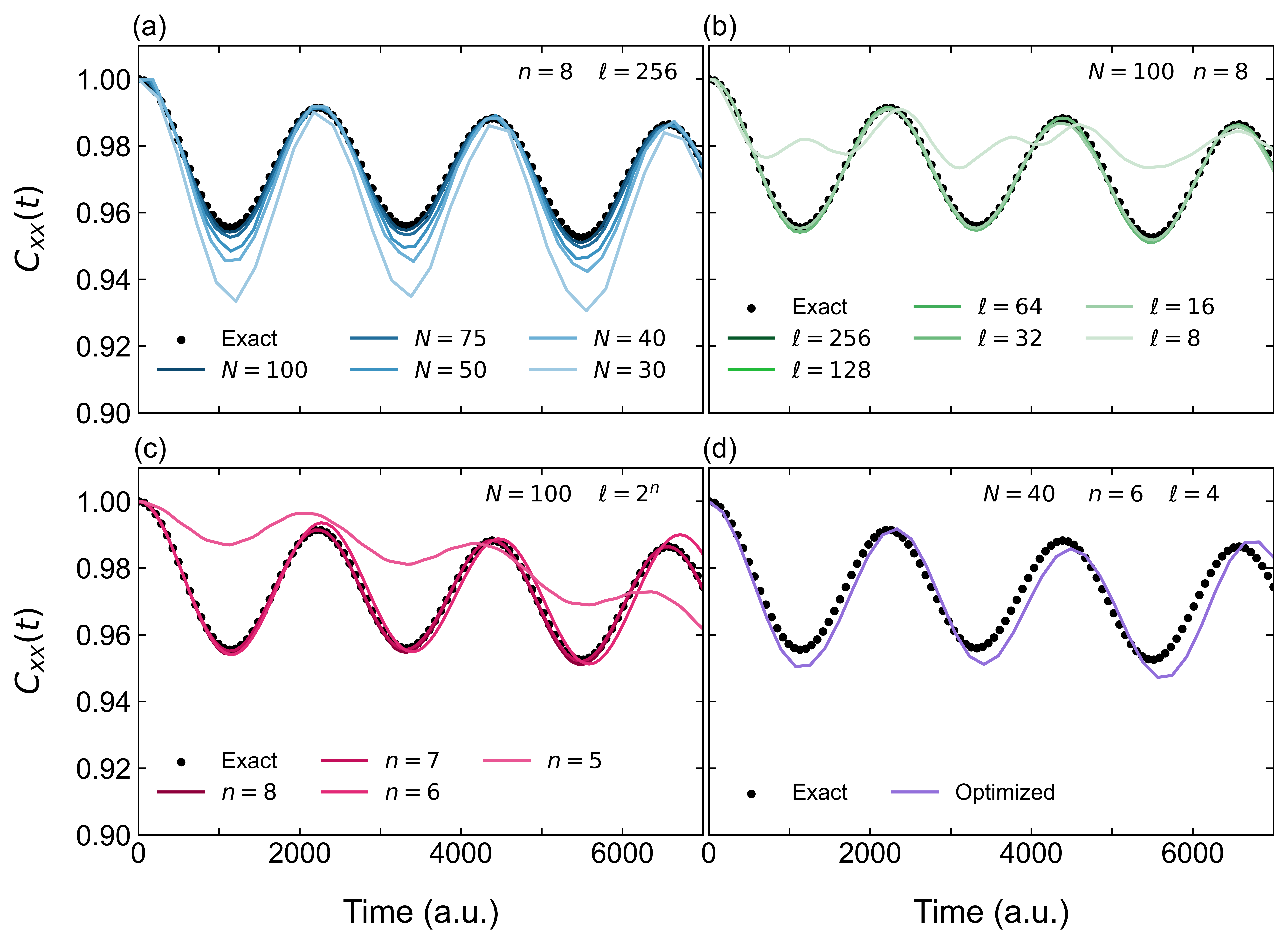
Initially, we used Eq. (30) to approximate evolution under the kinetic energy operator for both real- and imaginary-time. However, we found that the value of needed to achieve reasonable error was too large for PIMC methods. Instead, we found that using Eq. (30) for imaginary-time only, and using a standard Quantum Fourier Transform (QFT) approach to diagonalize the kinetic energy operator in real-time yielded better results. The results presented in Fig. 1 were obtained using this approach. Interestingly, we also found that using QFT for both real- and imaginary-time evolution yielded worse results than using Eq. (30) for both, and that the results do not systematically improve with increasing as one would expect.
In Fig. 1, panel , we see that for sufficiently large the approximate results match the exact results. As decreases, the error from Trotter splitting increases, and we see the amplitude of the TCF begins to deteriorate, although the frequency of the oscillations remains accurate. In panel , we compare approximate and exact results for different numbers of grid points, . For and , the difference between them is indistinguishable. At , the approximate results deviate slightly, and for the grid spacing becomes too large and all features of the TCF are lost. In panel , we further approximate by neglecting all diagonals , where , from . We see that the approximate results lie directly on top of the exact results up to . In other words, of the diagonals in can be neglected without impacting the results of the calculation. This is important because each additionally neglected diagonal results in a shallower circuit. Finally, we see in panel (d) that our method of computing the TEO matrix elements is robust to the cumulative error resulting from varying multiple parameters simultaneously. These results are encouraging and demonstrate that evolution under the kinetic energy operator can be well approximated by directly exponentiating , and that the Trotter error inherent in Eq. (30) and introduced through PITE is manageable for . Further, only qubits and diagonals are needed to achieve sufficient accuracy to simulate a proton transfer model.
In this initial paper, we proposed and developed the theory of hPIMC. We showed that hPIMC is ideally suited for condensed phase systems and could enable the study of higher-dimensional systems that are currently inaccessible through classical algorithms. How hPIMC performs in practice is a future direction that we will pursue. We also proposed a quantum algorithm for computing evolution under the kinetic energy operator in position space using a DVR approximation and demonstrated its practicality by computing the TCF of a proton transfer reaction. Finally, the work described here represents a new direction in solving NISQ era quantum dynamics problems.
VI acknowledgments
The authors thank Peter McMahon for insightful discussion and guidance.
References
- Preskill [2018] J. Preskill, Quantum Computing in the NISQ era and beyond, Quantum 2, 79 (2018).
- McClean et al. [2016] J. R. McClean, J. Romero, R. Babbush, and A. Aspuru-Guzik, The theory of variational hybrid quantum-classical algorithms, New J. Phys. 18, 023023 (2016).
- Miessen et al. [2021] A. Miessen, P. J. Ollitrault, and I. Tavernelli, Quantum algorithms for quantum dynamics: A performance study on the spin-boson model, Phys. Rev. Research 3, 043212 (2021).
- Ollitrault et al. [2020] P. J. Ollitrault, G. Mazzola, and I. Tavernelli, Nonadiabatic Molecular Quantum Dynamics with Quantum Computers, Phys. Rev. Lett. 125, 260511 (2020).
- Ollitrault et al. [2021] P. J. Ollitrault, A. Miessen, and I. Tavernelli, Molecular Quantum Dynamics: A Quantum Computing Perspective, Acc. Chem. Res. 54, 4229 (2021).
- Yung et al. [2014] M.-H. Yung, J. Casanova, A. Mezzacapo, J. McClean, L. Lamata, A. Aspuru-Guzik, and E. Solano, From transistor to trapped-ion computers for quantum chemistry, Sci. Rep. 4, 3589 (2014).
- Wang et al. [2019] D. Wang, O. Higgott, and S. Brierley, Accelerated Variational Quantum Eigensolver, Phys. Rev. Lett. 122, 140504 (2019).
- Peruzzo et al. [2014] A. Peruzzo, J. McClean, P. Shadbolt, M.-H. Yung, X.-Q. Zhou, P. J. Love, A. Aspuru-Guzik, and J. L. O’Brien, A variational eigenvalue solver on a photonic quantum processor, Nat. Commun. 5, 4213 (2014).
- Lee et al. [2022] C.-K. Lee, C.-Y. Hsieh, S. Zhang, and L. Shi, Variational Quantum Simulation of Chemical Dynamics with Quantum Computers, J. Chem. Theory Comput. 18, 2105 (2022).
- Yao et al. [2021] Y.-X. Yao, N. Gomes, F. Zhang, C.-Z. Wang, K.-M. Ho, T. Iadecola, and P. P. Orth, Adaptive Variational Quantum Dynamics Simulations, PRX Quantum 2, 030307 (2021).
- Xing et al. [2023] X. Xing, A. Gomez Cadavid, A. F. Izmaylov, and T. V. Tscherbul, A hybrid quantum-classical algorithm for multichannel quantum scattering of atoms and molecules, J. Phys. Chem. Lett 14, 6224 (2023).
- Wang et al. [2021] S. Wang, E. Fontana, M. Cerezo, K. Sharma, A. Sone, L. Cincio, and P. J. Coles, Noise-induced barren plateaus in variational quantum algorithms, Nat. Commun. 12, 6961 (2021).
- Sack et al. [2022] S. H. Sack, R. A. Medina, A. A. Michailidis, R. Kueng, and M. Serbyn, Avoiding Barren Plateaus Using Classical Shadows, PRX Quantum 3, 020365 (2022).
- Cerezo et al. [2021] M. Cerezo, A. Arrasmith, R. Babbush, S. C. Benjamin, S. Endo, K. Fujii, J. R. McClean, K. Mitarai, X. Yuan, L. Cincio, and P. J. Coles, Variational quantum algorithms, Nat. Rev. Phys. 3, 625 (2021).
- Layden et al. [2023] D. Layden, G. Mazzola, R. V. Mishmash, M. Motta, P. Wocjan, J.-S. Kim, and S. Sheldon, Quantum-enhanced Markov chain Monte Carlo, Nature 619, 282 (2023).
- Makri [1998] N. Makri, Quantum Dissipative Dynamics: A Numerically Exact Methodology, J. Phys. Chem. A 102, 4414 (1998).
- Topaler and Makri [1992] M. Topaler and N. Makri, Multidimensional path integral calculations with quasiadiabatic propagators: Quantum dynamics of vibrational relaxation in linear hydrocarbon chains, J. Chem. Phys. 97, 9001 (1992).
- Topaler and Makri [1993a] M. Topaler and N. Makri, Quasi-adiabatic propagator path integral methods. Exact quantum rate constants for condensed phase reactions, Chem. Phys. Lett. 210 (1993a).
- Topaler and Makri [1993b] M. Topaler and N. Makri, System-specific discrete variable representations for path integral calculations with quasi-adiabatic propagators, Chem. Phys. Lett. 210, 448 (1993b).
- Topaler and Makri [1994] M. Topaler and N. Makri, Quantum rates for a double well coupled to a dissipative bath: Accurate path integral results and comparison with approximate theories, J. Chem. Phys. 101, 7500 (1994).
- Feynman [1982] R. P. Feynman, Simulating physics with computers, Int. J. Theor. Phys. 21, 467 (1982).
- Kosugi et al. [2022] T. Kosugi, Y. Nishiya, H. Nishi, and Y.-i. Matsushita, Imaginary-time evolution using forward and backward real-time evolution with a single ancilla: First-quantized eigensolver algorithm for quantum chemistry, Phys. Rev. Res. 4, 033121 (2022).
- Nishi et al. [2023] H. Nishi, K. Hamada, Y. Nishiya, T. Kosugi, and Y.-i. Matsushita, Optimal scheduling in probabilistic imaginary-time evolution on a quantum computer, Phys. Rev. Res. 5, 043048 (2023).
- Light and Carrington JR. [2000] J. C. Light and T. Carrington JR., Discrete-Variable Representations and their Utilization, Adv. Chem. Phys. 114 (2000).
- Littlejohn et al. [2002] R. G. Littlejohn, M. Cargo, T. Carrington, K. A. Mitchell, and B. Poirier, A general framework for discrete variable representation basis sets, J. Chem. Phys. 116, 8691 (2002).
- Colbert and Miller [1992] D. T. Colbert and W. H. Miller, A novel discrete variable representation for quantum mechanical reactive scattering via the S -matrix Kohn method, J. Chem. Phys. 96 (1992).
- Caratzoulas and Pechukas [1996] S. Caratzoulas and P. Pechukas, Phase space path integrals in Monte Carlo quantum dynamics, J. Chem. Phys. 104, 6265 (1996).
- Berry et al. [2007] D. W. Berry, G. Ahokas, R. Cleve, and B. C. Sanders, Efficient Quantum Algorithms for Simulating Sparse Hamiltonians, Commun. Math. Phys. 270, 359 (2007).
- Cao et al. [2019] Y. Cao, J. Romero, J. P. Olson, M. Degroote, P. D. Johnson, M. Kieferová, I. D. Kivlichan, T. Menke, B. Peropadre, N. P. D. Sawaya, S. Sim, L. Veis, and A. Aspuru-Guzik, Quantum Chemistry in the Age of Quantum Computing, Chem. Rev. 119, 10856 (2019).
- Babbush et al. [2018] R. Babbush, N. Wiebe, J. McClean, J. McClain, H. Neven, and G. K.-L. Chan, Low-Depth Quantum Simulation of Materials, Phys. Rev. X. 8, 011044 (2018).
- Su et al. [2021] Y. Su, D. W. Berry, N. Wiebe, N. Rubin, and R. Babbush, Fault-Tolerant Quantum Simulations of Chemistry in First Quantization, PRX Quantum 2, 040332 (2021).
- Babbush et al. [2019] R. Babbush, D. W. Berry, J. R. McClean, and H. Neven, Quantum simulation of chemistry with sublinear scaling in basis size, npj Quantum Inf. 5, 92 (2019).
- [33] A. M. Childs, J. Leng, T. Li, J.-P. Liu, and C. Zhang, Quantum simulation of real-space dynamics, arXiv:2203.17006 .
- Kassal et al. [2008] I. Kassal, S. P. Jordan, P. J. Love, M. Mohseni, and A. Aspuru-Guzik, Polynomial-time quantum algorithm for the simulation of chemical dynamics, Proc. Natl. Acad. Sci. 105, 18681 (2008).
- Allen et al. [2016] T. C. Allen, P. L. Walters, and N. Makri, Direct computation of influence functional coefficients from numerical correlation functions, J. Chem. Theory Comput. 12, 4169 (2016).
- Beneti and Strini [2008] G. Beneti and G. Strini, Quantum simulation of the single-particle Schrodinger equation, Am. J. Phys. 76, 657–662 (2008).
- Aharonov et al. [2009] D. Aharonov, V. Jones, and Z. Landau, A polynomial quantum algorithm for approximating the jones polynomial, Algorithmica 55, 395 (2009).
- Trotter [1959] H. F. Trotter, On the product of semi-groups of operators, Proceedings of the American Mathematical Society 10, 545 (1959).
- Aharonov and Ta-Shma [2003] D. Aharonov and A. Ta-Shma, Adiabatic quantum state generation and statistical zero knowledge, in Proceedings of the Thirty-Fifth Annual ACM Symposium on Theory of Computing (2003) p. 20–29.
- Childs et al. [2003] A. M. Childs, R. Cleve, E. Deotto, E. Farhi, S. Gutmann, and D. A. Spielman, Exponential algorithmic speedup by a quantum walk, in Proceedings of the Thirty-Fifth Annual ACM Symposium on Theory of Computing (Association for Computing Machinery, New York, NY, USA, 2003) p. 59–68.
VII Supplemental Materials
VII.1 I. Bounding Thermal Correlation Function Error
In this section we prove that the error made from approximating the TCF using can be bound by
| (32) |
where is the matrix 1-norm or trace norm, and we assume that . We start by defining the error as , where is the TCF approximated by . Taking the difference and using that the trace is linear gives
| (33) | ||||
Using that is sub-multiplicative and sub-linear, we find
| (34) | ||||
where we use that . Proceeding,
| (35) | ||||
where the last line follows from splitting and into a product of real and imaginary time evolution operators and recognizing that the real time contributions cancel in . We arrive at our final result by keeping only terms first order in ,
| (36) |
VII.2 II. Bounding DVR Approximation Error
Here, we prove bounds on the error between the exact one-dimensional DVR kinetic energy matrix and an approximation in which a set of diagonals are neglected. We start by assigning to each diagonal of an index, , such that the main diagonal is , the adjacent upper and lower diagonals are , and so on. Let be an approximation to such that all diagonals are neglected. We define the error between and as
| (37) |
where and is the matrix 2-norm or Frobenius norm. Computing the trace and using the fact that is real and symmetric gives
| (38) |
where the sum runs over each diagonal of the upper triangular block. The only diagonals of with non-zero elements are when . Combining this fact with the definition
| (39) |
yields
| (40) |
where and we have dropped the term since it only contributes when . As this corresponds to approximating as a matrix of zeros, it is physically unmeaningful.
VII.3 A. Error Upper Bound
We now prove that the error is upper bound by . To do this, we first prove that is upper bound by . Note that is equivalent to the area comprised by a set of rectangles with heights centered at and edges specified by the points and . This area will always be less than
| (41) |
where the first term gives the area of the rectangle for . The integral gives the area of the remaining terms and will always be larger than the associated sum because we shift the integrand to the right by so that it intersects the right corner of each rectangle rather than its midpoint. Because the first term covers the domain , the integral runs from . In the limit of large and upon integration, the difference between the upper bound and becomes
| (42) |
Because the positive terms on the RHS are monotonically increasing in magnitude and the negative terms are monotonically decreasing in magnitude, if the expression is greater than zero for a given , it must also be greater than zero for all larger . For , we find . This completes the proof.
We arrive at our final expression for the error upper bound by taking the square root,
| (43) | ||||
VII.4 B. Error Lower Bound
We now prove that the error is lower bound by . To do this, we first prove that . This can be seen by showing that the sum of the first three terms of is always larger than . When the remaining terms are included in , the inequality still holds because each term is positive. To show that the first three terms of are always larger than , we take the difference between them and note that after expanding, all positive terms are monotonically increasing in magnitude while all negative terms are monotonically decreasing in magnitude. Following the same logic as for the error upper bound proof, we substitute into the expression and find that it yields a positive number, proving the lower bound. Note that must be true for this argument to hold. Finally, taking the square root yields
| (44) |
VII.5 C. Error Bound Comparison
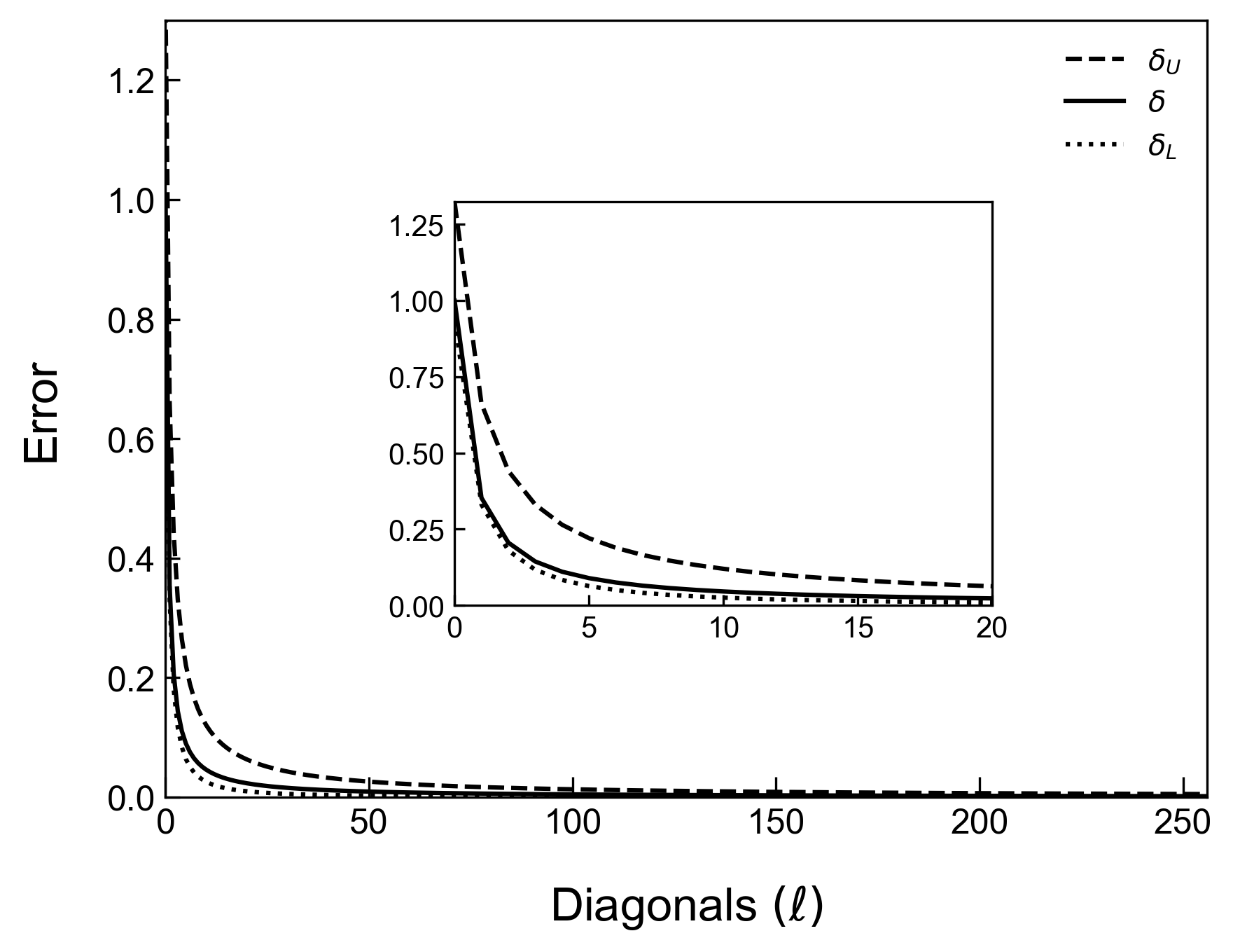
In Fig. 2 we compare the exact error of approximating , given by , with the upper and lower bounds derived above. We can see from Fig. 2 that the lower bound closely approximates the exact error and does a better job doing so than the upper bound. For this reason and because Eq. (44) is easier to work with and gives more insight than Eq. (40), we take the error lower bound as our expression for the error of approximating .
VII.6 III. 1-Sparse Decomposition
In this section we prove that any matrix can be decomposed into a sum of at most two 1-sparse, Hermitian matrices. Here, returns the input matrix with all elements neglected except those on the th upper and lower diagonals. A matrix is said to be -sparse if each row and column have at most elements. Thus, a -sparse matrix has at most one element in every row and column. We note that because consists of at most two diagonals (except , which is the main diagonal), then is at most -sparse. Additionally, is always Hermitian since is Hermitian as well.
Let and be the list of pairs of indices corresponding to the upper and lower diagonals of , respectively. For example, , where and are the row and column index, respectively, and is defined similarly. Given and , we can determine if is -sparse by checking that none of the row indices in are the same as and that none of the column indices in are the same as . If this is true, then is -sparse.
Case 1, : This is automatically -sparse and Hermitian as corresponds to the main diagonal.
Case 2, : This is automatically -sparse and Hermitian as well. To see this, note that the th index pair of and are given by and , respectively. We can write with . Plugging this into the index pairs, we find and . For a given , ranges from . From this, we can see that all column indices in the upper and lower diagonals will never be the same. This is also true for all row indices. Thus, is -sparse. Hermiticity follows form being Hermitian.
Case 3a, and is even: Here, each is -sparse and can be decomposed into a sum of two -sparse matrices in the following way. Starting from the leftmost element of the upper and lower diagonals, group this pair into a matrix, . Group the adjacent element to the right of the upper and lower diagonals into a matrix, . Continue alternating between grouping pairs into and until all pairs have been grouped. Both and are -sparse and Hermitian, and the sum of both matrices is .
To see this, we write where is even and . Inserting this into the index pairs we find and . Note that all pairs where is odd are grouped into . Then, because must be even, the opposite index will always be even as well. That is, and . Because the row indices in the upper and lower diagonals are always odd and even, respectively, they can never be the same. Similarly, because the column indices in the upper and lower diagonals are always even and odd, respectively, they too can never be the same. Hence, is -sparse.
All index pairs where is even are grouped into . Here, the opposite index is always odd. That is, and . Following the same logic as for , we see that is also -sparse. Because and are both symmetric and all matrix elements are the same, they are both Hermitian as well.
Case 3b, and is odd: Here, each is -sparse and can be decomposed into a sum of two -sparse matrices in the following way. Let and be a pair of positive integers such that
| (45) |
and is odd. We note that such a pair can be shown to always exist and be unique. Starting from the leftmost element of the upper and lower diagonals, partition the matrix into sets of contiguous elements. Then, starting from the leftmost set of both upper and lower diagonals, group every other set into a matrix, . Group all remaining sets into another matrix, . Both and are -sparse and Hermitian, and the sum of both matrices is .
To see this, we assign each set of contiguous elements an integer index where and . Assign the leftmost set . Moving to the right, assign the adjacent set . Continue assigning indices in this way until the rightmost set is reached. For , the upper diagonal row indices and lower diagonal column indices of the th set of contiguous elements range from while the upper diagonal column indices and lower diagonal row indices of the th set of contiguous elements range from . Note that is always odd for . Using the relationship gives for the range of upper diagonal column indices and lower diagonal row indices. We summarize this in Table 1 below.
| row indices | column indices | |
|---|---|---|
| upper diagonal | ||
| lower diagonal |
Consider the range of row indices for both upper and lower diagonals. Because is always even and is always odd, the range of row indices will never overlap for any given . We can see this immediately holds for the range of column indices as well. Thus, is -sparse. We can see that is -sparse by repeating the same steps as for and noting that the only difference is that is now even. The sum of both and is . Because and are both symmetric and all matrix elements are the same, they are both Hermitian as well. This completes the proof.