Ground state phases of the two-dimension electron gas with a unified variational approach

Abstract

The two-dimensional electron gas (2DEG) is a fundamental model, which is drawing increasing interest because of recent advances in experimental and theoretical studies of 2D materials. Current understanding of the ground state of the 2DEG relies on quantum Monte Carlo calculations, based on variational comparisons of different ansatze for different phases. We use a single variational ansatz, a general backflow-type wave function using a message-passing neural quantum state architecture, for a unified description across the entire density range. The variational optimization consistently leads to lower ground-state energies than previous best results. Transition into a Wigner crystal (WC) phase occurs automatically at $r_{s}=37\pm 1$, a density lower than currently believed. Between the liquid and WC phases, the same ansatz and variational search strongly suggest the existence of intermediate states in a broad range of densities, with enhanced short-range nematic spin correlations.

The uniform electron gas, also known as jellium, has been one of the most important fundamental models in condensed matter physics. The ground-state energies computed in jellium Ceperley and Alder (1980); Tanatar and Ceperley (1989); Attaccalite et al. (2002); Drummond and Needs (2009) also serve as the foundation for density functionals which are widely applied in ab initio computations in many disciplines. Recently the two-dimensional electron gas (2DEG) has drawn renewed interest owing to the many recent experimental discoveries in two-dimensional materials Hossain et al. (2020, 2021, 2022); Smoleński et al. (2021); Falson et al. (2022). Despite the simplicity of the model, the phase diagram of jellium is not fully understood. Theoretically, a variety of candidate ground states have been proposed Falakshahi and Waintal (2005), including theory of microemulsion Spivak and Kivelson (2004) and metalic electron crystal Kim et al. (2023) between phase transitions. Computationally, the most accurate studies have confirmed only a Fermi liquid (FL) phase at high density, and a Wigner crystal (WC) phase (possibly with different spin polarizations) at low density, with a transition between them estimated at $r_{s}=31\pm 1$ in two dimensions, based on the most accurate computations to date Drummond and Needs (2009). Experimentally, generalized WC phases, in the presence of external potentials, have been detected Li et al. (2021); Shabani et al. (2021); Regan et al. (2020), and higher density regimes are being realized and studied. In particular, a low-temperature magneto-optical experiment in MoSe₂ Sung et al. (2023) reported evidence for a liquid phase with enhanced spin susceptibility and a microemulsion phase in between the WC and the FL.

The primary challenge in computationally determining the ground-state phases in jellium is that candidate states are separated by extremely small energy differences. In order to make further progress, we need methods that have systematically improvable and, possibly more importantly, balanced accuracy across different regimes. Quantum Monte Carlo calculations have been the standard tool used so far. However, they typically rely on different variational ansatze for different phases. The ground state at each density is determined by comparing the computed energies from each candidate ansatz, and the search for different states is limited by the expressiveness of the variational ansatze that can be computed given the available resources.

Recently, neural network wavefunctions Carleo and Troyer (2017); Pfau et al. (2020); Hermann et al. (2020, 2023), also known as neural quantum states (NQS), have been used as ansatze in variational Monte Carlo (VMC) calculations. They significantly expand the expressiveness of the variational wave functions that can be explored and computed. Many developments and applications have shown the promise of this approach. Impressive accuracy has been achieved in a variety of benchmark studies in fermion systems. However, to date, few applications in this area have demonstrated the potential predictive power that can lead to physical results or insights beyond the reach of existing capabilities.

In this paper, we leverage NQS to study the ground state phases of the 2DEG. We uncover evidence of short-range nematic spin correlations in a broad range of intermediate densities, and automatically discover a “floating” WC. Building on an ansatz of Slater-Jastrow-backflow form with message-passing graph neural network components Pescia et al. (2022), we introduce multiple planewaves (MPs) into each orbital, allowing the ansatz to span both the liquid and WC phases. Using this single ansatz, which we call (MP)²NQS, we obtain variational ground-state energies significantly lower than those from state-of-the-art QMC Drummond and Needs (2009). The transition to the WC is automatic, yielding a lower critical density ($r_{s}=37\pm 1$) than previously believed. In the WC phase, the ansatz yields a “floating” crystal with partially restored translational symmetry. With the same ansatz, our calculations suggest the existence of an intermediate state in a wide range of densities ($r_{s}\sim 10$-$35$) before the WC transition, a liquid state with enhanced short-range spin correlations which break rotational symmetry. Although the calculations are still in modest system sizes (but comparable to the largest sizes that have been treated by NQS), our analysis indicates that the nematic spin correlation is quite robust, and that the 2DEG may have much new physics to offer.

The 2DEG consists of interacting electrons in a uniform compensating charge background. The Hamiltonian (in Hartree atomic units)

$$H=-\dfrac{1}{2}\sum\limits_{i}\nabla_{i}^{2}+\sum\limits_{i<j}\dfrac{1}{|\boldsymbol{r}_{i}-\boldsymbol{r}_{j}|}+{\rm b.g.}$$ (1)

is specified by a single dimensionless parameter, $r_{s}$, the Wigner-Seitz radius in units of the Bohr radius $a_{\mathrm{B}}$ (see considerations of a finite simulation with periodic boundary conditions in SM). Our (MP)²NQS ansatz has Slater-Jastrow-backflow form

$$\Psi(R)=\text{det}\left[\{\langle\boldsymbol{x}_{j};\sigma_{j}|\phi_{a};\chi_{a}\rangle\}\right]\exp\big(U_{2}(R)+\mathcal{U}(R)\big{missing})\,,$$ (2)

where $R\equiv\{\boldsymbol{r}_{1};\sigma_{1};\boldsymbol{r}_{2};\sigma_{2};\cdots;\boldsymbol{r}_{N};\sigma_{N}\}$ denotes the coordinates and spins of the $N$ electrons in the simulation cell of area $\Omega$ ($\pi r_{s}^{2}=\Omega/N$), and the “quasi-particle” coordinates are

$$\boldsymbol{x}_{j}\equiv\boldsymbol{r}_{j}+\mathcal{N}(R)\,.$$ (3)

Both $\mathcal{N}$ in Eq. (3) and $\mathcal{U}$ in the Jastrow in Eq. (2) are many-body neural network functions, inspired by the message-passing neural quantum states (MP-NQS) ansatz Pescia et al. (2023). In this work, we restrict the system to total $S_{z}=0$, and each $\sigma_{j}$ is fixed ($+1$ or $-1$). We also keep each orbital $\chi_{a}$ as an $\hat{s}_{z}$ eigenstate. (This reduces the Slater determinant to a product of separate spin-$\uparrow$ and spin-$\downarrow$ components.) Each of the $N$ orbitals in the Slater determinant can be written as

$$\phi_{a}(\boldsymbol{x})=\sum_{k=1}^{N_{k}}c_{ak}\exp(\mathrm{i}\boldsymbol{G}_{k}\cdot\boldsymbol{x})\,$$ (4)

where $\{c_{ak}\}$ are variational parameters and we choose $N_{k}\gg N$ (multiple planewaves). The function $U_{2}$ in Eq. (2) is a sum of isotropic two-body correlators: $U_{2}(R)=\sum_{j\neq l}u_{\sigma_{j}\sigma_{l}}(\boldsymbol{x}_{j}-\boldsymbol{x}_{l})$ , where $u_{+1}$ and $u_{-1}$ are standard functions satisfying the cusp condition for same and opposite spins, respectively Ceperley et al. (1977).

While the original idea of backflow was based on physical intuition from liquid helium Feynman (1954); Feynman and Cohen (1956) and perturbation theory Kwon et al. (1993); Holzmann et al. (2003); Taddei et al. (2015), recent implementations Ruggeri et al. (2018); Pfau et al. (2020); Cassella et al. (2023); Pescia et al. (2022); Wilson et al. (2023) parameterize a general all-body, instead of few-body, coordinate transformation. In this work, we adapt the message passing network from Pescia et al. (2023) as our many-body backflow transformation $\mathcal{N}(R)$, with modifications to facilitate optimization. We introduce an extra term $\mathcal{U}(R)$ in the Jastrow factor that shares the same message-passing layers with the backflow $\mathcal{N}$, to further improve the expressivity of the ansatz. Details of our implementation can be found in the Supplementary Materials.

We variationally minimize the total energy

$$E=\frac{\int[H\Psi(R)/\Psi(R)]\,|\Psi(R)|^{2}\,dR}{\int|\Psi(R)|^{2}\,dR}\,.$$ (5)

The Metropolis-adjusted Langevin algorithm (MALA)  Besag (1994) is employed to sample electron configurations $\{R\}$ from the unnormalized distribution $|\Psi(R)|^{2}$, which allows the evaluation of Eq. (5) as the expectation of the local energy: $\mathbb{E}[H\Psi(R)/\Psi(R)]$. New configurations in the Markov chain are proposed using overdamped Langevin dynamics, which utilizes gradient information to increase the acceptance rate. The step size of the Langevin dynamics is adaptively tuned during the optimization according to the average acceptance rate. The optimization of the parameters is performed using the stochastic reconfiguration (SR) method Sorella (1998, 2005) with recently introduced modifications Goldshlager et al. (2024) to stabilize and accelerate the process.

We apply the same ansatz and optimization procedure to different $r_{s}$ values spanning both liquid and crystal phases. The hyperparameters used for different $r_{s}$ values are the same, except for the initial learning rates, which are tuned for each $r_{s}$ to account for the different energy scales. The calculations are primarily carried out with $N=56$ electrons under periodic boundary conditions, with spot checks using $N=58$ (square simulation cell) and $N=120$.

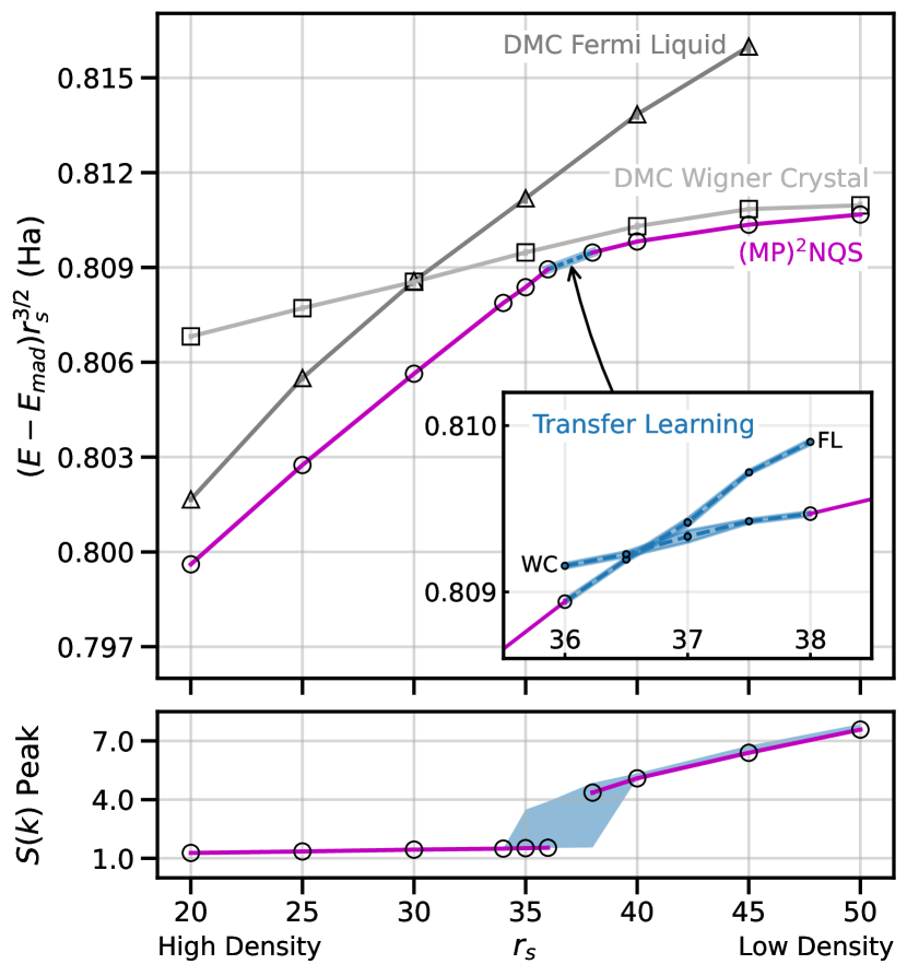
Figure 1: Accurate and automatic detection of the Wigner crystal transition. The ground-state energies from variational optimization of the unified (MP)²NQS ansatz systematically outperform state-of-the-art results from diffusion Monte Carlo (DMC) using separate variational ansatze as trial wave functions (top panel). Statistical error of energies from the (MP)²NQS ansatz is smaller than the line width. The inset shows a study near the WC transition using transfer learning, which preserves the character of the state while changing its density. The bottom panel shows the Bragg peak values in the static structure factor $S(\boldsymbol{k})$ calculated from (MP)²NQS. The shaded region indicate uncertainty from the optimization process as discussed in the main text. Results here are obtained from simulation cells containing $N=56$ electrons.

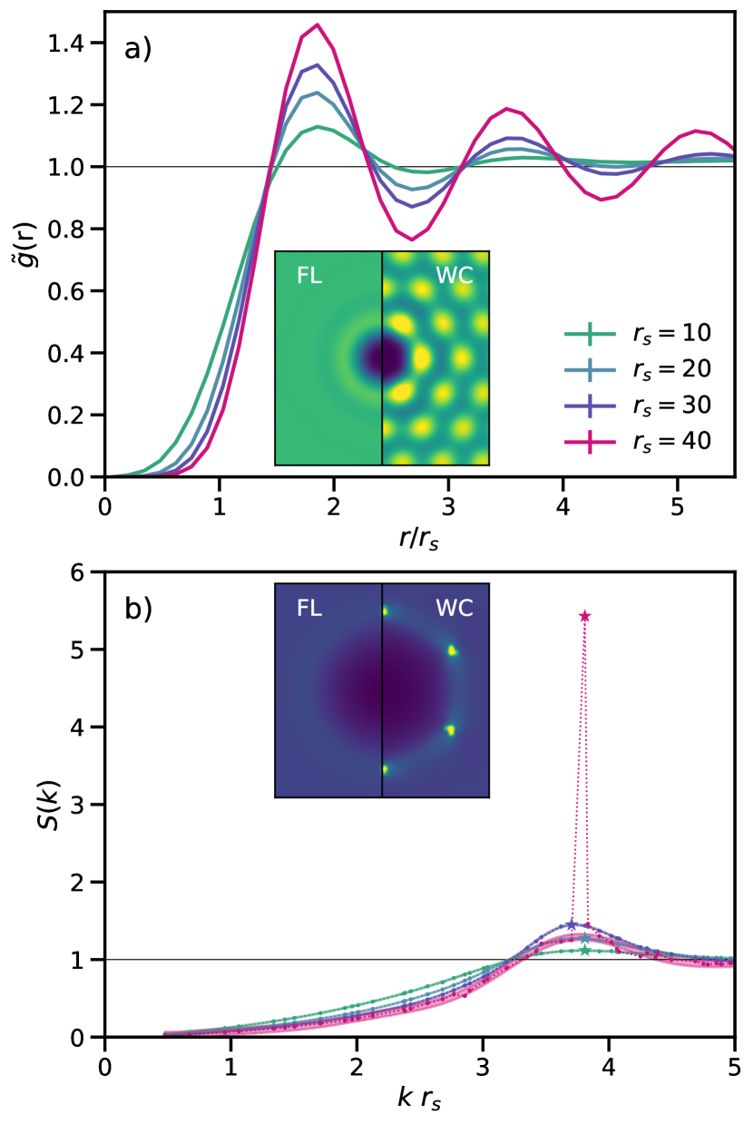
Figure 2: Charge-charge correlations for representative densities, shown as (a) the pair correlation function $\tilde{g}(\boldsymbol{r})$, and (b) the static structure factor $S(\boldsymbol{k})$. The main panels show the radially averaged quantities, while the insets show the full two dimensional versions. Each inset is divided into two halves, with the left showing $r_{s}=10$ and the right showing $r_{s}=40$. At $r_{s}=40$, long-range correlation is evident from the persistent oscillations in the tail of $\tilde{g}(r)$ and the corresponding Bragg peak (pink star) in $S(k)$. Results shown in the insets are from $N=120$.

The (MP)²NQS ansatz automatically and accurately discovers the WC transition by variational optimization. Our current knowledge of this transition is based on diffusion Monte Carlo (DMC) calculations using different VMC ansatze, as shown in Fig. 1. The reference DMC calculations dmc are performed in identical systems as in the (MP)²NQS calculations and obtained with Slater-Jastrow-backflow trial wavefunctions with short-range isotropic two-body correlators, using planewaves for the FL phase and Gaussians for the WC phase.

The optimized variational energy from our neural network ansatz yields a single equation of state line shown in the main plot in Fig. 1, which is lower than that of DMC at all densities. The difference in energies is especially prominent in the liquid phase. In the bottom panel of Fig. 1, we can see the crystallinity of the (MP)²NQS  ansatz spontaneously increase across the WC transition. Near the transition, in the range $r_{s}\in(34,40)$, the ansatz discovers states with and without charge order in a narrow energy window depending on the randomly generated initial parameters. The shaded region encapsulates results of all states having energy close to the lowest state (with a threshold of $0.01\%$ of the total energy). To locate the critical $r_{s}$ more precisely, we use the transfer learning technique to preserve the character (FL or WC) of the ansatz in the transition region and calculate its variational energy. As shown in the inset of Fig. 1, we transferred the liquid state found at $r_{s}=36$ up to $38$ and the crystal state found at $r_{s}=38$ down to $r_{s}=36$. The energy crossing gives a transition point of $r_{s}=36.5$. After applying finite-size corrections using energies from DMC Drummond and Needs (2009) (which is less costly to run for larger simulation sizes), we obtain an estimated critical value for the WC transition: $r_{s}=37\pm 1$.

The main advantage of the (MP)²NQS is that, within the same ansatz, correlated phases such as the WC can be automatically discovered. Further, once an NQS has been optimized, many physical observables can be calculated to high precision to characterize the discovered phase. DMC has been the standard for accurate characterization of ground-state properties in jellium. There have been years of sophisticated development and optimization since the early landmark calculation Ceperley and Alder (1980). That the variational energy is lower than DMC is important, not so much for the quantitative improvement, but as a strong indication of the quality of the (MP)²NQS wave function.

We next examine the properties of the (MP)²NQS ground state as a function of $r_{s}$. We compute spin-resolved one- and two-body density functions: $\rho_{\alpha}(\boldsymbol{r})=\langle\Psi|\hat{\rho}_{\alpha}(\boldsymbol{r})|\Psi\rangle$ and $\rho^{\alpha,\beta}_{2}(\boldsymbol{r},\boldsymbol{r}^{\prime})=\langle\Psi|\hat{\rho}_{\alpha}(\boldsymbol{r})\hat{\rho}_{\beta}(\boldsymbol{r}^{\prime})|\Psi\rangle$, where $\alpha$ and $\beta$ are spin indices ($\in\Bqty{\uparrow,\downarrow}$) and $\hat{\rho}_{\alpha}(\boldsymbol{r})$ is the density operator at $\boldsymbol{r}$ for spin $\alpha$. The uniform pair correlation function is

$$\tilde{g}(\boldsymbol{r})=\frac{\Omega}{N(N-1)}\int\differential{\boldsymbol{r}_{0}}\sum_{\alpha,\beta\in\{\uparrow,\downarrow\}}\rho^{\alpha,\beta}_{2}(\boldsymbol{r}_{0},\boldsymbol{r}_{0}+\boldsymbol{r})\,,$$ (6)

and the Fourier transform of $\tilde{g}(\boldsymbol{r})$ is the structure factor

$$S(\boldsymbol{k})= ~{}1+\frac{N-1}{\Omega}\int\differential{\boldsymbol{r}}e^{-\mathrm{i}\boldsymbol{k}\cdot\boldsymbol{r}}(\tilde{g}(\boldsymbol{r})-1)\,.$$ (7)

Figure 2(a) and (b) show $\tilde{g}(\boldsymbol{r})$ and $S(\boldsymbol{k})$ in direct and reciprocal space, respectively. At $r_{s}=40$, $\tilde{g}(r)$ shows strong and persistent oscillation at large distances, indicative of long-range correlation. Correspondingly, the $S(\boldsymbol{k})$ exhibits Bragg peaks at wave vectors consistent with a triangular WC. As shown in Fig. 2(b) and the bottom panel of Fig. 1, we find $S(\boldsymbol{k})$ is smooth vs. $k\equiv|\boldsymbol{k}|$ for $r_{s}\leq 34$, confirming the lack of long-range charge correlation, and the character of a liquid.

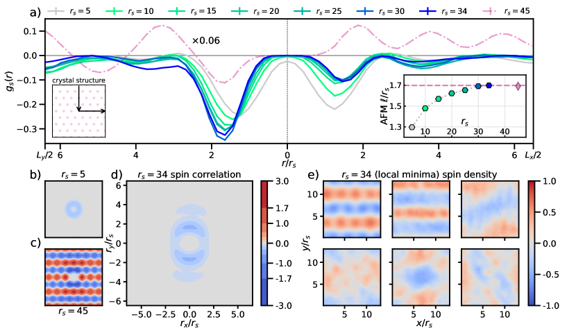
Figure 3: Signatures of the intermediate NSCL states. In (a), line cuts of the spin correlation function, $g_{s}(\boldsymbol{r})$, are shown scanning the densities between a prototypical liquid ($r_{s}=5$) and a WC ($r_{s}=45$). Significant short-range anisotropic spin correlations are present starting from $r_{s}\sim 10$. The anisotropy grows with $r_{s}$, with the nearest spin showing stronger (anti-parallel) correlation and drifting further toward the near-neighbor position in the WC, as shown in the inset, which plots the location of the first minimum position in the left half of the main panel, as a function of $r_{s}$. The 2D $g_{s}(\boldsymbol{r})$ of representative states are shown in (b) $r_{s}=5$, (c) $r_{s}=45$ and (d) $r_{s}=34$. At $r_{s}=34$, we found many local minima having total energy within $0.01$% of the lowest state. The spin densities of the six lowest-energy states are shown in (e), ordered by their energies starting with the lowest at top left, whose $g_{s}(\boldsymbol{r})$ is shown in (d), to the highest at bottom right of the panel.

The WC phase discovered by (MP)²NQS exhibits a partially floating nature, characterized by nearly uniform density along the spin stripes of an anti-ferromagnetic (AFM) pattern, as shown in appendix Fig. S3(d). (The broken symmetry spin stripe pattern is built into the ansatz, because we restrict it to colinear spins with fixed $\sigma_{j}$ and $\chi$ in Eq. (2).) This is different from the usual WC state studied computationally in the 2DEG, in which a WC is assumed and the electron locations in the crystal are specified a priori. This “floating crystal” state, despite being theoretically predicted long ago Bishop and Lührmann (1982); Lewin et al. (2019), has not been observed in numerical simulations reported in the literature to the best of our knowledge.

One of the long-standing questions on the electron gas is whether there are intermediate states between the FL and WC and, if so, of what character. The (MP)²NQS provides a unique opportunity to explore this question, given that the ansatz does not require postulating the candidate phases and that it is capable of high accuracy across the density regimes, as the results above indicate. Below, we investigate the ground state from (MP)²NQS more closely at the intermediate densities. We compute the spin-spin correlation function defined as

$$g_{s}(\boldsymbol{r})=\sum_{\alpha,\beta\in\{\uparrow,\downarrow\}}(2\delta_{\alpha\beta}-1)g_{\alpha\beta}(\boldsymbol{r}),$$ (8)

where $g_{\alpha\beta}(\boldsymbol{r})$ is the pair correlation function $\rho^{\alpha,\beta}_{2}(\boldsymbol{r}_{0},\boldsymbol{r}_{0}+\boldsymbol{r})/[\rho_{\alpha}(\boldsymbol{r}_{0})\rho_{\beta}(\boldsymbol{r}_{0}+\boldsymbol{r})]$ after averaging with respect to the reference position $\boldsymbol{r}_{0}$ (as done in Eq. (6)).

We find a strong tendency for short-range anisotropic spin correlations in a wide range of intermediate densities, which we will refer to below as nematic spin correlated liquid (NSCL, for short). In a typical liquid at $r_{s}=5$, $g_{s}(\boldsymbol{r})$ exhibits isotropic short-range AFM correlation due to exchange effects, as shown in Fig. 3(b) and the gray line in Fig. 3(a). In a typical crystal at $r_{s}=45$, $g_{s}(\boldsymbol{r})$ has long-range AFM correlation commensurate with the triangular lattice as shown in Fig. 3(c) (note stripe structure due to restricting to colinear spins, as discussed earlier) and the dot-dashed line in Fig. 3(a). As the interaction strength $r_{s}$ increases in the liquid phase, the spin channel develops nematic correlation while the charge channel remains isotropic (Fig. S4). The spin correlation remains very short-ranged until the WC is reached; however, starting from $r_{s}\sim 10$, a preferential AFM direction emerges. The AFM correlation strengthens along this direction and weakens perpendicular to it. With $N=56$, the simulation cell is rectangular, and almost all of the NSCL found here picked a direction within $10^{\circ}$ of the short axis. We have also verified with calculations in the $N=58$ square cell, where the AFM is equally likely to be along the $x$- or $y$-direction, and the $g_{s}(\boldsymbol{r})$ is quantitatively consistent with those in Fig. 3(a) (see appendix Figs. S2 and S6). By following the first dip in $g_{s}(r)$ along the preferred direction, which is aligned to $y$ in Fig. 3(a), we see that the characteristic length of this correlation increases from $\sim 1.5\,r_{s}$ at $r_{s}=10$ to $\sim 1.7\,r_{s}$ around the WC transition, as shown in the inset in panel a. This is consistent with the projection of the nearest neighbor distance in the WC along the $y$ direction (panel c). Therefore, the NSCL connects spin features of the liquid to that of the WC.

We also observed faint spin density stripes in the NSCL. As shown in Fig. 3(e), the six lowest-energy states found at $r_{s}=34$ (within $0.01\%$ in variational energy) all show some spin density wave order. The six states have spin densities, $s(\boldsymbol{r})\equiv\rho_{\uparrow}(\boldsymbol{r})-\rho_{\downarrow}(\boldsymbol{r})$, which vary in pattern, orientation, and strength. However they all have $g_{s}(\boldsymbol{r})$ nearly identical to Fig. 3(d), oriented in the direction of the AFM stripes. The spin density waves in the two lowest-energy states at $r_{s}=34$ have twice the wavelength of the WC. Strictly speaking, the broken symmetry in a one-body observable here is artificial, as we discussed earlier in connection with the partially floating crystals. We interpret these spin density waves as originating from the anisotropic two-body spin correlation, but pinned to a one-body density, possibly by a rough optimization landscape. The charge density remains nearly uniform in the NSCL (Fig. S3). At $r_{s}=34$, all the low-energy states we find are liquids. In contrast, at $r_{s}=35$, there are some local minima with WC character very close in energy to the lowest-energy state, which is a liquid (Fig. S1). Whether this can be a manifestation of microemulsion Spivak and Kivelson (2004) in the small simulation cells is an interesting question to explore. In principle, the current ansatz allows this and the possible existence of a metallic electronic crystal to be studied. As shown in Fig. 3(a), the short-range AFM feature is fully developed by $r_{s}=15$ and persists all the way up to crystallization. Interestingly, the density range coincides with the recent experimental observation Sung et al. (2023) of an intermediate liquid state with high spin susceptibility.

In summary, we report several advances in characterizing and understanding the ground state of the 2DEG, using a neural quantum state ansatz, (MP)²NQS. The single ansatz yields variational energies which are significantly lower than the current state-of-the-art from DMC projections of separately optimized VMC wave functions. It allows a unified description of the 2DEG, finding the FL and WC phases without any a priori specification, and revising the transition to the WC to a lower density than currently assumed. The same variational ansatz suggests the existence of a correlated liquid state with short-range nematic spin correlations at a wide range of intermediate densities. Further studies are needed, for example with more systematic investigation of finite-size effects and more extensive quantification of the different correlations and spin response, in order to better characterize these states and understand their connection with the experimental observations. But these results from the (MP)²NQS already provide evidence and interesting clue that there is rich physics between the FL and WC phases in the electron gas.

Note added: During the preparation of this manuscript, Azadi et al. Azadi et al. (2024) reported improved DMC calculations in the liquid phase, and a revised transition density of $r_{s}=35\pm 1$, more consistent with our result.

Acknowledgment.— The Flatiron Institute is a division of the Simons Foundation. The authors would like to thank David Ceperley, Eugene Demler, Ilya Esterlis, Gil Goldshlager, Andrew Millis, Vadim Oganesyan, Agnes Valenti, Han Wang, Lei Wang, Hao Xie, Linfeng Zhang for helpful discussions.

I Supplemental Materials:
Ground state phases of the two-dimension electron gas
with a unified variational approach

Conor Smith These authors contributed equally. Yixiao Chen These authors contributed equally.

Ryan Levy Yubo Yang Miguel A. Morales Shiwei Zhang

I.1 Total Energy and Static Structure Factor

In Table 1, we provide the lowest total energies and corresponding $S(k)$ Bragg peaks obtained using the (MP)²NQS ansatz along with total energies of reference DMC calculations. To emphasize the variation of final states from the frustrated optimization landscape, we show two figures of merit, the energy and averaged Bragg peaks of the structure factor $S(k)$, in Fig. S1. We find many competitive states in the region $r_{s}\in[34,40)$, depicted both in the energetics and the variety of $S(k)$ Bragg peak values. The lowest energy states in this regime are all liquid like until $r_{s}=38$, but the optimization may find a crystal or stripe state nearby in energy. Not pictured, there are non-crystalline states found at $r_{s}\geq 40$ but they are significantly higher than energy, a factor of approximately 3 higher. We note that the Wigner crystal states with slightly higher energies still show no signs of defects. They may have small modulations in the densities and are not as “floating” as the lowest energy ones.

Table 1: Total energy per electron $E/N$ in Hartree and average Bragg peak $S_{b}$ of $56$ electrons at various densities.

$r_{s}$	$E/N$	$S_{b}$		$E^{\mathrm{DMC}}_{\mathrm{FL}}/N$	$E^{\mathrm{DMC}}_{\mathrm{WC}}/N$
20	-0.04637(2)	1.273(7)		-0.046342(1)	-0.0462847(9)
25	-0.03782(1)	1.35(1)		-0.0378001(8)	-0.0377824(7)
30	-0.03197(1)	1.442(6)		-0.0319493(6)	-0.031949(1)
34	-0.028457(6)	1.493(6)
35	-0.027699(7)	1.519(8)		-0.0276854(8)	-0.0276936(5)
36	-0.026980(4)	1.539(5)
38	-0.025652(3)	4.4(1)
40	-0.024451(2)	5.1(1)		-0.0244356(7)	-0.0244496(4)
45	-0.021896(2)	6.39(8)		-0.0218769(7)	-0.0218940(3)
50	-0.019829(1)	7.58(6)			-0.0198283(3)

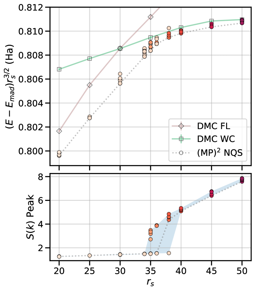
(a) Total energy and averaged $S(k)$ peak vs $r_{s}$.

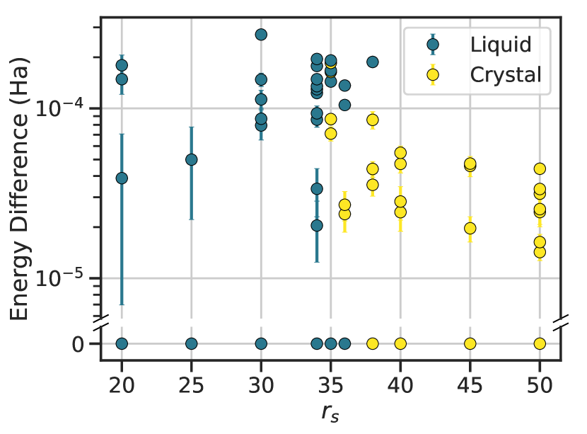
(b) Energy difference to the lowest obtained state vs $r_{s}$.

Figure S1: (a) Compiled optimization trials showing energy (top) and $S(k)$ peak (bottom) across different values of $r_{s}$. Grey open circles and a dotted line mark the lowest energy trials for a given density, while a lighter/darker color corresponds to a smaller/larger $S(k)$ peak. Shaded region corresponds to same of fig 1. (b) Energy difference to the lowest obtained state vs $r_{s}$. The different colors denote liquid states vs those that are WC.

I.2 Evolution of the AFM Correlations

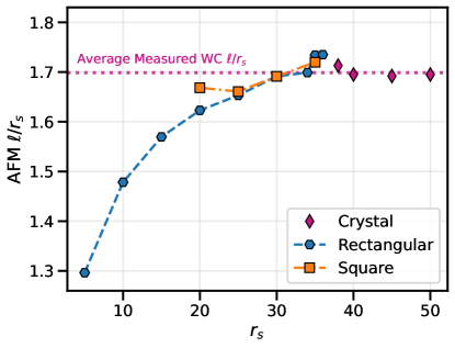
Figure S2: Fitted values of the peak location of $g_{s}(\boldsymbol{r})$ along the AFM direction as a function of $r_{s}$ for both rectangular and square cell of liquid phase and rectangular cell of crystal phase. The dotted horizontal line shows the averaged value of measured WC distance.

In Fig. S2, we explore the peak of the $g_{s}(\boldsymbol{r})$ location as a function of $r_{s}$ which was originally shown in the linecut of Fig. 3(c). The peak location roughly represents the distance between two pairs of opposite spin electrons, or the AFM characteristic length $\ell$. To obtain the peak location, we fit the underlying histogram data to a Gaussian

$$G(r,\theta;\{\ell,\theta_{i},\sigma_{r},\sigma_{\theta},A,B\})=A\exp\left(-\dfrac{(r-\ell)^{2}}{\sigma_{r}^{2}}-\dfrac{(\theta-\theta_{o})^{2}}{\sigma_{\theta}^{2}}\right)+B$$ (9)

to mitigate bias from finite grid resolution and statistical noise. As $r_{s}$ increases, the value of $\ell/r_{s}$ slowly climbs until $g_{s}(r)$ abruptly changes when the system becomes a WC at sufficiently large $r_{s}$.

We also measure the peak location of the triangular WC along the AFM direction (y axis in the simulation cell). The peak location is determined by a spline fit for the data on the grid along that axis. The average measured peak distance for WC is $\ell/r_{s}\approx 1.70$, as shown in the dotted horizontal line in Fig. S2. This value is slightly larger than what is predicted from a perfect triangular lattice, $\frac{\sqrt{3}}{2}\times\sqrt{\frac{2\pi}{\sqrt{3}}}\approx 1.65$, since the correlation function is distorted locally by the exchange effects.

We also note that the peak distance we get for $r_{s}=35$ and $36$ are slightly higher than the averaged crystal value, by around 2 %. One potential cause for this small overshoot is the frustrated optimization landscape, since we have multiple competing local minima of different phases within a small energy range at these two $r_{s}$ (see Fig. S1). Whether there is some physical explanation (such as microemulsion) behind this phenomenon is a direction to explore in the future.

I.3 Evolution of observables

We show in this section, for various $r_{s}$, charge and spin densities in Fig. S3, charge and spin correlation functions in Fig. S4, and momentum distributions

$$n(\boldsymbol{k})=\dfrac{1}{N(2\pi)^{2}}\int d\boldsymbol{r}_{0}\int d\boldsymbol{r}e^{-i\boldsymbol{k}\cdot\boldsymbol{r}}\rho_{2}(\boldsymbol{r}_{0},\boldsymbol{r}_{0}+\boldsymbol{r})$$ (10)

in Fig. S5. The charge density remains uniform in the liquid, whereas the spin density shows faint spin stripes in the NSCL states. The charge correlation remains isotropic in the liquid, where as the spin correlation shows short-range nematic AFM correlation in the NSCL states. The charge momentum distribution appears isotropic with a discontinuity at the Fermi surface $k=\sqrt{2}/r_{s}$ in the liquid. The magnitude of the discontinuity decreases as $r_{s}$ increases and disappears in the WC phase.

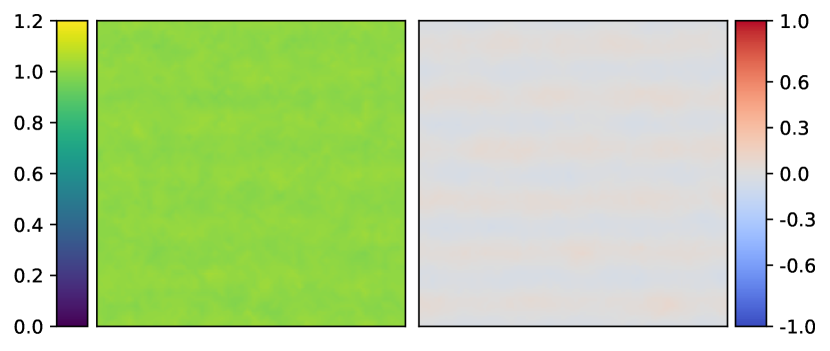
(a) $r_{s}=5$

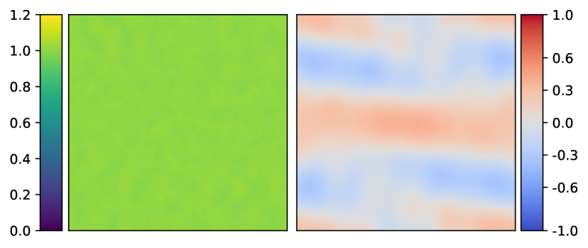
(b) $r_{s}=20$

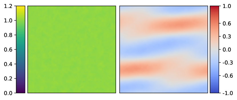
(c) $r_{s}=35$

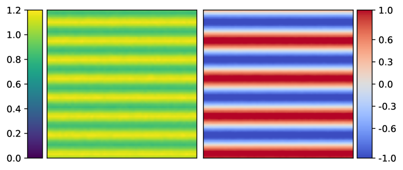
(d) $r_{s}=45$

Figure S3: Evolution of the charge (left) and spin (right) densities. We choose the normalization so that the charge density averages to one in the simulation cell.

(a) $r_{s}=5$

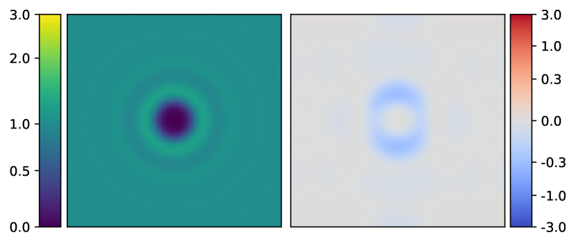
(b) $r_{s}=20$

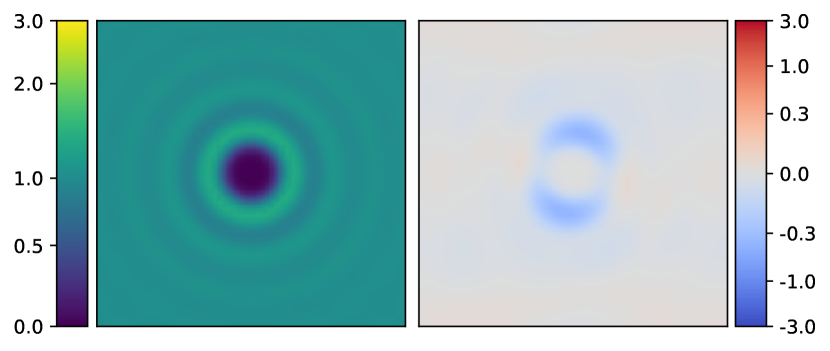
(c) $r_{s}=35$

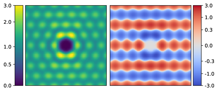
(d) $r_{s}=45$

Figure S4: Evolution of pair correlation functions $g(r)$ (left) and spin-spin correlation function $g_{s}(r)$ (right). Note the colorbar is nonuniform in order to capture different scales between liquid and crystal phases.

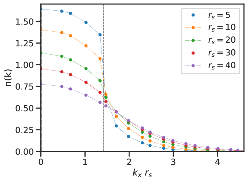
(a) radial average

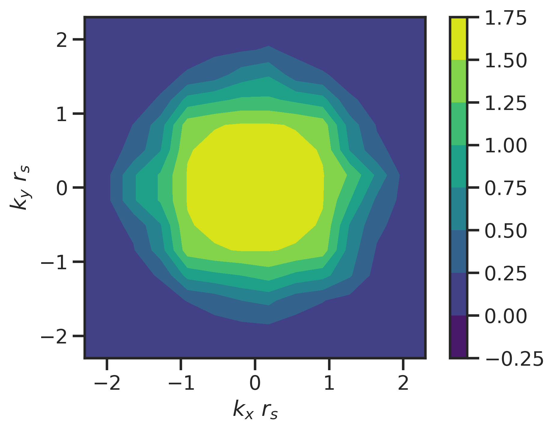
(b) $r_{s}=5$

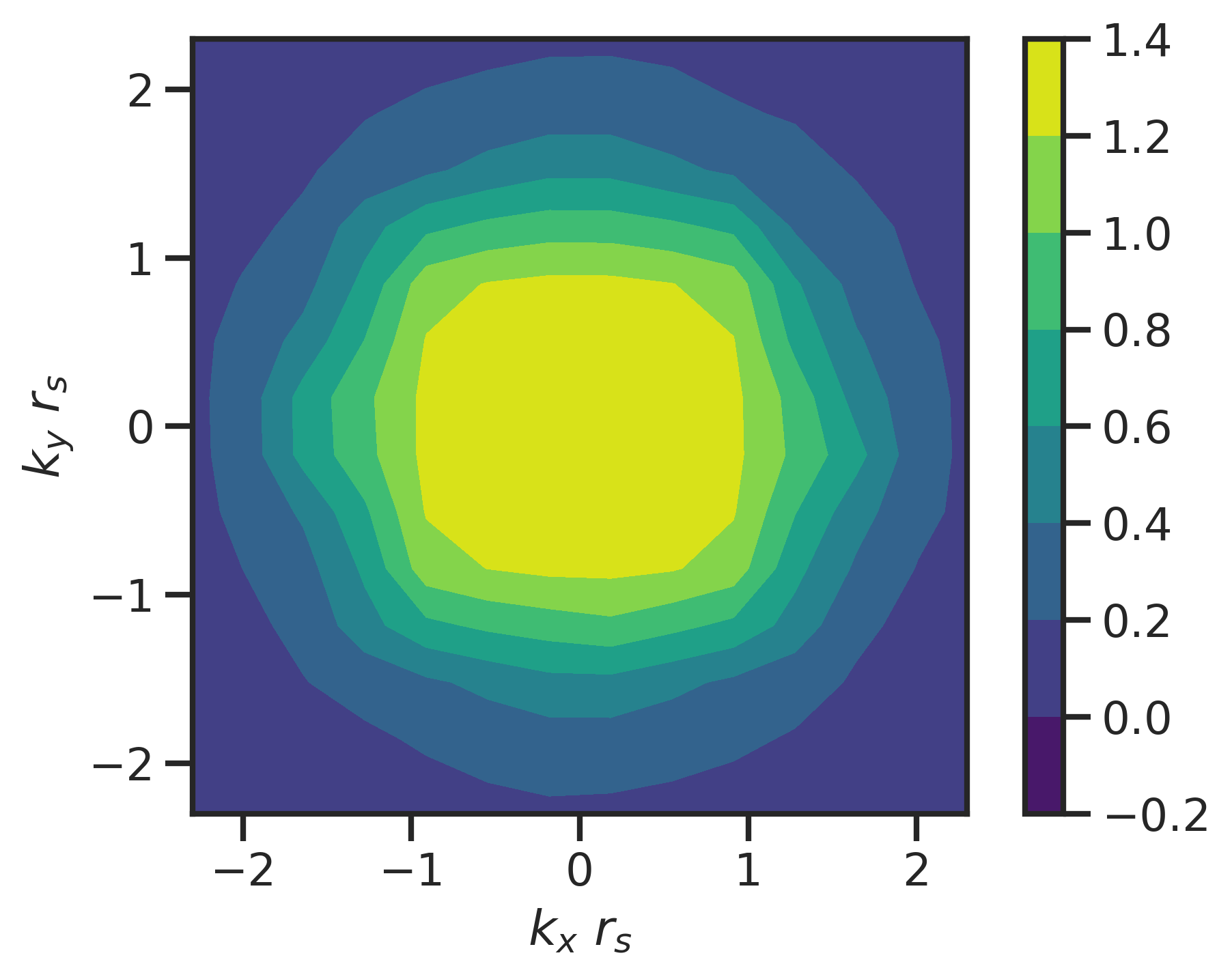
(c) $r_{s}=10$

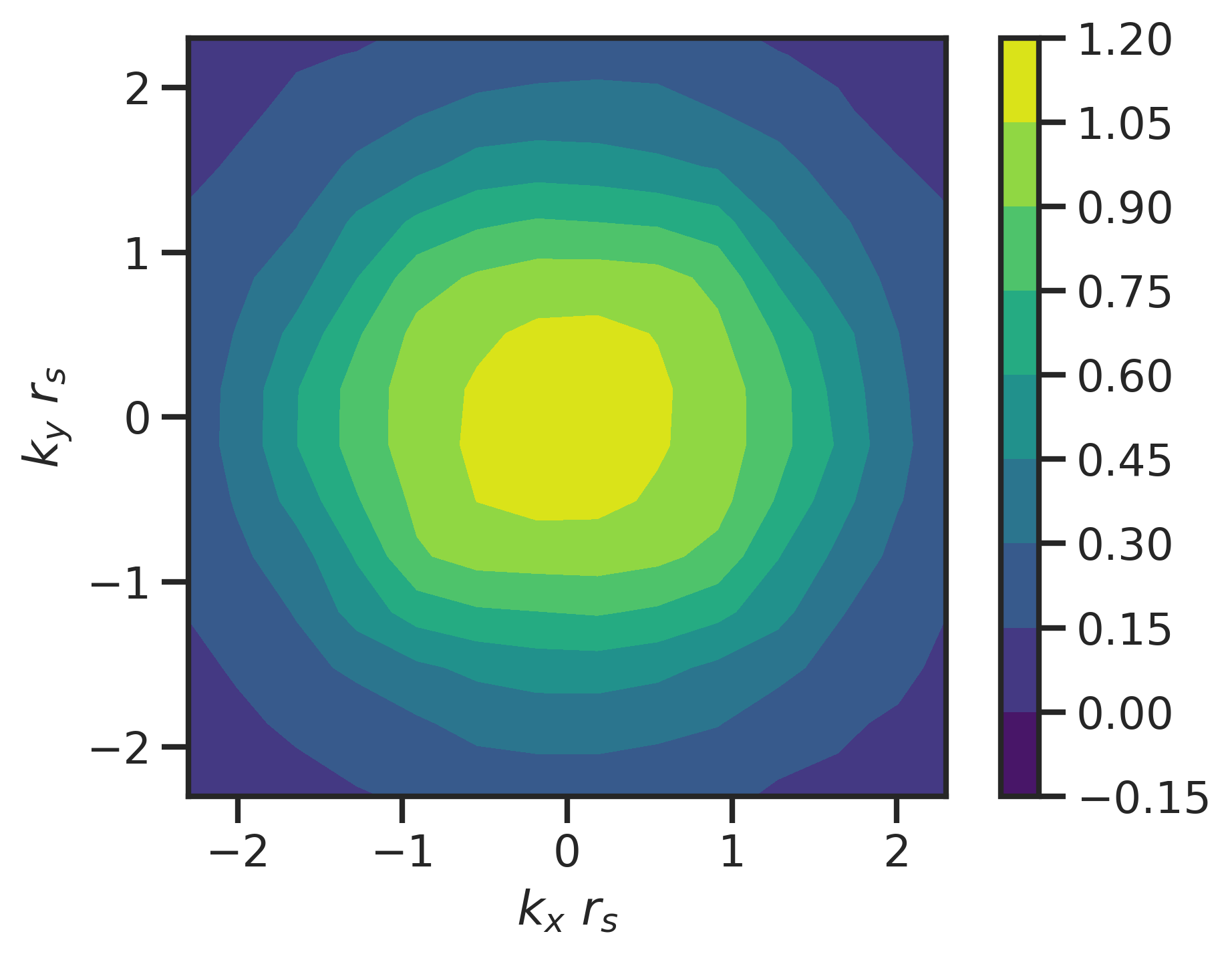
(d) $r_{s}=20$

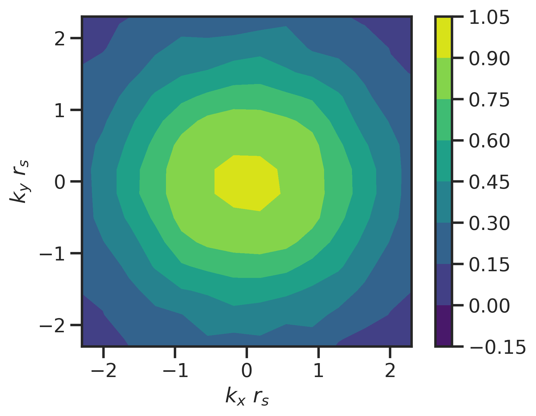
(e) $r_{s}=30$

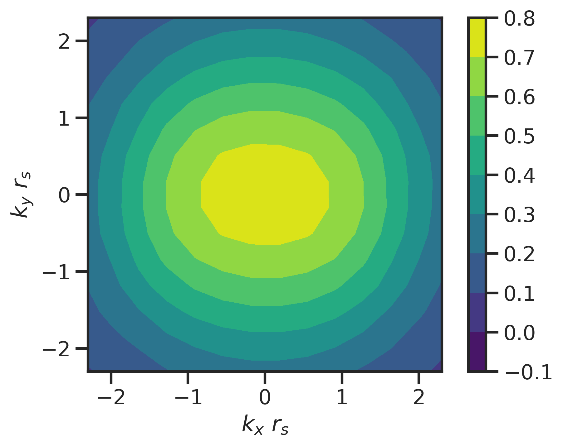
(f) $r_{s}=40$

Figure S5: The momentum distribution $n(\boldsymbol{k})$ and its radial average. The Fermi surface is marked with a dashed black vertical line in (a).

I.4 Anisotropy Observed in Square Simulation Cells

In the main text, the rectangular simulation cell with $N=56$ electrons is constructed to be commensurate with a triangular lattice, which could potentially induce an anisotropy in $g_{s}(r)$ and the one-body density patterns. To ensure the observed anisotropy is not an artifact of this cell choice, we also optimize the (MP)²NQS ansatz in a square cell with $N=58$ electrons. A Wigner crystal is frustrated in a square cell, but similar anisotropy in $g_{s}(r)$ and the one-body density patterns as we approach $r_{s}$ of 35 can be seen in Fig. S6.

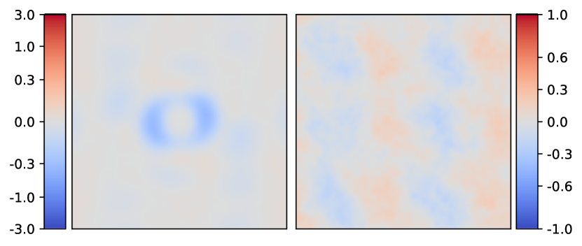
(a) $r_{s}=20$

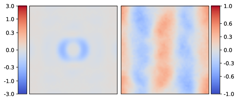
(b) $r_{s}=25$

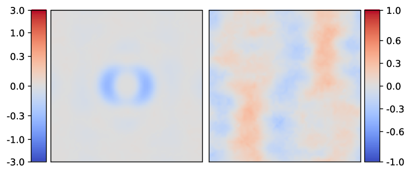
(c) $r_{s}=30$

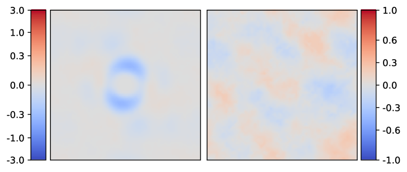
(d) $r_{s}=35$

Figure S6: Spin-spin correlation $g_{s}(r)$ (left) and spin density (right) calculated for the lowest energy states at each $r_{s}$ in a square box with 58 electrons.

I.5 Hamiltonian Details

The jellium Hamiltonian for $N$ electrons with mass $m$ in a uniform dielectric environment with constant $\epsilon$ is

$$H=\dfrac{\hbar^{2}}{2m}\sum\limits_{i=1}^{N}\nabla_{i}^{2}+\dfrac{e^{2}}{4\pi\epsilon}V_{E},$$ (11)

where $V_{E}$ denotes the interaction energy:

$$V_{E}=\sum\limits_{i=1}^{N}\sum\limits_{j=i+1}^{N}\sum\limits_{\boldsymbol{L}_{s}}\dfrac{1}{|\boldsymbol{r}_{i}-\boldsymbol{r}_{j}-\boldsymbol{L}_{s}|}+b.g.\equiv\sum\limits_{i=1}^{N}\sum\limits_{j=i+1}^{N}v_{E}(\boldsymbol{r}_{i}-\boldsymbol{r}_{j})+\dfrac{1}{2}Nv_{M},$$ (12)

where $\boldsymbol{L}_{s}$ is the Bravais lattice generated by the simulation cell with periodic boundary condition. A uniform compensating background is added to enforce charge neutrality. The infinite sum over $\boldsymbol{L}_{s}$ defines the Ewald interaction between a pair of point charges $v_{E}(\boldsymbol{r})$ and the Madelung energy

$$v_{M}\equiv\lim_{\boldsymbol{r}\rightarrow\boldsymbol{0}}[v_{E}(\boldsymbol{r})-1/r],$$ (13)

which is the Ewald potential of a single electron. Direct evaluation of the infinite lattice sum over $\boldsymbol{L}_{s}$ is conditionally convergent, so a dual-space summation algorithm is typically used to evaluate the Ewald interaction

$$v_{E}(\boldsymbol{r})=\sum\limits_{\boldsymbol{L}_{s}}v^{sr}(\boldsymbol{r}-\boldsymbol{L}_{s})+\dfrac{1}{\Omega}\sum\limits_{\boldsymbol{G}_{s}\neq\boldsymbol{0}}v^{lr}_{\boldsymbol{G}_{s}}-\dfrac{1}{\Omega}\lim\limits_{\boldsymbol{G}\rightarrow\boldsymbol{0}}v^{sr}_{\boldsymbol{G}},$$ (14)

where the Coulomb interaction is expressed as the sum of short-range $v^{sr}$ and long-range $v^{lr}$ pieces $1/r=v^{sr}(r)+v^{lr}(r)$ with $v^{sr}_{\boldsymbol{G}}$ and $v^{lr}_{\boldsymbol{G}}$ being their Fourier transforms. In two spatial dimensions, we have the following concrete expressions: $v^{lr}_{G}=2\pi/G~{}\text{erfc}(G/(2\alpha))$, $v^{sr}(r)=1/r~{}\text{erfc}(\alpha r)$ and $\lim\limits_{\boldsymbol{G}\rightarrow\boldsymbol{0}}v^{sr}_{\boldsymbol{G}}=2\sqrt{\pi}/\alpha$, where $\alpha$ is a screening length in reciprocal space. $\boldsymbol{G}_{s}$ is the reciprocal lattice of $\boldsymbol{L}_{s}$. More detailed analysis of the Coulomb interaction with periodic boundary conditions can be found in Refs. Drummond et al. (2008); Holzmann et al. (2016).

The Hamiltonian can be simplified using Hartree atomic units. The Bohr radius is determined by the ratio of the constants $a_{B}=\dfrac{e^{2}}{4\pi\epsilon}/\dfrac{\hbar^{2}}{2m}$ with a vacuum value of $\left(\dfrac{e^{2}}{4\pi\hbar^{2}}\right)~{}\dfrac{m_{e}}{\epsilon_{0}}=0.529177210544$ Å. Using $a_{B}$ as length units, eq. (11) becomes

$$H=E_{h}\left(\dfrac{1}{2}\tilde{\nabla}_{i}^{2}+\tilde{V}_{E}\right),$$ (15)

where the Hartree energy $E_{h}=\dfrac{\hbar^{2}}{ma_{B}^{2}}$ with a vacuum value of $27.21138624598$ eV.

I.6 Wave Function Architectural Details

Our neural network backflow ${\mathcal{N}}$ is based on the message passing network proposed in Pescia et al. (2023). The main idea is to iteratively update two streams of one- and two-body information $\boldsymbol{h}^{(t)}_{i}\in\mathbb{R}^{d_{1}}$ and $\boldsymbol{h}^{(t)}_{ij}\in\mathbb{R}^{d_{2}}$ for each electron $i$ and pair $i$ and $j$, at each message passing layer $t=1,\dots,T$. In each layer $t$, the two streams are combined with the “visible” features of the system, $\boldsymbol{v}_{i}$ and $\boldsymbol{v}_{ij}$, to update the message, $\boldsymbol{m}^{(t)}_{ij}$, between electron pair $i$ and $j$.

$$\boldsymbol{g}^{(t)}_{i}= ~{}\Big{[}\boldsymbol{v}_{i},\ \boldsymbol{h}^{(t-1)}_{i}\Big{]}\,,$$ (16)

$$\boldsymbol{g}^{(t)}_{ij}= ~{}\Big{[}\boldsymbol{v}_{ij},\ \boldsymbol{h}^{(t-1)}_{ij}\Big{]}\,,$$ (17)

$$\boldsymbol{h}^{(t)}_{i}= ~{}{\mathcal{F}}_{1}^{(t)}\Big{(}\sum_{j\neq i}\boldsymbol{m}^{(t)}_{ij},\ \boldsymbol{g}^{(t)}_{i}\Big{)}+\boldsymbol{h}^{(t-1)}_{i}\,,$$ (18)

$$\boldsymbol{h}^{(t)}_{ij}= ~{}{\mathcal{F}}_{2}^{(t)}\Big{(}\boldsymbol{m}^{(t)}_{ij},\ \boldsymbol{g}^{(t)}_{ij}\Big{)}+\boldsymbol{h}^{(t-1)}_{ij}\,,$$ (19)

where ${\mathcal{F}}_{h_{1}}^{(t)}$ and ${\mathcal{F}}_{h_{2}}^{(t)}$ are multi-layer perceptrons (MLPs). We include skip connections He et al. (2016) to facilitate optimization. Here, we set $\boldsymbol{h}_{i}^{(0)}=h_{1}$ and $\boldsymbol{h}_{ij}^{(0)}=h_{2}$ for all $i$ and $j$ to ensure permutation equivariance, where $h_{1}$ and $h_{2}$ are optimizable vectors that are independent of $i$ and $j$ and initialized to zero.

In this work we choose the “visible” features as the following:

$$\boldsymbol{v}_{i}= ~{}\varnothing\,,$$ (20)

$$\boldsymbol{v}_{ij}= ~{}\Big{[}\cos(2\pi A^{-1}\boldsymbol{r}_{ij}),\ \sin(2\pi A^{-1}\boldsymbol{r}_{ij}),\ \norm{\sin(\pi A^{-1}\boldsymbol{r}_{ij})},\ s_{ij}\Big{]}\,,$$ (21)

where $A$ is the cell tensor of the simulation box, $\boldsymbol{r}_{ij}=\boldsymbol{r}_{i}-\boldsymbol{r}_{j}$ is the relative displacement between electron pair $i$ and $j$, and $s_{ij}=2\delta_{s_{i},s_{j}}-1$ assigns $+1$ for parallel spins and $-1$ for antiparallel spins. We use the sine and cosine function as they are smooth and consistent with the periodic boundary condition Pescia et al. (2022). Note that we take the one-body features $\boldsymbol{v}_{i}$ to be empty to explicitly conserve the translational and time-reversal (spin-flipping) symmetry in the construction of neural network backflow ${\mathcal{N}}$. Additional information such as $s_{i}$ and (periodic wrapped) $\boldsymbol{r}_{i}$ can be included in $\boldsymbol{v}_{i}$ to break the symmetry if desired.

The message $\boldsymbol{m}^{(t)}_{ij}$ is computed from another MLP ${\mathcal{F}}_{m}^{(t)}$ that takes the two-body features $\boldsymbol{g}_{ij}^{(t)}$ as input, and is reweighted by an attention matrix ${\mathcal{A}}^{(t)}_{ij}$ which itself is a function of $\boldsymbol{g}^{(t)}_{ij}$ from all electron pairs:

$$\boldsymbol{m}^{(t)}_{ij}= ~{}{\mathcal{A}}_{ij}^{(t)}\Bigl{(}\Bqty{\boldsymbol{g}_{ij}^{(t)}}\Bigr{)}\odot{\mathcal{F}}_{m}^{(t)}\Big{(}\boldsymbol{g}_{ij}^{(t)}\Big{)}\,,$$ (22)

where $\odot$ denotes element-wise multiplication. The attention matrix ${\mathcal{A}}_{ij}^{(t)}$ is computed with the particle attention mechanism proposed in Pescia et al. (2023) with modified scaling and an extra linear layer to facilitate training:

$${\mathcal{A}}_{ij}^{(t)}= ~{}\mathrm{Linear}^{(t)}\circ\mathrm{GELU}\pqty{\frac{1}{\sqrt{N}}\sum_{l}^{N}\boldsymbol{q}_{il}^{(t)}\boldsymbol{k}_{lj}^{(t)}}\,,$$ (23)

$$\boldsymbol{q}_{ij}^{(t)}= ~{}W_{q}^{(t)}\cdot\boldsymbol{g}_{ij}^{(t)}\,,$$ (24)

$$\boldsymbol{k}_{ij}^{(t)}= ~{}W_{k}^{(t)}\cdot\boldsymbol{g}_{ij}^{(t)}\,,$$ (25)

where $W_{q}^{(t)},W_{k}^{(t)}\in\mathbb{R}^{d_{2}\times d_{2}}$ are optimizable weight matrices that act on the feature dimension, and the attention mixes the information on the dimension of electron pairs. The “$\circ$” symbol represents function composition (i.e., $(f\circ g)(x)=f(g(x))$).

All the MLPs denoted by ${\mathcal{F}}$ (${\mathcal{F}}_{1}^{(t)}$, ${\mathcal{F}}_{2}^{(t)}$ and ${\mathcal{F}}_{m}^{(t)}$) contain a single hidden layer with GELU Hendrycks and Gimpel (2016) activation function, i.e.,

$${\mathcal{F}}=\mathrm{Linear}_{2}\circ\mathrm{GELU}\circ\mathrm{Linear}_{1}\,.$$ (26)

In addition, although not written explicitly in the equations, we apply layer normalization Ba et al. (2016) to the inputs of all MLPs and attention layers (${\mathcal{F}}$ and ${\mathcal{A}}_{ij}$) to stabilize optimization.

After the message passing iterations, the backflow displacement ${\mathcal{N}}$ is computed by a linear transform from the final one-body stream $\boldsymbol{h}_{i}^{(T)}$:

$$\boldsymbol{x}_{i}=\boldsymbol{r}_{i}+{\mathcal{N}}(\{\boldsymbol{r}_{i}\})=\boldsymbol{r}_{i}+W_{\mathrm{bf}}\cdot\boldsymbol{h}_{i}^{(T)}\,.$$ (27)

where $W_{\mathrm{bf}}\in\mathbb{R}^{d_{1}\times 2}$ is another weight matrix that maps the one-body stream to the displacement of electron $i$ in two dimensional space.

Similarly, the extra term ${\mathcal{U}}(\{\boldsymbol{r}_{i}\})$ in the Jastrow factor is a sum of one-body contributions, which are computed from the final one-body stream $\boldsymbol{h}_{i}^{(T)}$ and the backflow wrapped coordinates $\boldsymbol{x}_{i}$:

$${\mathcal{U}}(\{\boldsymbol{r}_{i}\})= ~{}\sum_{i}{\mathcal{J}}\pqty{\boldsymbol{h}_{i}^{(T)},\ \mathrm{GELU}\circ\mathrm{Linear_{pre}}(\boldsymbol{x}_{i})}\,,$$ (28)

$${\mathcal{J}}= ~{}\mathrm{Linear}_{L}\circ\mathrm{GELU}\circ\cdots\circ\mathrm{Linear}_{1}\,,$$ (29)

where $\mathrm{Linear_{pre}}:\ \mathbb{R}^{2}\rightarrow\mathbb{R}^{d_{1}}$ is a linear layer that maps the wrapped coordinates $\boldsymbol{x}_{i}$ to a vector of the same dimension as one-body stream $\boldsymbol{h}_{i}$, so that they have comparable contribution in the MLP. ${\mathcal{J}}$ is a MLP with $L-1$ hidden layers that outputs a scalar. In practice, we use $L=4$ for ${\mathcal{J}}$ (i.e., 3 hidden layers). We also apply skip connections between all the hidden layers of ${\mathcal{J}}$ to facilitate optimization.

In our calculations, we set the size of the hidden layers to 32 for all MLPs. We also set $d_{1}=32$ and $d_{2}=26$ so that the size of $\boldsymbol{g}_{i}$ and $\boldsymbol{g}_{ij}$ are equal to 32 as well. In addition, we choose the number of planewaves $N_{k}=3N$ where $N$ is the number of electrons ($2N$ for 120 electron systems) rounding to the nearest closed shell value. This results in a total number of parameters slightly less than 50,000 for calculations with 56 electrons, which can be easily handled by our implementation of stochastic reconfiguration (SR).

To summarize, our wavefunction ansatz largely follows the message passing network from Pescia et al. (2023), with the following major differences:

• We use a linear combination of planewaves for each single-particle orbital $\phi_{a}$, instead of a single planewave or Gaussian function, to allow for automatic detection of liquid and crystal phases.

• We employ a dedicated Jastrow factor term ${\mathcal{U}}$ that depends on both the one-body stream and the backflow coordinates, for better expressivity. We also include the standard pairwise term $u_{2}$ to help capture the cusp condition.

• We apply skip connection and layer normalization as well as some smaller modifications to facilitate optimization.

I.7 Sampling and Optimization Details

We employ the Metropolis-adjusted Langevin algorithm (MALA) Besag (1994) to sample electron configurations from the unnormalized probability given by the trial wavefunction $\absolutevalue{\Psi_{T}}^{2}$. Namely, at each step in the Markov chain, the new electron configuration $\tilde{R}$ is proposed by the following formula:

$$\tilde{R}=R+\tau\gradient\log\absolutevalue{\Psi_{T}(R)}^{2}+\sqrt{2\tau}\xi,$$ (30)

where $R$ is the current electron configuration and $\xi$ is a random variable drawn from the standard Gaussian distribution in $2N$ dimension. The proposed sample is then accepted or rejected according to the Metropolis-Hastings algorithm. The step size $\tau$ is tuned adaptively during the optimization procedure to achieve a suitable acceptance rate.

In practice, we run 1024 Markov chains in parallel, so that we have a batch size of 1024 in the estimation of energy and gradients. To reduce auto-correlation, we run 20 MALA steps between each optimization step, and only use the electron configurations generated from the last step in the optimization. We increase or decrease the step size $\tau$ by 10% every 10 optimization steps, to maintain the harmonic average of acceptance rate staying around $0.65$. We also clip the individual components of the gradient to have a absolute value smaller than one, to stabilize the acceptance rate in the sampling process. In both liquid and crystal phases, the initial electron configurations are chosen to be close to the positions of Wigner crystals with a small Gaussian perturbation. We thermalize the samples with 2000 MALA steps before the optimization starts. We find it is hard to change the spin pattern in the crystal phase in sampling, since it is a rare event for two localized electrons to exchange their position. Therefore we employ two strategy in initializing the spin configurations: aligning with the antiferromagnetic (AFM) pattern in the Wigner crystal or fully random. We find no difference for the two in liquid phase. In crystal phase, the AFM initialization generally achieves lower energy while the random initialization often gets stuck in local minima.

The optimization is conducted with a modified version of stochastic reconfiguration (SR) algorithm named SPRING Goldshlager et al. (2024), which introduced an extra term, analogous to the momentum in stochastic gradient descent, to speed up convergence. Briefly speaking, the update of the parameters at step $t$ is given by

$$d\theta_{t}= ~{}(S+\lambda I)^{-1}(g+\lambda\,\mu\,d\theta_{t-1})\,,$$

$$\theta_{t+1}= ~{}\theta_{t}-\eta\,d\theta_{t}$$ (31)

where $\theta_{t}$ stands for the parameters at step $t$. $S$ and $g$ are the quantum geometric (Fisher) matrix and gradients as in standard SR or natural gradient descent (NGD). $\eta$ is the learning rate, which is set to decay as a inverse function of $t$, $\eta=\eta_{0}(1+(t/T))^{-1}$ with $T$ being the “delay” of the decay. $\lambda$ and $\mu$ are hyperparameters controlling the strength of damping and momentum decay. Setting $\lambda=\mu=0$ will reduce the algorithm to standard SR without diagonal shift. Following the technique in KFAC Martens and Grosse (2015), we also scale $d\theta_{t}$ with a scalar so that its norm induced by the inverse Fisher matrix is smaller than a constant $C$. To efficiently solve the matrix inversion, we take advantage of the sparsity of Fisher matrix $S$ when the number of samples is smaller than the number of parameters, and apply the the Sherman-Morrison-Woodbury formula as described in Ref Ren and Goldfarb (2019).

In practice, we set $\lambda=0.001$, $\mu=0.9$, $T=1000$ and $C=\eta_{0}$. The starting learning rate is chosen dependent on density to accommodate different energy scales, as $\eta_{0}=\{0.5,2,5\}$ for $r_{s}=\{5,10,15\}$, $\eta_{0}=10$ for $15<r_{s}\leq 30$, and $\eta_{0}=15$ for $r_{s}>30$ except that $\eta_{0}=\{20,25,30\}$ for $r_{s}=\{35,36,50\}$.

I.8 Visualizing the Optimized Wave Function

To better understand the final trained wave function ansatz, we can attempt to visualize certain components independently. Through these components, there are signs of the liquid to crystal transition. However, as we are not sampling the wave function distribution, and are ignoring the determinant and Jastrow factor, these signals may be potentially spurious.

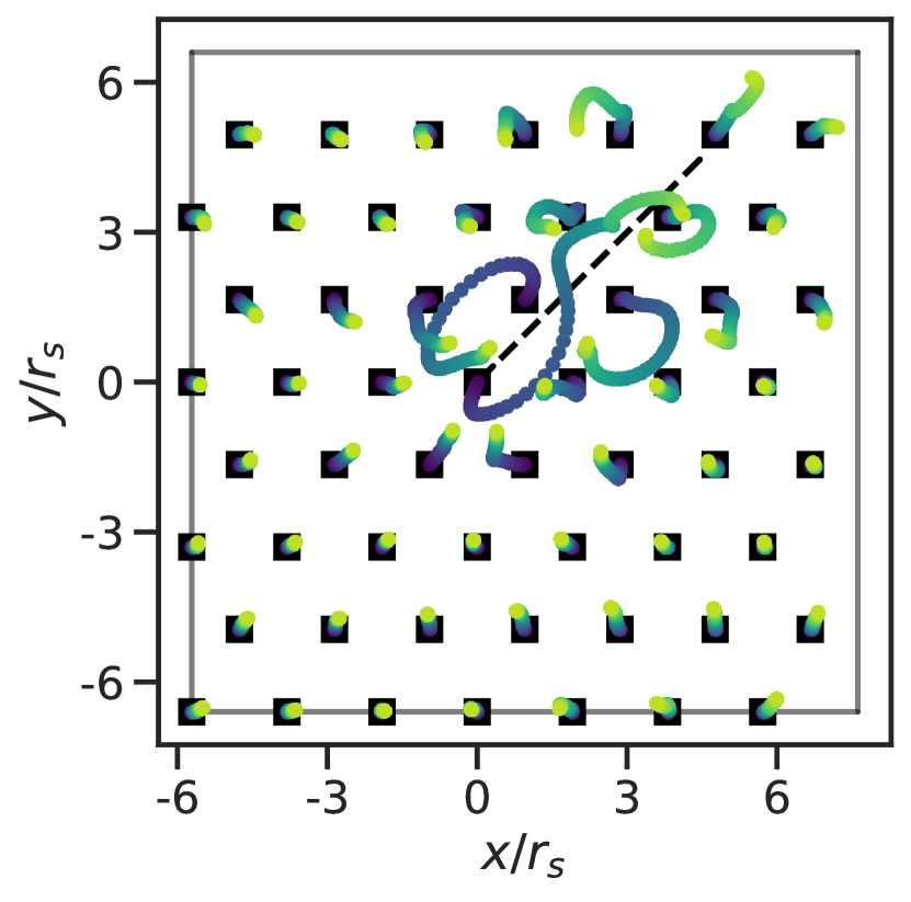
(a) $r_{s}=10$

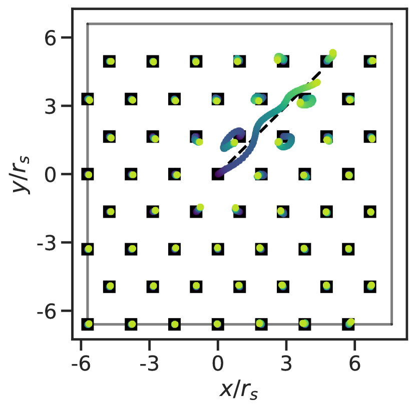
(b) $r_{s}=34$

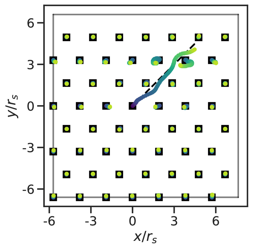
(c) $r_{s}=45$

Figure S7: Final quasiparticle locations of the optimized backflow functions. The center electron is moved to a point along the black dashed line and quasi-particle positions are colored to correspond to electron initial displacement distance (lighter is further distance away). Initial WC positions are shown as black squares.

First we observe the effects of the backflow $\mathcal{N}$ by following the effects of displacing a single electron along a path, shown in Fig. S7. For small $r_{s}$, such as shown in (a), there are strong corrections to the initial positions. For larger $r_{s}$, shown in (b) and (c) there is a much weaker effect and the electrons mostly remain at their initial positions, except when the displaced electron nears another electron. This matches the expected behavior seen in DMC, where backflow is essential to obtaining good liquid results at small to intermediate $r_{s}$.

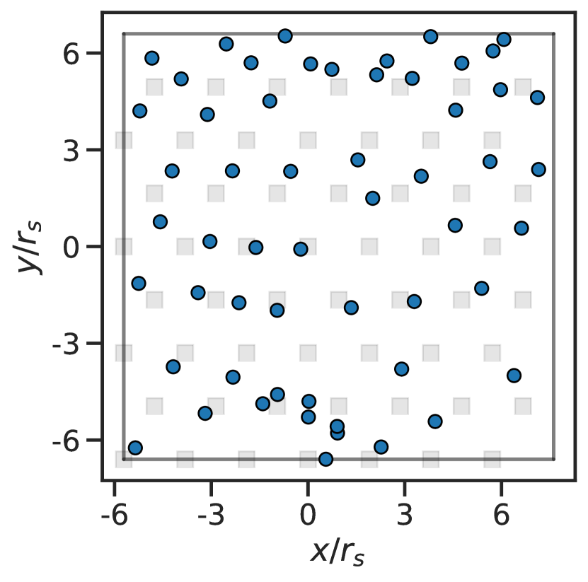
(a) $r_{s}=10$

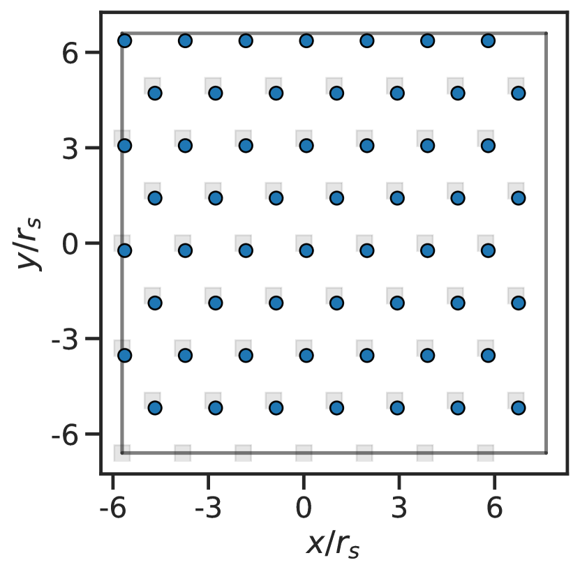
(b) $r_{s}=34$

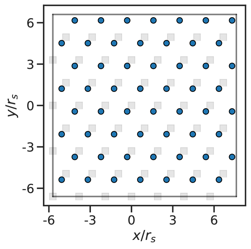
(c) $r_{s}=45$

Figure S8: Final quasiparticle locations $\{r^{out}_{j}\}$ after iterive application of the optimized backflow function. The center electron is displaced a small amount diagonally and the resulting positions are recursively input 10 times with only the final positions plotted. Initial WC positions are shown as black squares.

As another demonstration of backflow correlations, instead of displacing a single electron a varied distance, is to displace the electron once a small amount $\Delta r$ and recursively call the backflow on the output positions

$$\{r^{out}_{j}\}=\mathcal{N}\circ\mathcal{N}\circ\dots\circ\mathcal{N}\left(\{x^{c}_{j}\cdot(1+\Delta r\delta(r-r_{0})\})\right),$$ (32)

where $\{x^{c}_{j}\}$ have the electrons equi-spaced in a WC and $r_{0}$ denotes the electron at the origin. After each application of $\mathcal{N}$, the positions are always projected back into the unit cell. Shown in Fig. S8 are the final quasiparticle positions after a displacement of $|\Delta r/r_{s}|\approx 0.06$ and iteratively applying backflow $\mathcal{N}$ to the resulting output 10 times. We see for small $r_{s}$ (Fig. S8(a)), there is no apparent order to final positions. However for intermediate and large $r_{s}$ (Fig. S8(b)-(c)), the output resembles the initial crystal positions having ‘corrected’ the defect. Note that the shift from the initial positions can be removed by removing the center of mass movement.

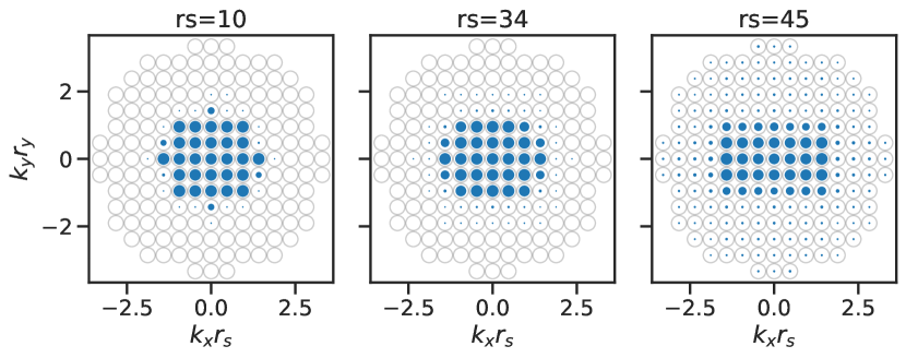
(a) Spin Averaged Norm $|c_{k}|$

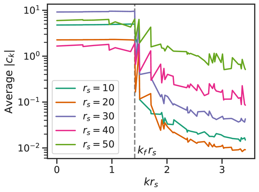
(b) Spin and Radially Averaged Norm

Figure S9: Analysis of the optimized multiple planewave $c_{ak}^{\sigma}$ values.

Then we can observe how the multi planewave coefficients $c_{ak}^{\sigma}$ are optimized across the different values of $r_{s}$, shown in Fig. S9. First, the norm is taken over the electron index $a$ then averaged over spins ($\sigma=\{\uparrow\downarrow\}$) such that $|c_{k}|=1/2\sum_{\sigma}(\sum_{a}|c_{ak}^{\sigma}|^{2})^{1/2}$. In Fig. S9(a), each included $k$ value, a total of $N_{k}=3N$, is plotted as an open circle, while the magnitude of $|c_{k}|$ is shown as the relative to the maximum value. For low to intermediate $r_{s}$, only those $k$ points around $k_{F}$ are relatively strong although points further from $k_{F}$ pick up weight as $r_{s}$ increases. If we consider a threshold of $|c_{k}|\geq O(10^{-1})$ as significant, in the liquid phase, less than $40\%$ of the $k$ points reach that threshold but in the crystal phase nearly all of them do. This can be seen in Fig. S9(b), where by radially averaging $|c_{k}|$, as $r_{s}$ increases the tail of the magnitudes at large $|k|$ slowly increases, until all $|c_{k}|$ are roughly on the same order.

References

- Ceperley and Alder (1980) D. M. Ceperley and B. J. Alder, “Ground State of the Electron Gas by a Stochastic Method,” Physical Review Letters 45, 566–569 (1980).
- Tanatar and Ceperley (1989) B. Tanatar and D. M. Ceperley, “Ground state of the two-dimensional electron gas,” Physical Review B 39, 5005–5016 (1989).
- Attaccalite et al. (2002) Claudio Attaccalite, Saverio Moroni, Paola Gori-Giorgi, and Giovanni B. Bachelet, “Correlation Energy and Spin Polarization in the 2D Electron Gas,” Physical Review Letters 88, 256601 (2002).
- Drummond and Needs (2009) N. D. Drummond and R. J. Needs, “Phase Diagram of the Low-Density Two-Dimensional Homogeneous Electron Gas,” Physical Review Letters 102, 126402 (2009).
- Hossain et al. (2020) M. S. Hossain, M. K. Ma, K. A. Villegas Rosales, Y. J. Chung, L. N. Pfeiffer, K. W. West, K. W. Baldwin, and M. Shayegan, “Observation of spontaneous ferromagnetism in a two-dimensional electron system,” Proceedings of the National Academy of Sciences 117, 32244–32250 (2020).
- Hossain et al. (2021) Md. S. Hossain, M. K. Ma, K. A. Villegas-Rosales, Y. J. Chung, L. N. Pfeiffer, K. W. West, K. W. Baldwin, and M. Shayegan, “Spontaneous Valley Polarization of Itinerant Electrons,” Physical Review Letters 127, 116601 (2021).
- Hossain et al. (2022) Md. S. Hossain, M. K. Ma, K. A. Villegas-Rosales, Y. J. Chung, L. N. Pfeiffer, K. W. West, K. W. Baldwin, and M. Shayegan, “Anisotropic Two-Dimensional Disordered Wigner Solid,” Physical Review Letters 129, 036601 (2022).
- Smoleński et al. (2021) Tomasz Smoleński, Pavel E. Dolgirev, Clemens Kuhlenkamp, Alexander Popert, Yuya Shimazaki, Patrick Back, Xiaobo Lu, Martin Kroner, Kenji Watanabe, Takashi Taniguchi, Ilya Esterlis, Eugene Demler, and Ataç Imamoğlu, “Signatures of Wigner crystal of electrons in a monolayer semiconductor,” Nature 595, 53–57 (2021).
- Falson et al. (2022) J. Falson, I. Sodemann, B. Skinner, D. Tabrea, Y. Kozuka, A. Tsukazaki, M. Kawasaki, K. Von Klitzing, and J. H. Smet, “Competing correlated states around the zero-field Wigner crystallization transition of electrons in two dimensions,” Nature Materials 21, 311–316 (2022).
- Falakshahi and Waintal (2005) Houman Falakshahi and Xavier Waintal, “Hybrid Phase at the Quantum Melting of the Wigner Crystal,” Physical Review Letters 94, 046801 (2005).
- Spivak and Kivelson (2004) Boris Spivak and Steven A. Kivelson, “Phases intermediate between a two-dimensional electron liquid and wigner crystal,” Physical Review B 70 (2004), 10.1103/physrevb.70.155114.
- Kim et al. (2023) Kyung-Su Kim, Ilya Esterlis, Chaitanya Murthy, and Steven A. Kivelson, “Dynamical defects in a two-dimensional Wigner crystal: self-doping and kinetic magnetism,” arXiv e-prints , arXiv:2309.13121 (2023), arXiv:2309.13121 [cond-mat.str-el] .
- Li et al. (2021) Hongyuan Li, Shaowei Li, Emma C. Regan, Danqing Wang, Wenyu Zhao, Salman Kahn, Kentaro Yumigeta, Mark Blei, Takashi Taniguchi, Kenji Watanabe, Sefaattin Tongay, Alex Zettl, Michael F. Crommie, and Feng Wang, “Imaging two-dimensional generalized Wigner crystals,” Nature 597, 650–654 (2021).
- Shabani et al. (2021) Sara Shabani, Dorri Halbertal, Wenjing Wu, Mingxing Chen, Song Liu, James Hone, Wang Yao, D. N. Basov, Xiaoyang Zhu, and Abhay N. Pasupathy, “Deep moiré potentials in twisted transition metal dichalcogenide bilayers,” Nature Physics 17, 720–725 (2021).
- Regan et al. (2020) Emma C. Regan, Danqing Wang, Chenhao Jin, M. Iqbal Bakti Utama, Beini Gao, Xin Wei, Sihan Zhao, Wenyu Zhao, Zuocheng Zhang, Kentaro Yumigeta, Mark Blei, Johan D. Carlström, Kenji Watanabe, Takashi Taniguchi, Sefaattin Tongay, Michael Crommie, Alex Zettl, and Feng Wang, “Mott and generalized Wigner crystal states in WSe2/WS2 moiré superlattices,” Nature 579, 359–363 (2020).
- Sung et al. (2023) Jiho Sung, Jue Wang, Ilya Esterlis, Pavel A. Volkov, Giovanni Scuri, You Zhou, Elise Brutschea, Takashi Taniguchi, Kenji Watanabe, Yubo Yang, Miguel A. Morales, Shiwei Zhang, Andrew J. Millis, Mikhail D. Lukin, Philip Kim, Eugene Demler, and Hongkun Park, “Observation of an electronic microemulsion phase emerging from a quantum crystal-to-liquid transition,” arXiv e-prints , arXiv:2311.18069 (2023), arXiv:2311.18069 [cond-mat.str-el] .
- Carleo and Troyer (2017) Giuseppe Carleo and Matthias Troyer, “Solving the quantum many-body problem with artificial neural networks,” Science 355, 602–606 (2017).
- Pfau et al. (2020) David Pfau, James S. Spencer, Alexander G. D. G. Matthews, and W. M. C. Foulkes, “Ab Initio solution of the many-electron Schrödinger equation with deep neural networks,” Physical Review Research 2, 033429 (2020).
- Hermann et al. (2020) Jan Hermann, Zeno Schätzle, and Frank Noé, “Deep-neural-network solution of the electronic schrödinger equation,” Nature Chemistry 12, 891–897 (2020).
- Hermann et al. (2023) Jan Hermann, James Spencer, Kenny Choo, Antonio Mezzacapo, W. M. C. Foulkes, David Pfau, Giuseppe Carleo, and Frank Noé, “Ab initio quantum chemistry with neural-network wavefunctions,” Nature Reviews Chemistry 7, 692–709 (2023).
- Pescia et al. (2022) Gabriel Pescia, Jiequn Han, Alessandro Lovato, Jianfeng Lu, and Giuseppe Carleo, “Neural-network quantum states for periodic systems in continuous space,” Physical Review Research 4, 023138 (2022).
- Pescia et al. (2023) Gabriel Pescia, Jannes Nys, Jane Kim, Alessandro Lovato, and Giuseppe Carleo, “Message-passing neural quantum states for the homogeneous electron gas,” arXiv preprint arXiv:2305.07240 (2023).
- Ceperley et al. (1977) David Ceperley, Geoffrey V Chester, and Malvin H Kalos, “Monte carlo simulation of a many-fermion study,” Physical Review B 16, 3081 (1977).
- Feynman (1954) R. P. Feynman, “Atomic Theory of the Two-Fluid Model of Liquid Helium,” Physical Review 94, 262–277 (1954).
- Feynman and Cohen (1956) R. P. Feynman and Michael Cohen, “Energy Spectrum of the Excitations in Liquid Helium,” Physical Review 102, 1189–1204 (1956).
- Kwon et al. (1993) Yongkyung Kwon, D. M. Ceperley, and Richard M. Martin, “Effects of three-body and backflow correlations in the two-dimensional electron gas,” Physical Review B 48, 12037–12046 (1993).
- Holzmann et al. (2003) M. Holzmann, D. M. Ceperley, C. Pierleoni, and K. Esler, “Backflow correlations for the electron gas and metallic hydrogen,” Physical Review E 68, 046707 (2003).
- Taddei et al. (2015) Michele Taddei, Michele Ruggeri, Saverio Moroni, and Markus Holzmann, “Iterative backflow renormalization procedure for many-body ground-state wave functions of strongly interacting normal Fermi liquids,” Physical Review B 91, 115106 (2015).
- Ruggeri et al. (2018) Michele Ruggeri, Saverio Moroni, and Markus Holzmann, “Nonlinear Network Description for Many-Body Quantum Systems in Continuous Space,” Physical Review Letters 120, 205302 (2018).
- Cassella et al. (2023) Gino Cassella, Halvard Sutterud, Sam Azadi, N. D. Drummond, David Pfau, James S. Spencer, and W. M. C. Foulkes, “Discovering Quantum Phase Transitions with Fermionic Neural Networks,” Physical Review Letters 130, 036401 (2023).
- Wilson et al. (2023) Max Wilson, Saverio Moroni, Markus Holzmann, Nicholas Gao, Filip Wudarski, Tejs Vegge, and Arghya Bhowmik, “Neural network ansatz for periodic wave functions and the homogeneous electron gas,” Physical Review B 107, 235139 (2023).
- Besag (1994) Julian Besag, “Comments on “representations of knowledge in complex systems” by u. grenander and mi miller,” J. Roy. Statist. Soc. Ser. B 56, 4 (1994).
- Sorella (1998) Sandro Sorella, “Green function monte carlo with stochastic reconfiguration,” Physical review letters 80, 4558 (1998).
- Sorella (2005) Sandro Sorella, “Wave function optimization in the variational monte carlo method,” Physical Review B 71, 241103 (2005).
- Goldshlager et al. (2024) Gil Goldshlager, Nilin Abrahamsen, and Lin Lin, “A kaczmarz-inspired approach to accelerate the optimization of neural network wavefunctions,” arXiv preprint arXiv:2401.10190 (2024).
- (36) DMC calculations performed using QMCPACK 3.15.9 Kim et al. (2018); Kent et al. (2020) with appropriate 2D modifications.
- Bishop and Lührmann (1982) RF Bishop and KH Lührmann, “Electron correlations. ii. ground-state results at low and metallic densities,” Physical Review B 26, 5523 (1982).
- Lewin et al. (2019) Mathieu Lewin, Elliott H Lieb, and Robert Seiringer, “Floating wigner crystal with no boundary charge fluctuations,” Physical Review B 100, 035127 (2019).
- Azadi et al. (2024) Sam Azadi, N. D. Drummond, and S. M. Vinko, “Quantum Monte Carlo study of the phase diagram of the two-dimensional uniform electron liquid,” arXiv e-prints , arXiv:2405.00425 (2024), arXiv:2405.00425 [cond-mat.str-el] .
- Kim et al. (2018) Jeongnim Kim, Andrew D Baczewski, Todd D. Beaudet, Anouar Benali, M. Chandler Bennett, Mark A. Berrill, Nick S. Blunt, Edgar Josué Landinez Borda, Michele Casula, David M. Ceperley, Simone Chiesa, Bryan K. Clark, Raymond C. Clay, Kris T. Delaney, Mark Dewing, Kenneth P. Esler, Hongxia Hao, Olle Heinonen, Paul R C Kent, Jaron T. Krogel, Ilkka Kylänpää, Ying Wai Li, M. Graham Lopez, Ye Luo, Fionn D. Malone, Richard M. Martin, Amrita Mathuriya, Jeremy McMinis, Cody A. Melton, Lubos Mitas, Miguel A. Morales, Eric Neuscamman, William D. Parker, Sergio D. Pineda Flores, Nichols A. Romero, Brenda M. Rubenstein, Jacqueline A R Shea, Hyeondeok Shin, Luke Shulenburger, Andreas F. Tillack, Joshua P. Townsend, Norm M. Tubman, Brett Van Der Goetz, Jordan E. Vincent, D ChangMo Yang, Yubo Yang, Shuai Zhang, and Luning Zhao, “QMCPACK : an open source ab initio quantum Monte Carlo package for the electronic structure of atoms, molecules and solids,” Journal of Physics: Condensed Matter 30, 195901 (2018), 1802.06922 .
- Kent et al. (2020) P. R. C. Kent, Abdulgani Annaberdiyev, Anouar Benali, M. Chandler Bennett, Edgar Josué Landinez Borda, Peter Doak, Hongxia Hao, Kenneth D. Jordan, Jaron T. Krogel, Ilkka Kylänpää, Joonho Lee, Ye Luo, Fionn D. Malone, Cody A. Melton, Lubos Mitas, Miguel A. Morales, Eric Neuscamman, Fernando A. Reboredo, Brenda Rubenstein, Kayahan Saritas, Shiv Upadhyay, Guangming Wang, Shuai Zhang, and Luning Zhao, “QMCPACK: Advances in the development, efficiency, and application of auxiliary field and real-space variational and diffusion quantum Monte Carlo,” The Journal of Chemical Physics 152, 174105 (2020), 2003.01831 .
- Drummond et al. (2008) N. D. Drummond, R. J. Needs, A. Sorouri, and W. M. C. Foulkes, “Finite-size errors in continuum quantum Monte Carlo calculations,” Physical Review B 78, 125106 (2008).
- Holzmann et al. (2016) Markus Holzmann, Raymond C. Clay, Miguel A. Morales, Norm M. Tubman, David M. Ceperley, and Carlo Pierleoni, “Theory of finite size effects for electronic quantum monte carlo calculations of liquids and solids,” Phys. Rev. B 94, 035126 (2016).
- He et al. (2016) Kaiming He, Xiangyu Zhang, Shaoqing Ren, and Jian Sun, “Deep residual learning for image recognition,” in Proceedings of the IEEE conference on computer vision and pattern recognition (2016) pp. 770–778.
- Hendrycks and Gimpel (2016) Dan Hendrycks and Kevin Gimpel, “Gaussian error linear units (gelus),” arXiv preprint arXiv:1606.08415 (2016).
- Ba et al. (2016) Jimmy Lei Ba, Jamie Ryan Kiros, and Geoffrey E Hinton, “Layer normalization,” arXiv preprint arXiv:1607.06450 (2016).
- Martens and Grosse (2015) James Martens and Roger Grosse, “Optimizing neural networks with kronecker-factored approximate curvature,” in International conference on machine learning (PMLR, 2015) pp. 2408–2417.
- Ren and Goldfarb (2019) Yi Ren and Donald Goldfarb, “Efficient subsampled gauss-newton and natural gradient methods for training neural networks,” arXiv preprint arXiv:1906.02353 (2019).