Nonperturbative Effects in Energy Correlators:
From Characterizing Confinement Transition to Improving Extraction
Abstract
Energy correlators provide a powerful observable to study fragmentation dynamics in QCD. We demonstrate that the leading nonperturbative corrections for projected -point energy correlators are described by the same universal parameter for any , which has already been determined from other event shape fits. Including renormalon-free nonperturbative corrections substantially improves theoretical predictions of energy correlators, notably the transition into the confining region at small angles. Nonperturbative corrections are shown to have a significant impact on extractions.
Introduction. The angular distribution of energy in high-energy scattering offers a powerful experimental lens through which to explore the Lorentzian dynamics of Quantum Chromodynamics (QCD). Central to this exploration is the energy flow operator [1, 2, 3, 4, 5, 6, 7, 8],
| (1) |
which relates the energy-momentum tensor in QCD to the energy captured by a detector in the direction . Measuring correlators of these operators through -point energy correlators (ENC), enable us to uncover subtle quantum correlations in collider energy distributions [9, 10, 11, 12, 13, 14]. The state could be generated by a local source such as an electromagnetic current injecting invariant mass , or denote a collection of particles such as a jet [15]. As the angles are varied, the associated invariant mass scale reveals numerous intrinsic and emergent scales in QCD [16, 17, 18, 15, 19, 20, 21, 22, 23, 24, 25, 26, 27].
In this Letter, we determine the leading nonperturbative effects for projected ENCs (pENCs)[14], which measure only the largest angle . We find they are determined by two universal hadronic parameters, and , with perturbatively calculable and dependence. The same appear in other observables, providing exciting prospects for testing universality and making parameter-free predictions. Eliminating the renormalon ambiguity in , we find an improved description of the transition from the partonic to confining region for pENCs, see Fig. 1. Motivated by the recent CMS measurement of using a ratio of energy correlators [28], we assess the impact of nonperturbative effects in ratios and the accuracy of estimates based on Monte Carlo generators (MC).
The hadronic final state in collisions provides a pristine environment for examining the nature of QCD fragmentation. By exploring the energy correlations across the entire scattering event — similar to cosmic surveys mapping the sky — we can elegantly map particle interactions at their most fundamental level. The two-point energy correlator (EEC) is given by
| (2) |
where refers to the hadronic final state sourced by the electromagnetic current , is the leptonic tensor, and . The second equality gives us an operator definition of EEC in terms of a correlation function of energy flow operators. Exploiting this operator definition has enhanced the interpretability of experimental data [28, 30, 31, 32], facilitating the application of a wide array of modern field-theoretic techniques, and inspired precision calculations [33, 34, 35, 36, 37, 38, 39, 40, 13, 41, 42, 43, 44, 45, 39, 46, 47, 48, 6, 7, 49, 50, 51, 52].
Examining the effects of hadronization on such correlations has been one of the prime objectives of collider-QCD studies. In a pioneering paper [3], the leading hadronization power corrections for EEC were first identified, described by the matrix element
| (3) |
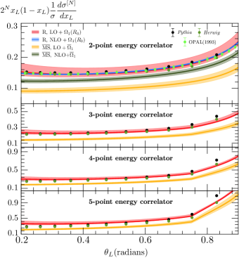
where denotes the color channel [53, 54], and and . The Wilson lines, , are oriented along back-to-back light-like directions , and source the soft hadrons, and is the transverse energy flow operator. Here is the same leading power correction appearing in event shapes in the dijet limit [55, 56, 57, 29, 58]. In Ref. [59], the leading renormalon ambiguity was calculated for the EEC, and results for the EEC were presented eliminating this leading ambiguity, and utilizing a value for the leading power correction obtained from an earlier thrust fit [29]. Away from kinematic endpoints, this reorganization addressed the long-standing discrepancies between perturbative calculations and collider data [60, 61, 62, 63] for EEC without the need to fit any parameters as shown in the top panel of Fig. 2.
The pENCs that we study are defined by
| (4) |
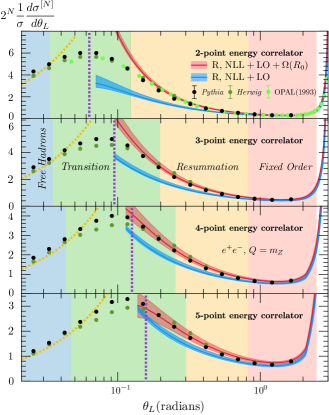
Nonperturbative effects grow in significance as we approach the kinematic endpoints, , where the energy scale becomes nonperturbative, . Here energy correlators exhibit a striking transition from the perturbative partonic scaling region to freely propagating confined hadrons with vanishing correlations. This transition has been observed for and in jets with hadron collider data [28, 31, 32]. For this transition is clearly visible in Fig. 1 for in Pythia and Herwig simulations.
Power corrections and renormalon analysis. Away from for pENCs from , the leading corrections at lowest order in arise when one of the energy flow detectors aligns with the direction of soft hadrons, while the remaining detectors align with one of the energetic dijets. Thus, for this contribution specifies the angle between the soft hadron direction and the energetic dijet, and there are different ways to place a detector on soft hadrons. Using and , we arrive at the form of leading nonperturbative power corrections for pENCs from collisions:
| (5) |
where is the perturbative result and is the nonperturbative power correction in the scheme. The overall in the second term, also present in the first term, arises from the energy weighting needed to ensure the sum rule . For this result was derived in Ref. [3] with nonperturbative matrix element as defined in Eq. (3), and we extend this to . For typical event shapes, an analogous relation for the leading power correction is only valid in the dijet limit. This is because the measurement in such event shapes is not inclusive and directly constrains the momentum of the final state. In contrast, energy correlations for any angular separation are inclusive, such that this relation remains valid across all angles except when . (In the back-to-back limit, contributions from detectors on three particles also give a leading contribution.) At higher orders in the and dependence can be different.
Next, we bring in insights from renormalon analysis of bubble-chain diagrams, where the leading terms at each perturbative order give a mechanism for examining the nature of power corrections in asymptotic perturbative series in [64, 65, 66]. Renormalon analysis has various benefits: It provides an independent check on the coefficient of the nonperturbative matrix element, including the and dependence in Eq. (5). Also removing renormalon ambiguities present in from both and in Eq. (5) improves the convergence of the series already at low orders in perturbation theory. Furthermore, with the renormalon ambiguity removed, the parameters can now fully capture the leading nonperturbative effects. The bubble sum calculation for pENCs is a simple extension of Ref. [59], and we find a ‘’ pole in the Borel space [67, 68, 69] with the ambiguity from the contour around this pole given by
| (6) |
This confirms the and dependence in Eq. (5).
We restore the separation of scales in power corrections by using the R scheme with a subtraction scale [70, 71, 72, 73] to remove the renormalon ambiguities from both and in the scheme. This can be done by defining and as
| (7) | ||||
where the coefficients are those of the original series and are functions of logarithms with coefficients appropriately chosen to remove the renormalon [70, 29, 73, 74, 29]. To ensure that is of the same parametric size as , we generally choose such that the change is , and resum the large logarithms between and using -RGE [71, 29, 73]. Using the and values determined from the thrust fit in Ref. [29], we convert to the R scheme #2 of Ref. [75], and add 23% from hadron mass corrections following [58, 59], yielding . We investigate the (small) dependence on the R scheme choice in a future paper [76].
In Fig. 2, we present fixed-order calculations at at the -pole, , incorporating power corrections for both the and R schemes. Uncertainty bands are from factor of two scale variations around . We compare our results with MC simulations from Pythia and Herwig, and with OPAL data [63] for . For , we observe improved perturbative convergence in the R scheme relative to the scheme and a remarkable agreement with the OPAL data (consistent with Ref. [59] in a different R scheme). For higher-point cases, with a LO analysis, we find that the R scheme leads to better agreement with MC, similar to . Thus we anticipate similar improvements in perturbative convergence for , indicating that the R scheme is effective in removing the dominant renormalon ambiguity. This provides strong motivation for comparing R scheme-improved perturbative predictions with real-world collider data, particularly with upcoming revised LEP data analyses on the horizon [77].
Imaging Hadronization Transition. The leading scaling behavior of pENCs in the small angle limit is captured through an iterative application of the light-ray operator product expansion (OPE) [52, 78, 8, 5, 6, 7, 79] and is given by the twist- spin- anomalous dimension. A QCD factorization theorem for pENC in the collinear limit, which captures both this anomalous scaling and the RG-flow of the coupling, was derived both for colliders [13] and for jets in hadron colliders [15]. In the small angle limit, the cumulant of the pENC , factorizes as
| (8) | ||||
where denotes a hard function that describes the production of the energetic particles, and is the -point energy correlator jet function sensitive to the dependence of the observable ( is known at next-to-next-to-leading logarithmic order for [13, 80]). Both functions are vectors in the gluon/quark space. For hadron colliders, also includes parton distribution functions. The evolution equation for the jet function is
| (9) |
where is the singlet time-like splitting matrix.
As the renormalon ambiguity plagues pENCs at all angles, including the small-angle region, it must also be removed from these jet functions. Demanding consistency with the RG and the prediction in Eq. (5) for nonperturbative corrections in the fixed order region, the power corrections to the jet functions must take the form
| (10) |
where both and are perturbative coefficients. Next we define
| (11) |
as the perturbative series of the jet function, and analogously for . We use tree-level normalization , and explicit results for can be found in Ref. [14]. Due to the presence of the in the term, the logarithmic structure of the power correction contained in has the same evolution as .111This reproduces the observation made by Ref. [81] that the spin of the anomalous dimension of the power suppressed term is decreased by . Therefore, the single logarithm in is taken equal to that of , while the constant term can differ. Computing the leading renormalon for we find a result consistent with Eq. (Nonperturbative Effects in Energy Correlators: From Characterizing Confinement Transition to Improving Extraction). An R scheme jet function which cancels the renormalon can be defined by
| (12) | |||
where are identical to those in Eq. (7).
In Fig. 1, we clearly see the importance of incorporating the nonperturbative corrections. Looking from the right, we first encounter the fixed order region shown in red, which is discussed in Fig. 2. We then hit the perturbative resummation region, shown in orange, where quarks and gluons radiate to give us the scaling predicted by the light-ray OPE. The radiating partons eventually lose enough energy and are confined to form a bound state of hadrons, which manifests itself in the turnover in the green region, now also observed in numerous experimental datasets across many collaborations [28, 30, 31, 32], and through string or clustering fragmentation [82, 83, 84, 85, 86] in MC simulations as illustrated in the figure for Pythia and Herwig. Finally, we reach the free hadron region in blue, where correlations vanish. The golden dashed line is a linear fit to the correlations in the free hadron region, , corresponding to a uniform distribution in .
We see that incorporating nonperturbative power corrections in the R scheme significantly improves our description of the approach to the hadronization peak from the parton scaling region. As we get closer to this peak, the nonperturbative effects no longer remain subleading. Since the first term in Eq. (5) scales as , this occurs when for the -point correlator (up to anomalous scaling). For this predicts a relation between the peak location for relative to . Fixing the constant using the EEC and above, we find for EEC , which then predicts the vertical purple dotted lines in Fig. 1, consistent with the peak locations for higher .
Strong Coupling Determination. By taking the ratio of pENCs to EEC, we eliminate their classical scaling and isolate the anomalous scaling proportional to , making the ratio in the small angle region an ideal observable for cleanly extracting [14]. Due to the monotonicity of twist-2 spin- anomalous dimensions as a function of , the slope of the ratio increases with [87]. This method recently yielded the most precise jet substructure based extraction at the LHC, with the CMS collaboration achieving an accuracy of 4% with by analyzing the ratio of pE3C to EEC for a range of jet [28]. Generally, it was expected that nonperturbative contributions across different values of would cancel out in the ratio [17, 80, 28]. This expectation led CMS to use perturbative theoretical predictions [80], combined with MC modeling of hadronization effects, in the CMS extraction. With our systematic prescription for removing renormalon ambiguities and our prediction for the relation between nonperturbative corrections for different values, we are well-positioned to assess the magnitude of these effects in determination using pENCs with our field theory based approach.
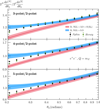
In Fig. 3, we compare the pENC/EEC ratio with and without nonperturbative power corrections at for . Although in the perturbative region shown one fits for using the full functional form, the impact of various parameters can be estimated from changes to the slope in a linear fit approximation, which becomes better further away from the transition region. As the angle approaches the transition region, we observe that the MC simulations begin to deviate from the linear slope, which nonperturbative corrections capture well.
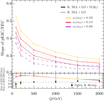
In Fig. 4, we examine the impact of nonperturbative power corrections by plotting the slope of pE3C/EEC within the perturbative scaling region to ensure separation from the transition region. This visualization clearly shows the decreasing slope as we move to higher , serving as a clear signature of asymptotic freedom. Contrary to earlier observations, nonperturbative power corrections significantly impact the ratio. In the lower panel of Fig. 4, we plot the ratio of hadronic and partonic slopes, and see that the size of hadronization correction in our analytic calculation decreases from 20% down to 5% for increasing , and is much larger than the small effects observed in Pythia and Herwig. This underscores the danger of solely relying on the difference between hadronic and partonic MC to model hadronization corrections in perturbative calculations.
Comparing the dashed and solid lines in Fig. 4 shows a degeneracy between including nonperturbative power corrections and increasing values. This illustrates the importance of controlling nonperturbative corrections to achieve a precise fit for . For example, at GeV including nonperturbative corrections is a 10% effect in the direction of decreasing .
Conclusion. We performed a model-independent assessment of nonperturbative corrections on projected -point energy correlators, and derived a relation between these corrections. Our predictions in a renormalon-free scheme improve hadron-level results for both large and small angle regions. This analysis provides a strong motivation for revisiting extraction using our model-independent predictions for nonperturbative corrections. This is particularly pertinent to upcoming precision analyses of LEP data and jet measurements at hadron colliders, including both the LHC and RHIC.
Acknowledgements.
Acknowledgments. We thank Hao Chen, Philip Harris, Andre Hoang, Ian Moult, Xiaoyuan Zhang, and HuaXing Zhu for helpful discussions. We thank the Erwin Schrödinger Institute for hospitality while parts of this work were performed. K.L., I.S., and Z.S were supported by the U.S. Department of Energy, Office of Science, Office of Nuclear Physics from DE-SC0011090. I.S. was also supported in part by the Simons Foundation through the Investigator grant 327942. Z.S. was also supported by a fellowship from the MIT Department of Physics.References
- Sveshnikov and Tkachov [1996] N. Sveshnikov and F. Tkachov, Jets and quantum field theory, Phys. Lett. B 382, 403 (1996), arXiv:hep-ph/9512370 .
- Tkachov [1997] F. V. Tkachov, Measuring multi - jet structure of hadronic energy flow or What is a jet?, Int. J. Mod. Phys. A 12, 5411 (1997), arXiv:hep-ph/9601308 .
- Korchemsky and Sterman [1999] G. P. Korchemsky and G. F. Sterman, Power corrections to event shapes and factorization, Nucl. Phys. B 555, 335 (1999), arXiv:hep-ph/9902341 .
- Bauer et al. [2008] C. W. Bauer, S. P. Fleming, C. Lee, and G. F. Sterman, Factorization of e+e- Event Shape Distributions with Hadronic Final States in Soft Collinear Effective Theory, Phys. Rev. D 78, 034027 (2008), arXiv:0801.4569 [hep-ph] .
- Hofman and Maldacena [2008] D. M. Hofman and J. Maldacena, Conformal collider physics: Energy and charge correlations, JHEP 05, 012, arXiv:0803.1467 [hep-th] .
- Belitsky et al. [2014a] A. Belitsky, S. Hohenegger, G. Korchemsky, E. Sokatchev, and A. Zhiboedov, From correlation functions to event shapes, Nucl. Phys. B 884, 305 (2014a), arXiv:1309.0769 [hep-th] .
- Belitsky et al. [2014b] A. Belitsky, S. Hohenegger, G. Korchemsky, E. Sokatchev, and A. Zhiboedov, Event shapes in super-Yang-Mills theory, Nucl. Phys. B 884, 206 (2014b), arXiv:1309.1424 [hep-th] .
- Kravchuk and Simmons-Duffin [2018] P. Kravchuk and D. Simmons-Duffin, Light-ray operators in conformal field theory, JHEP 11, 102, arXiv:1805.00098 [hep-th] .
- Basham et al. [1979a] C. L. Basham, L. S. Brown, S. D. Ellis, and S. T. Love, Energy Correlations in Perturbative Quantum Chromodynamics: A Conjecture for All Orders, Phys. Lett. B 85, 297 (1979a).
- Basham et al. [1979b] C. Basham, L. Brown, S. Ellis, and S. Love, Energy Correlations in electron-Positron Annihilation in Quantum Chromodynamics: Asymptotically Free Perturbation Theory, Phys. Rev. D 19, 2018 (1979b).
- Basham et al. [1978a] C. Basham, L. S. Brown, S. D. Ellis, and S. T. Love, Energy Correlations in electron - Positron Annihilation: Testing QCD, Phys. Rev. Lett. 41, 1585 (1978a).
- Basham et al. [1978b] C. L. Basham, L. S. Brown, S. D. Ellis, and S. T. Love, Electron - Positron Annihilation Energy Pattern in Quantum Chromodynamics: Asymptotically Free Perturbation Theory, Phys. Rev. D 17, 2298 (1978b).
- Dixon et al. [2019] L. J. Dixon, I. Moult, and H. X. Zhu, Collinear limit of the energy-energy correlator, Phys. Rev. D 100, 014009 (2019), arXiv:1905.01310 [hep-ph] .
- Chen et al. [2020] H. Chen, I. Moult, X. Zhang, and H. X. Zhu, Rethinking jets with energy correlators: Tracks, resummation, and analytic continuation, Phys. Rev. D 102, 054012 (2020), arXiv:2004.11381 [hep-ph] .
- Lee et al. [2022] K. Lee, B. Meçaj, and I. Moult, Conformal Colliders Meet the LHC, (2022), arXiv:2205.03414 [hep-ph] .
- Barata et al. [2023] J. a. Barata, P. Caucal, A. Soto-Ontoso, and R. Szafron, Advancing the understanding of energy-energy correlators in heavy-ion collisions, (2023), arXiv:2312.12527 [hep-ph] .
- Komiske et al. [2023] P. T. Komiske, I. Moult, J. Thaler, and H. X. Zhu, Analyzing N-Point Energy Correlators inside Jets with CMS Open Data, Phys. Rev. Lett. 130, 051901 (2023), arXiv:2201.07800 [hep-ph] .
- Holguin et al. [2023a] J. Holguin, I. Moult, A. Pathak, and M. Procura, New paradigm for precision top physics: Weighing the top with energy correlators, Phys. Rev. D 107, 114002 (2023a), arXiv:2201.08393 [hep-ph] .
- Liu and Zhu [2023] X. Liu and H. X. Zhu, Nucleon Energy Correlators, Phys. Rev. Lett. 130, 091901 (2023), arXiv:2209.02080 [hep-ph] .
- Liu et al. [2023] H.-Y. Liu, X. Liu, J.-C. Pan, F. Yuan, and H. X. Zhu, Nucleon Energy Correlators for the Color Glass Condensate, Phys. Rev. Lett. 130, 181901 (2023), arXiv:2301.01788 [hep-ph] .
- Cao et al. [2023] H. Cao, X. Liu, and H. X. Zhu, Toward precision measurements of nucleon energy correlators in lepton-nucleon collisions, Phys. Rev. D 107, 114008 (2023), arXiv:2303.01530 [hep-ph] .
- Devereaux et al. [2023] K. Devereaux, W. Fan, W. Ke, K. Lee, and I. Moult, Imaging Cold Nuclear Matter with Energy Correlators, (2023), arXiv:2303.08143 [hep-ph] .
- Andres et al. [2023a] C. Andres, F. Dominguez, R. Kunnawalkam Elayavalli, J. Holguin, C. Marquet, and I. Moult, Resolving the Scales of the Quark-Gluon Plasma with Energy Correlators, Phys. Rev. Lett. 130, 262301 (2023a), arXiv:2209.11236 [hep-ph] .
- Andres et al. [2023b] C. Andres, F. Dominguez, J. Holguin, C. Marquet, and I. Moult, A coherent view of the quark-gluon plasma from energy correlators, JHEP 09, 088, arXiv:2303.03413 [hep-ph] .
- Craft et al. [2022] E. Craft, K. Lee, B. Meçaj, and I. Moult, Beautiful and Charming Energy Correlators, (2022), arXiv:2210.09311 [hep-ph] .
- Lee and Moult [2023] K. Lee and I. Moult, Energy Correlators Taking Charge, (2023), arXiv:2308.00746 [hep-ph] .
- Holguin et al. [2023b] J. Holguin, I. Moult, A. Pathak, M. Procura, R. Schöfbeck, and D. Schwarz, Using the as a Standard Candle to Reach the Top: Calibrating Energy Correlator Based Top Mass Measurements, (2023b), arXiv:2311.02157 [hep-ph] .
- Hayrapetyan et al. [2024] A. Hayrapetyan et al. (CMS), Measurement of energy correlators inside jets and determination of the strong coupling , (2024), arXiv:2402.13864 [hep-ex] .
- Abbate et al. [2011] R. Abbate, M. Fickinger, A. H. Hoang, V. Mateu, and I. W. Stewart, Thrust at with Power Corrections and a Precision Global Fit for , Phys. Rev. D 83, 074021 (2011), arXiv:1006.3080 [hep-ph] .
- Mazzilli [2024] M. Mazzilli (ALICE), Measurements of HF-tagged jet substructure and energy-energy correlators with ALICE, PoS EPS-HEP2023, 262 (2024).
- Tamis [2023] A. Tamis, Measurement of Two-Point Energy Correlators Within Jets in Collisions at = 200 GeV at STAR, in 11th International Conference on Hard and Electromagnetic Probes of High-Energy Nuclear Collisions: Hard Probes 2023 (2023) arXiv:2309.05761 [hep-ex] .
- ALICE Collaboration (2023) [Wenqing Fan] ALICE Collaboration (Wenqing Fan), First energy-energy correlators measurements for inclusive and heavy-flavour tagged jets with alice, Presentation at Quark Matter 2023 (2023), uRL: https://indico.cern.ch/event/1139644/contributions/5541331/attachments/2709459/4704634/QM2023_wide_wenqing_main_Sep5.pdf.
- Chicherin et al. [2021] D. Chicherin, J. M. Henn, E. Sokatchev, and K. Yan, From correlation functions to event shapes in QCD, JHEP 02, 053, arXiv:2001.10806 [hep-th] .
- Chen et al. [2022] H. Chen, I. Moult, J. Sandor, and H. X. Zhu, Celestial Blocks and Transverse Spin in the Three-Point Energy Correlator, (2022), arXiv:2202.04085 [hep-ph] .
- Chang and Simmons-Duffin [2023] C.-H. Chang and D. Simmons-Duffin, Three-point energy correlators and the celestial block expansion, JHEP 02, 126, arXiv:2202.04090 [hep-th] .
- Chen et al. [2023a] H. Chen, X. Zhou, and H. X. Zhu, Power corrections to energy flow correlations from large spin perturbation, JHEP 10, 132, arXiv:2301.03616 [hep-ph] .
- Alday [2017] L. F. Alday, Large Spin Perturbation Theory for Conformal Field Theories, Phys. Rev. Lett. 119, 111601 (2017), arXiv:1611.01500 [hep-th] .
- Del Duca et al. [2016] V. Del Duca, C. Duhr, A. Kardos, G. Somogyi, and Z. Trócsányi, Three-Jet Production in Electron-Positron Collisions at Next-to-Next-to-Leading Order Accuracy, Phys. Rev. Lett. 117, 152004 (2016), arXiv:1603.08927 [hep-ph] .
- Tulipánt et al. [2017] Z. Tulipánt, A. Kardos, and G. Somogyi, Energy–energy correlation in electron–positron annihilation at NNLL + NNLO accuracy, Eur. Phys. J. C 77, 749 (2017), arXiv:1708.04093 [hep-ph] .
- Dixon et al. [2018] L. J. Dixon, M.-X. Luo, V. Shtabovenko, T.-Z. Yang, and H. X. Zhu, Analytical Computation of Energy-Energy Correlation at Next-to-Leading Order in QCD, Phys. Rev. Lett. 120, 102001 (2018), arXiv:1801.03219 [hep-ph] .
- Korchemsky [2020] G. P. Korchemsky, Energy correlations in the end-point region, JHEP 01, 008, arXiv:1905.01444 [hep-th] .
- Chen et al. [2021] H. Chen, T.-Z. Yang, H. X. Zhu, and Y. J. Zhu, Analytic Continuation and Reciprocity Relation for Collinear Splitting in QCD, Chin. Phys. C 45, 043101 (2021), arXiv:2006.10534 [hep-ph] .
- Kodaira and Trentadue [1982] J. Kodaira and L. Trentadue, Summing Soft Emission in QCD, Phys. Lett. B 112, 66 (1982).
- Kodaira and Trentadue [1983] J. Kodaira and L. Trentadue, Single Logarithm Effects in electron-Positron Annihilation, Phys. Lett. B 123, 335 (1983).
- de Florian and Grazzini [2005] D. de Florian and M. Grazzini, The Back-to-back region in e+ e- energy-energy correlation, Nucl. Phys. B 704, 387 (2005), arXiv:hep-ph/0407241 .
- Moult and Zhu [2018] I. Moult and H. X. Zhu, Simplicity from Recoil: The Three-Loop Soft Function and Factorization for the Energy-Energy Correlation, JHEP 08, 160, arXiv:1801.02627 [hep-ph] .
- Ebert et al. [2021] M. A. Ebert, B. Mistlberger, and G. Vita, The Energy-Energy Correlation in the back-to-back limit at N3LO and N3LL’, JHEP 08, 022, arXiv:2012.07859 [hep-ph] .
- Duhr et al. [2022] C. Duhr, B. Mistlberger, and G. Vita, Four-Loop Rapidity Anomalous Dimension and Event Shapes to Fourth Logarithmic Order, Phys. Rev. Lett. 129, 162001 (2022), arXiv:2205.02242 [hep-ph] .
- Belitsky et al. [2014c] A. Belitsky, S. Hohenegger, G. Korchemsky, E. Sokatchev, and A. Zhiboedov, Energy-Energy Correlations in N=4 Supersymmetric Yang-Mills Theory, Phys. Rev. Lett. 112, 071601 (2014c), arXiv:1311.6800 [hep-th] .
- Henn et al. [2019] J. M. Henn, E. Sokatchev, K. Yan, and A. Zhiboedov, Energy-energy correlation in =4 super Yang-Mills theory at next-to-next-to-leading order, Phys. Rev. D 100, 036010 (2019), arXiv:1903.05314 [hep-th] .
- Moult et al. [2020] I. Moult, G. Vita, and K. Yan, Subleading power resummation of rapidity logarithms: the energy-energy correlator in = 4 SYM, JHEP 07, 005, arXiv:1912.02188 [hep-ph] .
- Kologlu et al. [2021] M. Kologlu, P. Kravchuk, D. Simmons-Duffin, and A. Zhiboedov, The light-ray OPE and conformal colliders, JHEP 01, 128, arXiv:1905.01311 [hep-th] .
- Stewart et al. [2015] I. W. Stewart, F. J. Tackmann, and W. J. Waalewijn, Dissecting Soft Radiation with Factorization, Phys. Rev. Lett. 114, 092001 (2015), arXiv:1405.6722 [hep-ph] .
- Ferdinand et al. [2023] A. Ferdinand, K. Lee, and A. Pathak, Field-theoretic analysis of hadronization using soft drop jet mass, Phys. Rev. D 108, L111501 (2023), arXiv:2301.03605 [hep-ph] .
- Dokshitzer and Webber [1995] Y. L. Dokshitzer and B. R. Webber, Calculation of power corrections to hadronic event shapes, Phys. Lett. B352, 451 (1995), arXiv:hep-ph/9504219 .
- Gardi [2000] E. Gardi, Perturbative and nonperturbative aspects of moments of the thrust distribution in e+ e- annihilation, JHEP 04, 030, arXiv:hep-ph/0003179 [hep-ph] .
- Lee and Sterman [2006] C. Lee and G. F. Sterman, Universality of nonperturbative effects in event shapes, eConf C0601121, A001 (2006), arXiv:hep-ph/0603066 .
- Mateu et al. [2013] V. Mateu, I. W. Stewart, and J. Thaler, Power Corrections to Event Shapes with Mass-Dependent Operators, Phys. Rev. D 87, 014025 (2013), arXiv:1209.3781 [hep-ph] .
- Schindler et al. [2023] S. T. Schindler, I. W. Stewart, and Z. Sun, Renormalons in the energy-energy correlator, JHEP 10, 187, arXiv:2305.19311 [hep-ph] .
- Akrawy et al. [1990] M. Z. Akrawy et al. (OPAL), A Measurement of energy correlations and a determination of alpha-s (M2 (Z0)) in e+ e- annihilations at s**(1/2) = 91-GeV, Phys. Lett. B 252, 159 (1990).
- Decamp et al. [1991] D. Decamp et al. (ALEPH), Measurement of alpha-s from the structure of particle clusters produced in hadronic Z decays, Phys. Lett. B 257, 479 (1991).
- Adeva et al. [1991] B. Adeva et al. (L3), Determination of alpha-s from energy-energy correlations measured on the Z0 resonance., Phys. Lett. B 257, 469 (1991).
- Acton et al. [1993] P. D. Acton et al. (OPAL), A Determination of alpha-s (M (Z0)) at LEP using resummed QCD calculations, Z. Phys. C 59, 1 (1993).
- Beneke [1999] M. Beneke, Renormalons, Phys. Rept. 317, 1 (1999), arXiv:hep-ph/9807443 .
- Argyres and Unsal [2012] P. C. Argyres and M. Unsal, The semi-classical expansion and resurgence in gauge theories: new perturbative, instanton, bion, and renormalon effects, JHEP 08, 063, arXiv:1206.1890 [hep-th] .
- Dunne and Ünsal [2014] G. V. Dunne and M. Ünsal, Generating nonperturbative physics from perturbation theory, Phys. Rev. D 89, 041701 (2014), arXiv:1306.4405 [hep-th] .
- Gross and Neveu [1974] D. J. Gross and A. Neveu, Dynamical Symmetry Breaking in Asymptotically Free Field Theories, Phys. Rev. D 10, 3235 (1974).
- Lautrup [1977] B. E. Lautrup, On High Order Estimates in QED, Phys. Lett. B 69, 109 (1977).
- ’t Hooft [1979] G. ’t Hooft, Can We Make Sense Out of Quantum Chromodynamics?, Subnucl. Ser. 15, 943 (1979).
- Hoang and Stewart [2008] A. H. Hoang and I. W. Stewart, Designing Gapped Soft Functions for Jet Production, Phys. Lett. B660, 483 (2008), arXiv:0709.3519 [hep-ph] .
- Hoang and Kluth [2008] A. H. Hoang and S. Kluth, Hemisphere Soft Function at for Dijet Production in Annihilation, (2008), arXiv:0806.3852 [hep-ph] .
- Hoang et al. [2010] A. H. Hoang, A. Jain, I. Scimemi, and I. W. Stewart, R-evolution: Improving perturbative QCD, Phys. Rev. D 82, 011501 (2010), arXiv:0908.3189 [hep-ph] .
- Bachu et al. [2021] B. Bachu, A. H. Hoang, V. Mateu, A. Pathak, and I. W. Stewart, Boosted top quarks in the peak region with NL3L resummation, Phys. Rev. D 104, 014026 (2021), arXiv:2012.12304 [hep-ph] .
- Hoang et al. [2015] A. H. Hoang, D. W. Kolodrubetz, V. Mateu, and I. W. Stewart, -parameter distribution at N3LL’ including power corrections, Phys. Rev. D 91, 094017 (2015), arXiv:1411.6633 [hep-ph] .
- Dehnadi et al. [2023] B. Dehnadi, A. H. Hoang, O. L. Jin, and V. Mateu, Top quark mass calibration for Monte Carlo event generators — an update, JHEP 12, 065, arXiv:2309.00547 [hep-ph] .
- [76] K. Lee, A. Pathak, I. W. Stewart, and Z. Sun, to appear .
- Chen et al. [2023b] Y.-C. Chen, Y.-J. Lee, Y. Chen, P. Chang, C. McGinn, T.-A. Sheng, G. M. Innocenti, and M. Maggi, Analysis note: two-particle correlation in collisions at 91-209 GeV with archived ALEPH data, (2023b), arXiv:2309.09874 [hep-ex] .
- Chang et al. [2022] C.-H. Chang, M. Kologlu, P. Kravchuk, D. Simmons-Duffin, and A. Zhiboedov, Transverse spin in the light-ray OPE, JHEP 05, 059, arXiv:2010.04726 [hep-th] .
- Caron-Huot et al. [2023] S. Caron-Huot, M. Kologlu, P. Kravchuk, D. Meltzer, and D. Simmons-Duffin, Detectors in weakly-coupled field theories, JHEP 04, 014, arXiv:2209.00008 [hep-th] .
- Chen et al. [2023c] W. Chen, J. Gao, Y. Li, Z. Xu, X. Zhang, and H. X. Zhu, NNLL Resummation for Projected Three-Point Energy Correlator, (2023c), arXiv:2307.07510 [hep-ph] .
- Chen et al. [2024] H. Chen, P. Monni, and H. X. Zhu, Perturbative evolution of hadronization effects in energy correlators (2024), talk by Hao Chen at SCET 2024.
- Andersson et al. [1983] B. Andersson, G. Gustafson, G. Ingelman, and T. Sjostrand, Parton Fragmentation and String Dynamics, Phys. Rept. 97, 31 (1983).
- Marchesini et al. [1992] G. Marchesini, B. R. Webber, G. Abbiendi, I. G. Knowles, M. H. Seymour, and L. Stanco, HERWIG: A Monte Carlo event generator for simulating hadron emission reactions with interfering gluons. Version 5.1 - April 1991, Comput. Phys. Commun. 67, 465 (1992).
- Bahr et al. [2008a] M. Bahr et al., Herwig++ Physics and Manual, Eur. Phys. J. C 58, 639 (2008a), arXiv:0803.0883 [hep-ph] .
- Bahr et al. [2008b] M. Bahr, S. Gieseke, M. Gigg, D. Grellscheid, K. Hamilton, S. Platzer, P. Richardson, M. H. Seymour, and J. Tully, Herwig++ 2.3 Release Note, (2008b), arXiv:0812.0529 [hep-ph] .
- Bellm et al. [2020] J. Bellm et al., Herwig 7.2 release note, Eur. Phys. J. C 80, 452 (2020), arXiv:1912.06509 [hep-ph] .
- Nachtmann [1973] O. Nachtmann, Positivity constraints for anomalous dimensions, Nucl. Phys. B 63, 237 (1973).