Causal Inference for Balanced Incomplete Block Designs
Abstract
Researchers often turn to block randomization to increase the precision of their inference or due to practical considerations, such as in multi-site trials. However, if the number of treatments under consideration is large it might not be practical or even feasible to assign all treatments within each block. We develop novel inference results under the finite-population design-based framework for a natural alternative to the complete block design that does not require reducing the number of treatment arms, the balanced incomplete block design (BIBD). This includes deriving the properties of two estimators for BIBDs and proposing conservative variance estimators. To assist practitioners in understanding the trade-offs of using BIBDs over other designs, the precisions of resulting estimators are compared to standard estimators for the complete block design, the cluster-randomized design, and the completely randomized design. Simulations and a data illustration demonstrate the strengths and weaknesses of using BIBDs. This work highlights BIBDs as practical and currently underutilized designs.
1 Introduction
Increasingly social science researchers are interested in comparing multiple treatments. These researchers often also use block designs (i.e., blocking), either to increase precision of estimators or due to practicalities of implementation. A common example of blocking is in multisite experiments, where random assignment of treatments is done separately within each site, which could be, e.g., schools, villages, or hospitals. Another common form of blocking occurs in crossover designs, where multiple measurements are taken upon the same individual under different treatment conditions and so the individuals can be viewed as a block. Blocks can also be formed by grouping units by covariate values. See Pashley and Miratrix, (2021) for more discussion of types of blocks.
In a complete block design (CBD), all treatments are randomly assigned to some units within each block. However, if there are a large number of treatments, assigning all treatments within all blocks may not be practical or feasible. For example, consider an educational study where interventions are applied at the classroom level and schools are treated as blocks. If there are many interventions (e.g., if the interventions are combinations of four 2-level factors, there would be total treatments), there may not be enough eligible classrooms to assign all treatments within each school. Further, schools may object to having to implement a large number of different treatments and may be more willing to participate if the number of treatments is two to four. Graham and Cable, (2001) give another example in the context of policy-capturing research, where individuals in the study are used as blocks and their responses to different scenarios shown in random order are recorded (similar to a conjoint experiment). Those authors argue that when there are many treatments, designs that attempt to have individuals view all the treatment scenarios can lead to stress and fatigue due to their length.
When a CBD is not desirable, an alternative that still allows researchers to estimate the effects of interest is an incomplete block design. In an incomplete block design, only a subset of treatments are assigned within each block. Graham and Cable, (2001) suggest using incomplete block designs and note the advantages in terms of implementation for participants and researchers, such as minimizing time and effort required of participants. Despite how useful these designs are, they have not been explored within the design-based causal inference literature. This paper derives design-based finite-population inference procedures to use with these designs. The advantage of design-based inference over standard ANOVA and linear regression based methods is that there is no model assumed on the outcomes, including no need for assumptions of, e.g., Gaussian errors, homoscedasticity, and linearity. Further, by focusing on the finite population of the experimental units as our target of inference, there are no assumptions on the random sampling of units, which might be violated in social science experiments that often use convenience samples. We also explore the differences in precision of estimators with the incomplete block design, the CBD, a cluster-randomized design (ClusRD), and the (unblocked) completely randomized design (CRD) so that researchers can make informed design decisions. Throughout we focus on a special class of incomplete block designs, called balanced incomplete block designs (BIBDs), which are described in Section 2.2.
Incomplete block designs were initially developed and explored in the 1940s and 1950s as a way to get around the rigid size constraints of a classical CBD (see, e.g., Bose and Nair,, 1939; Fisher and Yates,, 1953; Kempthorne,, 1956; Cochran and Cox,, 1957). These works include detailing designs, exploring analysis, and deriving efficiency of these designs from the model-based perspective, which relies on linear models and assumptions such as homoscedasticity of errors. The work on these designs has continued and they can easily be found in standard and modern experimental design textbooks (e.g., Wu and Hamada,, 2021; Oehlert,, 2010; Dean et al.,, 2017).
However, to our knowledge, there is no prior work on incomplete block designs within the design-based causal inference literature, but there is a large literature of related work on the analysis of experimental designs within this framework. Fogarty, (2018), Imai, (2008), Imai et al., (2008), Liu and Yang, (2020), Pashley and Miratrix, (2021), Pashley and Miratrix, (2022), and Wu and Gagnon-Bartsch, (2021) all discuss the analysis of complete block and matched-pairs designs. Blackwell and Pashley, (2023), Branson et al., (2016), Dasgupta et al., (2015), Li et al., (2020), Lu, (2016), Pashley and Bind, (2023), and Zhao and Ding, 2022b discuss the analysis of experiments with factorial structure. Relatedly, the following papers explore conjoint designs: Abramson et al., (2022), Bansak et al., (2018), Egami and Imai, (2018), Goplerud et al., (2022), and Hainmueller et al., (2014). Split-plot designs are explored by Zhao and Ding, 2022a and Zhao et al., (2018). Latin square designs are discussed in Mukherjee and Ding, (2019). These references are by no means exhaustive, but demonstrate the large related literature on various experimental designs within the potential outcomes framework and the striking lack of work on incomplete block designs. One other related area is network meta-analysis where experimental data from different sources is combined, and not all experiments contain all treatments. See Schnitzer et al., (2016) for a causal treatment of network meta-analysis.
The paper proceeds as follows: Section 2 sets up the notation, design, and mode of inference. Section 3 identifies two estimators to use for balanced incomplete block designs, derives the properties of these estimators, and also proposes variance estimators. Section 4 provides results for the relative efficiency of the balanced incomplete block designs to CBDs, ClusRDs, and CRDs, in addition to a brief comparison of the two estimators for incomplete block designs. Section 5 and 6 demonstrate the design and estimation procedures through simulations and a data illustration, respectively. Section 7 concludes.
2 Setup and design
Before getting into the inference and precision results, we need to describe the setting and notation. We start with a description the finite-population potential outcome framework and define the estimands of interest. Following that, we review balanced incomplete designs, including providing examples.
2.1 Potential outcomes and estimands
We have units and each unit belongs (non-stochastically) to one of blocks. Let indicate that unit belongs to block . Suppose we have treatments which we label . Assuming the Stable Unit Treatment Value Assumption (SUTVA, Rubin,, 1980), each unit has potential outcomes, corresponding to the treatments they may receive: . We will take the experimental population (and thus the potential outcomes) as fixed and consider the random assignment of treatments, described in the next section, as the only source of randomness.
We can define the average potential outcome in block under treatment as
We define an average of the potential outcomes under treatment across the blocks as
Note that this average weights each block equally, rather than by the size of the blocks, implying it is an average at the block level rather than the unit level (these would be the same if for all ). We consider as our estimand the average treatment effect comparing two treatments. That is, the estimand under consideration is
with . We will use the shorthand to refer to the two treatments under comparison, with representing the other treatments not under consideration in this estimand. We focus on pairwise comparisons of treatments as the estimand as they are commonly of interest and are a building block for other more complicated estimators, such as main effect or interaction effects in factorial treatment settings. We leave development of inference methods for other estimands to future work.
2.2 Balanced incomplete block designs
We now lay out the setup for a balanced incomplete block design (BIBD) which can be found in standard experimental design texts, e.g., Wu and Hamada, (2021). Under a BIBD, each block will be randomized to receive treatments, with , which are then randomized among units in the block. Let each treatment occurs in blocks and each pair of treatments appears together in blocks. A key feature of a BIBD is that is the same for all pairs of treatments. In a standard BIBD, the number of units in each block is , the number of treatments assigned to the block. Instead, we consider a generalization where the number of units in block is , which we take to be divisible by for all . We assume that an equal number of blocks receive each allowable subset of treatments.
A BIBD implies (Wu and Hamada,, 2021, section 3.8)
| (1) |
The conditions given in (1) are necessary for a BIBD to exist; in particular it is necessary that is a whole number. However, there is not in general a single, unique BIBD for a given setting, so we first choose an appropriate design given parameter vector , which amounts to picking the subsets of treatments that will be assigned to the blocks. An unreduced BIBD is one in which all possible combination of selecting out of treatments are assigned across the blocks (Oehlert,, 2010). A list of BIBDs can be found in Cochran and Cox, (1957) and Fisher and Yates, (1953).
In an incomplete block design, randomization proceeds in two stages or steps. First, we randomly assign which blocks will receive which subset of treatments. Let represent the treatment set that block receives. For example, if and , then . More generally, we denote the set of treatment subsets for our design as so that . Note that is chosen a priori and taken as fixed. So we first have a complete randomization (see Imbens and Rubin,, 2015, chapter 6 for details of design-based inference for complete randomization) over the blocks concerning which block receives which subset of treatments in . For a BIBD, we assign each treatment subset to an equal number of blocks and ensure, through choice of , that each treatment appears in blocks and each possible pair of treatments appears in blocks together. Let the there be total treatment subsets in the design. Then we can formally write the assignment mechanism of this first stage as
where is an indicator function which is 1 if the argument input is true and 0 otherwise.
Second, once the subset of treatments is determined for each block, units within the block are randomly assigned to receive one of the treatments. This randomization is done independently for each block and is a complete randomization within block, similar to a CBD. Let be the treatment assignment for unit . If the unit belongs to block , . We can now connect the observed outcomes in an experiment to the potential outcomes defined previously as follows: For unit , their observed outcome is . We can write the assignment mechanism of this second stage as
where .
It is these two stages of randomization that distinguish this design and increase the challenge of inference compared to a CBD or a CRD.
We provide an example of and to see how the two-stage randomization works. We first must pick to ensure we have a BIBD, which in this case must be the following four possible subsets of treatments:
Because we have all possible combinations of treatments and each set of treatments is assigned to the same number of blocks, it is an unreduced BIBD. We assume , where is some integer, so that each of the four subsets of treatments is assigned to blocks. In the first step, we randomly assign one of the above four sets of treatments to each of the blocks, ensuring that blocks receive each set. In this case, we can see that each treatment appears in blocks and each pair of treatments appear in blocks.
In the second step, after assigning a set of treatments to each block, we randomize the treatments to units within each block such that an equal number of units receive each treatment. For example if block 1 is assigned treatments , we randomly assign one of the treatments 1, 3, or 4, to each of the units within block 1, such that units receive each of the three treatments. This randomization is done independently for each block.
For illustration, we end this section by providing an example of a set of treatment subsets for a BIBD that is not unreduced. Consider a setting with , , and . Then we can use the following set of treatments for our BIBD from Oehlert, (2010) (BIBD 12 in Appendix C.2):
If and we follow the BIBD to require that blocks are assigned to each of the treatment subsets above, we can verify that , which satisfies the criterion for a BIBD.
3 Estimators and inference
We propose two estimators for the pairwise estimand defined in the previous section. The first estimator is a simple “unadjusted” estimator that compares average of outcomes across blocks assigned treatment to the average of outcomes across blocks assigned treatment . The second estimator is one that adjusts based on the block averages, inspired by the standard fixed-effects linear model. For both estimators, we give properties of unbiasedness and variance, and also propose conservative variance estimators. Proofs for all results in this section can be found in Supplementary Material B.
3.1 Unadjusted estimator
For block , we can calculate the observed average outcome for the th treatment assigned in block as
Using this, we can estimate with the average of observed outcomes across blocks of all units assigned to treatment ,
again noting that the blocks are weighted equally. Then a straightforward estimator for the pairwise difference is
which we call the “unadjusted estimator.”
Theorem 3.1.
.
Remark.
The estimator can be amended so that the above theorem holds even under general incomplete block designs that are not balanced with respect to having each treatment (or pair of treatments) appear across the same number of blocks. In particular, if we replace in the definition of with the number of blocks assigned then is still unbiased.
To get the variance of , we need some additional notation. First we have within-block variance expressions
and
We also need between-block variance expressions
and
With this notation, we can express the variance of .
Theorem 3.2.
The variance of the unadjusted estimator is
We see that the variance is a weighted average of variation between blocks (first term) and variation within blocks (second term). This should align with our intuition, given the standard variance decomposition with conditioning on which gives assignment of treatments to blocks,
In this decomposition, the first term will correspond to variability between-block averages and the second term will represent average variability within blocks. Therefore, the variance of the unadjusted estimator increases as both within-block variability increases and between-block variability increases, with the relative importance of these two components determined by and . Note that for , implying that within-block variability plays a relatively larger role in general. In contrast, in a CBD, which only has one randomization of treatments to units within each block, there is only within-block heterogeneity. More discussion on the relative importance of within versus between-block variability is provided in comparisons to a standard CBD and a CRD in Section 4.1.
To perform inference, we require a variance estimator. As usual, the treatment effect heterogeneity terms and are not identifiable. Thus, we find a conservative variance estimator. Start by defining an estimator of within-block variance for each block assigned treatment 111To make always well defined, we can take if . For such that ,
Next we have two estimators related to across-block variability of average outcomes. The first estimator focuses on outcomes under treatment , among blocks assigned ,
and the second focuses on effects of vs , among blocks assigned both and ,
where and for . Note that these are not unbiased estimators for their counterparts and (see Supplementary Material B.3 for expectations). Using these sample estimators, we propose two variance estimators for :
Note that has an additional within-block variability term and has an additional between block variability term. The following theorem establishes the biases of these estimators.
Theorem 3.3.
The bias of and are
and
Thus, these are conservative estimators.
The two variance estimators are unbiased under different forms of treatment effect homogeneity. On the one hand, is unbiased when there is no variability of treatment effects within all blocks (although there can be heterogeneity between blocks). On the other hand, is unbiased if the average treatment effect is the same across blocks (although there can be heterogeneity within blocks). In a CBD, Pashley and Miratrix, (2021) explore variance estimators that rely on estimations of within- or between-block variation with similar trade-offs in terms of bias.
To understand the relative magnitudes of the biases, consider if we grouped units into blocks at random, fixing the block sizes (i.e., fixing ’s). Let be the indicator that unit was assigned to block (). In this scenario the ’s are random variables and we assume the probability of each unit being assigned to a particular block is . Then, we can find the expectation of within and between block variability terms over the random assignment of units into blocks as
where . Thus, if blocking were uncorrelated with treatment effects, we should expect the biases to be equal in magnitude. See Supplementary Material B.7 for proofs.
There is an additional practical consideration to the trade-offs for these two BIBD variance estimators. The estimator requires at least two units assigned to in block if ; there is no such constraint for the estimator . Both variance estimators require at least two blocks assigned to treatment sets with both and .
We note that we can appeal to finite-population central limit theorems (Li and Ding,, 2017; Liu et al.,, 2024; Schochet et al.,, 2022; Zhao and Ding, 2022a, ) to build confidence intervals and hypothesis tests based on asymptotic normality. We leave development of finite-population central limit theorems specific to BIBDs to future work.
3.2 Fixed-effects estimator
A standard method for analyzing BIBDs is to use a fixed-effects ANOVA linear model with an additive treatment effect and block term, i.e., no interaction between treatments and blocks (see, e.g., Wu and Hamada,, 2021). Although we do not assume such a model here, we can define an alternative estimator , based on the pairwise estimator resulting from this model (see, e.g., Wu and Hamada,, 2021), with some modifications to account for the possibility of multiple units being assigned each treatment within each block. We call this the “fixed-effects estimator” and define it as
The are adjusted average outcomes (compared to ), with an adjustment for the block effect by subtracting the average of the observed outcomes within each block.
Theorem 3.4.
Before getting to the variance of , we examine the definition of further. After the first randomization, if a block is assigned both and , then it contributes to the estimation of both and . In this case, because the block adjustment term is the same in both components, the adjustment cancels in . When a block is only assigned one of the two treatments under comparison, for example, if only is assigned to the block but is not, this block will be used to estimate , but not . If neither nor are assigned to a block, that block will not contribute to . Thus, there are three general ways a block may contribute to and we define group memberships to classify blocks according to contribution. A block with group membership is a block for which the assigned treatment set contains both and . A block with group membership is a block for which the assigned treatment set contains but not . A block with group membership is a block for which the assigned treatment set contains but not . We denote indicators for group membership , , and for block as
The above indicators are random due to the first randomization. Because we take the set of treatment subsets used in the BIBD design as fixed, however, the number of blocks with a certain group membership is invariant under the randomization. In particular, we observe that there are blocks whose treatment includes , meaning there are blocks with membership . Further, there are blocks total with , so there are blocks with membership . Similarly, there are blocks with membership .
We can also define the proportion of how many blocks containing or also contain another treatment , or a pair of treatments and , for every . These quantities will be useful in the calculation of variance. Suppose that among the blocks assigned both and , there are blocks with the set of assignments including , , and a given . By the properties of BIBDs, we must have blocks for which the treatment set includes and , but not . Then, to ensure the number of blocks for which the treatment set includes includes both and is , as required to be a BIBD, there must be blocks for which the treatment set includes and , but not . Thus, because there are the same number of blocks with group membership or , for all ,
For example, suppose we have design with parameters , with the treatment sets, comprising , given in given in Table 1 (from Sailer,, 2005) and set and . Because there are four blocks containing treatment but not , and there are two blocks containing treatment and but not , . Also, because there are four blocks containing treatment but not , and there is one block containing treatment and but not , .
| 1 | 2 | 2 | 3 | 1 | 1 | 3 | 1 | 2 | 4 | 2 | 1 | 1 | 1 |
| 4 | 3 | 4 | 5 | 2 | 2 | 4 | 5 | 3 | 6 | 6 | 3 | 3 | 2 |
| 5 | 4 | 5 | 6 | 3 | 5 | 5 | 7 | 5 | 7 | 7 | 4 | 6 | 4 |
| 7 | 7 | 8 | 8 | 8 | 6 | 6 | 8 | 7 | 8 | 8 | 8 | 7 | 6 |
We also define the probability that a pair of treatments belongs to a block with group membership B or C:
To illustrate, if we want to get the probability for a pair of treatments , using the same Table 1, we have and . If , then there is only one treatment in each subset of that does not belong to , so we define .
To understand the variance of the adjusted estimator, we recall again that variance can be broken down through conditioning as
Similar to the unadjusted setting, the first term will be variability between block averages and the second term will be an average of within-block variances. Unlike the unadjusted setting, variability between blocks will account for the adjusted average outcomes and variability within blocks will be broken down into different block contributions based on block group membership (A, B, or C).
Let be the subsets of the treatments sets in the design that include but not and be the number of sets of treatments that include but not . For example, if each treatment subset is only assigned to one block. Consider one particular element of this set of subsets, . For example, if and , the design in Table 1 has and one element is because this treatment set contains but not . To understand the contribution to variance of a block of membership type B or C, imagine running an experiment within each block assigning units to each treatment in (i.e., condition on ) and estimate
The conditional variance of this estimator is
where
If we average over all treatment subsets in we get
where
and
To simplify later notation, we also define
noting that the variance of is the same conditional on for any such that this is true, and thus the averaging notation is sensible.
Now define a within block variability piece corresponding to the same hypothetical experiment
which we can similarly average as
With the notations above, we can express variance of .
Theorem 3.5.
The variance of is
The variance in Theorem 3.5 has a term related to between-block variability and a term related to within-block variability, similar to the variance of the unadjusted estimator. The first line of the variance corresponds to between-block variability. Here, unlike with the unadjusted estimator, variability only depends on variability of average treatment effects, not average outcomes. Thus, variability will be reduced in a BIBD using the fixed-effects estimator when blocks have similar average treatment effects, although the average outcomes may vary arbitrarily across the blocks.
The second line of the variance in Theorem 3.5 corresponds to within-block variability. The first set of terms on the second line correspond to the variance we would get if running an experiment with unadjusted means for and within each block, similar to the within-block variance terms for the unadjusted estimator. But now we have an additional set of terms corresponding to the average variability within each block for estimating adjusted means, , averaged over all possible assignments to the block that include but not . The term corresponding to the unadjusted means has a coefficient whereas the terms corresponding to adjusted means has a coefficient of . This implies that with a larger total number of treatments compared to the number of treatments assigned within each block, the variability of the adjusted means becomes more important, because there are relatively fewer blocks with both and .
Remark.
It’s worth noting that pieces of the variance expression simplify nicely in the unreduced design. In particular, when ,
and
As in Section 3.1, we find a conservative variance estimator. Using the sample estimators defined in Section 3.1, we additionally define
for . We propose the following two variance estimators for :
Theorem 3.6.
The bias of and are
and
Thus, these are conservative estimators.
This biases are the same as the variance estimators for the unadjusted case in Theorem 3.3. The estimator with an additional within-block variability term, , is unbiased if treatment effects are homogenous within blocks. The estimator with an additional between-block variability term, , is unbiased if average treatment effects are homogenous across blocks. Both estimators require there to be at least two blocks assigned each pair of treatments that occur together in the set of treatment sets for this design, , in order to estimate each . Further, requires at least two units assigned to in block if .
4 Precision comparison
An incomplete block structure may be the natural result of practical limitations. For example, a multisite experiment may necessarily have treatment randomized within each site but it may be infeasible or overly burdensome to randomize all treatments in all sites. In that case, an incomplete block design may be the only practical solution aside from reducing the number of treatments. However, there may be other settings where researchers have some leeway in whether they use a BIBD, a CBD (possibly at a higher cost), or even a CRD. To help illuminate when we should expect each of these designs to perform well under finite-population inference, we now turn to comparisons of the precision of estimators under the different designs. We also discuss the trade-offs of the unadjusted and fixed-effects estimators in terms of variance.
4.1 Unadjusted estimator
We start by comparing the variance of the unadjusted treatment effect estimator under a CBD versus the unadjusted estimator under a BIBD. Consider the special case where is divisible by both and . In this case, we could (hypothetically, although perhaps not practically) use a CBD or a BIBD on the same set of blocks and units, putting the two designs on a priori equal footing in terms of having the same block structure and sizes. For the CBD, we would assign units in each block assigned to each treatment .
Under a CBD, an estimator of , which weights blocks equally, similar to our BIBD estimator, is
and its variance, due to assignment for each block being independent of the others, is (see, e.g., Pashley and Miratrix,, 2022; Imbens and Rubin,, 2015, chapter 9)
Note that in our notation, we will implicitly assume the variance is taken over the assignment mechanism for the design respective to the estimator. With this definition,
So the difference in the variance of the two estimators under their respective designs on the same set of units with the same blocks is
This implies that the variance for the unadjusted estimator resulting from a BIBD will be smaller than that from a CBD when a measure of within-block heterogeneity (the last term within the brackets) is larger than a measure of between-block heterogeneity (the first three terms within the brackets).
To understand the relative magnitudes of the between-block and within-block variability components, again consider if we grouped units into blocks at random, fixing the block sizes (i.e., fixing ’s) as described in Section 3.1. Then, we can find the expectation of within and between block variability terms over the random assignment of units into blocks as
and
where , the sample variance of potential outcomes under treatment . This implies that, on average, we should expect random blocking to result in
See Supplementary Material B.7 for proofs. Recall that the same result holds for the within- and between-block treatment effect heterogeneity terms.
In other words, if blocking was done randomly, so that block membership is uncorrelated with potential outcomes and treatment effects, then we should expect the estimators under the two designs to have approximately the same precision, . We can use this as a base to understand the differences in the variances when blocking is done to deliberately make units within each block more homogeneous or blocks themselves more similar to other blocks. If blocks are created such that units are more similar within blocks than between blocks, the CBD has an advantage in terms of lower variance. If blocks are created such that average outcomes are similar across blocks and there is some heterogeneity within blocks, then the BIBD has an advantage.
Table 2 illustrates how the difference in variance for the two designs simplifies under different conditions of outcome or treatment effect homogeneity. We see that the BIBD is more efficient than the CBD when the average outcomes under each treatment are similar across blocks. This is different from the typical aim of a CBD, which is to make blocks where units are more similar within blocks than between blocks. However, settings where a BIBD is desirable for practical reasons may be those very settings where blocks are similar to each other. For example, if classrooms are blocks with students as units, we may see heterogeneity in outcomes (e.g., performance on an academic test) within each classroom, but similar distributions of outcomes across the different classrooms (e.g., classrooms will have similar distributions of test scores). In fact, it’s possible that classes at some education levels are designed with the aim of having similar mixes of low, mid, and high performing students (at least as measured by tests), resulting in classes that have heterogeneity within but are similar in distribution of students to other classrooms. This type of scenario might conceivably hold in multisite experiments, where blocks are hospitals, villages, school districts, etc. Interestingly, treatment effect homogeneity (without outcome homogeneity) across blocks does not have a similar effect in this case.
| Condition name | Condition | Scaled difference in variance of BIBD vs CBD |
|---|---|---|
| Mean outcome homogeneity across blocks | and for all | |
| Unit outcome homogeneity within blocks | and for all for all | |
| Unit outcome homogeneity across sample | and for all | 0 |
| Mean effect homogeneity across blocks | for all | |
| Unit effect homogeneity within blocks | for all for all | |
| Unit effect homogeneity across sample | for all |
When a CBD would be difficult to run but there is blocks structure based on some natural clustering, e.g., as in villages or hospitals, researchers might instead consider running a ClusRD. Under a ClusRD, researchers randomize entire blocks (usually called clusters) to receive one of the treatments (see, e.g., Gerber and Green,, 2012; Middleton and Aronow,, 2015; Schochet,, 2013; Su and Ding,, 2021, for more on cluster randomized experiments). We take to be an integer and assume the randomization of treatments to blocks as a CRD at the block level, such that blocks receive each of the treatments with equal probability. For our block-level average effect estimand, the natural estimator under a ClusRD is
where is the assignment of block under this design. From standard theory for CRDs applied to the block level, the variance is
We can easily see that
Thus, a BIBD will have lower variance than a ClusRD in those cases where it has a higher variance compared to a CBD; namely, when there is low within-block heterogeneity and high between-block heterogeneity.
Moreover, we can write
This illustrates that the BIBD variance for the unadjusted estimator is a weighted average of the variance that would be obtained from a ClusRD and a CBD, and will hence always have variance in between the two designs.
We finally consider a comparison of CRD and BIBD. Consider a CRD across all units (i.e., no block structure used) with the treatments. To make the comparison of designs more sensible, we will take for all here so that is the average treatment effect at the unit level (as well as block level). The unadjusted estimator for the treatment effect under a CRD is
and its variance is
where
From equation (1) in Pashley and Miratrix, (2022), we can write
Thus, by simplifying the difference between this expression and our previous comparison of CBDs and CRDs, we have
The comparison is then the same as with a CBD but now multiplied by a constant which can be positive or negative. The relevant constant can be written as a function of the block size as follows:
So the comparisons in Table 2 also give a sense of the magnitude of difference between a BIBD and a CRD (with the CRD playing the role of the CBD in the table), but with a sign flip if .
As an example, consider if there is only one unit assigned to each treatment per block so that . Then, as shown in Supplementary Material B.8, and so a BIBD is beneficial as compared to a CRD when there is heterogeneity of block averages between blocks but outcomes for units within each block are similar.
In general, when
Thus when , a BIBD is beneficial as compared to a CRD when each block has similar outcomes for the units within it but is on average different from other blocks. This is the opposite of the settings where the BIBD was beneficial compared to the CBD. It can be seen that when the block size is sufficiently large, the comparison of the two designs becomes similar to the comparison of the BIBD and the CBD.
4.2 Fixed-effects estimator
Now we compare the variance of the fixed-effects estimator proposed in Section 3.2 with the unadjusted estimator from Section 3.1. For simplicity and to build intuition, we compare the variances under finite-population versions of common models for the outcomes.
We first consider the case where potential outcomes follow the linear fixed-effects relationship, which is the model the fixed-effects estimator is based on, given by
| (2) |
for unit with . We take , and note that this is still a finite-population model; there is no distributional assumption on the terms. In words, this model implies that all blocks have the same average treatment effects but average outcomes can vary across blocks and individual outcomes can vary as well. Then,
Thus, for ,
We will consider two additional assumptions.
First, further assume additive treatments, that is, is constant for all , which occurs when for all , i.e., the potential outcomes are perfectly correlated. Then for all and for all . In this case, holds when
For the fixed-effects estimator to have higher precision than the unadjusted estimator, the between block variability must be greater than the within block variability by a multiplicative factor , which is the coefficient of in . Recall that if blocking were done randomly222It’s worth noting that our random blocking analogy breaks down slightly here as we should also expect under random blocking, but still provides intuition for the relative size of and components., , implying the fixed-effects estimator has lower variance when blocking separates units into homogenous blocks better than random blocking by a factor of .
Second, instead of additive effects assume that potential outcomes are independent in the sense that , so that for all . Then holds when
In contrast to the previous case, the multiplicative factor is less than 1, implying blocking needs to only be not negatively correlated with outcomes for the fixed-effects estimator to have better precision under this model.
We can also consider model misspecification of the fixed-effects estimator. For example, we can assume the following interactive fixed-effects model:
| (3) |
for unit with . Then, for , and are the same for the fixed-effects model (without extra assumptions), but
This means the between block component of the variance of the fixed-effects estimator increases because the terms are no longer zero under this model. However, does not depend on because between-block variability terms of only have the terms , which are functions of and , not of . On the other hand, because have terms and , it depends not only on and , but also .
To facilitate understanding of the tradeoffs of the estimators under this model, we conduct simulations in the next section. We provide some additional mathematical results for these comparisons, including the case of imperfectly correlated potential outcomes, in Supplementary Material B.9.
5 Simulations
In this section, we explore the performance of the estimators for BIBDs and illustrate the comparison of designs discussed previously through simulations. Before getting into the results, we describe the data generating process here. We consider the two BIBDs, labeled S1 and S2, summarized by the parameters given in Table 3. In each setting, every block in the BIBD has the same size , given in the last column of Table 3. S1 corresponds to the design from Table 1 replicated four times across blocks. That is, each treatment set in Table 1 is assigned to four blocks in S1. S2 corresponds to the unreduced design for assigning 7 out of 8 treatments within each block. Comparing S1 and S2, S1 has larger blocks, more blocks, and fewer treatments within each block.
| S1 | 8 | 4 | 56 | 28 | 12 | 24 |
|---|---|---|---|---|---|---|
| S2 | 8 | 7 | 16 | 14 | 12 | 14 |
For each setting, we generate the potential outcomes in two ways: (i) using the fixed-effects model in Equation (2) (ii) using the interaction model in Equation (3). Under either model for the data generating process, the variances of the estimators do not depend on , the average outcome under , so we set without loss of generality. In particular, for the fixed-effects model we have, for unit in block ,
with where denotes the cumulative density function (CDF) of the standard normal distribution. This implies that block averages are spread further apart as increases in magnitude and are exactly the same if .
We generate for all and with as
where denotes the multivariate normal distribution. For the interaction model we have
Here we set , , for some constants and , following a similar set up as the simulations in Pashley and Miratrix, (2021). We take and in each design. We generate in the same way as above. If we set , then the potential outcomes are generated by the fixed-effects model, and otherwise by the interaction model. We fix , and vary , and .
The simulations are for the finite population and thus the potential outcomes are generated once from the distribution above for each combination of , , and . The potential outcomes, in particular the random components , are generated such that the empirical averages and variances for each block match the theoretical values set for that simulation, to avoid “bad” draws that are far from the intended simulation setting. Once the potential outcomes are generated for each setting, the simulations are over the random assignment leading to the observed outcome for each unit. That is, for each set of potential outcomes, each design under consideration is simulated 10000 times. For the BIBD, in the first randomization, each block is assigned one of the treatment sets. In the second randomization, each unit in a particular block is assigned one of the treatments from the block’s assigned treatment set with equal probability. Based on the result of these two stages of randomization, one of the potential outcomes is set to be observed for each unit.
5.1 Comparison between designs
For each setting, we simulate random assignment for a BIBD, CRD, ClusRD and CBD (if possible). For the associated CBD, units are assigned to each treatment in each block. Because in S2 is not an integer, we do not include the empirical comparison for CBD under this setting, as unequal assignments across treatments may change the performance in ways unassociated with the differences between a CBD and a BIBD.
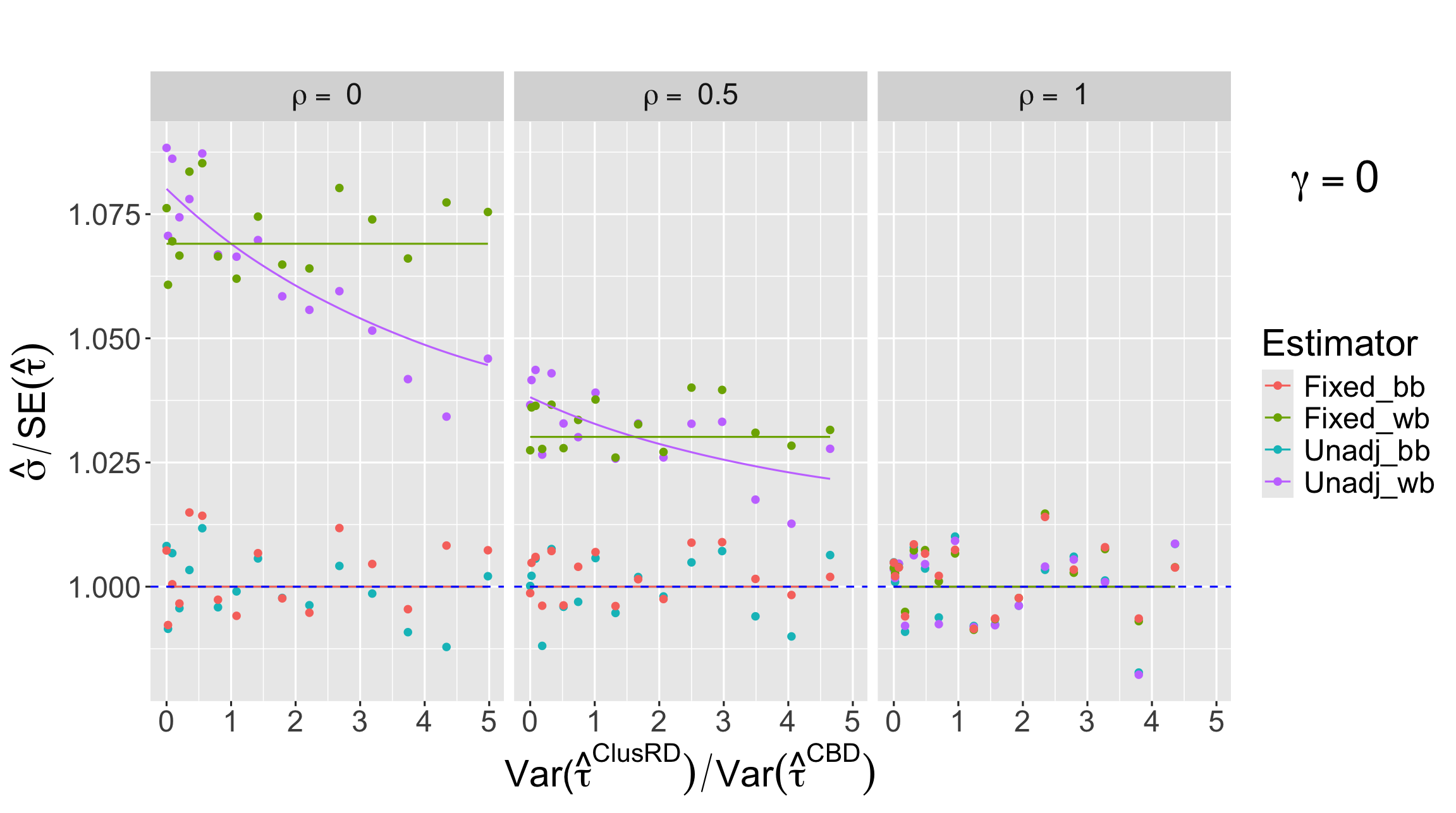
We present the results in Figure 1. The x-axis shows the ratio of variance between-blocks vs within-blocks, short-handed as the ratio of variance for a ClusRD vs a CBD as we saw these variances exactly capture these different components of variability in Section 4.1. Note that in S1 implying and in S2 implying . Recall from Section 4.1, when we should expect the difference in precision between a BIBD and a CRD to have the same sign as the difference in precision between a BIBD and a CBD; otherwise the sign of the comparison with CRD will be the opposite of the comparison with CBD. We see indeed that in S1, a BIBD is beneficial compared to both a CRD and a CBD when the ratio of variability of outcomes between vs within blocks is small. However, in S2, the BIBD is beneficial compared to a CRD when the ratio of between vs within variability is large.
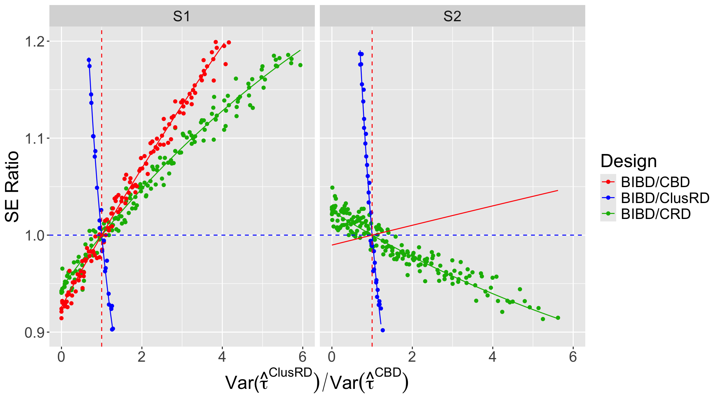
To aid in interpretation of the results, recall that the ratio of between and within variability should be 1 (denoted by the dotted vertical line on the figures) when blocking is done randomly (i.e., is uncorrelated with outcomes). Under S1, we see that the BIBD is advantageous compared to the CBD and the CRD when there is low between-block heterogeneity relative to within-block heterogeneity. However, compared to the ClusRD, the BIBD does worse when there is low between-block heterogeneity relative to within-block heterogeneity. We clearly see that the BIBD is a middle ground between the CBD and the ClusRD. Thus, when we believe units are relatively homogenous within blocks but heterogenous between blocks (i.e., we are blocking on a covariate that is predictive of outcome), we would prefer a CBD if it were possible to run. However, if a CBD were not possible in this case, a BIBD would yield notably better precision than a ClusRD. If we know that blocks are actually quite similar to each other, for example if they were formed with the goal of having similar distributions of units within each block, then a BIBD will actually outperform a CBD in terms of precision but we can do even better with a ClusRD. If we are uncertain about whether the blocks are better than random, in the sense of having lower within block relative to between block heterogeneity, a BIBD might be a good compromise between a CBD and a ClusRD in terms of precision.
Under S1, the comparison between the BIBD and the CRD is quite similar to that of a CBD. However, from Section 4.1, we have shown that this is not always the case. The results for S2 in Figure 1 illustrates how the story of comparing the BIBD to the CRD can flip due to the relative size of the blocks. Under S2, the BIBD is now more advantageous, compared to the CRD, when there is less heterogeneity within blocks and more heterogeneity between blocks. So depending on the size of the blocks, the benefits of the BIBD compared to the CRD may follow the usual intuition of the benefits of a CBD compared to a CRD, in that making units more homogenous within blocks is beneficial, or may follow the opposite of this. We note that the comparison with a ClusRD follows the same pattern, in terms of when it is beneficial, under S1 and S2 and, indeed, if a CBD were possible under S2 it would follow the same pattern as it exhibited under S1 as shown by the theoretical line under S2.
5.2 Comparison between BIBD estimators
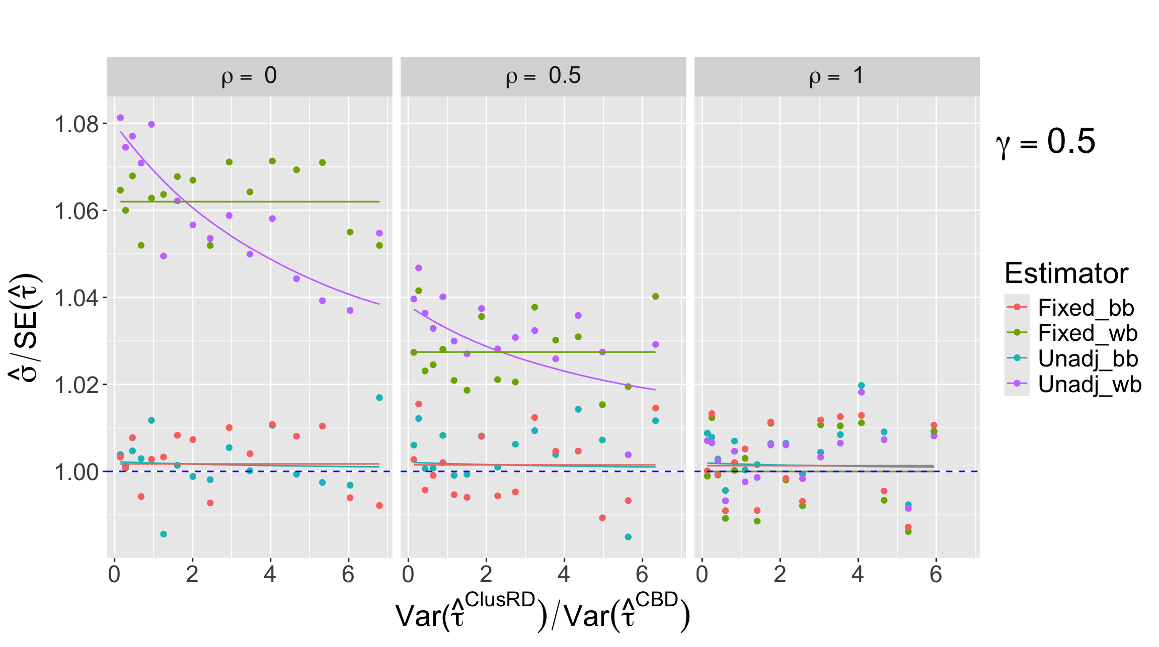
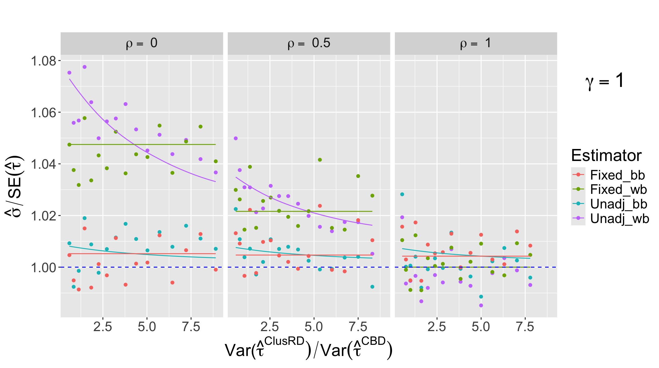
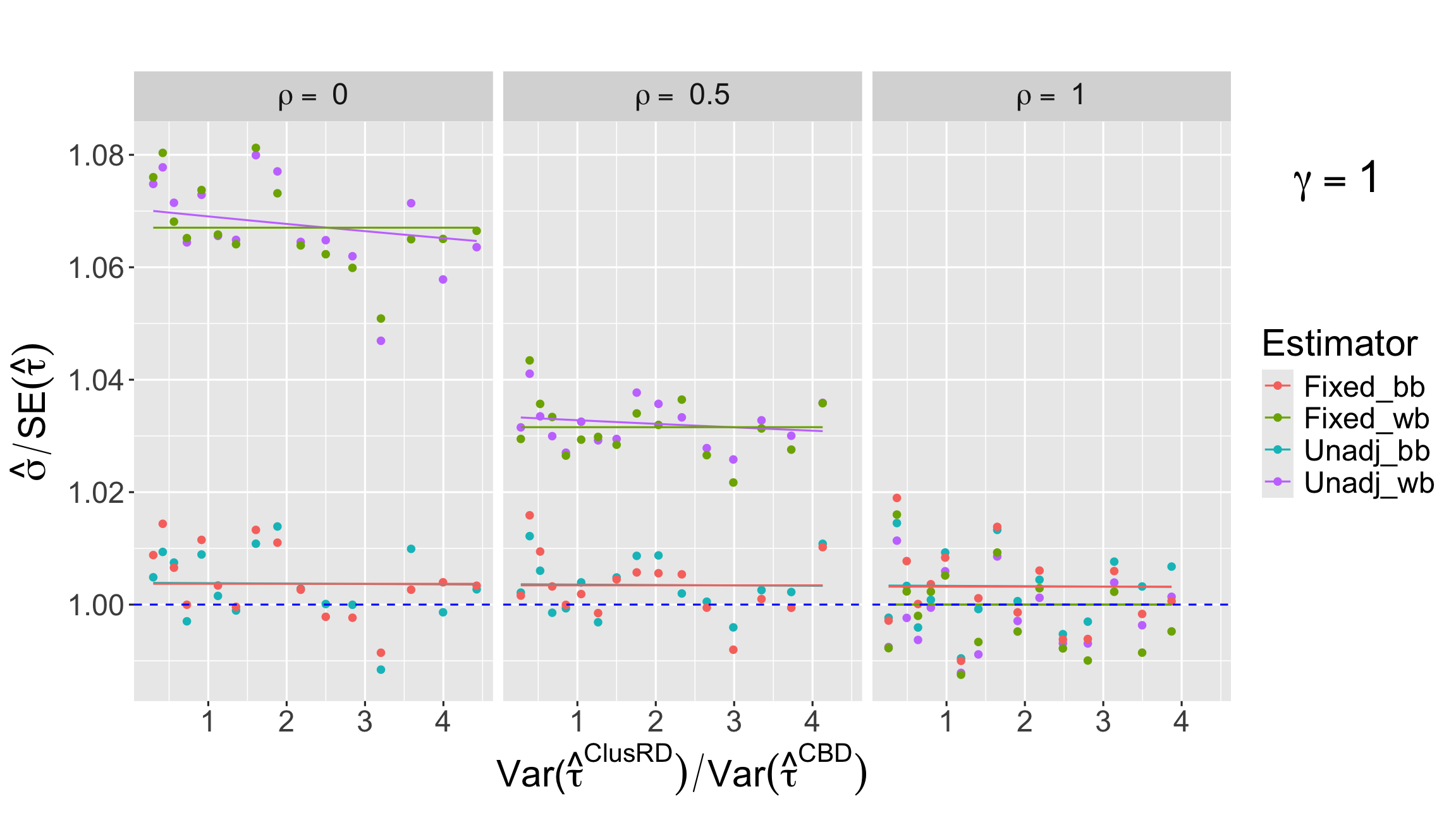
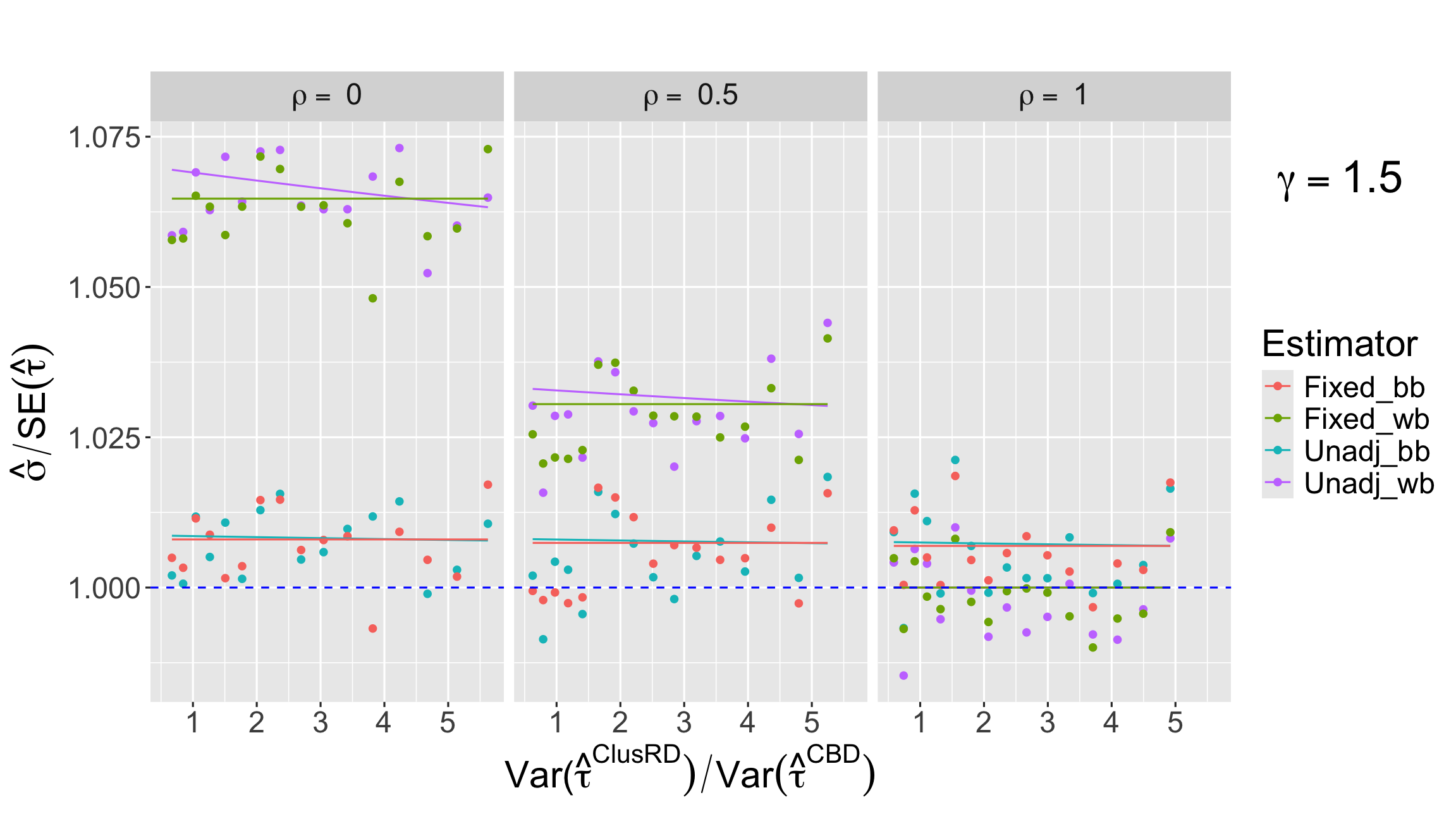
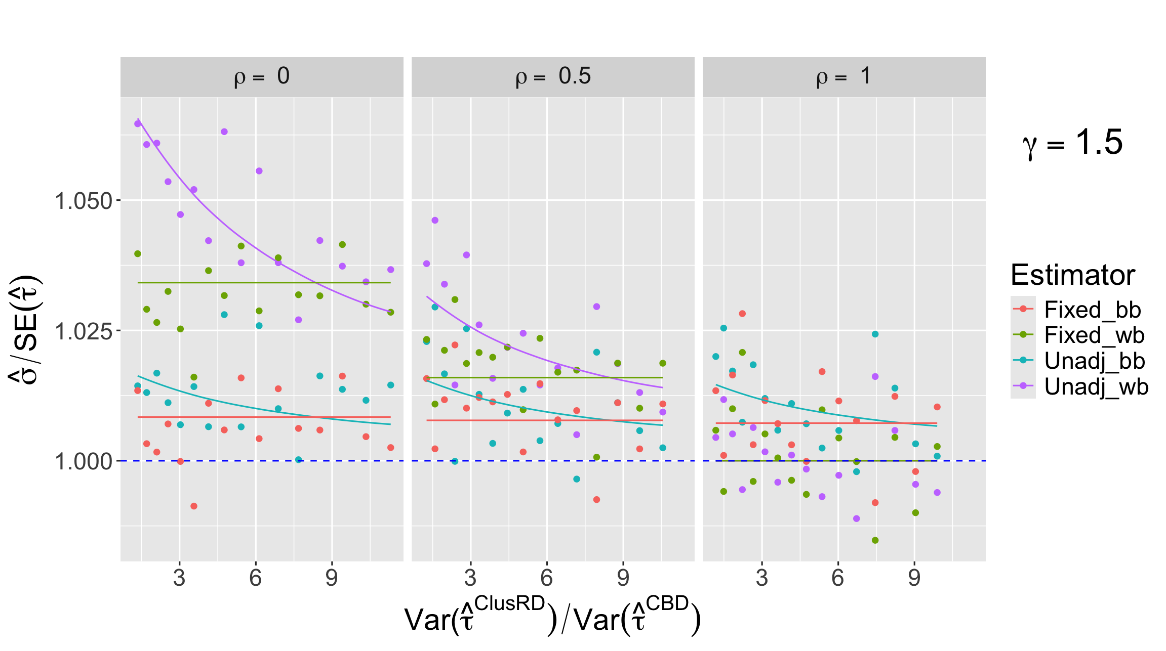
We now consider a comparison of the standard error of the unadjusted estimator, , and the fixed-effects style estimator, . For simplicity, we focus on S1 as our setting and results for S2, which largely follow a similar pattern, can be found in Supplementary Material C.1. The results are presented in Figure 2.
First consider the case when , recalling that this implies that the potential outcomes are generated following the fixed-effects model. As discussed in Section 4.2, the precision of depends on the correlation of potential outcomes, denoted by . In Figure 2, we see that under the values of considered, the fixed-effects estimator performs relatively better in terms of variability when the between-block variability is low compared to within-block variability, matching the intuition from Section 4.2 and the form of the variance. However, when exactly has an advantage compared to depends on . With uncorrelated potential outcomes (), there simply needs to be more between-block variability relative with within-block variability than expected by random blocking (which is when the between and within variability would be equal). This aligns with the results from Section 4.2. However, with additive effects () or partial correlation between potential outcomes (), we need higher between-block heterogeneity, relative to to within-block heterogeneity, for to be beneficial compared to .
Second, consider when is not zero, implying that the potential outcomes are generated following the interactive model. In this model, represents the level of interaction between the treatment and block. In Figure 2, we can see that performs better than in terms of precision as the size of the interaction increases. This aligns with the intuition that the fixed-effects style estimator should perform poorly when the outcomes do not follow a fixed-effects model. For example, when , even very high between block heterogeneity does not lead to being advantageous compared to . See Supplementary Material B.9 for mathematical justification of when the unadjusted estimator is more precise than the fixed-effects estimator in the case that within-block and between-block variability are equal (the red dashed line).
Overall, these simulations show the possibility of precision gains using compared to when the fixed-effects model holds and the blocking is lowering within-block variability compared to between-block variability. However, this advantage quickly disappears when the model is interactive and when there is a higher level of correlation between the potential outcomes. Because the blocks do not contain all treatments, an assumption of no interaction is not empirically testable. This leads us to recommend the unadjusted estimator as potential having relatively better precision across a larger variety of scenarios. We also note that simply calculating estimates of the effect based on both estimators and picking the one with smallest standard error estimates can lead to systematically anti-conservative inference.
5.3 Comparison between the variance estimators
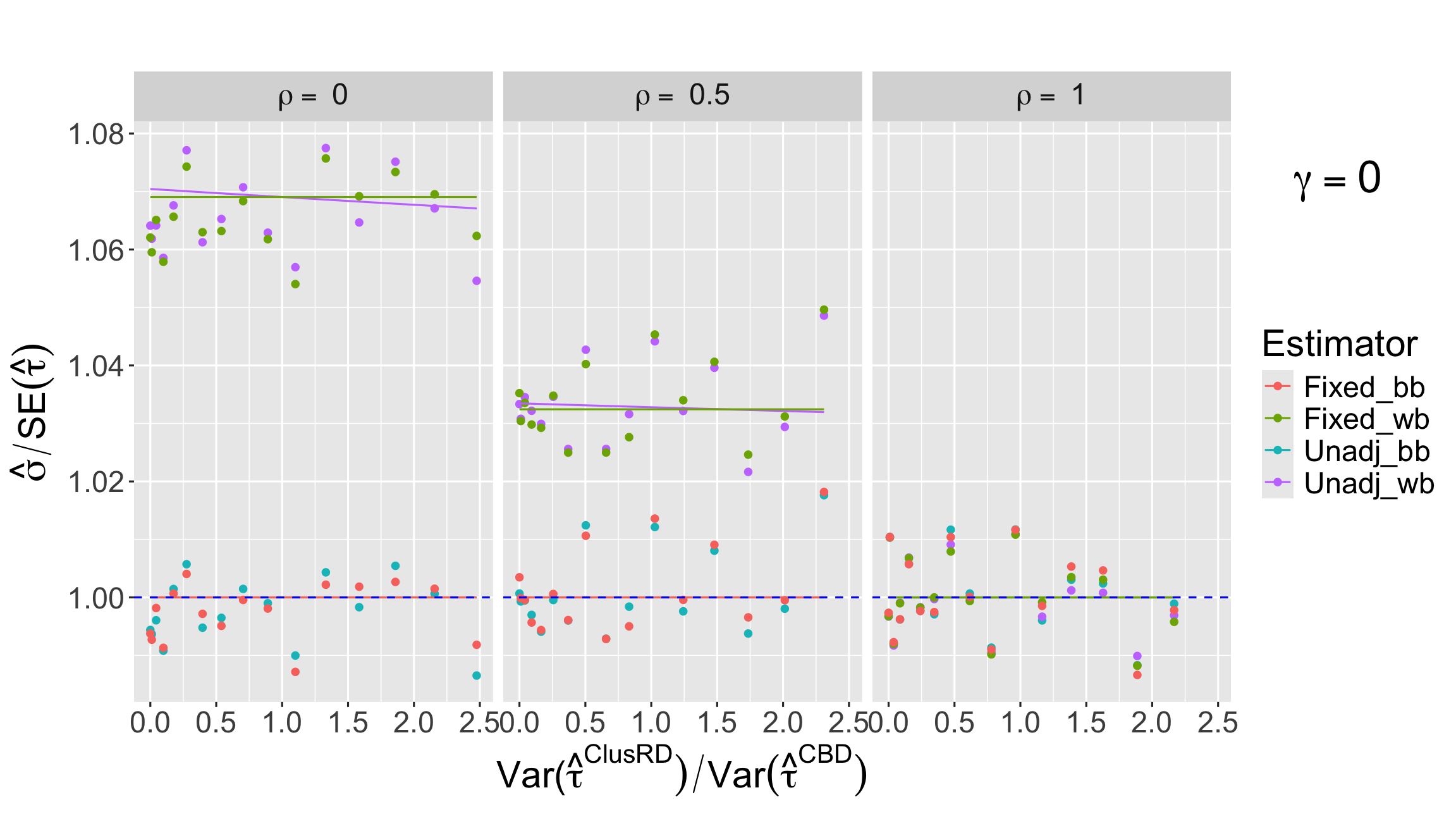
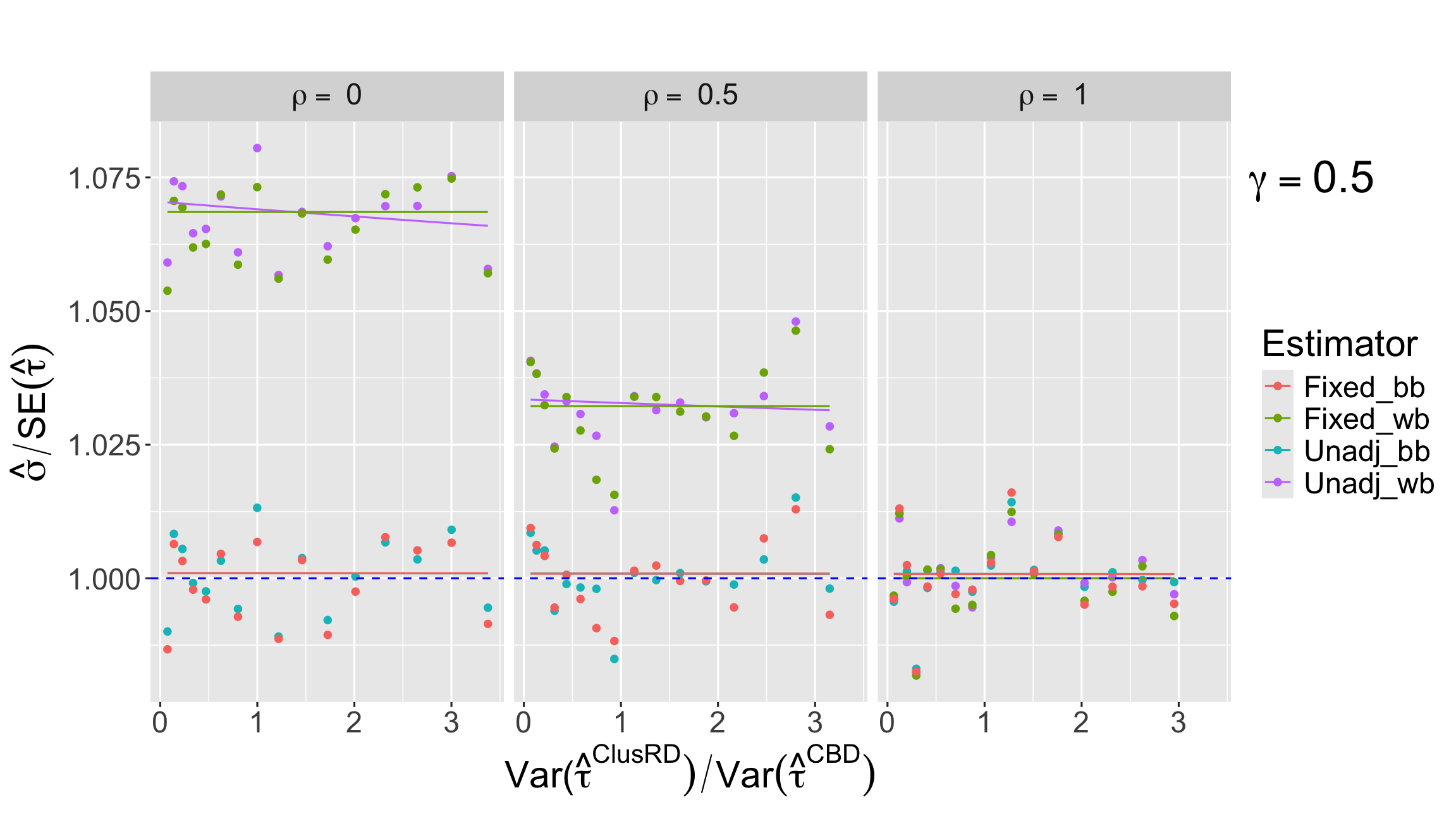
We conclude the simulation studies by considering a comparison of the variance estimators of and . We focus here on S1 with and as our setting, and the results are presented in Figure 3 and Figure 4 respectively. Additional results for other parameter settings in S1 and for S2 can be found in Supplementary Material C.2. In those additional results the overall patterns are similar, though under S2 the biases of the variance estimators of are flatter as increases, compared to the results under S1 below.
When , and are unbiased estimators of and because as discussed in Section 4.2. In Figure 3, we see that the variance estimators with an extra between-block term are less biased than those with an extra within-block term. However, as increases, the advantage of using and instead of and decreases. When effects are additive (), between-block and within-block heterogeneity are both zero, so all variance estimators are unbiased. Because the variance of the fixed-effects estimator only depends on between-block variability in terms of treatment variability, the biases of the fixed-effects variance estimators are constant for each and as values change (corresponding to changes in the x-axis of the figure). On the other hand, increases as increases. So, is decreasing function of when heterogeneity within blocks is fixed.
Next consider when , with results shown in Figure 4. In this setting, the common bias of and is no longer zero. Once again, the bias fixed-effects variance estimator does not change for given and . This is because the between-block variability terms of only depend on the interaction term, not the block effect term as we see in Section 4.2. As in the case with , the benefit of using and over and diminishes as increases. For the additive treatment effect case (), and are actually unbiased whereas and are not.
6 Data illustration
We revisit the Tennessee ’s student/teacher achievement ratio (STAR) Project (Word et al.,, 1990) to give an illustration of the use of BIBDs. The data is openly available (Achilles et al.,, 2008, https://doi.org/10.7910/DVN/SIWH9F). This study examined the impact of the following three treatments on educational achievement of elementary school students in Tennessee: small size classes (13-17 students per teacher), regular size classes (22-25 students per teacher), and regular size classes with a full-time teacher aide. A cohort of students in kindergarten in 1985-86 in 79 different schools were randomized into one of the three treatment conditions, which the students were then kept in through grade 3, with the exception of some switching of students in regular-sized classes into or out of classes with a teachers aide between kindergarten and first grade333There was also some movement of students into and out of schools.. A CBD was used with school as blocks. Thus, in order to participate, schools needed at least 57 students enrolled in kindergarten so that they could form at least one small class and two regular classes. In total, there were 328 kindergarten classrooms in the study. The researchers chose a CBD to mitigate variability due to between-school differences and also argue that ensuring each school experienced all three treatment incentivized full participation and mitigated potential biases (see, Word et al.,, 1990, for more). However, use of a BIBD with only two treatments assigned within each school could have allowed researchers to use a larger sample size by relaxing the enrollment requirement somewhat, thereby allowing more schools to participate.
In our re-analysis, we focus on the impact of first grade classroom assignment on the average of first grade Stanford Achievement Test (SAT) scores, where we average each student’s scores on the four test components (reading, math, listening, and word study skills) and then aggregate to the classroom level, which is our unit of analysis. We specifically compare small classes to regular classes (without aide). For simplicity of the illustration, we remove student entries with missing data for test scores, first grade classroom type, or school, which resulted in only 71 schools that had data available for classrooms in all three conditions. A BIBD with three total treatments and two assigned within each school (block) requires the total number of schools be a multiple of three. Further, within each school, there must be an equal number of classes (units) assigned to each condition. To mimic a BIBD, we (i) randomly drop two schools, (ii) randomly assign each of the remaining schools a pair of treatments, ensuring 23 schools get each pair of assignments (ii) randomly drop the minimum necessary classrooms so that each school has an equal number of classes assigned to each treatment. We can then apply our estimators for the treatment effect and variance. This was repeated 100 times to get an average over the noise in estimates due to the dropping of schools and classrooms. Results are presented as the first row in Table 4.
Because some schools had only one classroom per treatment, the within-block variance estimators are not applicable. To illustrate the within-block variance estimators, we subset to the 16 schools that are “big” (i.e., have at least two classrooms assigned to each treatment). We repeat the previous procedure of randomly dropping one school, randomly assigning block treatments, and randomly dropping classrooms as needed. These results, averaged over the random process completed 100 times, are presented as the second row in Table 4. As a further comparison, the CBD subsetted to the same set of 71 or 16 schools, but without dropping schools or classrooms, yields point estimates of 11.45 and 18.33, respectively, for the average block-level treatment effects. These estimates are fairly close to those from the BIBDs.
| Design | ||||||
|---|---|---|---|---|---|---|
| All blocks | 11.38 | N/A | 16.67 | 11.45 | N/A | 12.35 |
| Only “big” blocks | 18.08 | 73.75 | 67.35 | 18.98 | 36.84 | 30.44 |
The averaged estimated variability for the fixed-effects estimator is smaller than that for the unadjusted estimators, especially for the analysis with only “big” blocks. Although the variance estimators are biased (conservative), this gives some indication that the fixed-effects estimator had lower variance. Based on the results in the prior section, we expect the fixed-effects estimator to have lower variance when the block means differ across blocks but there is less variability within blocks. In this context, this would mean schools may have different average test scores and there may be variability within schools, but there is relatively less variability in average effects across schools. Further, the within-block variance estimators are larger than the between-block variance estimators for both estimators in the “big” block analysis. Based on the form of the bias of these variance estimators, this may indicate larger within-block than between-block heterogeneity of outcomes.
It is also notable that the estimate of the treatment effect changes quite a bit when only “big” blocks are used versus when all blocks are used. This further supports the notion that there is heterogeneity across schools. In particular, it appears that the treatment of smaller classrooms has a larger impact in bigger schools. One hypothetical explanation for this could be that resources in bigger schools might, in general, by shared by more students compared to smaller schools, making small classrooms with more focused attention and resources even more effective.
7 Discussion
We have explored BIBDs from the design-based potential outcome framework. These designs are useful when there are many treatments of interest and a CBD cannot be run. We focus on pairwise comparisons of two treatments in this setting. We proposed two unbiased estimators, an unadjusted estimator and a fixed-effects estimator, and found their variance under the finite-population setting. Further, we developed two variance estimators for each point estimator to use for conducting inference. This is, to our knowledge, the first development for BIBDs under the design-based potential outcome framework and thus broadens the range of tools researchers have at their disposable to design experiments and draw causal conclusions from them.
In addition to developing the basic inferential framework, we also compare BIBDs to common alternative designs. We find that the variance of the unadjusted estimator under a BIBD will always lie between the variance for a CBD and a ClusRD. In general, the ordering of variance will be CBD BIBD ClusRD when units are similar within blocks but there is heterogeneity across blocks. As the typical goal of blocking is to group units that are more similar, this implies that a BIBD can take advantage of some of the benefits of blocking, compared to a ClusRD, when a CBD is not feasible. On the other hand, if blocks are similar to other blocks on average but there is heterogeneity of outcomes within blocks, we will have CBD BIBD ClusRD. Although this scenario seems less common, it could occur when blocks are formed with the purpose of having similar distributions of units, which might happen for example in classrooms. Interestingly, if this is the case a simpler ClusRD is preferred. The comparison of BIBDs to CRDs is more nuanced, depending on the size of blocks and number of treatments.
The simulations demonstrate the relative performance of the different designs as well as the different estimators. When comparing the unadjusted estimator to the fixed-effects estimator, we find the unadjusted estimator performs well, in terms of precision, across a range of settings. We note that the fixed-effects estimator has an advantage when the fixed-effects model holds, potential outcomes are uncorrelated, and blocking reduces within-block heterogeneity. Without the assumption of a fixed-effects model and uncorrelated potential outcomes, the reduction of within-block heterogeneity compared to between-block heterogeneity needs to be more substantial for the fixed-effects model to have an advantage. Given this better robustness of the unadjusted estimator, we recommend the unadjusted estimator in general when there is uncertainty about the fixed-effects assumption. We note that picking the estimator with the lower observed variance can lead to anti-conservative inference and is therefore not recommended. Similarly, there are trade-offs between using a variance estimator that has a bias related within-block vs between-block heterogeneity that need to be weighed prior to seeing the data.
We demonstrate the estimation framework we developed through an illustration with data from the Tennessee STAR Project (Word et al.,, 1990). The original design was a CBD with schools as blocks, but we recreate what a BIBD may have looked like and show that the point estimates obtained are similar to the CBDs. Further, the estimated variances indicate high between-block variability in outcomes compared to within-block variability.
Although we have developed a solid framework for analysis of these designs under the design-based perspective, there are many avenues of further development. One important extension is moving from block-level to unit-level estimands and estimators. This will require incorporation of random weights to account for the random number of units assigned to each treatment condition, similar to weights needed for unit-level analysis in ClusRD (Middleton and Aronow,, 2015; Schochet et al.,, 2022). Similarly, it would be useful to extend this framework to more general incomplete block designs beyond BIBDs, which would allow more flexibility in use of these designs (e.g., would allow us to avoid the dropping strategy in the data illustration). Another direction is to extend the inference results to general contrast estimators that could be used for, e.g., factorial effects. Development of a finite-population central limit theorem for this design is also of interest and could be used to consider additional trade-offs of the various designs through changes in degrees of freedom of the associated inference.
References
- Abramson et al., (2022) Abramson, S. F., Koçak, K., and Magazinnik, A. (2022). What do we learn about voter preferences from conjoint experiments? American Journal of Political Science, 66(4):1008–1020.
- Achilles et al., (2008) Achilles, C., Bain, H. P., Bellott, F., Boyd-Zaharias, J., Finn, J., Folger, J., Johnston, J., and Word, E. (2008). Tennessee’s Student Teacher Achievement Ratio (STAR) project. https://doi.org/10.7910/DVN/SIWH9F.
- Bansak et al., (2018) Bansak, K., Hainmueller, J., Hopkins, D. J., and Yamamoto, T. (2018). The number of choice tasks and survey satisficing in conjoint experiments. Political Analysis, 26(1):112–119.
- Blackwell and Pashley, (2023) Blackwell, M. and Pashley, N. E. (2023). Noncompliance and instrumental variables for factorial experiments. Journal of the American Statistical Association, 118(542):1102–1114.
- Bose and Nair, (1939) Bose, R. C. and Nair, K. R. (1939). Partially balanced incomplete block designs. Sankhyā: The Indian Journal of Statistics (1933-1960), 4(3):337–372.
- Branson et al., (2016) Branson, Z., Dasgupta, T., and Rubin, D. B. (2016). Improving covariate balance in factorial designs via rerandomization with an application to a New York City Department of Education high school study. The Annals of Applied Statistics, 10(4):1958–1976.
- Cochran and Cox, (1957) Cochran, W. and Cox, G. (1957). Experimental Designs. Wiley New York, 2nd edition.
- Dasgupta et al., (2015) Dasgupta, T., Pillai, N. S., and Rubin, D. B. (2015). Causal inference from factorial designs by using potential outcomes. Journal of the Royal Statistical Society: Series B, 77(4):727–753.
- Dean et al., (2017) Dean, A., Voss, D., and Draguljić, D. (2017). Design and Analysis of Experiments. Springer.
- Egami and Imai, (2018) Egami, N. and Imai, K. (2018). Causal interaction in factorial experiments: Application to conjoint analysis. Journal of the American Statistical Association, 114(526):529–540.
- Fisher and Yates, (1953) Fisher, R. A. and Yates, F. (1953). Statistical tables for biological, agricultural, and medical research. Hafner Publishing Company.
- Fogarty, (2018) Fogarty, C. B. (2018). On mitigating the analytical limitations of finely stratified experiments. Journal of the Royal Statistical Society Series B: Statistical Methodology, 80(5):1035–1056.
- Gerber and Green, (2012) Gerber, A. and Green, D. (2012). Field Experiments: Design, Analysis, and Interpretation. W. W. Norton.
- Goplerud et al., (2022) Goplerud, M., Imai, K., and Pashley, N. E. (2022). Estimating heterogeneous causal effects of high-dimensional treatments: Application to conjoint analysis. arXiv preprint arXiv:2201.01357.
- Graham and Cable, (2001) Graham, M. E. and Cable, D. M. (2001). Consideration of the incomplete block design for policy-capturing research. Organizational Research Methods, 4(1):26–45.
- Hainmueller et al., (2014) Hainmueller, J., Hopkins, D. J., and Yamamoto, T. (2014). Causal inference in conjoint analysis: Understanding multidimensional choices via stated preference experiments. Political Analysis, 22(1):1–30.
- Imai, (2008) Imai, K. (2008). Variance identification and efficiency analysis in randomized experiments under the matched-pair design. Statistics in medicine, 27(24):4857–4873.
- Imai et al., (2008) Imai, K., King, G., and Stuart, E. A. (2008). Misunderstandings between experimentalists and observationalists about causal inference. Journal of the Royal Statistical Society: Series A, 171(2):481–502.
- Imbens and Rubin, (2015) Imbens, G. W. and Rubin, D. B. (2015). Causal inference in statistics, social, and biomedical sciences. Cambridge University Press.
- Kempthorne, (1956) Kempthorne, O. (1956). The Efficiency Factor of an Incomplete Block Design. The Annals of Mathematical Statistics, 27(3):846 – 849.
- Li and Ding, (2017) Li, X. and Ding, P. (2017). General forms of finite population central limit theorems with applications to causal inference. Journal of the American Statistical Association, 112(520):1759–1769.
- Li et al., (2020) Li, X., Ding, P., and Rubin, D. B. (2020). Rerandomization in factorial experiments. The Annals of Statistics, 48(1):43–63.
- Liu et al., (2024) Liu, H., Ren, J., and Yang, Y. (2024). Randomization-based joint central limit theorem and efficient covariate adjustment in randomized block factorial experiments. Journal of the American Statistical Association, 119(545):136–150.
- Liu and Yang, (2020) Liu, H. and Yang, Y. (2020). Regression-adjusted average treatment effect estimates in stratified randomized experiments. Biometrika, 107(4):935–948.
- Lu, (2016) Lu, J. (2016). Covariate adjustment in randomization-based causal inference for factorial designs. Statistics & Probability Letters, 119:11–20.
- Middleton and Aronow, (2015) Middleton, J. A. and Aronow, P. M. (2015). Unbiased estimation of the average treatment effect in cluster-randomized experiments. Statistics, Politics and Policy, 6(1-2):39–75.
- Mukherjee and Ding, (2019) Mukherjee, R. and Ding, P. (2019). Latin square designs: Causal inference in a potential outcomes framework. In Proc. 62nd ISI World Statistics Congress, volume 1 of Contributed Paper Session, Kuala Lumpur, Malaysia. Department of Statistics Malaysia (DOSM). https://isi2019.org/proceeding/3.CPS/CPS%20VOL%201/index.html.
- Oehlert, (2010) Oehlert, G. W. (2010). A first course in design and analysis of experiments.
- Pashley and Bind, (2023) Pashley, N. E. and Bind, M.-A. C. (2023). Causal inference for multiple treatments using fractional factorial designs. Canadian Journal of Statistics, 51(2):444–468.
- Pashley and Miratrix, (2021) Pashley, N. E. and Miratrix, L. W. (2021). Insights on variance estimation for blocked and matched pairs designs. Journal of Educational and Behavioral Statistics, 46(3):271–296.
- Pashley and Miratrix, (2022) Pashley, N. E. and Miratrix, L. W. (2022). Block what you can, except when you shouldn’t. Journal of Educational and Behavioral Statistics, 47(1):69–100.
- Rubin, (1980) Rubin, D. B. (1980). Randomization analysis of experimental data: The Fisher randomization test comment. Journal of the American Statistical Association, 75(371):591–593.
- Sailer, (2005) Sailer, O. (2005). Crossdes: A package for design and randomization in crossover studies. R News, 5:24–27. https://journal.r-project.org/articles/RN-2005-018/.
- Schnitzer et al., (2016) Schnitzer, M. E., Steele, R. J., Bally, M., and Shrier, I. (2016). A causal inference approach to network meta-analysis. Journal of Causal Inference, 4(2).
- Schochet, (2013) Schochet, P. Z. (2013). Estimators for clustered education rcts using the neyman model for causal inference. Journal of Educational and Behavioral Statistics, 38(3):219–238.
- Schochet et al., (2022) Schochet, P. Z., Pashley, N. E., Miratrix, L. W., and Kautz, T. (2022). Design-based ratio estimators and central limit theorems for clustered, blocked rcts. Journal of the American Statistical Association, 117(540):2135–2146.
- Su and Ding, (2021) Su, F. and Ding, P. (2021). Model-assisted analyses of cluster-randomized experiments. Journal of the Royal Statistical Society Series B: Statistical Methodology, 83(5):994–1015.
- Word et al., (1990) Word, E., Johnston, J., Bain, H. P., Fulton, B. D., Zaharias, J. B., Achilles, C. M., Lintz, M. N., Folger, J., and Breda, C. (1990). The state of tennessee’s student/teacher achievement ratio (star) project. Tennessee Board of Education.
- Wu and Hamada, (2021) Wu, C. J. and Hamada, M. S. (2021). Experiments: Planning, Analysis, and Optimization. John Wiley & Sons, 3rd edition.
- Wu and Gagnon-Bartsch, (2021) Wu, E. and Gagnon-Bartsch, J. A. (2021). Design-based covariate adjustments in paired experiments. Journal of Educational and Behavioral Statistics, 46(1):109–132.
- (41) Zhao, A. and Ding, P. (2022a). Reconciling design-based and model-based causal inferences for split-plot experiments. The Annals of Statistics, 50(2):1170–1192.
- (42) Zhao, A. and Ding, P. (2022b). Regression-based causal inference with factorial experiments: estimands, model specifications and design-based properties. Biometrika, 109(3):799–815.
- Zhao et al., (2018) Zhao, A., Ding, P., Mukerjee, R., and Dasgupta, T. (2018). Randomization-based causal inference from split-plot designs. The Annals of Statistics, 46(5):1876–1903.
Supplementary Material
for
“Causal Inference for Balanced Incomplete Block Designs”
These supplementary materials are organized as follows: Section A provides useful expressions and expansions that are used in the proofs. Section B provides proofs of the results in the main paper. Section C provides additional simulation results.
Appendix A Useful expressions
A.1 Probabilities for treatment assignments and block membership
For a BIBD, as defined in the main paper, we provide the following simplifications of probabilities related to assigning treatment to the blocks.
For ,
For , recall that we denote the “membership” type of block based on treatments assigned to it as
Then
Recall also that for
and
Further, let
Let be the number of blocks containing and , but not , and be the number of blocks containing , , and , but not for . Then, because blocks contain and not , and . So,
Analogous expressions hold for conditioning on by replacing with .
For block and such that ,
A.2 Variance and covariance of indicators of block membership
For ,
A.3 Useful simplifications of quadratic sums
Derivation of the finite-population variances involves quadratic sums, so we provide a couple of simplifications of these types of expressions below:
Appendix B Proofs
B.1 Proof of Theorem 3.1
Here we prove unbiasedness of the unadjusted estimator: .
Proof.
To make always well defined, take if . Conditional on being assigned to block ,
By the law of iterated expectation,
Thus, . ∎
B.2 Proof of Theorem 3.2
We show here the derivation of the variance of the unadjusted estimator,
Proof.
We first set up some useful notation. Recall
and let , , and .
With this notation and using the simplifications from Section A.3,
Recall the standard variance decomposition,
The conditional expectation is
Using Theorem 3 of Li and Ding, (2017) and noting that ,
Because and by the conditions for a BIBD,
On the other hand, the conditional variance of our estimator is
by Theorem 3 of Li and Ding, (2017). The expectation of this conditional variance is then
Let
Then, putting the variance of the conditional expectation and the expectation of the conditional variance together, we can write
∎
B.3 Proof of Theorem 3.3
In this section we derive the expectation of the variance estimators for the unadjusted estimator, and , recalling
Proof.
We begin by finding the expectation of the variance estimator components and .
We start with the conditional expectation of ,
By the law of iterated expectation, taking the expectation over ,
Similarly,
For , conditional on , this is a standard variance estimator with known expectation, . Then it’s easy to see that .
Applying these simplifications, we have
To make the bias of the estimators nonnegative, we add either a within-block term (for ) or a between block term (for ); the biases of these terms, respectively, are
Thus,
∎
B.4 Proof of Theorem 3.4
Here we prove unbiasedness of the fixed-effects style estimator: .
Proof.
Using the notation , , and defined previously, we can write
Its expectation is
The first term is
For the second term (and similarly the third term),
because . Thus,
The last two lines simplify because and . Therefore is an unbiased estimator of . ∎
B.5 Proof of Theorem 3.5
We show here the derivation of the variance of ,
Proof.
We will use the same decomposition of variance as in Section B.2, into the expectation of the conditional variance and the variance of the conditional expectation. We start with the conditional variance of , which is
We know that
For and , consider
where . By Theorem 3 of Li and Ding, (2017),
where
By taking the expectation over ,
Thus,
| (S4) | |||
| (S5) |
Now consider the conditional expectation.
Now we have a format for the conditional variance to apply Theorem 3 of Li and Ding, (2017). To help see the connection to that result better, we can conceptualize a hypothetical experiment. Consider an experiment with potential outcomes
Note that the ’s are fixed functions of potential outcomes (i.e., not random). Keep the probability of a block having , , , etc. the same as our original BIBD. Then we can write the conditional variance above as
This is a the variability of a contrast of “observed” means from the hypothetical experiment described above, making Theorem 3 of Li and Ding, (2017) directly applicable.
By Theorem 3 of Li and Ding, (2017),
Note that there are there are an equal number of across type B and type C blocks so portion of the last term is 0. Further, recall definitions
Then we can simplify further,
We provide some simplification of the constants below using the relations and :
So we have for the variance of the conditional expectation
| (S6) |
The overall variance, adding the variance of the conditional expectation from (S6) and the expectation of the conditional variance from (S5), is then
∎
B.6 Proof of Theorem 3.6
Here we derive the bias of and , recalling
Proof.
Recall from Section B.3,
Applying these results to the components of the variance estimators,
where and are defined in Section 3.2. Thus,
As in Section B.3, we add terms
for or
for so that the biases of variance estimator are nonnegative. Therefore, the biases of our variance estimators are
∎
B.7 Expectation of variability over random blocking
In this section we derive the expectation of variance components if blocking is done at random (i.e., outcomes are uncorrelated with blocks). Consider if we blocked units into blocks at random, fixing the block size . Let be the indicator that unit was assigned to block (). In this scenario the ’s are random variables and we assume the probability of each unit being assigned to a particular block is . Let and . We have
and
It is useful to note that
We first find the expectation of over the random blocking:
Next find the expectation of over the random blocking:
So we see that
B.8 Role of block size in comparison of BIBDs to CRDs
Recall in Section 4.1 we showed that, under the condition ,
where
In this section, we explore when the sign of is positive or negative. First, we check when , which is the smallest block size for a BIBD. In this case,
because .
Thus, when , we always have and the BIBD will be beneficial compared to CRD when units are more similar within each block than between blocks.
More generally, we see that is an increasing function in provided that is fixed, and for
In particular, and if , and otherwise. Again, the BIBD will be beneficial compared to the CRD when units are more similar within each block than between blocks when the block size is small such that . In the big block size case (), the BIBD will be beneficial compared to the CRD when units are more similar across blocks than within block.
B.9 Comparison of unadjusted estimators to fixed-effects estimators
We first consider the case where the potential outcomes follow the linear fixed-effects relationship given in Section 4.2. As a reminder, the model is
for unit with , and we take . Recall this implies
Thus, for ,
First, consider again the assumption that potential outcomes are independent in the sense that , so that for all . We compare the precision of and in terms of and , which correspond to the between-block and within-block variability, respectively, for . Under the same potential outcomes model assumptions above independent potential outcomes, when
When ,
Thus, when , with the equality holding when . We see this exact result in Figure 2.
Alternatively, in this model, without the assumption of independent potential outcomes, the between block component of vanishes. However, the between block component of is
If we assume for all and for some constant for all , the within block component of is
Under the same assumption,
so the within block component of is
Thus, holds when
Because
the above inequality can be reduced as
So, we can say that holds when
We remark that is an increasing function of and . Also, when . When , we can directly compare the precision of and with the ratio of between block variance to within block variance. In particular, when random blocking occurs, then as we have shown, so we expect that the precision of two estimators will be similar. However, when , unlike the comparisons discussed in Section 4.1, this means that even if random blocking occurs, the relationship between the precision of the unadjusted estimator and the fixed-effects estimator can change depending on the correlation of potential outcomes, . For example, when , so we should expect that random blocking would lead to higher precision of the fixed-effects estimator compared to the unadjusted estimator.
We can also consider model misspecification of the fixed-effects estimator. For example, we can assume of the following interactive fixed-effects model:
for unit with . We make the same assumptions on the correlation of potential outcomes as before. Then, for , and are the same as above, but
As discussed in the main text, this means that the between block component of the variance of the fixed-effects estimator increases because the terms are no longer zero under this assumption. In this model,
where . Thus, does not depend on .
Appendix C Additional simulation results
In this section, we present additional simulation results.
C.1 Additional results for the comparison between BIBD estimators
We provide results for the comparison of the unadjusted and fixed-effects estimators under setting S2 in Figure 5. The results are largely the same as those under S1 discussed in Section 5.2. In particular, the fixed effects estimator will perform based on when there is no interactive effect, low correlation of potential outcomes, and high between block versus within block variability. We note that the potential benefits of of the fixed-effects estimator seem to diminish more quickly as the correlation increases, compared to S1.
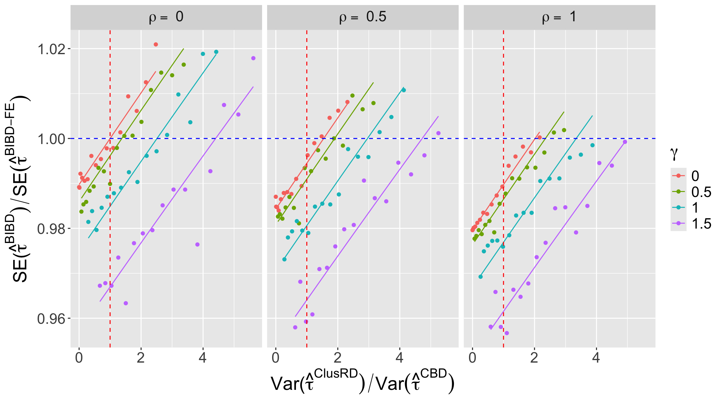
C.2 Additional results for the comparison between the variance estimators
We provide additional results for the comparison of the bias of the variance estimators under different simulations settings. Figures 6 and 7 give results for S1 with and , respectively. Figures 8, 9, 10, and 11 give results for S2 with , , and , respectively. The results largely follow those shown in Section 5.3. For within-block variance estimators, it is the size of the correlation between potential outcomes that matters for bias, with unbiasedness achieved when , i.e., additive effects within blocks. For between-block variance estimators, the largest driver of bias is the size of , which controls the variability of effects across blocks, with unbiasedness occuring when .
In contrast to S1, the percent bias of the variance estimator of under S2 does not decrease much as increases, which is similar to the percent bias of the variance estimator of . The smaller change in bias under S2 is an artifact of the difference between the two settings in number of total treatments and number of treatments within each block, which impacts the magnitude of the true variance as a function of the ratio of within-block and between-block variability.