The Effect of Tornadic Supercell Thunderstorms on the Atmospheric Muon Flux

Abstract

Tornadoes are severe weather phenomena characterized by a violently rotating column of air connecting the ground to a parent storm. Within the United States, hundreds of tornadoes occur every year. Despite this, the dynamics of tornado formation and propagation are not particularly well understood, in part due to the challenge of instrumentation: many existing instruments for measuring atmospheric properties are in-situ detectors, making deployment in or near an active or developing tornado difficult. Here, we combine local atmospheric and cosmic ray air shower simulation to explore the potential for remote measurement of the pressure field within tornado-producing supercell thunderstorms by examining directional variations of the atmospheric muon flux.

I Introduction

I.1 Tornadoes

Tornadoes are violently rotating columns of air connecting a cumuliform cloud with the ground. Though tornadoes are relatively common in the United States, the process by which they form is currently not well understood, though significant efforts in theoretical and computational modeling as well as field observations have advanced our understanding a great deal. It is known that the strongest, longest-lived tornadoes form from supercell thunderstorms, defined by the presence of a persistent, rotating updraft. Ground level rotation is intensified by an upward-directed pressure gradient force, converging and amplifying vertical vorticity and producing a region of intense circulation [1].

Recent simulations of tornado formation suggest the presence of a low pressure core in the parent supercell thunderstorm that contributes to tornado formation [2], however experimental measurements of this region are logistically difficult. Current pressure field measurements rely on deploying instrumentation in the path of an approaching storm [3]. This method can be unreliable, as it requires a tornado to track near the pre-deployed sensors, and strong tornadoes may damage or destroy the instrument. Surface-based measurements are also only able to measure the pressure field at ground level, concealing variations in the pressure field with altitude. Drone and aircraft based measurements can measure the pressure field as at function of altitude [4], but these measurements are restricted to the immediate vicinity of the instrument itself, making measurements over large volumes and within turbulent weather systems difficult.

I.2 Atmospheric Muons

Cosmic rays are charged particles (protons, as well as heavier atomic nuclei) accelerated in faraway astrophysical sources. Though the exact origins of cosmic rays remain an open question in astrophysics, their flux at Earth is well measured [5]. Cosmic rays that reach Earth can interact with nuclei in the atmosphere, producing a shower of secondary particles. This particle shower includes pions and kaons, which will eventually decay, producing muons:

$$\pi^{\pm}\rightarrow\mu^{\pm}+\overset{\textbf{(---)}}{\nu}_{\mu}$$ (1)

$$K^{\pm}\rightarrow\mu^{\pm}+\overset{\textbf{(---)}}{\nu}_{\mu}$$ (2)

Muons also lose energy as they propagate through matter. Their energy losses can be described by:

$$\frac{dE}{dx}=\rho(x)[a(x,E)+E*b(x,E)]$$ (3)

where E is the energy of the muon, $x$ is the distance traveled, $\rho(x)$ is the density of the traversed matter and $a(x,E)$, $b(x,E)$ are the ionisation and radiative energy losses. The quantities $\rho$, $a$, and $b$ are all dependent on the properties of the matter traversed. For atmospheric muons, $\rho$ is directly proportional to the atmospheric pressure [6].

Muons eventually decay, producing electrons and neutrinos:

$$\mu^{-}\rightarrow e^{-}+\bar{\nu}_{e}+\nu_{\mu}$$ (4)

$$\mu^{+}\rightarrow e^{+}+\nu_{e}+\bar{\nu}_{\mu}$$ (5)

Muons have a lifetime of approximately 2.2 $\mu s$ in the rest frame [5]. In the frame of the surface of the Earth, energetic muons are time dilated, allowing them to travel significant distance ($\approx$10s to 100s of kilometers) into the atmosphere before decaying. Higher energy muons are able to travel farther prior to decaying, and in combination with the energy losses due to matter described above, this means that the overall atmospheric muon flux is effectively attenuated by matter.

In the past, this effect has been leveraged as a probe of matter density along the muon path. A muon detector is placed near an object of interest, and the flux of muons travelling through the object is measured and compared to a nominal flux of muons that did not pass through the object. The suppression of the muon flux observed travelling through the object is directly related to the integral of the density along the muon path. This technique (“muon tomography”) has previously been used in a variety of contexts, including measurements of the interiors of volcanoes and the Great Pyramids [6].

The atmospheric muon flux is known to be proportional to the local atmospheric pressure. This has been demonstrated to be true on large scales: daily and weekly variations in the atmospheric muon flux that are correlated with atmospheric pressure have been observed by various muon detectors [7][8]. On smaller scales, local variations in atmospheric pressure have been observed in data from muon telescopes pointed at typhoons off the coast of Japan [9], as well as non-tornadic thunderstorms [10][11].

Previous studies have also identified variations in the atmospheric muon flux associated with electric fields inside thunderstorms [12][10]. For the purposes of this paper, electric field effects are neglected, as we seek to explore solely the effect of the pressure field on the muon flux. In practice, however, both the pressure and electric field would need to be modeled to fully describe any potential real-world observations.

II Remote Sensing of Pressure Using Atmospheric Muons

II.1 Conceptual Overview

Since the atmospheric muon flux is correlated with the density of matter along the muon path, and the density of air in the atmosphere is correlated with the atmospheric air pressure, this implies that variations in atmospheric air pressure can be observed as variations in the atmospheric muon flux. A hypothetical muon detector could detect variations in air pressure as a function of altitude by measuring the muon flux at different zenith angles. As mentioned above, this has been done to measure the low pressure region of typhoons, where a region of increased muon flux was found to be correlated with the low-pressure regions of the target typhoon [9]. Given the success of this method in the context of typhoon measurements, we consider extending this technique to make a similar measurement of the pressure field within supercell thunderstorms.

In comparison to typhoons, supercell thunderstorms present several unique challenges. Supercell thunderstorms are significantly smaller than typhoons. While typhoons can grow to be hundreds of kilometers in diameter, supercell thunderstorms typically only occupy an area tens of kilometers in radius. The smaller physical scale of supercell thunderstorms translates to a smaller effect on the muon flux, as muons are in a low-density region for a smaller portion of their total propagation path. This manifests as a smaller difference in atmospheric muon flux when comparing the high and low pressure regions of the storm. Additionally, supercell thunderstorms evolve quickly, with lifetimes rarely exceeding 4 hours [13]. The short window of observation needed to observe the dynamics of these storms makes it difficult to collect enough muon data to observe small variations in the muon flux. This effect can be mitigated by simply constructing a larger muon detector, as this allows for a larger number of muon counts to be observed over the same time period. Thus, there are two important questions that we seek to answer:

• Given an estimate of the pressure perturbations within a supercell thunderstorm, how large is the corresponding effect on the atmospheric muon flux?

• How large of a muon detector is needed to observe an effect of this scale on reasonable ($\approx$hour) time scales?

For the purposes of this study, a setup similar to that described in [9] is simulated. A muon detector is simulated on the ground 10 kilometers from the center of a thunderstorm. Cosmic ray showers are generated in the upper atmosphere, and propagated through the thunderstorm to the location of our muon detector. The observed number of muon counts over 1 hour is recorded along various lines of sight leading to the detector, producing a “map” of muon counts as a function of elevation ($\theta$) and azimuthal ($\phi$) angle. A similar map is assembled using the same setup without the presence of a thunderstorm, and the two maps are compared to determine the effect of the storm on the atmospheric muon flux.

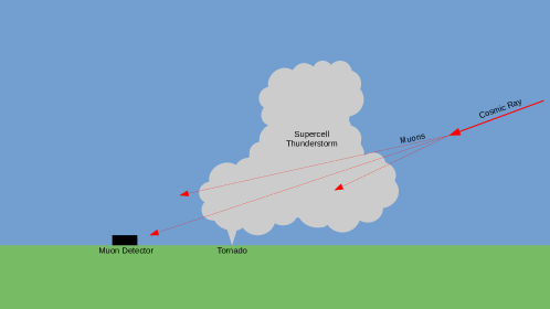
Figure 1: A cartoon of the setup considered in this paper (not to scale). Cosmic rays interact in the upper atmosphere, and secondary muons propagate through a supercell thunderstorm. A muon detector is placed on the opposite side of the storm, and the effect of the thunderstorm pressure field on the flux of atmospheric muons is calculated.

II.2 Supercell Thunderstorm Simulation

Cloud Model 1 (CM1), a three-dimensional nonhydrostatic fully compressible cloud model, was used to simulate the tornadic supercell thunderstorm [14]. Among the prognostic variables CM1 solves for include wind, potential temperature, pressure, turbulent kinetic energy, and water substance including water vapor, cloud water, cloud ice, rain, snow, graupel and hail. For the purpose of this study, only the pressure field was analyzed. The initial environmental conditions for the simulation were identical to [15] and [16], namely, the state of the atmosphere prior to the observed 24 May 2011, El Reno, Oklahoma supercell that produced a long-track violent tornado. Physics parameterization options for the simulation include three-moment microphysics [17] and a subgrid turbulent kinetic energy closure scheme [18]. The simulation utilized an isotropic cubic mesh with a grid spacing of 75 m, and was triggered using an updraft nudging technique [19]. The simulation morphology is similar to [15], with the storm initially splitting with a dominant right-moving supercell (analyzed herein) producing a vigorous low-level rotating updraft (mesocyclone) prior to the formation of a violent tornado. The pressure field of the storm is analyzed at two model times: after the formation of the low-level mesocyclone but prior to tornado formation ($t=3600$ s) and during the strongest phase of the tornado ($t=8760$ s).

II.3 Muon Simulation

MCEq is used to numerically solve the atmospheric particle cascade equations describing the muon flux as the atmospheric shower propagates through the atmosphere. The primary cosmic ray flux is simulated according to the model described in [20]. Primary cosmic ray interactions are then simulated using the SIBYLL 2.3c interaction model [21]. The resultant muon flux is then propagated through an atmospheric model described in the previous section.

A simulated muon detector is placed at the origin, with local atmospheric variations obtained from the model described in the previous section simulated in a 37.5 km (length) $\times$ 37.5 km (width) $\times$ 28.05 km (height) box surrounding the detector. Outside this region we use a standard unperturbed atmospheric model identical to the US standard atmosphere implemented in CORSIKA, originally parameterized by J. Linsley [22].

The combined number of $\mu^{+}$ and $\mu^{-}$ counts for each $2\times 2$ degree angular bin in $\theta$ and $\phi$ is calculated by integrating the muon flux. The calculations presented here assume a muon detector with perfect efficiency ($\epsilon=1.0$). Modern muon detectors have been shown to have efficiencies of at least $\epsilon=0.5$ [23][24][25]. Smaller muon detection efficiencies would introduce a factor of $\epsilon$ to equations 6 and 7. Using $\Phi_{0}$ to denote the muon flux under an unperturbed (no-storm) atmosphere, the nominal expected number of events would then be:

$$N_{exp}(\theta_{bin},\phi_{bin})=\int_{E_{min}}^{E_{max}}\int_{\Delta\phi}\int_{\Delta\theta}\Phi_{0}(\theta,\phi,E)\,d\Omega dE$$ (6)

Where $\Delta\theta$ and $\Delta\phi$ correspond to the size of the angular bins in azimuth and elevation (2 degrees). The bounds of the energy integral, $E_{min}$ and $E_{max}$ describe the minimum and maximum muon energies that were simulated. For this paper, muon fluxes were calculated between $E_{min}=0\text{ TeV}$ and $E_{max}=10^{8}\text{ TeV}$, however the vast majority ($>99\%$) of the atmospheric muon flux exists between 0 and 100 TeV. To give a sense of scale: for a 1000 square meter muon detector, the expected rate of atmospheric muons is approximately 28,400 events per square degree angular bin per hour at $\theta=40^{\circ}$. This rate varies naturally as a function of elevation angle, with a lower flux near the horizon and a higher flux from very vertical elevation angles [26].

A expectation of the observed number of counts can be calculated by integrating the muon flux resulting from simulating the atmospheric model described in the previous section ($\Phi_{storm}$):

$$N_{obs}(\theta_{bin},\phi_{bin})=\int_{E_{min}}^{E_{max}}\int_{\Delta\phi}\int_{\Delta\theta}\Phi_{storm}(\theta,\phi,E)\,d\Omega dE$$ (7)

Poisson variations are added to $N_{obs}$ to simulate real data. Since the muon rate varies by several orders of magnitude as a function of elevation angle, it is convenient to work with a poisson likelihood describing the probability of observing $N_{obs}$ counts from a particular direction:

$$L(N_{obs})=\int_{-\infty}^{N_{obs}}P(N_{exp},x)dx$$ (8)

where $P(N_{exp},x)$ is a poisson distribution with mean $N_{exp}$, obtained from equation 6. This normalizes the resultant maps of the muon flux to the expected rate under an unperturbed atmosphere at a particular elevation angle so muon paths at different elevation angles are easier to compare.

III Results

Figure 2 shows the idealized expectation of the effect of the storm pressure field on the atmospheric muon flux along various lines of sight for a 1000 m² muon detector. Regions of increased muon flux, identifiable as groups of pixels with higher values of $L$, correspond to low-pressure regions of the storm. Similarly, regions of suppressed muon flux correspond to higher-pressure regions. Note, however, that the muon flux is correlated with the average of the pressure field along a particular line of sight, meaning information about the pressure field as a function of depth is not easily accessible from the two dimensional images shown. Depth-dependent information about the pressure field could conceivably be obtained by multiple detectors with different views of the same storm, or by examining the energy distribution of detected muons, however development of this idea is left for future study.

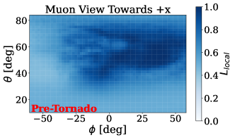
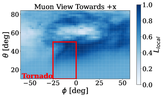
Figure 2: Idealized (without Poisson noise) expectations of the effect of a supercell thunderstorm on the atmospheric muon flux. Top: a muographic image of a storm prior to tornado formation. Bottom: a muographic image of a storm containing a tornado, with the region containing an active tornado outlined by a red box.

To obtain realistic examples of 1 hour exposures, poisson variations are added to $N_{obs}$ and $L$ is recalculated using the new values. Examples of maps of $L$ containing these variations can be seen in figure 3. Near the horizon, the muon flux is lower and the data is dominated by poisson variations. At high elevations ($\theta>30$ degrees) the structure of the high and low pressure regions of the storm begin to become visible as clusters of pixels with lower/elevated $L$ values.

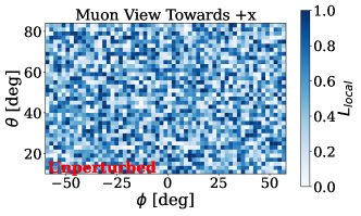
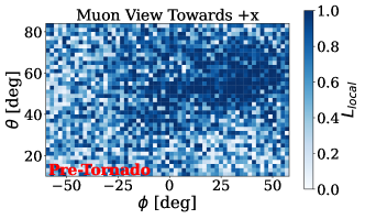
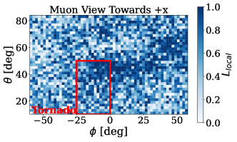
Figure 3: “Realistic” expectations of the effect of a supercell thunderstorm on the atmospheric muon flux. Top: a muographic image of an unperturbed atmosphere. Middle: a muographic image of an active storm prior to tornado formation. Bottom: a muographic image of a storm containing a tornado with the region containing an active tornado outlined by a red box.

The large scale variation of the muon flux variations can be more easily seen if the noisy maps of $L$ are passed through a filtering algorithm that averages together pixels within 20 degrees of one another. This smooths out small scale poisson variations, allowing the larger scale evolution of the pressure field to be examined. We select a filtering radius of 20 degrees, as this is the point at which the integral described in equation 6 produces $N_{obs}\approx 10^{6}$ events, suggesting that variations on the scale of 1% can be measured when comparing angular bins of this size. Examples of filtered maps of $L$ can be seen in figure 4. For comparison, a maps of $L$ corresponding to an unperturbed atmosphere with no storm present is also shown.

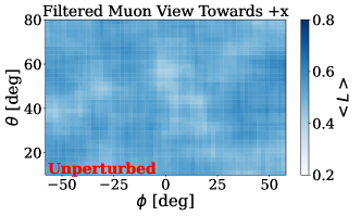
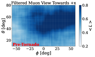
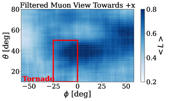
Figure 4: Filtered versions of the noisy maps shown in figure 3. Pixels within 20 degrees of one another are averaged, smoothing out small scale noise variations. Top: The filtered map of an unperturbed atmosphere. Middle: The filtered map of a storm prior to tornado formation. Bottom: The filtered map of a storm containing a tornado. The “true” position of the tornado is shown as a red box. The filtering technique smoothes over small scale variations within this region, however the parent low pressure core of the storm is still clearly visible.

Muographic images of a target storm may be noisy, however model-based methods may be able to identify structure on relatively small ($\approx$ 1 km) length scales. If the general shape of a tornado in the pressure field is known, the location of the tornado can be recovered from a noisy map of the muon flux with a simple cross correlation. Figure 5 shows the idealized (noiseless) expectation of the effect of an active tornado on the atmospheric muon flux observed by a 1000 m² detector. This “tornado template” is cross-correlated along the $\phi$ axis with a noisy realization of simulated data. Using this technique, the presence of a tornado can be determined, even in the presence of significant statistical fluctuations. Though this scenario is optimistic due to the assumption of exact prior knowledge of the pressure field, it suggests the potential for model-based unfolding of the underlying atmospheric pressure field from atmospheric muon observations.

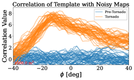
Figure 5: Left: The template of the idealized effect of a tornado on the local muon flux. Right: The cross correlation along $\phi$ of the tornado template with noisy $L$ maps, for both simulation of a storm with (orange) and without (blue) a tornado present using a 50 m² muon detector.

IV Discussion

IV.1 Muon Detector Size

The previous studies presented in this paper use a fairly large 1000 m² muon detector as a baseline. There are several existing cosmic ray detectors of this scale or larger that are sensitive to the atmospheric muon flux [27][28]. (Un)fortunately, there have been no recorded tornadoes in the vicinity of either of these detectors, as they are not located in particularly tornado-active regions [29]. Given that tornado detection often relies on eyewitness observation, and that these detectors are in remote locations, it is possible that tornadoes occurred near these detectors but were not officially recorded. If this is the case, an investigation into historical muon data from these detectors could reveal a signature corresponding to a previously unidentified tornado.

Smaller detectors may still be able to measure atmospheric pressure effects on the muon flux. Since variations in the atmospheric muon flux due to supercell thunderstorms are on the order of 1%, muon detectors seeking to measure this effect need to be large enough to collect O($10^{6}$) atmospheric muon counts over the angular area of interest during the lifetime of the storm (typically 10s to 100s of minutes). Measurements taken with smaller detectors will have larger relative statistical fluctuations, making it more difficult to identify the underlying structure of the pressure field. On the other hand, smaller detectors also have the potential to be significantly more portable. While a 1000 m² would likely need to be a permanent, stationary installation, a 100 m² detector could conceivably be moved to a location with projected severe weather within the next few days, and a 50 m² detector is small enough to fit on roughly 5 trucks, allowing for the detector to be moved to the location of a severe weather event as it is developing. Examples of filtered maps of muon data taken by 100 m² and 50 m² detectors can be seen in figure 6. Though statistical variations conceal much of the structure seen in figure 4, the effect of the tornado on the underlying pressure field can still be observed in the cross correlations of the noisy muon maps with a template describing the tornado pressure field, albeit to a much smaller degree. This is shown in figure 7.

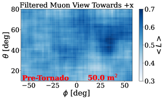
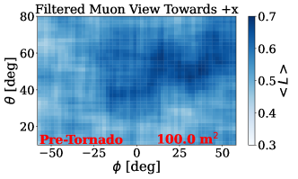
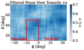
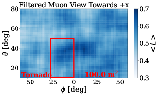
Figure 6: Filtered maps of the atmospheric muon flux for 50 m² (left) and 100 m² (right) detectors. Elevated atmospheric muon flux can be observed in the region containing a tornado, however the effect is significantly reduced in comparison with the 1000 m² case

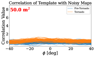
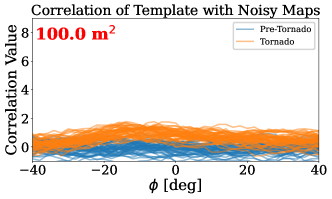
Figure 7: Plots of the cross correlation of a tornado template with noisy maps of $L$ both pre- and post-tornado formation as in figure 5, but using realizations of data from 50 m² (top) and 100 m² (bottom) detectors.

IV.2 Range and Resolution

Though individual pressure measurements using this technique may not be as precise in measuring the pressure at a particular location when compared to more traditional in-situ methods, there is a distinct advantage in being able to remotely measure the pressure field over large distance scales. Measurements of the atmospheric muon flux can reveal unique information of the variation of the pressure field as a function of height that is inaccessible to ground-based pressure sensors. Additionally, the lack of a need for in-situ instrumentation makes this measurement more logistically straightforward than current methods, as it does not require detectors to be within the direct path of an active tornado.

The range of this technique depends on the desired spatial resolution of the pressure perturbation field. The atmospheric muon flux naturally varies with elevation angle, with a higher proportion of muon events incident at large elevation angles [26]. For a fixed detector size, a more detailed scan of the pressure field requires a larger number of muon counts, which can be obtained by using the muon flux a higher (more vertical) elevation angles. However, using data at higher elevation angles reduces the maximum possible horizontal distance between the detector and the storm.

To calculate the resolution of this technique, we require an observation of $10^{6}$ events within an angular radius of $\Delta\psi$ degrees (the “resolution” of this technique). We assume that the error on reconstructing the directions of individual muon events is small relative to $\Delta\psi$, though in practice this will depend on the specifics of the detector. We can compute the range of this technique ($R$) for a particular desired distance scale and elevation angle with the following geometric relation:

$$R=\frac{d}{\text{tan}(\Delta\psi)}\text{cos}(\theta)$$ (9)

Where $d$ is the distance scale over which pressure variations are measured, $\theta$ is the elevation angle of the target region, and $\Delta\psi$ is obtained for a particular elevation angle from the curves shown in figure 8. Due to the competing effects of the increased resolution at low elevation angles, and the decreased horizontal distance when examining high elevation angles, the horizontal range of this technique peaks near an elevation angle of 45 degrees. This can be seen for various detector sizes and desired distance resolutions in figure 9. Note that here “horizontal range” is the distance along the surface of the Earth (i.e. how far you would have to drive to be directly below the target location).

With a 1000 m² muon detector, a 5 kilometer resolution measurement of the pressure field could be obtained at a distance of up to 35 kilometers, though this is restricted to along the $\theta=40^{\circ}$ line of sight. If a larger, permanent muon detector were placed in a tornado-prone location, this would translate to being able to measure the pressure field of $O(1)$ tornadoes every year [29]. Smaller detectors would have a reduced, but still significant range, capable of measuring pressure variations over 5 kilometer length scales at a range of 10 kilometers. Such detectors would have the important advantage of portability, with the potential to be deployed or moved near regions expected to experience severe weather in the near future.

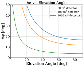
Figure 8: The angular bin size required to capture $10^{6}$ muons at various elevations angles and various detector sizes. Since the muon flux decreases for small elevation angles, larger angular bins are needed to capture a fixed number of muons. This translates to concealing variations in the muon flux on small length scales in these regions, as there is an insufficient density of muons to measure these effects.

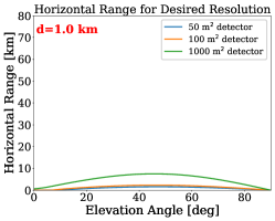
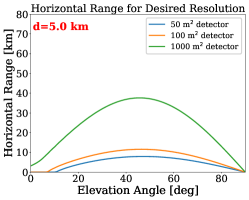
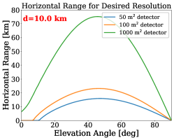
Figure 9: Projected horizontal ranges of using this technique to measure pressure field variations along the listed length scales ($d$). Large elevation angles correspond to a higher muon rate allowing for more precise measurements, but also geometrically correspond to a smaller horizontal distance to a particular altitude layer. These two competing effects are roughly balanced near an elevation angle of 45 degrees, where the horizontal range of this technique is maximized.

IV.3 Other Weather Phenomena

In the more general case, atmospheric phenomena can be characterized by their physical size and the scale of their pressure perturbations. By simulating various atmospheric phenomena described by these two variables, we can estimate what types of atmospheric phenomena are candidates for remote pressure measurements using atmospheric muons.

A simplified simulation of the pressure field is used to achieve this. Different atmospheric phenomena are simulated as 10-kilometer tall cylinders of negative pressure perturbation, with variable horizontal radius. The radius and average pressure perturbation are varied, and for each case the muon flux residual integrated over the full field of view is recorded. This can be used to estimate how large of an effect various atmospheric phenomena might have on the muon flux. These curves, as well as highlighted regions corresponding to different atmospheric phenomena, can be seen in figure 10. These results seem consistent with previous studies [9][11], which have observed perturbations in the muon flux in the vicinity of typhoons (hurricanes) and non-tornadic thunderstorms.

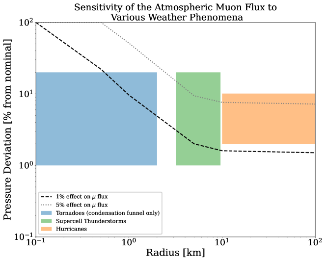
Figure 10: Various severe weather phenomena plotted in the space of size (x-axis), and magnitude of associated pressure drop (y-axis) [30][31][13][32][33]. Highlighted regions for tornadoes, thunderstorms, and hurricanes are approximate, as these values have not been exhaustively cataloged for the majority of storms. For the purposes of this plot, supercell thunderstorms are estimated to have pressure deviations comparable to that of tornadoes, though this has yet to be measured. Curves showing regions of a 1% and 5% effect on the atmospheric muon flux are shown, where points above these curves are expected to produce a larger deviation in the muon flux.

V Conclusion

Here we have presented simulations of the atmospheric muon flux in the presence of a supercell thunderstorm with an active tornado. We find that such a storm would introduce directional variations in the atmospheric muon flux of approximately 1%. If a storm can be observed over the course of an hour, a 1000 m² muon detector would likely be capable of measuring variations in the local pressure field over approximately 1 kilometer length scales. If a prior model for the pressure field associated with the tornado itself can be developed, this technique could additionally be used to identify the presence and location of an active tornado.

The 1000 m² muon detector considered in this paper is smaller than several existing cosmic ray telescopes. Detectors covering an even smaller area would likely be able to do similar science, and would have the advantage of portability, though will have to contend with proportionally larger statistical variations. In either case, measurements of the atmospheric muon flux in the vicinity of supercell thunderstorms could provide valuable information about the pressure field over a large volume that cannot be obtained using existing methods.

VI Acknowledgements

The authors are grateful for helpful discussions with John Beacom, Austin Cummings, Kaeli Hughes, Peter Taylor, Justin Flaherty and Paul Martini.

References

- Markowski and Richardson [2014] P. Markowski and Y. Richardson, What we know and don’t know about tornado formation, Physics Today 67, 26 (2014), https://pubs.aip.org/physicstoday/article-pdf/67/9/26/10100108/26_1_online.pdf .
- Orf et al. [2017a] L. Orf, R. Wilhelmson, B. Lee, C. Finley, and A. Houston, Evolution of a long-track violent tornado within a simulated supercell, Bulletin of the American Meteorological Society 98, 45 (2017a).
- Karstens et al. [2010] C. D. Karstens, T. M. Samaras, B. D. Lee, W. A. Gallus, and C. A. Finley, Near-ground pressure and wind measurements in tornadoes, Monthly Weather Review 138, 2570 (2010).
- Frew et al. [2020] E. W. Frew, B. Argrow, S. Borenstein, S. Swenson, C. A. Hirst, H. Havenga, and A. Houston, Field observation of tornadic supercells by multiple autonomous fixed-wing unmanned aircraft, Journal of Field Robotics 37, 1077 (2020), https://onlinelibrary.wiley.com/doi/pdf/10.1002/rob.21947 .
- Workman and Others [2022] R. L. Workman and Others (Particle Data Group), Review of Particle Physics, PTEP 2022, 083C01 (2022).
- Lechmann et al. [2021] A. Lechmann, D. Mair, A. Ariga, T. Ariga, A. Ereditato, R. Nishiyama, C. Pistillo, P. Scampoli, F. Schlunegger, and M. Vladymyrov, Muon tomography in geoscientific research – a guide to best practice, Earth-Science Reviews 222, 103842 (2021).
- Jourde et al. [2016] K. Jourde, D. Gibert, J. Marteau, J. de Bremond d’Ars, S. Gardien, C. Girerd, and J.-C. Ianigro, Monitoring temporal opacity fluctuations of large structures with muon radiography: a calibration experiment using a water tower, Scientific Reports 6, 10.1038/srep23054 (2016).
- Tilav et al. [2019] S. Tilav, T. K. Gaisser, D. Soldin, and P. Desiati, Seasonal variation of atmospheric muons in icecube (2019), arXiv:1909.01406 [astro-ph.HE] .
- Tanaka et al. [2022] H. Tanaka, J. Gluyas, M. Holma, J. Joutsenvaara, P. Kuusiniemi, G. Leone, D. Lo Presti, J. Matsushima, L. Oláh, S. Steigerwald, L. Thompson, I. Usoskin, S. Poluianov, D. Varga, and Y. Yokota, Atmospheric muography for imaging and monitoring tropic cyclones, Scientific Reports 12, 16710 (2022).
- Karapetyan [2014] G. G. Karapetyan, Variations of muon flux in the atmosphere during thunderstorms, Phys. Rev. D 89, 093005 (2014).
- Kozyrev et al. [2015] A. Kozyrev, N. Barbashina, T. Belyakova, J. Pavlyukov, A. Petrukhin, N. Serebryannik, V. Shutenko, and I. Yashin, Studies of thunderstorm events based on the data of muon hodoscope uragan and meteorological radar dmrl-c, Physics Procedia 74, 486 (2015), fundamental Research in Particle Physics and Cosmophysics.
- Abbasi et al. [2022] R. U. Abbasi et al. (Telescope Array), Observation of variations in cosmic ray single count rates during thunderstorms and implications for large-scale electric field changes, Phys. Rev. D 105, 062002 (2022).
- Davenport [2021] C. E. Davenport, Environmental evolution of long-lived supercell thunderstorms in the great plains, Weather and Forecasting 36, 2187 (2021).
- Bryan and Fritsch [2002] G. H. Bryan and J. M. Fritsch, A benchmark simulation for moist nonhydrostatic numerical models, Mon. Weather Rev. 130, 2917 (2002), http://dx.doi.org/10.1175/1520-0493(2002)130¡2917:ABSFMN¿2.0.CO;2 .
- Orf et al. [2017b] L. Orf, R. Wilhelmson, B. Lee, C. Finley, and A. Houston, Evolution of a Long-Track violent tornado within a simulated supercell, Bull. Am. Meteorol. Soc. 98, 45 (2017b).
- Orf [2019] L. Orf, A violently tornadic supercell thunderstorm simulation spanning a Quarter-Trillion grid volumes: Computational challenges, I/O framework, and visualizations of tornadogenesis, Atmosphere 10, 578 (2019).
- Mansell et al. [2010] E. R. Mansell, C. L. Ziegler, and E. C. Bruning, Simulated electrification of a small thunderstorm with Two-Moment bulk microphysics, J. Atmos. Sci. 67, 171 (2010).
- Deardorff [1980] J. W. Deardorff, Stratocumulus-capped mixed layers derived from a three-dimensional model, Boundary Layer Meteorol. 18, 495 (1980).
- Naylor and Gilmore [2012] J. Naylor and M. S. Gilmore, Convective initiation in an idealized cloud model using an updraft nudging technique, Mon. Weather Rev. 140, 3699 (2012).
- Gaisser [2012] T. K. Gaisser, Spectrum of cosmic-ray nucleons, kaon production, and the atmospheric muon charge ratio, Astroparticle Physics 35, 801 (2012), arXiv:1111.6675 [astro-ph.HE] .
- Riehn et al. [2018] F. Riehn, H. P. Dembinski, R. Engel, A. Fedynitch, T. K. Gaisser, and T. Stanev, The hadronic interaction model SIBYLL 2.3c and Feynman scaling, PoS ICRC2017, 301 (2018), arXiv:1709.07227 [hep-ph] .
- Heck et al. [1998] D. Heck, J. Knapp, J. N. Capdevielle, G. Schatz, and T. Thouw, CORSIKA: a Monte Carlo code to simulate extensive air showers. (1998).
- Park et al. [2023] C. Park, K. B. Kim, M. K. Baek, I. soo Kang, S. Lee, Y. S. Chung, H. Chung, and Y. H. Chung, Development of a muon detector based on a plastic scintillator and wls fibers to be used for muon tomography system, Nuclear Engineering and Technology 55, 1009 (2023).
- Pan [2004] M. Pan, Determining muon detection efficiency rates of limited streamer tube modules using cosmic ray detector, SLAC-TN-04-061 (2004).
- Anghel et al. [2015] V. Anghel, J. Armitage, F. Baig, K. Boniface, K. Boudjemline, J. Bueno, E. Charles, P.-L. Drouin, A. Erlandson, G. Gallant, R. Gazit, D. Godin, V. Golovko, C. Howard, R. Hydomako, C. Jewett, G. Jonkmans, Z. Liu, A. Robichaud, T. Stocki, M. Thompson, and D. Waller, A plastic scintillator-based muon tomography system with an integrated muon spectrometer, Nuclear Instruments and Methods in Physics Research Section A: Accelerators, Spectrometers, Detectors and Associated Equipment 798, 12 (2015).
- Gaisser [1990] T. K. Gaisser, Cosmic rays and particle physics. (1990).
- Aug [2015] Nuclear Instruments and Methods in Physics Research Section A: Accelerators, Spectrometers, Detectors and Associated Equipment 798, 172–213 (2015).
- Teshima [1997] M. Teshima (Telescope Array), Telescope Array project, in 32nd Rencontres de Moriond: High-Energy Phenomena in Astrophysics (1997) pp. 217–222.
- [29] Severe Weather Database (1950-2022), https://www.spc.noaa.gov/wcm/#data, accessed: 2024-03-01.
- Riehl [1950] H. Riehl, A Model of Hurricane Formation, Journal of Applied Physics 21, 917 (1950).
- Chavas and Knaff [2022] D. R. Chavas and J. A. Knaff, A simple model for predicting the tropical cyclone radius of maximum wind from outer size, Weather and Forecasting 37, 563 (2022).
- Brooks [2004] H. E. Brooks, On the relationship of tornado path length and width to intensity, Weather and Forecasting 19, 310 (2004).
- [33] HRD Hurricane Database, https://www.aoml.noaa.gov/hrd/hurdat/Data_Storm.html, accessed: 2024-03-01.