SDPRLayers: Certifiable Backpropagation Through Polynomial Optimization Problems in Robotics

Abstract

Differentiable optimization is a powerful new paradigm capable of reconciling model-based and learning-based approaches in robotics. However, the majority of robotics optimization problems are non-convex and current differentiable optimization techniques are therefore prone to convergence to local minima. When this occurs, the gradients provided by these existing solvers can be wildly inaccurate and will ultimately corrupt the training process. On the other hand, any non-convex robotics problems can be framed as polynomial optimization problems and, in turn, admit convex relaxations that can be used to recover a global solution via so-called certifiably correct methods. We present SDPRLayers, an approach that leverages these methods as well as state-of-the-art convex implicit differentiation techniques to provide certifiably correct gradients throughout the training process. We introduce this approach and showcase theoretical results that provide conditions under which correctness of the gradients is guaranteed. We demonstrate our approach on two simple-but-demonstrative simulated examples, which expose the potential pitfalls of existing, state-of-the-art, differentiable optimization methods. We apply our method in a real-world application: we train a deep neural network to detect image keypoints for robot localization in challenging lighting conditions. An open-source, PyTorch implementation of SDPRLayers will be made available upon paper acceptance.

I Introduction and Related Work

The versatility of learning models has made them ubiquitous in robotics, now appearing in almost all layers of the modern software stack [67]. On the other hand, model-based optimization – the mainstay of traditional robotics – provides a level of robustness, accuracy and generalization that has proven difficult to match by learning-based methods [55]. A new paradigm, leveraging advances in so-called differentiable optimizers, now enables roboticists to combine these two approaches into a single end-to-end learning framework.

In this approach, optimization problems are embedded as ‘layers’ in deep-learning networks, with optimization parameter data as the input and the optimal solution as the output. Similar to other layers in machine learning, the forward pass of the layer involves solving the optimization, while the backward pass computes the gradients. To date, the most effective way to perform the backward pass is to implicitly differentiate the conditions of optimality [8].

The benefits of this approach are several, allowing practitioners to capitalize on the respective advantages of model-based and learning approaches while also mitigating their disadvantages. For example, this integration means that domain knowledge can be injected directly into the robotics pipeline, while still allowing machine learning parameters to be trained on the final goal of a robotics module. This also obviates costly integration and fine-tuning stages that are necessary when learning and optimization modules are developed in parallel [67].

New tools geared towards differentiable optimization in a robotics setting have been recently presented. Theseus, developed by Pineda et al. [52], presents a differentiable optimization layer for unconstrained, non-linear least-squares problems that typically appear in robotics. Crucially, this tool builds off work by Teed and Deng [64] to solve problems with Lie Group constraints. PyPose further tailors differentiable optimization layers to robotics applications by exploiting the sparsity inherent within many problems, though it is not yet as versatile as Theseus [67]. For trajectory optimization, CALIPSO provides differentiable solutions using an interior-point solver and is able to handle conic and complementarity constraints, which often occur when dealing with friction and contact in robotic motion [36].

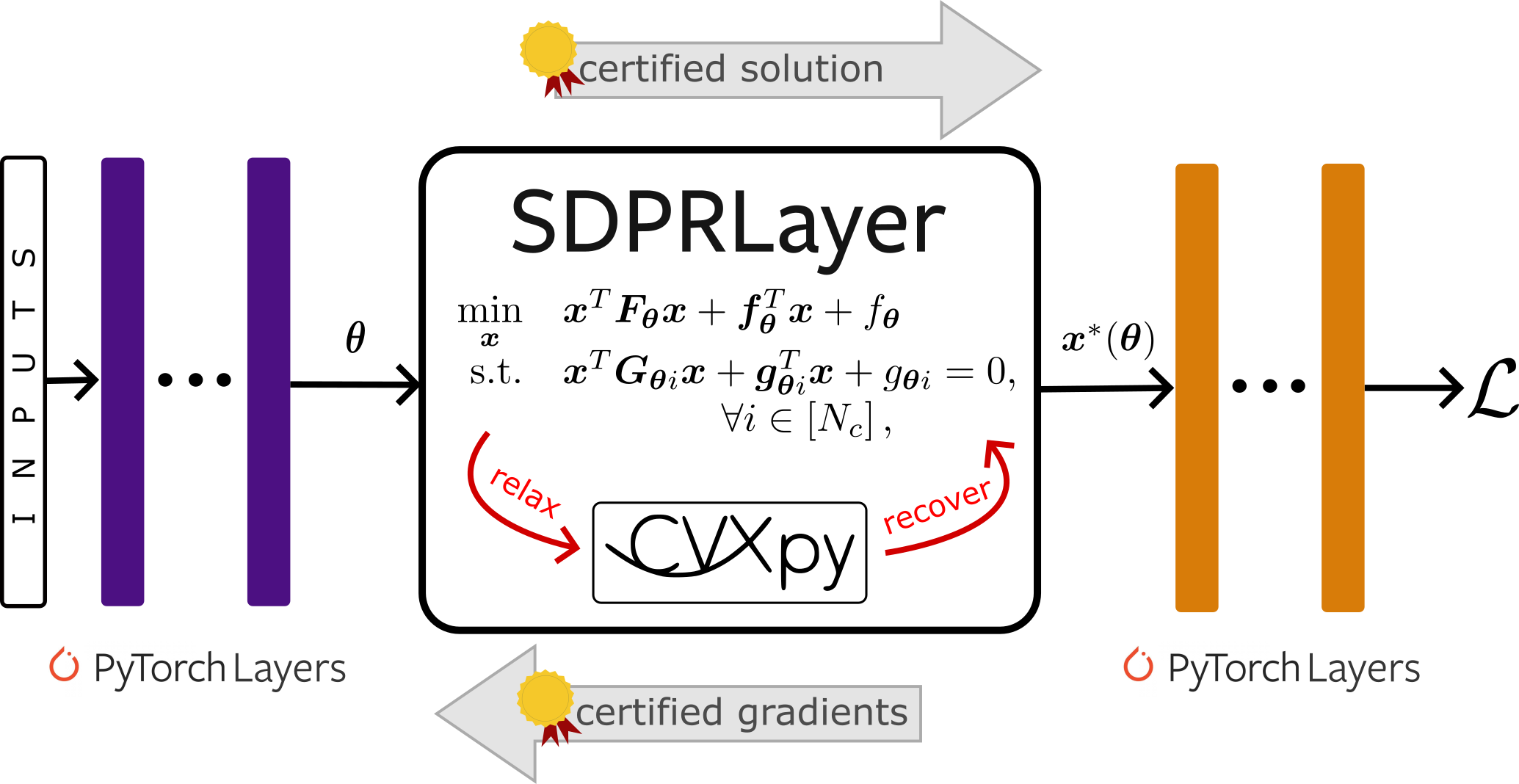
Figure 1: Our SDPRLayer embedded in a PyTorch autodifferentiation graph. For non-convex problems with tight semidefinite relaxations, the SDPRLayer finds the certified, globally optimal and differentiable solution by leveraging existing differentiable convex optimization layers. Existing differentiable solvers for non-convex problems can return incorrect gradients when they converge to local minima, which can corrupt the learning process. In contrast, the gradients produced by the SDPRLayer are always certified to be correct.

Many roboticists have adopted differentiable optimization layers into their pipelines. Building off their seminal work in differentiating quadratic programs (QPs) [4], Amos et al. [5] presented a differentiable Model Predictive Control (MPC) framework that enabled learning of dynamics and objective functions. This work was subsequently extended to integrate Reinforcement Learning (RL) and safe learning into MPC [55, 75, 23]. In robot planning, several works have developed differentiable approaches to dynamic programming [39, 19, 41]. Differentiable optimization has been used in physics-based simulators to enable efficient training of RL control strategies [15] or robotic hardware design [71]. In state estimation, DROID-SLAM, which introduced a differentiable, end-to-end, neural architecture for visual Simultaneous Localization and Mapping (SLAM) [63], is most notable, though there have been several works on differentiable SLAM [40, 27]. Differentiable optimization has also been used for factor-graph-based estimators [53] and smoothers [74], tactile sensing [61], and shape estimation [25].

Despite all of its success, there is a fundamental issue with differentiable optimization that has gone unaddressed in the literature; the majority of optimization problems addressed in robotics are non-convex and hence prone to convergence to local optima, rather than the global optimum. In this paper, we will highlight the potential issues that can arise if optimization layers are used naively. In particular, we demonstrate that if the optimization layer does not converge to the global optimum, the gradients that are backpropagated through the network will be completely incorrect, corrupting the training/optimization process. This can have serious consequences, leading not only to longer training times, but also outright failure to meet objectives of the training process.

We address this issue by leveraging a recent body of work in the robotics and vision communities that deals with so-called certifiably correct methods [58]. These methods use convex semidefinite relaxations of non-convex, polynomial optimization problems (POPs) to either directly find a global optimum or provide a certificate of global optimality for a given solution. In robotics, this approach has been applied to robust state estimation [72, 73], sensor calibration [70, 28], inverse kinematics [28], image segmentation [37], rotation averaging [16, 24], pose-graph optimization [57], multiple-point-set registration [12, 38], range-only localization [22, 30], and range-aided SLAM [51], among others. It is also worth noting that a similar approach using Sums-of-Squares (SOS) polynomials has been applied in the non-linear control community for automatic synthesis or verification of Lyapunov functions [47, 42].

In this paper, we focus on providing differentiable, globally optimal solutions to POPs. Although there is a variety of differentiable solvers that can find and differentiate first-order critical points for this class of problems, the resulting derivatives are correct only if the critical point is the global optimum. Moreover, certifying global optimality of a given solution to a POP is, in general, as computationally intensive as solving the semidefinite relaxation directly.

In contrast, our approach is to directly solve the semidefinite relaxations to obtain globally optimal solutions, then differentiate these solutions via existing, state-of-the-art techniques for implicit differentiation of convex optimization problems [1, 2]. We provide this approach as an optimization layer that conveniently encapsulates the convex reformulation and solver, which we call the SDPRLayer. As long as the POP admits a tight relaxation, the layer yields certifiably correct, differentiable solutions. It can be easily embedded in end-to-end learning or tuning pipelines for robotics problems, which we demonstrate in our experiments.

The most closely related work to ours is SATNet, introduced by Wang et al. [68], which uses semidefinite relaxations to generate approximate, differentiable solutions to the maximum satisfiability problem in combinatorial optimization. Amos et al. [5] also take a similar approach, applying a convex quadratic approximation to a non-convex MPC problem. On the other hand, our approach is a general framework directed at providing exact, differentiable solutions to robotics problems. Talak et al. [62] also makes use of certifiably correct methods, but does so only to verify correctness of solutions prior to backpropagation.

In Section II, we review relevant background material on implicit differentiation and semidefinite programming that may not be common knowledge to all readers, but that can be safely skipped by domain experts. Section  III provides a theoretical result that underpins our methodology. Section IV describes our methodology, including the implementation details of the SDPRLayer and modifications we have made to the existing differentiable, convex solver. In Section V, we provide two examples that demonstrate the advantages of our approach and a third that demonstrates its application to a real-world robotics problem. Finally, in Section VI, we present our conclusions, highlight the limitations of the current approach and provide ideas for future directions.

II Background

II-A Notation

We denote matrices with bold-faced, capitalized letters, $\bm{A}$, column vectors with bold-faced, lower-case letters, $\bm{a}$, and scalar quantities with normal-faced font, $a$. Let $\mathbb{S}^{n}$ denote the space of $n$-dimensional symmetric matrices, $\mathbb{S}_{+}^{n}$ denote the space of $n$-dimensional symmetric positive semidefinite matrices, and $\mathbb{S}_{1}^{n}\subset\mathbb{S}_{+}^{n}$ denote the set of positive, semidefinite, rank-1 matrices. We also use the conic notation $\bm{X}\succeq\bm{0}$ in place of $\bm{X}\in\mathbb{S}_{+}^{n}$. Let $\bm{I}$ denote the identity matrix, whose dimension will be clear from the context or otherwise specified. Let $\bm{0}$ denote the matrix with all-zero entries, whose dimension will be evident from the context. Let $\left[N\right]=\left\{1,\ldots,N\right\}\subset\mathbb{N}$ be the set of indexing integers. Let $\left<\bm{A},\bm{B}\right>=\mbox{tr}(\bm{A}^{T}\bm{B})$ denote the Frobenius inner product of matrices $\bm{A}$ and $\bm{B}$. Let $\|\cdot\|_{F}$ denote the Frobenius norm. Let $\mbox{SO}(d)$ denote the $d$-dimensional special orthogonal group.

II-B Implicit Differentiation

Implicit differentiation has become a key element of differentiable optimization, which applies the implicit function theorem to the set of conditions that characterize the optimum [20, 8]. The main idea is that the level set of the residual functions that represent these conditions defines an implicit function that uniquely links the optimization problem parameters to the solution. In general, this relationship is differentiable, providing a means to differentiate through optimization problems. Prior differentiation methods, such as unrolling, are either less accurate [8], slower, or more memory intensive than implicit differentiation [52].

When the problem is non-convex, implicit differentiation can be applied to any local optimum satisfying the (second-order) Karush-Kuhn-Tucker (KKT) conditions [31, 26]. Crucially, if the optimization layer converges to a local (rather than global) optimum, then the resulting implicit differentiation is incorrect for the true optimum.

On the other hand, when the problem is convex, implicit differentiation becomes much more powerful since the KKT conditions are sufficient and necessary for global optimality [9]. As such, it is often applied to convex problems or convex approximations of non-convex problems [4, 15, 68].

Agrawal et al. [1] introduced CVXPYLayers, a general differentiable solver for convex problems by interfacing the popular CVXPY parser [18] with a differentiable conic optimization solver [2]. This library has become the de-facto standard for differentiating convex programs and is a critical component of our implementation.

II-C Semidefinite Relaxations of Polynomial Optimization Problems

Many key problems in robotics can be expressed as polynomial optimization problems (POPs). In this section, we review the well-known procedure for deriving convex, SDP relaxations of a standard form of POP. This procedure was pioneered by Shor [59] and has become the cornerstone of certifiably correct methods in robotics and computer vision [58, 10].

We consider POPs that are parameterized on a variable, $\bm{\theta}\in\mathbb{R}^{m}$, and are formulated in the standard quadratically constrained quadratic problem (QCQP) form,

$$\begin{array}[]{rl}\min\limits_{\bm{x}}&\bm{x}^{T}\bm{F}_{\bm{\theta}}\bm{x}+\bm{f}_{\bm{\theta}}^{T}\bm{x}+f_{\bm{\theta}}\\ \mbox{s.t.}&\bm{x}^{T}\bm{G}_{\bm{\theta}i}\bm{x}+\bm{g}_{\bm{\theta}i}^{T}\bm{x}+g_{\bm{\theta}i}=0,\forall i\in\left[N_{c}\right],\end{array}$$ (1)

where $\bm{x}\in\mathbb{R}^{p}$ is the optimization variable, $\bm{F}_{\bm{\theta}}\in\mathbb{R}^{p\times p}$, $\bm{f}_{\bm{\theta}}\in\mathbb{R}^{p}$ and $f_{\bm{\theta}}\in\mathbb{R}$ represent the quadratic cost, and $\bm{G}_{\bm{\theta}i}\in\mathbb{R}^{p\times p}$, $\bm{g}_{\bm{\theta}i}\in\mathbb{R}^{p}$ and $g_{\bm{\theta}i}\in\mathbb{R}$ correspond to $N_{c}$ quadratic constraints. Note that any problem with polynomial objective and polynomial equality constraints can be expressed in the form of Problem (1). It is well known that this problem can be re-expressed in a standard homogenized form,

$$\begin{array}[]{rl}\min\limits_{\bm{x}}&\bm{x}^{T}\bm{Q}_{\bm{\theta}}\bm{x}\\ \mbox{s.t.}&\bm{x}^{T}\bm{A}_{\bm{\theta}i}\bm{x}=0,\forall i\in\left[N_{c}\right],\\ &\bm{x}^{T}\bm{A}_{0}\bm{x}=1,\end{array}$$ (2)

where the homogenizing constraint, $\bm{x}^{T}\bm{A}_{0}\bm{x}=1$, has been introduced to ensure that the optimization variable is homogeneous (i.e., $x_{i}=1$, for some $i\in 1,\dots,n$) and $\bm{x}\in\mathbb{R}^{n}$, where $n=p+1$. The exact form of the matrices, $\bm{Q}_{\bm{\theta}}$ and $\bm{A}_{\bm{\theta}i}$, and an explanation of this transformation can be found in [14] or [29]. Problem (2) can then be re-expressed in terms of semidefinite matrices by using the properties of the trace operator as follows:

$$\begin{array}[]{rl}\min\limits_{\bm{X}}&\left<\bm{Q}_{\bm{\theta}},\bm{X}\right>\\ s.t.&\left<\bm{A}_{\bm{\theta}i},\bm{X}\right>=0,\quad\forall i\in\left[N_{c}\right]\\ &\left<\bm{A}_{0},\bm{X}\right>=1,\\ &\bm{X}\succeq\bm{0},\\ &\mbox{rank}(\bm{X})=1,\end{array}$$ (3)

where the last two constraints implicitly enforce the fact that $\bm{X}=\bm{x}\bm{x}^{T}$.

II-C1 Relaxing the QCQP

In general, problems with quadratic equality constraints, such as QCQPs, are difficult to solve optimally because they are non-convex [9]. In Problem (3), we see that all the non-convexity of the problem has been relegated to a single non-convex constraint on the rank. It follows that we can find a convex relaxation of Problem (3) by removing the rank constraint:

$$\begin{array}[]{rl}\min\limits_{\bm{X}}&\left<\bm{Q}_{\bm{\theta}},\bm{X}\right>\\ s.t.&\left<\bm{A}_{\bm{\theta}i},\bm{X}\right>=0,\quad\forall i\in\left[N_{c}\right]\\ &\left<\bm{A}_{0},\bm{X}\right>=1,\\ &\bm{X}\succeq\bm{0}.\\ \end{array}$$ (4)

This relaxation – known as Shor’s relaxation – has been well studied by the optimization community and can also be derived via Lagrangian duality of Problem (2) (c.f. [34]).

II-C2 Recovering the Global Solution

When the optimal solution of Problem (4), $\bm{X}^{*}$, satisfies $\mbox{rank}\left(\bm{X}^{*}\right)=1$ then the convex relaxation is said to be tight to the original QCQP and the SDP solution can be factorized as $\bm{X}^{*}=\bm{x}^{*}\bm{x}^{*T}$ to obtain the globally optimal solution, $\bm{x}^{*}$, of Problem (1). This result has been proved rigorously by Cifuentes et al. [14], among others, and depends on the inherent properties of the QCQP formulation and the fact that strong duality holds generically for SDPs. The stability of the ‘tightness’ of semidefinite relaxations under perturbations to the objectives and constraints of the original QCQP was also studied extensively by Cifuentes et al. [14]. We leverage these stability results in Section IV to prove our main theorem.

In what follows, we will make use of a recovery map, $\mathcal{R}:\mathbb{S}_{1}^{n}\rightarrow\mathbb{R}^{n}$. Given a solution, $\bm{X}^{*}$, to Problem (4) that is rank-1, we apply this map to recover a solution to Problem (1), $\bm{x}^{*}=\mathcal{R}(\bm{X}^{*})$.

Since the problem is homogenized, $\bm{x}^{*}$ can be extracted directly from the $i^{th}$ column of $\bm{X}^{*}$ (with the $i^{th}$ row removed), where $i$ corresponds to the index of the homogenization variable. Clearly this mapping is both smooth and differentiable since it only involves projection.

II-C3 Adding Redundant Constraints

For some problems in robotics and vision, the SDP relaxation is not immediately tight, but can be made so by adding so-called redundant constraints to the original QCQP [21, 35, 10, 73, 72]. Although redundant in the original QCQP, these constraints are not redundant for the SDP relaxation.

A recent work has also shown how these redundant constraints can be efficiently and automatically generated for use in different state estimation problems that do not initially have tight relaxations [21].

More generally, it has been shown that, subject to a mild technical condition [49], any POP (including those problems that we have cited) can be tightened via a standard semidefinite relaxation hierarchy introduced by Lasserre [44] (referred to as Lasserre’s moment hierarchy). Yang and Carlone [72] provide a thorough-yet-accessible introduction to these ideas for robotics practitioners.

II-C4 Solving SDPs Efficiently

In general, SDPs can be solved in polynomial time using interior-point methods [66]. These methods are fast for small problems and even tractable for problems of up to thousands of variables, but become prohibitive when real-time deployment is desired. Since this paper is mostly concerned with offline tuning and training, realtime operation is not a key concern of this paper. However, we acknowledge that efficient SDP solvers are important for the application of our approach. Majumdar et al. [47] and Rosen [56] provide excellent overviews of methods that can be used to improve runtime of SDP solvers for robotics applications.

II-D Directional Derivatives and Jacobians

We briefly review some key concepts in this section that will be useful for our theoretical results in the next section. Let $\bm{x}:\mathbb{R}^{m}\rightarrow\mathbb{R}^{n}$ be a differentiable vector function. The directional derivative of $\bm{x}$ at a point $\bm{\theta}\in\mathbb{R}^{m}$ along a unit-length direction vector $\bm{v}\in\mathbb{R}^{m}$ is given by

$$\mathrm{D}\bm{x}(\bm{\theta})\left[\bm{v}\right]=\lim\limits_{t\rightarrow 0}\frac{\bm{x}(\bm{\theta}+t\bm{v})-\bm{x}(\bm{\theta})}{t},$$ (5)

where $t\in\mathbb{R}$. The Jacobian of $\bm{x}$ evaluated at $\bm{\theta}$, $\mathrm{D}\bm{x}(\bm{\theta})$, can be found by plugging in the canonical basis vectors, $\bm{e}_{j}$ and $\bm{e}_{i}$, for the input and output spaces of $\bm{x}$, respectively, so that

$$\mathrm{D}\bm{x}(\bm{\theta})\in\mathbb{R}^{n\times m},\quad\left[\mathrm{D}\bm{x}(\bm{\theta})\right]_{ij}=\left<\bm{e}_{i},\mathrm{D}\bm{x}(\bm{\theta})\left[\bm{e}_{j}\right]\right>.$$ (6)

II-E The Solution Map and Its Jacobian

In this paper, we adopt the approach of Barratt [7], Agrawal et al. [3, 2] and view an optimization problem as a mapping between a set of input parameters, $\bm{\theta}$, and a set of solutions to the optimization. We refer to this mapping as a solution map. We are chiefly concerned with the solution map of the QCQP, Problem (1), which we denote by $\bm{x}^{*}(\bm{\theta})$, but will also make use of the solution map of the SDP relaxation, Problem (4), which we denote by $\bm{X}^{*}(\bm{\theta})$.

In the context of bilevel optimization frameworks [43], the solution map becomes the ‘inner’ optimization, which must be solved (often multiple times) in order to minimize some outer loss function, $\mathcal{L}$,

$$\min\limits_{\bm{\theta}}\mathcal{L}(\bm{x}^{*}(\bm{\theta})).$$ (7)

In the context of neural network training, this inner optimization represents a differentiable optimization layer. The preceding layers of the network provide the parameters $\bm{\theta}$ to the layer, which then solves the inner optimization in the forward pass. In the backward pass, the Jacobian of $\bm{x}^{*}(\bm{\theta})$ is computed and used to backpropagate gradients through the network.

In either case, a key challenge is to compute the Jacobian of the solution map, denoted by $\mathrm{D}\bm{x}^{*}(\bm{\theta})$, which can then be used for autodifferentiation. In theory, Problem (1) can be solved using any non-linear, non-convex optimization solver and its solution map can be differentiated by applying the implicit function theorem to the (second-order) KKT conditions, as shown by various authors [26, 8, 54].

However, in practice, there is a serious issue with this approach; there is no guarantee that the non-linear solver will converge to the global optimum of Problem (1). Indeed, if the solver converges to a local optimum, then subsequent differentiation will occur with respect to the local solution instead of the true solution. By contrast, our approach always obtains the globally optimal solution and therefore always returns correct gradients, as long as the upfront work of finding a tight relaxation to the POP has been completed.

III Theory

In this section, we present a theorem that, under certain technical conditions, shows how to compute the exact Jacobian of $\bm{x}^{*}(\bm{\theta})$. The key insight of the theorem is that this Jacobian can be obtained from the solution map of the convex relaxation, $\bm{X}^{*}(\bm{\theta})$, as long as the relaxation is tight at the solution. In turn, the Jacobian of $\bm{X}^{*}(\bm{\theta})$ is found by implicit differentiation of its KKT conditions, using CVXPYLayers [1].

Theorem 1 (QCQP Jacobian).

For a given set of parameter values, $\bm{\theta}$, let $\bm{X}^{*}(\bm{\theta})$ be the rank-1 solution to the SDP (4). Let $\bm{x}^{*}(\bm{\theta})$ be the solution to the QCQP (1) and let the pair $(\bm{x}^{*}(\bm{\theta}),\bm{\theta})$ satisfy the conditions of [14, Theorem 4.2]. That is, the Abadie constraint qualifications hold at $\bm{x}^{*}(\bm{\theta})$, and the mapping from $\bm{\theta}$ to the feasible set of the QCQP (1) is smooth near $(\bm{x}^{*}(\bm{\theta}),\bm{\theta})$. Further, let the $\bm{A}_{i}(\bm{\theta})$ matrices be linearly independent. Then,

$$\mathrm{D}\bm{x}^{*}(\bm{\theta})=\mathrm{D}\mathcal{R}(\bm{X}^{*}(\bm{\theta}))~{}\mathrm{D}\bm{X}^{*}(\bm{\theta}).$$ (8)

Moreover, there exists a perturbation, $d\bm{\theta}$, such that the QCQP with the perturbed parameter, $\bm{\theta}^{\prime}=\bm{\theta}+d\bm{\theta}$, also has a rank-1 relaxation and, to first order, the globally optimal solution of the perturbed problem satisfies $\bm{x}^{*}(\bm{\theta}^{\prime})=\bm{x}^{*}(\bm{\theta})+\mathrm{D}\bm{x}^{*}(\bm{\theta})d\bm{\theta}$.

Proof:

Consider the directional derivative of $\bm{x}^{*}(\bm{\theta})$:

$$\mathrm{D}\bm{x}^{*}(\bm{\theta})\left[\bm{v}\right]=\lim\limits_{t\rightarrow 0}\frac{\bm{x}^{*}(\bm{\theta}+t\bm{v})-\bm{x}^{*}(\bm{\theta})}{t}.$$

Since $\bm{X}^{*}(\bm{\theta})$ is rank-1 by assumption, it follows that $\bm{x}^{*}(\bm{\theta})=\mathcal{R}(\bm{X}^{*}(\bm{\theta}))$. Moreover, [14, Theorem 4.2] implies that $\bm{X}^{*}(\bm{\theta}+d\bm{\theta})$ is also rank-1 for sufficiently small $d\bm{\theta}$. In our case, $d\bm{\theta}=t\bm{v}$ is a small perturbation in the limit, so we have that the optimal solution to the perturbed problem is exactly given by $\bm{x}^{*}(\bm{\theta}+t\bm{v})=\mathcal{R}(\bm{X}^{*}(\bm{\theta}+t\bm{v}))$. By the definition of the directional derivative, we have

$$\mathrm{D}\bm{x}^{*}(\bm{\theta})\left[\bm{v}\right] =\lim\limits_{t\rightarrow 0}\frac{\bm{x}^{*}(\bm{\theta}+t\bm{v})-\bm{x}^{*}(\bm{\theta})}{t}$$

$$=\lim\limits_{t\rightarrow 0}\frac{\mathcal{R}(\bm{X}^{*}(\bm{\theta}+t\bm{v}))-\mathcal{R}(\bm{X}^{*}(\bm{\theta}))}{t}.$$ (9)

We note that $\mathcal{R}$ is trivially differentiable, since it is a linear projection. Conditions for differentiability of solutions of non-linear programs in general are provided by Fiacco and Ishizuka [26, Theorem 5.1]. These conditions are satisfied for Problem (4), since, by assumption of linear independence of the constraint matrices, $\bm{A}_{i}$, the linear independence constraint qualification (LICQ) holds. Therefore, we also have that $\bm{X}^{*}(\bm{\theta})$ is differentiable with Jacobian $\mathrm{D}\bm{X}^{*}(\bm{\theta})$.

From the differentiability of these two maps, it follows that

$$\mathcal{R}(\bm{X}^{*}(\bm{\theta}+t\bm{v}))-\mathcal{R}(\bm{X}^{*}(\bm{\theta}))\\ =\mathrm{D}\mathcal{R}(\bm{X}^{*}(\bm{\theta}))~{}\mathrm{D}\bm{X}^{*}(\bm{\theta})~{}t\bm{v}+\bm{o}(t),$$

where $\bm{o}(\cdot)$ denotes Landau (‘little-o’) notation. Therefore, in the limit, we have

$$\mathrm{D}\bm{x}^{*}(\bm{\theta})\left[\bm{v}\right]=\mathrm{D}\mathcal{R}(\bm{X}^{*}(\bm{\theta}))~{}\mathrm{D}\bm{X}^{*}(\bm{\theta})~{}t\bm{v}.$$

Evaluating the directional derivative at canonical vectors, we find the exact Jacobian of $\bm{x}^{*}(\bm{\theta})$ is given by

$$\mathrm{D}\bm{x}^{*}(\bm{\theta})=\mathrm{D}\mathcal{R}(\bm{X}^{*}(\bm{\theta}))~{}\mathrm{D}\bm{X}^{*}(\bm{\theta}),$$

as desired. The final statement of the theorem follows directly from the development above, with $d\bm{\theta}=t\bm{v}$. ∎

Remark 1 (Theorem 1 in Practice).

A key implication of this theorem is that the parameters, $\bm{\theta}$, can be ‘tuned’ according to gradients computed using $\mathrm{D}\bm{x}^{*}(\bm{\theta})$ without losing the rank-1 property of the SDP relaxation. This means that global optimality guarantees will hold throughout the tuning process (e.g., during neural network training). While it is theoretically possible that taking a parameter step that is too large may result in loss of this tightness property, we have not observed this phenomenon in our experimentation.

Remark 2 (Satisfaction of Conditions).

The constraint qualification and feasible set smoothness conditions of Theorem 1 are typical in many optimization problems and are used to ensure the existence of Lagrange multipliers. The rank-1 condition is more restrictive, but is satisfied by many of the certifiable optimization problems studied by the robotics and vision communities. As mentioned in Section II, the rank-1 condition can be attained in some problems by adding redundant constraints and, more generally, for any POP using Lasserre’s hierarchy. Finally, the assumption of linear independence of the $\bm{A}_{\bm{\theta}i}$ matrices does not preclude the use of redundant constraints discussed in Section II and is generally good practice for computational stability when solving the SDP.

IV Methodology and Implementation

In this section, we introduce our implementation, the SDPRLayer, which computes the differentiable, globally optimal solution to a polynomial optimization problem and can be embedded in any PyTorch autodifferentiation graph. A key prerequisite to the application of our method is that the initial parameterization of the POP must have a tight SDP relaxation. Since it is crucial to our methodology, a procedure for finding tight relaxations of a given POP is provided in Appendix -A.

An outline of the architecture of the SDPRLayer is presented in Section IV-A and our specific modifications to its (existing) underlying solver are given in Section IV-B.

IV-A SDPRLayer Architecture

As one of our contributions, we provide an encapsulation of our method in a PyTorch neural network module. This module is effectively a convenient wrapper around (a modified version of) CVXPYLayers [1] that has been specialized for QCQPs and their relaxations. We have chosen to use CVXPYLayers because its interface is straightforward, it has a PyTorch implementation, and is the only differentiable solvers that natively supports SDPs, to the authors’ knowledge.

The expected input for our layer is a set of Pytorch tensors representing the problem, either in standard form, Problem (1), or in the equivalent homogenized form, Problem (2), depending on the preference of the user. The output of our layer is a PyTorch tensor representing the differentiable solution map, $\bm{x}^{*}(\bm{\theta})$, which can be used in succeeding layers of the PyTorch compute graph.

In the forward pass, our optimization layer performs three key steps:

1. Formulate SDP: In the case that the user has provided the QCQP in non-homogeneous form, the SDPRLayer first homogenizes the problem via a standard approach (see Cifuentes et al. [14] for details). The resulting data and constraint matrices, $(\bm{Q}_{\bm{\theta}},\left\{\bm{A}_{\bm{\theta}i}\right\})$, are then used to set up the SDP relaxation, Problem (4), as a disciplined convex program (DCP) using the CVXPYLayers interface. The problem can be formulated in primal or dual form based on the preference of the user.

2. Solve SDP: The DCP is then solved by (our version of) CVXPYLayers, which returns the differentiable solution map, $\bm{X}^{*}(\bm{\theta})$. On backpropagation, CVXPYLayers propagates the gradients of this solution map using implicit differentiation of the KKT conditions evaluated at the solution point. Additional arguments can be passed to the SDPRLayer to select the internal solver and solver arguments that are used by CVXPYLayers to solve the DCP.

3. Recover Rank-1 Solution: The recovery map is then used to recover the globally optimal solution of the POP from the solution of the DCP, $\bm{x}^{*}(\bm{\theta})=\mathcal{R}(\bm{X}^{*}(\bm{\theta}))$. As mentioned above, this is accomplished by selecting the column of $\bm{X}^{*}(\bm{\theta})$ corresponding to the homogenizing variable, a linear operation.

All of these steps are implemented in PyTorch, making backpropagation straightforward for the user. For the convenience of the user, we have also added a method to the SDPRLayer module that directly assesses the tightness of the SDP solution. This function computes the ratio of the maximum two eigenvalues of the SDP solution,

$$r=\frac{\lambda_{1}(\bm{X}^{*}(\bm{\theta}))}{\lambda_{2}(\bm{X}^{*}(\bm{\theta}))},$$

where, for $\bm{A}\in\mathbb{R}^{n}$, $\lambda_{i}(\bm{A})$ denotes the $i^{th}$ eigenvalue of $\bm{A}$, where $\lambda_{1}\geq\dots\geq\lambda_{n}$. If the ratio exceeds a given threshold then the solution can be considered to be rank-1, and the relaxation is tight. Empirically, we have found a ratio of $r=1\times 10^{6}$ to be a good indicator of relaxation tightness.

IV-B Modifications to CVXPYLayers

The canonicalization used by CVXPY can often lead to inefficiencies when converting a DCP to a cone program. We have observed this empirically for the SDPs studied in robotics, depending on the solver to be used. This issue can be avoided by formulating the problem in dual form, but the implementation of CVXPYLayers did not previously support differentiation of slack or dual variables. As such, we have modified the interface of CVXPYLayers (and its underlying dependencies) to expose the (differentiable) Lagrange multipliers and slack variables as outputs, since they are already computed by the underlying solvers.

We also extended the interface to allow external SDP solvers to be used, as long as they provide the requisite primal, dual, and slack solution variables. In this case, the forward pass simply injects the solution variables from the external solver, bypassing the optimization. On the backward pass, the stored variables are used by the existing implicit differentiation machinery. We have tested this approach extensively and used it to solve problems with Mosek [6], which is often faster and more robust than SCS [50], the default solver used by CVXPYLayers.

V Experiments

We now present a series of examples that demonstrate the utility of our method in comparison to (non-global) alternatives. The first two experiments are simulated and highlight the potential issues with naive application of differentiable optimization. The final experiment shows how our approach can be used to train a deep neural net in a real-world robotics pipeline. Note that the preceding theory allows both cost and constraints to be functions of parameters, but our examples focus on cases where the constraints are fixed.

V-A Polynomial Experiment

In this section, we consider a bilevel polynomial optimization problem that clearly illustrates the potential issues that can arise when local optimization is used to find $\bm{x}^{*}(\bm{\theta})$. The objective of this problem is to find a sixth-order polynomial that has a global minimum at a pre-specified point, $(\bar{x},\bar{y})$. The polynomial function is parameterized by its coefficients $\bm{\theta}$,

$$y(x,\bm{\theta})=\sum_{i=0}^{6}\theta_{i}x^{i}.$$ (10)

The task is split into an inner optimization, which attempts to find the global minimum of the current polynomial, and an outer optimization, which tunes the polynomial coefficients to shift the minimum to the specified point. The bilevel optimization can be written as follows:

$$\begin{array}[]{rl}\min\limits_{\bm{\theta}}&(x^{*}(\bm{\theta})-\bar{x})^{2}+(y(x^{*}(\bm{\theta}),\bm{\theta})-\bar{y})^{2}\\ s.t.&x^{*}(\bm{\theta})=\mbox{arg}\min\limits_{x}y(x,\bm{\theta}).\end{array}$$ (11)

Though this example does not have direct application in robotics, it is a simplified analogue of robotics problems in reinforcement learning, where an overparameterized value function must be learned to achieve a specific task.

V-A1 Problem Parameters

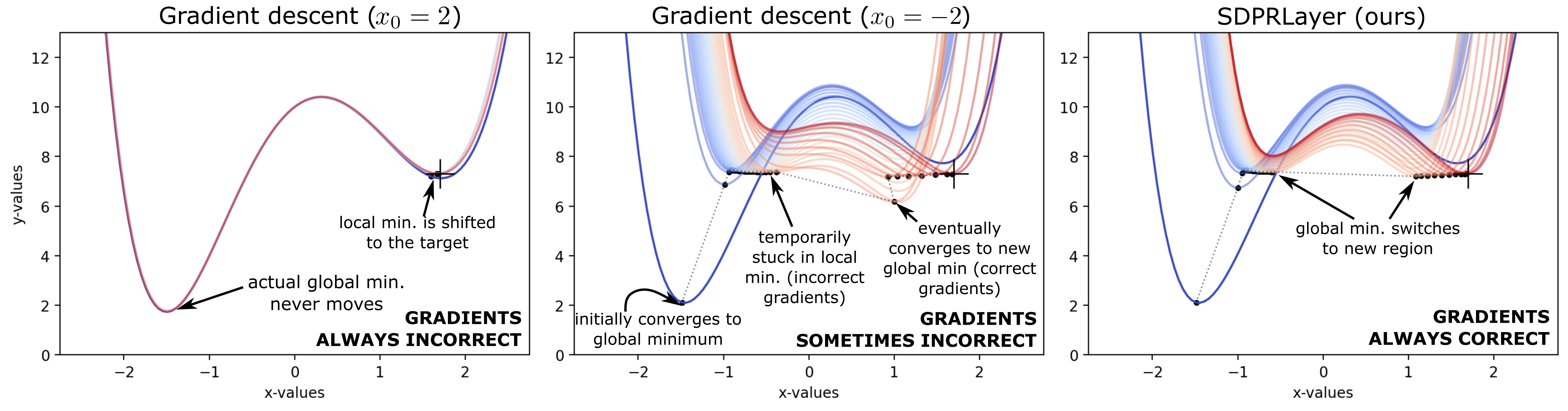
Figure 2: Evolution of the polynomial function throughout the bilevel optimization. Columns present different methods for solving the inner optimization problem: (left) gradient descent initialized at $x=2$, (centre) gradient descent initialized at $x=-2$, and (right) our approach. In all three cases, the color of the function indicates the progress of outer loop iterations (blue at the beginning, red at the end), the black dots indicate the minima found by the inner optimization, and the plus sign indicates the target. All three cases converge, but gradient descent only converges to a valid solution when it is initialized well ($x_{0}=-2$) and, even then, is temporarily trapped in a local minimum. SPDRLayer converges to a valid solution, does not require initialization, and is even able to discontinuously ‘switch’ the minimum to a new region.

In this example, the target global minimum is $(\bar{x},\bar{y})=(1.7,7.3)$ and we initialized the polynomial coefficients as shown in Table I.

TABLE I: Initial Polynomial Coefficients

$\theta_{0}$	$\theta_{1}$	$\theta_{2}$	$\theta_{3}$	$\theta_{4}$	$\theta_{5}$	$\theta_{6}$
10.0	2.6334	-4.3443	0.0	0.8055	-0.1334	0.0389

V-A2 Inner Optimization

We consider two different methods for solving the inner optimization. The first method is a standard non-linear gradient descent (GD) method, implemented in PyTorch. On the first outer iteration, this method requires an initialization point, $x_{0}$, but subsequent (inner) optimizations are initialized using the previous minimum. Since we are dealing with a polynomial, $\mathrm{D}\bm{x}^{*}(\bm{\theta})$ can be computed analytically using the implicit function theorem (c.f. [31]).

The second method is a tight SDP relaxation of the inner optimization, which is implemented using the SDPRLayer. The parameterized cost matrix is given by

$$\bm{Q}_{\bm{\theta}}=\begin{bmatrix}\theta_{0}&\frac{1}{2}\theta_{1}&\frac{1}{3}\theta_{2}&\frac{1}{4}\theta_{3}\\ \frac{1}{2}\theta_{1}&\frac{1}{3}\theta_{2}&\frac{1}{4}\theta_{3}&\frac{1}{3}\theta_{4}\\ \frac{1}{3}\theta_{2}&\frac{1}{4}\theta_{3}&\frac{1}{3}\theta_{4}&\frac{1}{2}\theta_{5}\\ \frac{1}{4}\theta_{3}&\frac{1}{3}\theta_{4}&\frac{1}{2}\theta_{5}&\theta_{6}\\ \end{bmatrix}.$$

The following constraints lead to a tight semidefinite relaxation:

$$\bm{A}_{1}=\begin{bmatrix}0&0&\frac{1}{2}&0\\ 0&-1&0&0\\ \frac{1}{2}&0&0&0\\ 0&0&0&0\\ \end{bmatrix},\quad\bm{A}_{2}=\begin{bmatrix}0&0&0&1\\ 0&0&-1&0\\ 0&-1&0&0\\ 1&0&0&0\\ \end{bmatrix},$$

$$\bm{A}_{3}=\begin{bmatrix}0&0&0&0\\ 0&0&0&\frac{1}{2}\\ 0&0&-1&0\\ 0&\frac{1}{2}&0&0\\ \end{bmatrix}.$$

Note that, for this example, the constraints are not a function of the parameter $\bm{\theta}$.

V-A3 Outer Optimization

Since the outer optimization is unconstrained, we find the minimum using gradient descent, with the gradients being computed based on the solution map of the inner optimization. The optimization is terminated when the loss function has a value less than $1\times 10^{-4}$.

V-A4 Results

The progression of the bilevel optimization is shown in Figure 2. The key observation is that when gradient descent is used, the convergence of the overall optimization to a valid solution depends heavily on the initialization point.

When gradient descent is initialized at $x_{0}=2$ (left plot), the solution converges to and remains at a local minimum of the polynomial. The gradients that are computed here correspond to the local minimum solution, thus the outer optimization then shifts the local minimum of the polynomial to the target point, while the global minimum remains largely unchanged.

When gradient descent is initialized at $x_{0}=-2$ (centre plot), the solution initially converges to the global minimum and provides valid gradients. As the outer iterations proceed, the inner optimization temporarily gets stuck in a local minimum. At this point, the outer optimization pushes the new global minimum in the wrong direction until the inner optimization eventually converges to the new global minimum. Subsequently, gradient descent is able to reach a valid solution, though it did so in 13% more iterations than SDPRLayer. This last case shows that initializing the inner optimization well does not guarantee that it will not get stuck in a local minimum at some point during the optimization, hence providing incorrect gradient information.

In stark contrast to gradient descent, the SPDRLayer always converges to the global solution of the problem and therefore always provides the correct gradients to the outer optimization (right plot). As a consequence, the outer optimization is able to consistently push the global minimum towards the target, and is even able to switch discontinuously to a different minimum as necessary.

V-B Stereo Baseline Calibration Example

In this example, we calibrate the stereo baseline of a camera rig via camera localization. We once again adopt a bilevel optimization strategy in which the inner optimization uses the stereo measurements to solve a camera localization problem and the outer optimization fine-tunes the stereo baseline to minimize an overall loss function.

It is assumed that we have stereo camera measurements of a known set of $N_{m}$ features, that the data association is known, and that there are no outliers. Pixel measurements are converted into Euclidean measurements using the following inverse, differentiable, stereo-camera model (see Gridseth and Barfoot [33, Section IIIC] for details):

$$\bm{m}_{k}=\frac{b}{d_{k}}\begin{bmatrix}u_{k}-c_{u}\\ \frac{f_{u}}{f_{v}}(v_{k}-c_{v})\\ f_{u}\end{bmatrix},$$ (12)

where $\bm{m}_{k}\in\mathbb{R}^{3}$ is the Euclidean measurement of the $k^{th}$ feature, $b$ is the camera baseline, $f_{u}$ and $f_{v}$ are the horizontal and vertical focal lengths for the cameras, respectively, and $c_{u}$ and $c_{v}$ are the horizontal and vertical centres for the cameras, respectively. The left-camera horizontal, vertical, and disparity measurements (in pixels) of the $k^{th}$ feature are given by $u_{k}$, $v_{k}$, and $d_{k}$, respectively.

The (pixel-space) measurements are assumed to be perturbed by Gaussian noise with standard deviations of $\sigma_{u}$ and $\sigma_{v}$ in the horizontal and vertical directions, respectively. In turn, the Euclidean measurements are also perturbed by noise,

$$\tilde{\bm{m}}_{k}=\bm{m}_{k}+\bm{\epsilon}_{k},$$ (13)

where $\bm{\epsilon}_{k}$ is a zero-mean Gaussian noise term with covariance matrix $\bm{W}^{-1}_{k}$. This matrix is a function of the camera parameters and can be computed as shown in shown in [35].

The maximum-likelihood camera pose can be found by solving the matrix-weighted localization problem [35]:

$$\begin{array}[]{rl}\min\limits_{\bm{C},\bm{t}}&\sum\limits_{k=1}^{N_{m}}\bm{e}_{k}^{T}\bm{W}_{k}(\bm{\theta})\bm{e}_{k}\\ \mbox{s.t.}&\bm{C}\in\mbox{SO}(3),\\ &\bm{e}_{k}=\tilde{\bm{m}}_{k}(\bm{\theta})-\bm{C}(\bm{m}_{k}+\bm{t}),\end{array}$$ (14)

where $\bm{\theta}$ represents the camera baseline, $\bm{C}$ and $\bm{t}$ are the camera pose rotation and translation, $\bm{m}_{k}$ is a feature point with known location, $\tilde{\bm{m}}_{k}(\bm{\theta})$ is the Euclidean measurement of the point from the camera frame and $\bm{W}_{k}(\bm{\theta})$ is its associated inverse-covariance, matrix weight.

Problem (14) constitutes the inner optimization. The loss minimized by the outer optimization is the squared error between estimated camera pose and ground-truth camera pose,

$$\begin{array}[]{rl}\min\limits_{\bm{\theta}}&\|\bm{t}^{*}(\bm{\theta})-\bm{t}_{gt}\|_{2}^{2}+\|\bm{C}^{*}(\bm{\theta})^{T}\bm{C}_{gt}-\bm{I}\|_{F}^{2}\end{array},$$ (15)

where $\left\{\bm{C}^{*}(\bm{\theta}),\bm{t}^{*}(\bm{\theta})\right\}$ is the estimated pose from the inner optimization and $\left\{\bm{C}_{gt},\bm{t}_{gt}\right\}$ represents the ground-truth pose. We note that this loss is not necessarily feasible in practice since ground-truth data are not always available. However, in our context, this simplified loss makes comparison between approaches more straightforward.

Since the outer optimization is unconstrained it can be solved iteratively using stochastic gradient descent.

V-B1 Problem Parameters

We ran simulated experiments using the stereo camera parameters given in Table II. The features, $\bm{m}_{k}$, were arranged in an equally spaced grid occupying a 1.0 m by 1.0 m rectangle located at the origin (similar to a checkerboard). In each experiment, 20 camera poses were placed randomly at a radius of 3 m from the centre of the grid, within a 90 degree cone. Orientations of the camera poses were also randomized, but it was ensured that the centre of the grid points were within a 90 degree field of view of the camera. Figure 3a provides a diagram of the setup for an example pose.

TABLE II: Ground-Truth Camera Parameters

Parameter	$b$	$f_{u}$	$f_{v}$	$c_{u}$	$c_{v}$	$\sigma_{u}$	$\sigma_{v}$
Units	m	$\frac{\mbox{pix}}{\mbox{m}}$	$\frac{\mbox{pix}}{\mbox{m}}$	pix	pix	pix	pix
Values	0.24	484.5	484.5	0.0	0.0	0.5	0.5

V-B2 Solving the Inner Optimization

Since Problem (14) is a non-linear least-squares problem, with $\mbox{SO}(3)$ Lie group constraints, it can be solved using the Theseus optimization framework [52]. Moreover, as shown by Holmes et al. [35], Problem (14) also has a tight semidefinite relaxation.

We implemented both Theseus and the SDPRLayer to solve the inner optimization and provide a comparison of the results. In the Theseus implementation, we use a Gauss-Newton solver with a stepsize of $0.2$ and relative error tolerance of $1\times 10^{-6}$, and select ‘IMPLICIT’ as the backpropagation mode.

Since Theseus is a local solver, it requires an initial estimate of the pose to solve Problem (14). Similar to the polynomial example, after the first iteration, the inner optimization is warm-started with the previous solution. We investigated situations in which Theseus is initialized with both the ground-truth and randomized initializations in order to demonstrate the effect of convergence to local minima. The random initializations used in this context are exemplified in Figure 3b; translations are randomly selected on the surface of a 3 m ball around the feature grid (at the origin), with orientation selected such that the $z$-axis points at the centre of the grid and the other two axes are random. Figure 3b shows that roughly 60% the initializations converge to poor local minima.

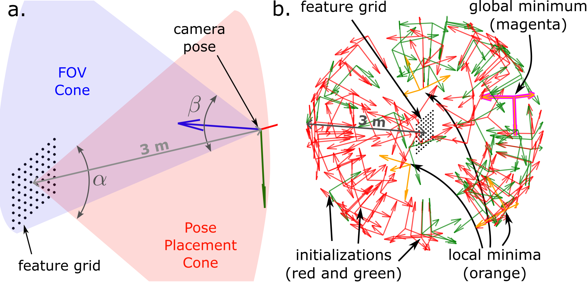
Figure 3: a. Setup for one of the ground-truth poses used in the stereo tuning example. The position of the ground-truth poses are placed 3 m from the centre of the grid in a cone of angle $\beta=90~{}\mbox{deg}$ (red cone). The poses are oriented such that the centre of the grid is within the field of view (FOV) of the camera ($z$) axis, $\alpha=90~{}\mbox{deg}$. b. 100 random initialization samples for Theseus’ Gauss-Newton solver. The initializations are color coded based on whether they converged to the local minimum (red) or global minimum (green). The local and global solutions are orange and magenta frames, respectively.

In contrast, the SDPRLayer does not require any initialization and always finds the globally optimal solution. The backend of the SDPRLayer implementation used the Splitting Conic Solver (SCS) to solve the SDP with tolerance set to $1\times 10^{-9}$ [50].

V-B3 Results

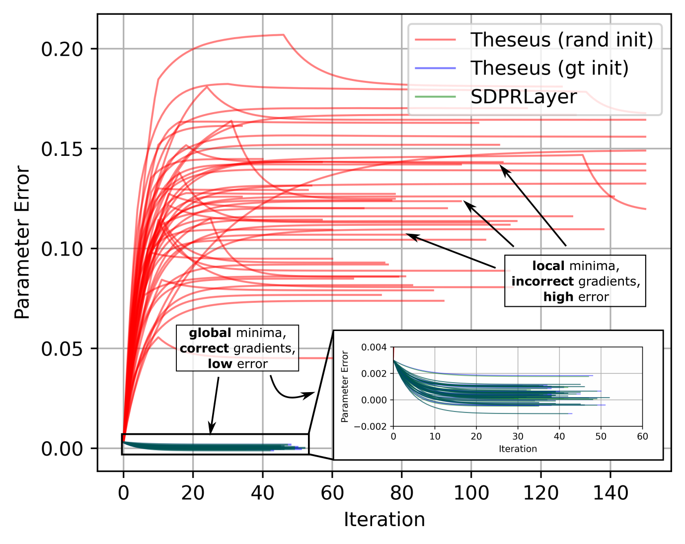
Figure 4: Baseline parameter error trajectories across outer optimization iterations for 50 trials with different inner loop optimization approaches. Theseus with ground-truth initialization and SDPRLayer always converge to global minima, hence provide correct gradients to the outer opt. Theseus with random initialization sometimes converges to local minima and therefore provides incorrect gradients to the outer optimization, resulting in large parameter error.

We ran 50 stereo calibration experiments with different ground-truth poses and compared the results between Theseus – with ground-truth and random initializations – and our approach. In all three cases, the outer optimization (baseline calibration) was identical. The baseline parameter was initialized with a 0.003 m error from the true value and the outer optimization was solved using stochastic gradient descent with a learning rate of $1\times 10^{-4}$. Each experiment terminated when the outer optimization gradient magnitude was less than $1\times 10^{-3}$ or 150 iterations had been reached. We stress that the only difference in the Theseus approaches shown in this section is the initialization used.

The parameter error trajectories for the different approaches are shown in Figure 4 across outer optimization iterations and aggregate results are provided in Table III. From Figure 4, it is clear that initializing randomly causes convergence to camera baseline values that are completely incorrect. By contrast, both our approach and Theseus with ground-truth initialization converge to a low level of error in a shorter number of iterations. Note that the individual trajectories of these two approaches are very close to each other. This is confirmed by the investigation of the gradients and inner optimization error in Figure 5. This is to be expected, since both approaches converge to the global minimum and thus return almost exactly the same gradients (subject to numerical precision of solvers).

TABLE III: Baseline Tuning Results Across Runs

Method	Final Baseline Error (avg)	Final Baseline Error (std)	Number of Outer Iterations (avg)	Outer Loss (avg)
Theseus (rand init)	1.210e-01	2.991e-02	9.728e+01	1.426e+02
Theseus (gt init)	3.797e-04	5.241e-04	4.018e+01	1.020e-02
SDPRLayer (ours)	3.727e-04	5.226e-04	3.992e+01	1.020e-02

Our investigations suggest that the divergence of the randomly initialized Theseus approach is exactly because the inner optimization converges to local minima for some poses. In turn, this leads to gradients that push the baseline in the wrong direction. Evidence of poor gradient information can also be observed in Figure 5. Initial experimentation suggests that the ‘kinks’ in the red trajectories of Figure 4 occur because some poses of the batch are able to escape local minima and converge to the true solution as the baseline parameter changes.

The aggregate results in Table III corroborate our findings in Figure 4; random initialization leads to poor tuning overall, increasing the number of required iterations, the average error and variation of tuned parameter. Again, our approach and Theseus with ground-truth initialization match very closely.

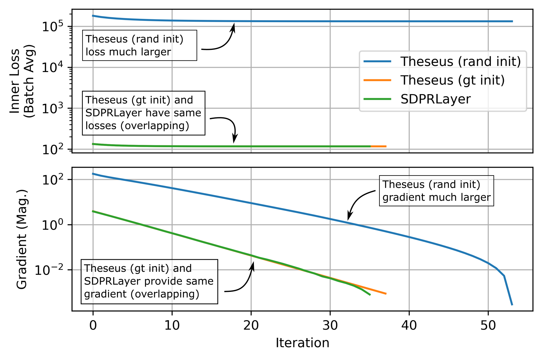
Figure 5: Inner optimization losses and gradient information for one of the experiments. It is clear that SDPRLayer and Theseus with ground-truth initialization match very well, while randomly initializing Theseus leads to incorrect gradient values. The large (average) inner optimization loss for Theseus (rand init) is a clear indicator of the presence of local minima.

V-C Deep Learned Visual Features for Localization

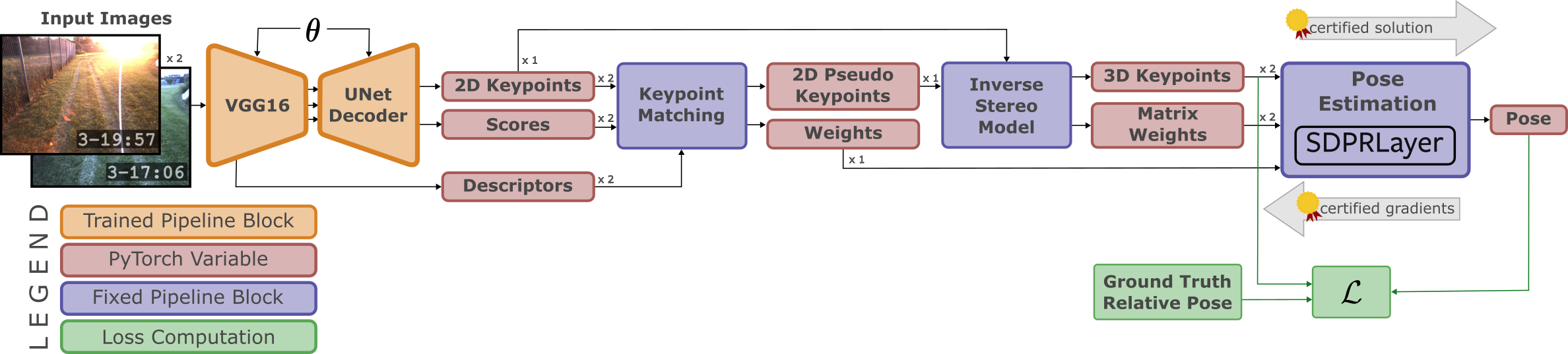
Figure 6: Diagram of our Pytorch pipeline (based on the pipeline in [33]) that we use to estimate the relative pose between two images (i.e., localize a target image to a (stored) source image). Orange blocks denote the deep neural networks whose weights are tuned during training (VGG16 network and UNet Decoder network). Blue blocks denote blocks that are part of the pipeline, but do not have trainable parameters. Red blocks indicate key PyTorch tensor variables. Green blocks and arrows indicate training loss function computation.

In this section, we show that our approach can extend to large, real-world robotics problems. We consider the task of supervised learning of visual features for robot localization when environment lighting conditions can change drastically. Note that our goal here is not to match the state of the art, but to demonstrate that the SDPRLayer can be used to train deep neural networks for robotics applications. In particular, we adopt the learning pipeline introduced by Gridseth and Barfoot [33] for stereo-vision-based robot localization.

Our adaptation of this fully differentiable pipeline is shown in Figure 6. A convolutional neural network is used to extract keypoints along with descriptors and scores for an RGB, stereo-image pair (four images total). The keypoints for the left source and target image are matched, converted to 3D coordinates (using a stereo camera model and disparity), and used to compute a relative pose with a differentiable pose estimator. The scores and descriptor match determine the relative (scalar) weighting of the keypoint pairs in the estimation (see (5) in [33]).

The final stage of the original pipeline used a Singular Value Decomposition (SVD) to compute the relative pose between the images, since it provides a closed-form and differentiable solution (see Umeyama [65] for the details). However, since this method only supports scalar weights in the cost function, it cannot fully incorporate the (directional) uncertainty of keypoints that are derived from stereo images. Accounting for this uncertainty properly has been shown to be important for accurate state estimation in robotics [48, 69, 46].

To properly account for the measurement uncertainty, we replace the pose-estimation block of the baseline pipeline with the matrix-weighted pose optimization, Problem (14), implemented using the SDPRLayer with Mosek as the internal solver. The matrix weights are computed based on the inverse covariance of each 3D keypoint, which is known based on camera model and assumed pixel-space covariance. The matrix weights are then scaled by the scalar weights provided by the matching block in the pipeline.

Similar to Chen and Barfoot [13], we replace the encoder segment of the neural network with a VGG16 network (truncated at conv_5_3 layer) [60] that has been pretrained on ImageNet [17] to facilitate faster training. The remainder of the pipeline was not changed.

V-C1 Training

We kept as many parameters unchanged as possible between the baseline training setup and our setup. The feature detector network was trained for 35 epochs (10000 samples in each epoch) on an NVIDIA Tesla V100 DGXS GPU using the same keypoint and pose estimation training loss as in [33] (see (7) and (8) therein). The same weightings between the losses were used and the pose-estimation loss was ignored for a ‘warm-up’ period of 10 epochs.

For training, we used 100000 training samples and 20000 validation samples from the ‘In-The-Dark’ dataset, which was also used for training by Gridseth and Barfoot [33] and has many instances of severe lighting changes. Using the Adam optimizer with a learning rate of $1\times 10^{-4}$, the decoder network was trained from scratch and the VGG16 network was fine-tuned from its pretrained weights.

V-C2 Testing

We compare our pipeline (‘Ours’) against the baseline pipeline (‘Baseline’) used in [33] on a set of test runs that were held out of the training and validation data. In particular, we tested the localization pipelines on all souce-target stereo-image pairs from all combinations of runs 2, 11, 16, 17, 23, 28, and 35 from the In-The-Dark dataset and assessed the error based on comparison with ground truth. Test runs for the baseline were performed using the available code and network weight parameters associated with [33].

It is assumed that ground truth data is unavailable during inference. As such, a random sample consensus (RANSAC) was used in the matching block to find the correct set of inliers. The pose estimation within the RANSAC algorithm was consistent with the pose estimation used in each pipeline (Ours: SDPRLayer, Baseline: SVD).

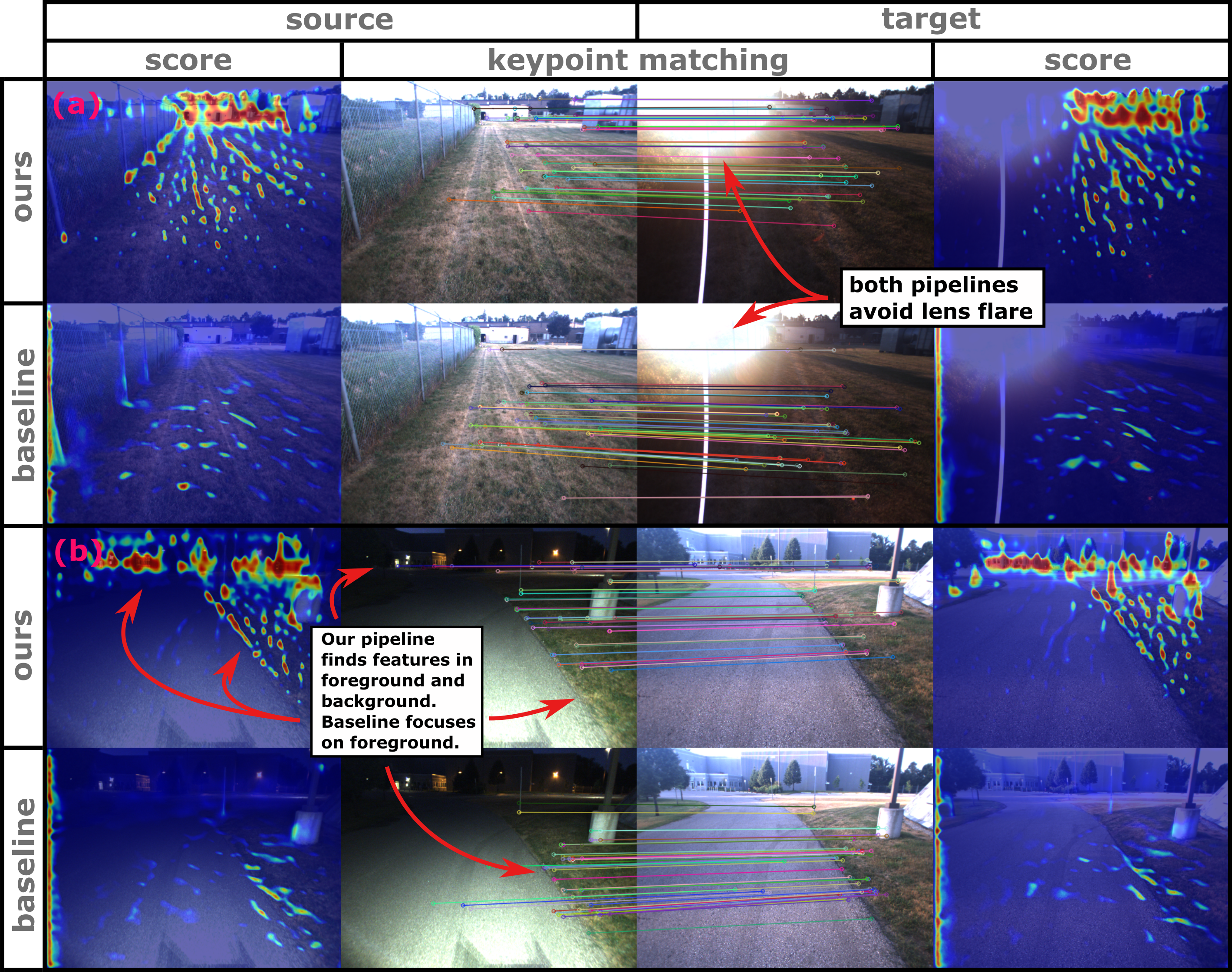
Figure 7: Scores and keypoint matches for two selected stereo-image pairs from the In-The-Dark dataset. No outlier filtering has taken place at this stage in the pipeline. Image pair (a) corresponds to source (Run 27, Frame 2182) and target (Run 8, Frame 1886) and demonstrates ‘lens flare’. Image pair (b) corresponds to source (Run 21, Frame 2057) and target (Run 27, Frame 1830) and demonstrates a night-day match. The keypoint-match images (centre two columns) display the source and target images with the 50 highest-weighted keypoint matches overlaid. The score columns show the score map from the neural network corresponding to their adjacent images.

V-C3 Results

Table IV shows number of inliers (from RANSAC), longitudinal position error, lateral position error,16 heading (yaw) error,16 and inference time per pose, averaged across all runs. A full set of results for all runs is provided in Appendix -B. Although we score consistently worse than the baseline on average, we note that the inlier rate and errors are not significantly different from the baseline and are small enough to be used in a robotics pipeline. Since the SDP used to globally solve Problem (14) is relatively small, the average inference time with the SDPRLayer was only three times longer than inference with the original SVD pose estimation. We also point out that the baseline pipeline has been trained for approximately 17 times more epochs than our pipeline and on a significantly larger dataset (included ‘multiseason’ data)[32].

TABLE IV: Summary of Average Inliers and Localization Error Across Test Runs

Pipe-
line	Avg.
Inliers	Long.
Pos.
Err. (m)	Lat.
Pos.
Err. (m)	Head.
Err.
(deg)	Avg. Inf.
Time
(s)	# train.
epochs
Base-
line	542.48	0.025	0.013	0.245	0.081	585
Ours	542.29	0.024	0.013	0.247	0.211	30

The qualitative performance of each pipeline is assessed in Figure 7, which provides the scores and keypoint matches on two samples from the In-the-Dark dataset. Both pipelines successfully find a good set of keypoint matches and manage to avoid problems induced by drastic lighting changes (i.e., ‘lens flare’ and night-day matching).

We note that the baseline consistently focuses on keypoints in the foreground. We speculate that this is because, during training, the network cannot separate the high depth uncertainty from the low lateral uncertainty in faraway measurements and is forced to downweight the background keypoints.

On the other hand, our pipeline characterizes this directional uncertainty using the matrix weights. It is therefore able to distribute the keypoints more heavily in the background of the images than the baseline. We note in passing that this can be quite advantageous in localization because keypoints that are farther away typically provide better information about orientation, while close features give better information about translation.

The experiment shown in this section clearly shows that our SDPRLayer can be used to train neural networks in real-world robotics pipelines.

VI Conclusion and Future Work

We have presented the SDPRLayer, a differentiable optimization layer for polynomial optimization problems with tight semidefinite relaxations. We have demonstrated that differentiable optimization approaches with local solvers often return completely incorrect gradients during backpropagation due to convergence to local minima. By extension, the outer training/optimization process may be lengthened or even fail entirely to achieve its objective. On the other hand, we provided theoretical and experimental results showing that the SDPRLayer provides certified gradients, in the sense that they correspond to the certified, global minimum of the optimization problem.

The examples shown in this paper have demonstrated the potential pitfalls of naive application of differentiable optimization. The last example demonstrates that the SDPRLayer can be used for real-world robotics applications that combine deep-learned and model-based components.

To initially demonstrate our approach, we have relied on CVXPYLayers. Though it is an effective general convex optimization solver, CVXPYLayers is not specialized to our specific problem, which inherently leads to inefficiencies. Another serious limitation of CVXPYLayers is that the forward step (optimization) must take place on the CPU, leading to costly memory transfers when training with a GPU.

Tailoring the solver and implicit differentiation of the convex relaxation to the explicit problem formulation can allow us to exploit sparsity, leverage the properties of SDPs, and optimize in parallel, directly on a GPU. These are necessary future steps to the application of SDPRLayers and, more generally, certifiable methods to larger robotics problems.

Finally, we believe that SDPRLayers could be applied to other areas of robotics apart from the perception methods demonstrated in this paper. In particular, differentiable Model Predictive Control is an exciting problem that has been recently studied in the literature [55] and may benefit from certifiable gradients in practice.

-A Finding a Tight Relaxation

The following procedure can be used to find tight relaxations to POPs:

1. A given POP of some variable, $\bm{z}\in\mathbb{R}^{p}$, can always be reformulated as Problem (1) (or, alternatively, Problem (2)) using the approach outlined in Carlone [11] or Yang and Carlone [72]. Roughly speaking, this involves selecting a set of monomials of $\bm{z}$ that are capable of representing the problem in QCQP form. These monomials are collected in a new variable $\bm{x}$, and constraints are added to enforce the relationship between $\bm{x}$ and $\bm{z}$.

2. Once formulated as a QCQP, the relaxed Problem (4) can be solved and the rank of the solution can be tested. The solution and the rank test can be performed using our SDPRLayers module.

3. If the relaxation is not tight, then the iterative procedure outlined by Dümbgen et al. [21] can be used to find a tight relaxation:

   1. This procedure first finds all possible redundant constraints for the QCQP. These constraints are gradually added until the relaxation becomes tight.

   2. If all constraints have been added and the relaxation is still not tight, then additional variables can be added to $\bm{x}$ by increasing the degree of the monomials used in the formulation. The procedure then continues from Step 2.

Figure 8 provides a visual representation of this procedure. There are some guarantees on when this procedure – or more generally, Lasserre’s hierarchy – results in a tight relaxation [45], but it can also lead to intractably large SDPs. Finding efficient, tight relaxations for POPs remains an active area of research.

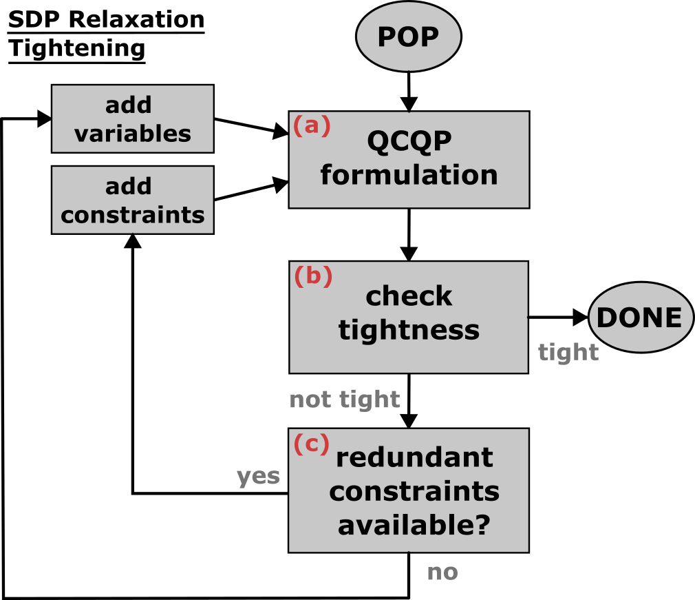
Figure 8: General algorithm for tightening an SDP relaxation of a POP. Given a POP, (a) a QCQP can be formulated using the methods discussed in [72] or [11]. (b) Tightness of the relaxation can be assessed using the SDPRLayer presented herein (Section -A). (c) If the relaxation is not tight, [21] provides a method to discover all possible constraints which can be added to improve tightness. If the relaxation is still not tight, then variables can be added (i.e., move to a higher level of Lasserre’s hierarchy).

-B Test Run Results for Deep Learned Stereo Localization

The table below provides the aggregate results from each of the test runs used to assess the pipelines in Section V-C.

[ caption=Localization and Inlier and Error Results Across Test Runs ]rllrrrr Src.
Run Targ.
Run Pipe-
line Avg.
Inliers Long.
Pos.
Err.
(m) Lat.
Pos.
Err.
(m) Head.
Err.
(deg)
2 11 Baseline 584 0.023 0.009 0.130
2 11 Ours 582 0.016 0.007 0.105
2 16 Baseline 524 0.039 0.017 0.306
2 16 Ours 518 0.028 0.017 0.321
2 17 Baseline 520 0.039 0.018 0.337
2 17 Ours 515 0.031 0.019 0.372
2 23 Baseline 585 0.025 0.009 0.140
2 23 Ours 581 0.019 0.009 0.125
2 28 Baseline 555 0.025 0.012 0.235
2 28 Ours 552 0.020 0.011 0.223
2 35 Baseline 593 0.021 0.009 0.147
2 35 Ours 593 0.021 0.009 0.125
11 16 Baseline 527 0.027 0.016 0.303
11 16 Ours 523 0.021 0.016 0.320
11 17 Baseline 523 0.027 0.018 0.348
11 17 Ours 520 0.023 0.017 0.371
11 23 Baseline 587 0.017 0.008 0.148
11 23 Ours 588 0.013 0.007 0.150
11 28 Baseline 557 0.021 0.011 0.241
11 28 Ours 555 0.019 0.010 0.258
11 35 Baseline 587 0.021 0.009 0.184
11 35 Ours 584 0.016 0.008 0.176
16 17 Baseline 516 0.021 0.016 0.316
16 17 Ours 522 0.016 0.015 0.299
16 23 Baseline 512 0.020 0.014 0.255
16 23 Ours 519 0.019 0.015 0.258
16 28 Baseline 492 0.030 0.016 0.306
16 28 Ours 493 0.059 0.020 0.306
16 35 Baseline 514 0.027 0.015 0.269
16 35 Ours 519 0.025 0.013 0.260
17 23 Baseline 509 0.021 0.014 0.270
17 23 Ours 516 0.022 0.015 0.293
17 28 Baseline 489 0.031 0.017 0.337
17 28 Ours 491 0.042 0.019 0.339
17 35 Baseline 512 0.029 0.015 0.280
17 35 Ours 516 0.027 0.013 0.290
23 28 Baseline 560 0.021 0.012 0.264
23 28 Ours 558 0.016 0.011 0.252
23 35 Baseline 581 0.024 0.009 0.147
23 35 Ours 581 0.016 0.007 0.122
28 35 Baseline 565 0.024 0.011 0.185
28 35 Ours 562 0.037 0.014 0.231

References

- Agrawal et al. [2019a] Akshay Agrawal, Brandon Amos, Shane Barratt, Stephen Boyd, Steven Diamond, and J. Zico Kolter. Differentiable Convex Optimization Layers. In Advances in Neural Information Processing Systems, volume 32. Curran Associates, Inc., 2019a.
- Agrawal et al. [2019b] Akshay Agrawal, Shane Barratt, Stephen Boyd, Enzo Busseti, and Walaa Moursi. Differentiating Through A Cone Program. J. Appl. Numer. Optim, 1(2):107–115, 2019b.
- Agrawal et al. [2021] Akshay Agrawal, Shane Barratt, and Stephen Boyd. Learning Convex Optimization Models. IEEE/CAA Journal of Automatica Sinica, 8(8):1355–1364, August 2021.
- Amos and Kolter [2021] Brandon Amos and J. Zico Kolter. OptNet: Differentiable Optimization as a Layer in Neural Networks. arXiv:1703.00443, December 2021.
- Amos et al. [2018] Brandon Amos, Ivan Jimenez, Jacob Sacks, Byron Boots, and J. Zico Kolter. Differentiable MPC for End-to-end Planning and Control. In Advances in Neural Information Processing Systems, volume 31. Curran Associates, Inc., 2018.
- ApS [2024] MOSEK ApS. MOSEK Optimizer API for Python, March 2024.
- Barratt [2021] Shane Thomas Barratt. Convex Optimization and Implicit Differentiation Methods for Control and Estimation. PhD thesis, Stanford University, United States – California, 2021.
- Blondel et al. [2022] Mathieu Blondel, Quentin Berthet, Marco Cuturi, Roy Frostig, Stephan Hoyer, Felipe Llinares-Lopez, Fabian Pedregosa, and Jean-Philippe Vert. Efficient and Modular Implicit Differentiation. Advances in Neural Information Processing Systems, 35:5230–5242, December 2022.
- Boyd and Vandenberghe [2004] Stephen P. Boyd and Lieven Vandenberghe. Convex Optimization. Cambridge University Press, Cambridge, UK ; New York, 2004.
- Brynte et al. [2022] Lucas Brynte, Viktor Larsson, José Pedro Iglesias, Carl Olsson, and Fredrik Kahl. On the Tightness of Semidefinite Relaxations for Rotation Estimation. Journal of Mathematical Imaging and Vision, 64(1):57–67, January 2022.
- Carlone [2023] Luca Carlone. Estimation Contracts for Outlier-Robust Geometric Perception. Foundations and Trends® in Robotics, 11(2-3):90–224, June 2023.
- Chaudhury et al. [2015] K. N. Chaudhury, Y. Khoo, and A. Singer. Global Registration of Multiple Point Clouds Using Semidefinite Programming. SIAM Journal on Optimization, 25(1):468–501, January 2015.
- Chen and Barfoot [2023] Yuxuan Chen and Timothy D. Barfoot. Self-Supervised Feature Learning for Long-Term Metric Visual Localization. IEEE Robotics and Automation Letters, 8(2):472–479, February 2023.
- Cifuentes et al. [2022] Diego Cifuentes, Sameer Agarwal, Pablo A. Parrilo, and Rekha R. Thomas. On the local stability of semidefinite relaxations. Mathematical Programming, 193(2):629–663, June 2022.
- de Avila Belbute-Peres et al. [2018] Filipe de Avila Belbute-Peres, Kevin Smith, Kelsey Allen, Josh Tenenbaum, and J. Zico Kolter. End-to-End Differentiable Physics for Learning and Control. In Advances in Neural Information Processing Systems, volume 31. Curran Associates, Inc., 2018.
- Dellaert et al. [2020] Frank Dellaert, David M. Rosen, Jing Wu, Robert Mahony, and Luca Carlone. Shonan Rotation Averaging: Global Optimality by Surfing . In Andrea Vedaldi, Horst Bischof, Thomas Brox, and Jan-Michael Frahm, editors, Computer Vision – ECCV 2020, volume 12351, pages 292–308. Springer International Publishing, Cham, 2020.
- Deng et al. [2009] Jia Deng, Wei Dong, Richard Socher, Li-Jia Li, Kai Li, and Li Fei-Fei. ImageNet: A large-scale hierarchical image database. In 2009 IEEE Conference on Computer Vision and Pattern Recognition, pages 248–255, June 2009.
- [18] Steven Diamond and Stephen Boyd. CVXPY: A Python-Embedded Modeling Language for Convex Optimization.
- Dinev et al. [2022] Traiko Dinev, Carlos Mastalli, Vladimir Ivan, Steve Tonneau, and Sethu Vijayakumar. Differentiable Optimal Control via Differential Dynamic Programming. arXiv:2209.01117, September 2022.
- Dontchev and Rockafellar [2014] Asen L. Dontchev and R. Tyrrell Rockafellar. Implicit Functions and Solution Mappings: A View from Variational Analysis. Springer Series in Operations Research and Financial Engineering. Springer New York, New York, NY, 2014.
- Dümbgen et al. [2023a] Frederike Dümbgen, Connor Holmes, Ben Agro, and Timothy D. Barfoot. Toward Globally Optimal State Estimation Using Automatically Tightened Semidefinite Relaxations. arXiv:2308.05783, August 2023a.
- Dümbgen et al. [2023b] Frederike Dümbgen, Connor Holmes, and Timothy D. Barfoot. Safe and Smooth: Certified Continuous-Time Range-Only Localization. IEEE Robotics and Automation Letters, 8(2):1117–1124, February 2023b.
- East et al. [2020] S. East, M. Gallieri, J. Masci, J. Koutnik, and M. Cannon. Infinite-horizon differentiable Model Predictive Control. Proceedings of ICLR 2020, 2020.
- Eriksson et al. [2018] Anders Eriksson, Carl Olsson, Fredrik Kahl, and Tat-Jun Chin. Rotation Averaging and Strong Duality. In 2018 IEEE/CVF Conference on Computer Vision and Pattern Recognition, pages 127–135, Salt Lake City, UT, June 2018. IEEE.
- Fan et al. [2021] Taosha Fan, Kalyan Vasudev Alwala, Donglai Xiang, Weipeng Xu, Todd Murphey, and Mustafa Mukadam. Revitalizing Optimization for 3D Human Pose and Shape Estimation: A Sparse Constrained Formulation. In 2021 IEEE/CVF International Conference on Computer Vision (ICCV), pages 11437–11446, Montreal, QC, Canada, October 2021. IEEE.
- Fiacco and Ishizuka [1990] Anthony V. Fiacco and Yo Ishizuka. Sensitivity and stability analysis for nonlinear programming. Annals of Operations Research, 27(1):215–235, December 1990.
- Fu et al. [2023] Taimeng Fu, Shaoshu Su, and Chen Wang. iSLAM: Imperative SLAM. arXiv:2306.07894, July 2023.
- Giamou et al. [2022] Matthew Giamou, Filip Marić, David M. Rosen, Valentin Peretroukhin, Nicholas Roy, Ivan Petrović, and Jonathan Kelly. Convex Iteration for Distance-Geometric Inverse Kinematics. IEEE Robotics and Automation Letters, 7(2):1952–1959, April 2022.
- Giamou [2023] Matthew Peter Giamou. Semidefinite Relaxations for Geometric Problems in Robotics. Thesis, March 2023.
- Goudar et al. [2024] Abhishek Goudar, Frederike Dümbgen, Timothy D. Barfoot, and Angela P. Schoellig. Optimal Initialization Strategies for Range-Only Trajectory Estimation. IEEE Robotics and Automation Letters, 9(3):2160–2167, March 2024.
- Gould et al. [2016] Stephen Gould, Basura Fernando, Anoop Cherian, Peter Anderson, Rodrigo Santa Cruz, and Edison Guo. On Differentiating Parameterized Argmin and Argmax Problems with Application to Bi-level Optimization. arXiv:1607.05447, July 2016.
- Gridseth [2022] Mona Gridseth. Towards Deep Learning for Long-term Visual Localization in Visual Teach and Repeat. Thesis, November 2022.
- Gridseth and Barfoot [2022] Mona Gridseth and Timothy D. Barfoot. Keeping an Eye on Things: Deep Learned Features for Long-Term Visual Localization. IEEE Robotics and Automation Letters, 7(2):1016–1023, April 2022.
- Holmes and Barfoot [2023] Connor Holmes and Timothy D. Barfoot. An Efficient Global Optimality Certificate for Landmark-Based SLAM. IEEE Robotics and Automation Letters, 8(3):1539–1546, March 2023.
- Holmes et al. [2023] Connor Holmes, Frederike Dümbgen, and Timothy D. Barfoot. On Semidefinite Relaxations for Matrix-Weighted State-Estimation Problems in Robotics. arXiv:2308.07275, August 2023.
- Howell et al. [2023] Taylor A. Howell, Kevin Tracy, Simon Le Cleac’h, and Zachary Manchester. CALIPSO: A Differentiable Solver for Trajectory Optimization with Conic and Complementarity Constraints. In Aude Billard, Tamim Asfour, and Oussama Khatib, editors, Robotics Research, pages 504–521, Cham, 2023. Springer Nature Switzerland.
- Hu and Carlone [2019] Siyi Hu and Luca Carlone. Accelerated Inference in Markov Random Fields via Smooth Riemannian Optimization. IEEE Robotics and Automation Letters, 4(2):1295–1302, April 2019.
- Iglesias et al. [2020] Jose Pedro Iglesias, Carl Olsson, and Fredrik Kahl. Global Optimality for Point Set Registration Using Semidefinite Programming. In 2020 IEEE/CVF Conference on Computer Vision and Pattern Recognition (CVPR), pages 8284–8292, Seattle, WA, USA, June 2020. IEEE.
- Jallet et al. [2022] Wilson Jallet, Nicolas Mansard, and Justin Carpentier. Implicit Differential Dynamic Programming. In 2022 International Conference on Robotics and Automation (ICRA), pages 1455–1461, Philadelphia, PA, USA, May 2022. IEEE.
- Jatavallabhula et al. [2020] Krishna Murthy Jatavallabhula, Ganesh Iyer, and Liam Paull. SLAM: Dense SLAM meets Automatic Differentiation. In 2020 IEEE International Conference on Robotics and Automation (ICRA), pages 2130–2137, Paris, France, May 2020. IEEE.
- Jin et al. [2020] Wanxin Jin, Zhaoran Wang, Zhuoran Yang, and Shaoshuai Mou. Pontryagin Differentiable Programming: An End-to-End Learning and Control Framework. In Advances in Neural Information Processing Systems, volume 33, pages 7979–7992. Curran Associates, Inc., 2020.
- Kang et al. [2023] Shucheng Kang, Yuxiao Chen, Heng Yang, and Marco Pavone. Verification and Synthesis of Robust Control Barrier Functions: Multilevel Polynomial Optimization and Semidefinite Relaxation. arXiv:2303.10081, March 2023.
- Landry [2021] Benoit Landry. Differentiable and Bilevel Optimization for Control in Robotics. PhD thesis, Stanford University, United States – California, 2021.
- Lasserre [2001] Jean B. Lasserre. Global Optimization with Polynomials and the Problem of Moments. SIAM Journal on Optimization, 11(3):796–817, January 2001.
- Lasserre [2010] Jean-Bernard Lasserre. Moments, Positive Polynomials and Their Applications. Number v. 1 in Imperial College Press Optimization Series. Imperial College Press ; Distributed by World Scientific Publishing Co, London : Signapore ; Hackensack, NJ, 2010.
- Maimone et al. [2007] Mark Maimone, Yang Cheng, and Larry Matthies. Two years of Visual Odometry on the Mars Exploration Rovers. Journal of Field Robotics, 24(3):169–186, March 2007.
- Majumdar et al. [2020] Anirudha Majumdar, Georgina Hall, and Amir Ali Ahmadi. Recent Scalability Improvements for Semidefinite Programming with Applications in Machine Learning, Control, and Robotics. Annual Review of Control, Robotics, and Autonomous Systems, 3(1):331–360, 2020.
- Matthies and Shafer [1987] L Matthies and S A Shafer. Error Modeling in Stereo Navigation. IEEE Journal of Robotics and Automation, RA-3(3):12, June 1987.
- Nie [2014] Jiawang Nie. Optimality conditions and finite convergence of Lasserre’s hierarchy. Mathematical Programming, 146(1):97–121, August 2014.
- O’Donoghue et al. [2016] Brendan O’Donoghue, Eric Chu, Neal Parikh, and Stephen Boyd. Conic Optimization via Operator Splitting and Homogeneous Self-Dual Embedding. Journal of Optimization Theory and Applications, 169(3):1042–1068, June 2016.
- Papalia et al. [2023] Alan Papalia, Andrew Fishberg, Brendan W. O’Neill, Jonathan P. How, David M. Rosen, and John J. Leonard. Certifiably Correct Range-Aided SLAM. arXiv:2302.11614, February 2023.
- Pineda et al. [2022] Luis Pineda, Taosha Fan, Maurizio Monge, Shobha Venkataraman, Paloma Sodhi, Ricky Chen, Joseph Ortiz, Daniel DeTone, Austin Wang, Stuart Anderson, Jing Dong, Brandon Amos, and Mustafa Mukadam. Theseus: A Library for Differentiable Nonlinear Optimization. arXiv:2207.09442, July 2022.
- Qadri and Kaess [2023] Mohamad Qadri and Michael Kaess. Learning Observation Models with Incremental Non-Differentiable Graph Optimizers in the Loop for Robotics State Estimation. arXiv:2309.02525, September 2023.
- Robinson [1980] Stephen M. Robinson. Strongly Regular Generalized Equations. Mathematics of Operations Research, 5(1):43–62, 1980.
- Romero et al. [2023] Angel Romero, Yunlong Song, and Davide Scaramuzza. Actor-Critic Model Predictive Control. arXiv:2306.09852, September 2023.
- Rosen [2021] David M. Rosen. Scalable Low-Rank Semidefinite Programming for Certifiably Correct Machine Perception. In Steven M. LaValle, Ming Lin, Timo Ojala, Dylan Shell, and Jingjin Yu, editors, Algorithmic Foundations of Robotics XIV, volume 17, pages 551–566. Springer International Publishing, Cham, 2021.
- Rosen et al. [2019] David M Rosen, Luca Carlone, Afonso S Bandeira, and John J Leonard. SE-Sync: A certifiably correct algorithm for synchronization over the special Euclidean group. The International Journal of Robotics Research, 38(2-3):95–125, March 2019.
- Rosen et al. [2021] David M. Rosen, Kevin J. Doherty, Antonio Terán Espinoza, and John J. Leonard. Advances in Inference and Representation for Simultaneous Localization and Mapping. Annual Review of Control, Robotics, and Autonomous Systems, 4(1):215–242, 2021.
- Shor [1987] N.Z. Shor. Quadratic optimization problems. Soviet Journal of Computer and Systems Sciences, 25:1–11, 1987.
- Simonyan and Zisserman [2015] Karen Simonyan and Andrew Zisserman. Very Deep Convolutional Networks for Large-Scale Image Recognition. arXiv:1409.1556, April 2015.
- Sodhi et al. [2021] Paloma Sodhi, Michael Kaess, Mustafa Mukadam, and Stuart Anderson. Learning Tactile Models for Factor Graph-based Estimation. In 2021 IEEE International Conference on Robotics and Automation (ICRA), pages 13686–13692, Xi’an, China, May 2021. IEEE.
- Talak et al. [2023] Rajat Talak, Lisa R. Peng, and Luca Carlone. Certifiable Object Pose Estimation: Foundations, Learning Models, and Self-Training. IEEE Transactions on Robotics, 39(4):2805–2824, August 2023.
- [63] Zachary Teed and Jia Deng. DROID-SLAM: Deep Visual SLAM for Monocular, Stereo, and RGB-D Cameras.
- Teed and Deng [2021] Zachary Teed and Jia Deng. Tangent Space Backpropagation for 3D Transformation Groups. In 2021 IEEE/CVF Conference on Computer Vision and Pattern Recognition (CVPR), pages 10333–10342, Nashville, TN, USA, June 2021. IEEE.
- Umeyama [1991] S. Umeyama. Least-Squares Estimation of Transformation Parameters Between Two Point Patterns. IEEE Transactions on Pattern Analysis and Machine Intelligence, 13(04):376–380, April 1991.
- Vandenberghe and Boyd [1996] Lieven Vandenberghe and Stephen Boyd. Semidefinite Programming. SIAM Review, 38(1):49–95, March 1996.
- Wang et al. [2023] Chen Wang, Dasong Gao, Kuan Xu, Junyi Geng, Yaoyu Hu, Yuheng Qiu, Bowen Li, Fan Yang, Brady Moon, Abhinav Pandey, Aryan, Jiahe Xu, Tianhao Wu, Haonan He, Daning Huang, Zhongqiang Ren, Shibo Zhao, Taimeng Fu, Pranay Reddy, Xiao Lin, Wenshan Wang, Jingnan Shi, Rajat Talak, Kun Cao, Yi Du, Han Wang, Huai Yu, Shanzhao Wang, Siyu Chen, Ananth Kashyap, Rohan Bandaru, Karthik Dantu, Jiajun Wu, Lihua Xie, Luca Carlone, Marco Hutter, and Sebastian Scherer. PyPose: A Library for Robot Learning with Physics-based Optimization. In 2023 IEEE/CVF Conference on Computer Vision and Pattern Recognition (CVPR), pages 22024–22034, Vancouver, BC, Canada, June 2023. IEEE.
- Wang et al. [2019] Po-Wei Wang, Priya L. Donti, Bryan Wilder, and Zico Kolter. SATNet: Bridging deep learning and logical reasoning using a differentiable satisfiability solver. arXiv:1905.12149, May 2019.
- Weng et al. [1992] J. Weng, P. Cohen, and N. Rebibo. Motion and structure estimation from stereo image sequences. IEEE Transactions on Robotics and Automation, 8(3):362–382, June 1992.
- Wise et al. [2020] Emmett Wise, Matthew Giamou, Soroush Khoubyarian, Abhinav Grover, and Jonathan Kelly. Certifiably Optimal Monocular Hand-Eye Calibration. In 2020 IEEE International Conference on Multisensor Fusion and Integration for Intelligent Systems (MFI), pages 271–278, Karlsruhe, Germany, September 2020. IEEE.
- Xu et al. [2021] Jie Xu, Tao Chen, Lara Zlokapa, Michael Foshey, Wojciech Matusik, Shinjiro Sueda, and Pulkit Agrawal. An End-to-End Differentiable Framework for Contact-Aware Robot Design. In Robotics: Science and Systems XVII. Robotics: Science and Systems Foundation, July 2021.
- Yang and Carlone [2023] Heng Yang and Luca Carlone. Certifiably Optimal Outlier-Robust Geometric Perception: Semidefinite Relaxations and Scalable Global Optimization. IEEE Transactions on Pattern Analysis and Machine Intelligence, 45(3):2816–2834, March 2023.
- Yang et al. [2021] Heng Yang, Jingnan Shi, and Luca Carlone. TEASER: Fast and Certifiable Point Cloud Registration. IEEE Transactions on Robotics, 37(2):314–333, April 2021.
- Yi et al. [2021] Brent Yi, Michelle A. Lee, Alina Kloss, Roberto Martín-Martín, and Jeannette Bohg. Differentiable Factor Graph Optimization for Learning Smoothers. arXiv:2105.08257, August 2021.
- Zanon and Gros [2021] Mario Zanon and Sebastien Gros. Safe Reinforcement Learning Using Robust MPC. IEEE Transactions on Automatic Control, 66(8):3638–3652, August 2021.