Dependency equilibria: Boundary cases and their real algebraic geometry

Abstract.

This paper is a significant step forward in understanding dependency equilibria within the framework of real algebraic geometry encompassing both pure and mixed equilibria. We start by breaking down the concept for a general audience, using concrete examples to illustrate the main results. In alignment with Spohn’s original definition of dependency equilibria, we propose three alternative definitions, allowing for an algebro-geometric comprehensive study of all dependency equilibria. We give a sufficient condition for the existence of a pure dependency equilibrium and show that every Nash equilibrium lies on the Spohn variety, the algebraic model for dependency equilibria. For generic games, the set of real points of the Spohn variety is Zariski dense. Furthermore, every Nash equilibrium in this case is a dependency equilibrium. Finally, we present a detailed analysis of the geometric structure of dependency equilibria for $(2\times 2)$-games.

1. Introduction

The notion of dependency equilibria (DE) was introduced by Spohn in 2003 attempting to rationalize cooperation in Prisoner’s Dilemma. This concept suggests that players’ actions influence each other in a causal loop. This finds elucidation through reflexive decision theory, which appears as the players have a common cause in the standard non-reflexive model [13, 16]. Spohn also studied the concept [14] with the highlighting of the limited insight such as the linear loss of the mathematical study even for $(2\times 2)$-games. This started the fundamental geometric study of DE by the first author and Sturmfels in [10]. In this paper, first connection between algebraic statistics and game theory was established. The classical notion of graphical models was used to examine the so-called conditional independence equilibria that model different possible dependencies between the players. This gave rise to universality theorems for conditional independence equilibria [11, 12], similar to the universality for Nash equilibria [2]. There could be three formal objections against the general approach carried out in these publications:

1. The authors considered all complex points satisfying the equations for DE of a given game (that is, the complex projective Spohn variety of the game). However, the main interest of game theorists, epistemologists, and people in economics concerns, of course, the set of real non-negative points because these are the ones that potentially can be DE at all.

2. Spohn’s definition of DE, see [13, 14], involves conditional probabilities and, therefore, divisions by terms which are potentially equal to $0$. He fixes the definition by using limits. Since the paper [10] was intended as a first step towards the geometric study of DE, this technicality was left unregarded and points where such a “division by $0$” happens were not considered. Thus, only the totally mixed equilibria were studied. In particular, while it was shown that every totally mixed Nash equilibrium is a totally mixed dependency equilibrium, the generalization of this result to all Nash equilibria remained open.

3. The payoff tables are most of the time assumed to be generic. In real-life situations, the converse might happen.

In this paper, we work on these three points to make the results applicable for game theoretic purposes. In the next section, we present a down-to-earth explanation of our main results for the general audience with many examples.

2. Preliminaries, explanation of the results and examples

The purpose of this section is to make the results of Sections 3 and 4 and their game-theoretical relevance more accessible to an audience less familiar with algebraic geometry. It consists of explanations that intend to present the results in an informal but useful way or make them easier to read. These are accompanied by examples in which the results are demonstrated. Each explanation comes with a short description right after its numbering that tells what it is about or which result it refers to.

Explanation 2.1 (What is the Spohn variety?).

In general, a (complex algebraic) variety is, by definition, the set of all points in a finite dimensional complex vector space $\mathbb{C}^{s}$ that are the solutions of a given system of polynomial equations in $s$ indeterminates over $\mathbb{C}$. Therefore, each polynomial system gives a variety. Varieties can also be defined in projective spaces, but, also then, they look like the varieties defined above on an open dense subset.

A variety can be reducible, that is, it can be the union of two (or more) varieties strictly contained in it. In other words, the problem of solving the polynomial system translates in solving two (or more) “smaller” systems that are usually easier because they carry less information. If this cannot be done, the variety is irreducible.

A variety has a dimension which coincides with the intuitive notion of dimension: A finite point set is zero-dimensional, a curve is one-dimensional, a surface is two-dimensional, etc. As for linear systems, also for general polynomial systems, it is desirable to know the dimension of the solution set because it quantifies its size in an imaginable way.

The degree of a variety is a measure of how “wound” it is. To get the degree of a variety $V\subseteq\mathbb{C}^{s}$ of dimension $d$, ask yourself the following question:

If I want to cut $V$ with a linear variety $L$ (the solution set of a system of linear equations), what will the number of intersection points usually be if it is finite?

First, you can note that the intersection of $V$ and $L$ will usually only be finite if the dimension of $L$ is $s-d$. Second, you will see that for “most” choices of $L$ of this dimension, this number will be the same and maximal among all these numbers. It is the degree of $V$. The easiest example to consider is a curve in two-dimensional space defined by a single equation. The number of points that arise as the intersection of this curve with a line in general position gives the degree of the curve. A linear variety has degree $1$. A surface defined by a single equation of degree $m$ in $\mathbb{C}^{3}$ has degree $m$.

Algebraic varieties and their generalizations (such as schemes) are well-studied in mathematics and, more specifically, in algebraic geometry, and their investigation has evolved to a far-reaching theory. For references to the topic, see, for instance, [1] introducing classical algebraic geometry and [4] developing the theory of schemes.

The algebraic variety that we are concerned with in order to study DE is called the Spohn variety. We set up some notation before its definition: The ambient space of the Spohn variety is a complex projective space $\mathbb{P}^{s}$ of dimension $s=d_{1}\cdots d_{n}-1$, where $n$ is the number of players and $d_{i}$ is the number of pure strategies of player $i$. The reader not so familiar with projective spaces might just think of the ambient space as $\mathbb{C}^{s}$. Each player has a payoff table which is a tensor $X^{(i)}$ of format $d_{1}\times\cdots\times d_{n}$ with real entries. For $2$-player games, these are two $(d_{1}\times d_{2})$-matrices. Here, $X^{(i)}_{j_{1}\ldots j_{n}}$ represents the payoff that player $i$ receives when player $1$ chooses strategy $j_{1}$, player $2$ chooses strategy $j_{2}$, etc. We consider joint probability distributions over the set of pure strategies of the players: The entry $p_{j_{1}\ldots j_{n}}$ is the probability that the first player chooses the strategy $j_{1}$, the second player $j_{2}$, etc. In a DE $p$ with such entries, each player $i\in[n]=\{1,\ldots,n\}$ maximizes their conditional expected payoff conditioned on them having fixed pure strategy $k\in[d_{i}]$. In the following, the hat means that the $i$th sum is removed:

$$\mathbb{E}^{(i)}_{k}(p):=\sum_{j_{1}=1}^{d_{1}}\ldots\widehat{\sum_{j_{i}=1}^{d_{i}}}\ldots\sum_{j_{n}=1}^{d_{n}}X^{(i)}_{j_{1}\cdots k\cdots j_{n}}\frac{p_{j_{1}\cdots k\cdots j_{n}}}{p_{+\cdots+k+\cdots+}},$$

where

$$p_{+\cdots+k+\cdots+}:=\displaystyle\sum_{j_{1}=1}^{d_{1}}\ldots\widehat{\sum_{j_{i}=1}^{d_{i}}}\ldots\sum_{j_{n}=1}^{d_{n}}p_{j_{1}\cdots k\cdots j_{n}}.$$

Definition 2.2.

Let $X$ be a $(d_{1}\times\cdots\times d_{n})$-game in normal form. A joint probability distribution $p$ is called a dependency equilibrium (DE) if and only if $\mathbb{E}^{(i)}_{k}(p)\geq\mathbb{E}^{(i)}_{k^{\prime}}(p)$ for all $k,k^{\prime}\in[d_{i}]$ and for all $i\in[n]$.

One may describe the totally mixed dependency equilibria of a game $X$ as the points of an algebraic variety associated to $X$, the Spohn variety $\mathcal{V}_{X}$ of $X$, that have positive real coordinates. The restriction to totally mixed dependency equilibria was needed as the denominators of the conditional expected payoffs might vanish. We will see later (Corollary 3.11) that the Spohn variety also plays a prominent role in the study of general dependency equilibria.

Definition 2.3.

The Spohn variety $\mathcal{V}_{X}$ of the game $X$ is defined as the $2\times 2$ minors of the matrices following $d_{i}\times 2$ matrices of linear forms $M_{1},\ldots,M_{n}$:

$$M_{i}\,=\,M_{i}(P)\,\,:=\,\,\,\begin{bmatrix}\vdots&\vdots\\ \,\,p_{+\cdots+k+\cdots+}\,&\,\,\displaystyle\sum_{j_{1}=1}^{d_{1}}\cdots\sum_{j_{i-1}=1}^{d_{i-1}}\sum_{j_{i+1}=1}^{d_{i+1}}\cdots\sum_{j_{n}=1}^{d_{n}}X^{(i)}_{j_{1}\cdots k\cdots j_{n}}p_{j_{1}\cdots k\cdots j_{n}}\,\\ \vdots&\vdots\end{bmatrix}\!.$$

In [10, Theorem 6], it is shown that for games in a “large” set (in particular, for games in an open dense subset of the set of all games, where a normal form game is considered as a point given by its payoff tables), the Spohn variety is irreducible of codimension $d_{1}+\ldots+d_{n}-n$ (that is, of dimension $s$ minus this number) and degree $d_{1}\cdots d_{n}$. For games outside this set the dimension is at least the first number and the degree is at most the second number. This follows from Bézout’s Theorem, a standard result in algebraic geometry. Thus, understanding the Spohn variety is the first step in understanding how the set of dependency equilibria of a game might look like.

Example 2.4.

Let us consider $(2\times 2)$-games in normal-forms, that is, games with two players each of which has two pure strategies, also called bimatrix games. For simplicity, we denote the players’ $2\times 2$ payoff matrices as

$$\begin{pmatrix}a_{11}&a_{12}\\ a_{21}&a_{22}\end{pmatrix}\text{ and }\begin{pmatrix}b_{11}&b_{12}\\ b_{21}&b_{22}\end{pmatrix}.$$

The Spohn variety $\mathcal{V}_{X}$ is defined by the determinants of $M_{1}$ and $M_{2}$

$$M_{1}=\begin{bmatrix}p_{11}+p_{12}&a_{11}p_{11}+a_{12}p_{12}\\ p_{21}+p_{22}&a_{21}p_{21}+a_{22}p_{22}\end{bmatrix},\ M_{2}=\begin{bmatrix}p_{11}+p_{21}&b_{11}p_{11}+b_{21}p_{21}\\ p_{12}+p_{22}&b_{12}p_{12}+b_{22}p_{22}\\ \end{bmatrix}$$

which are the two following equations

$$(p_{21}+p_{22})(a_{11}p_{11}+a_{12}p_{12})-(p_{11}+p_{12})(a_{21}p_{21}+a_{22}p_{22})=0$$

$$(p_{12}+p_{22})(b_{11}p_{11}+b_{21}p_{21})-(p_{11}+p_{21})(b_{12}p_{12}+b_{22}p_{22})=0$$

The projective ambient space of $\mathcal{V}_{X}$ is three-dimensional. Its expected dimension is $1$ and its expected degree is $4$, hence it is usually a curve of degree 4.

1. An example of a game that is “generic” in the sense that the Spohn variety is an irreducible curve of degree $4$ is given by game 114 in the Periodic Table of the $2\times 2$ Games of Goforth and Robinson, see [3]:

   $$\begin{pmatrix}1&3\\ 2&4\end{pmatrix}\text{ and }\begin{pmatrix}4&1\\ 2&3\end{pmatrix}$$

2. The game “Prisoner’s Dilemma” can be realized by the payoff tables

   $$\begin{pmatrix}-2&-10\\ -1&-5\end{pmatrix}\text{ and }\begin{pmatrix}-2&-1\\ -10&-5\end{pmatrix}.$$

   Its Spohn variety is a union of two irreducible curves of degree $2$ whose systems of defining polynomials are given by

   $$(p_{12}-p_{21},p_{11}p_{21}+9p_{21}^{2}-3p_{11}p_{22}+5p_{21}p_{22})$$

   and

   $$(p_{11}-5p_{22},9p_{12}p_{21}+5p_{12}p_{22}+5p_{21}p_{22}-15p_{22}^{2}).$$

   Its real part $\mathcal{V}(\mathbb{R})$ intersects the tetrahedron $\overline{\Delta}$ of all strategies, as shown in Figure 1. The first irreducible component enters $\overline{\Delta}$ at the pure strategy $(1,0,0,0)$ and leaves it at $(0,0,0,1)$. The second irreducible component intersects $\overline{\Delta}$ at the other two pure strategies but enters it only later at two mixed strategies of the form $(p_{11},0,p_{12},p_{22})$ and $(p_{11},p_{21},0,p_{22})$. We will argue later in Corollary 3.11 that for generic games, including this game, the set of DE is given exactly by the common points of $\mathcal{V}(\mathbb{R})$ and $\overline{\Delta}$.

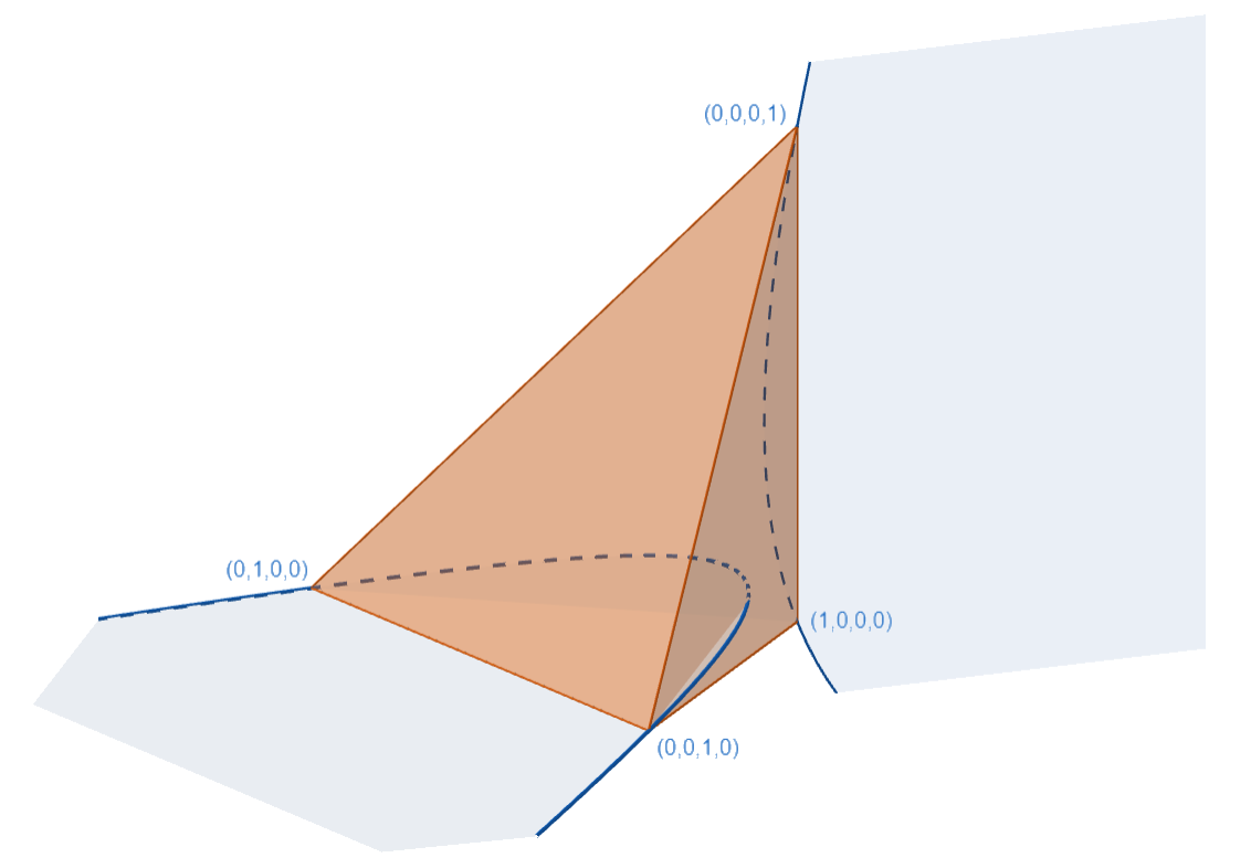
Figure 1. The real part of the Spohn variety $\mathcal{V}_{X}$ (blue lines) of “Prisoner’s Dilemma” and the tetrahedron $\overline{\Delta}$ of all strategies (orange). The vertices of $\overline{\Delta}$ are the pure strategies. Both components of $\mathcal{V}_{X}$ are plane conics. The game has two pure DE $(1,0,0,0)$ and $(0,0,0,1)$ attached to a curve segment of totally mixed DE, two isolated pure DE $(0,1,0,0)$ and $(0,0,1,0)$, and two mixed DE with one coordinate equal to $0$ which are attached to another curve segment of totally mixed DE.

Explanation 2.5 (concerning Theorem 3.2 and Corollary 3.4).

A game theorist would probably interpose in view of [10, Theorem 6]: I want to understand totally mixed dependency equilibria. These are at most the real points of the Spohn variety. So, what can you tell me about the real points, their dimension and degree? Are they an irreducible set?

In general, the set of points with real coordinates of a variety can have very strange properties. It might be even empty. However, the “in particular” of Theorem 3.2 tells us that for generic games $X$ (that is, again, for an open dense subset of the set of all games) the real part of the Spohn variety $\mathcal{V}_{X}$ is as large and looks structurally exactly as one would expect from looking at $\mathcal{V}_{X}$. Corollary 3.4 then uses this statement to infer for generic games that the set of real points on $\mathcal{V}_{X}$ is also irreducible, it has (real) dimension $s-(d_{1}+\ldots+d_{n}-n)$ and degree $d_{1}\cdots d_{n}$..

Explanation 2.6 (Three types of DE, Definition 3.6).

The notion of DE that we propose in Definition 3.6(1) keeps the conceptional game theoretic logic of Spohn’s original definition. It broadens the notion naturally in a purely mathematical manner by allowing, in order to approximate DE, instead of positive real points, as proposed by Spohn, arbitrary points for which the rational expressions $\mathbb{E}^{(i)}_{k}(p)$ defining DE are sensible. (2) Analytic DE is a notion that is intended to simplify the study of DE. (3) geometric DE are their algebro-geometric analogue. All three concepts turn out to be sensible in view of Corollary 3.11.

Explanation 2.7 (Bounds for the set of DE, Corollary 3.11).

Corollary 3.11 shows that an investigation of DE from the perspective of algebraic geometry is indeed sensible. Every DE is a positive real point on the Spohn variety $\mathcal{V}=\mathcal{V}_{X}$ and every strategy profile that lies on an irreducible component of the Spohn variety that contains a point, for which the rational expression $\mathbb{E}^{(i)}_{k}(p)$ of DE are well-defined, is a DE. The union of all such irreducible components is written as $\overline{\mathcal{V}\setminus\mathcal{W}}^{\text{Zar}}$ in Corollary 3.11 where $\mathcal{W}\subseteq\mathbb{P}^{d_{1}\times\ldots\times d_{n}-1}$ is the union of hyperplanes defined by the polynomial

$$s=\prod_{i,k}p_{+\ldots+k+\ldots+}.$$

These bounds are computationally very helpful because they can, given enough time, be computed by a computer algebra program such as Macaulay2. An explicit example of code for $(2\times 2)$-games is shown in Example 2.8 below.

We will see in Section 4 that none of the two bounds does necessarily agree with the set of DE. However, they do agree for generic games, which means for games outside of some algebraic variety of games. Here, we view the set of all $(d_{1}\times\cdots\times d_{n})$-games in normal form as the real vector space $\mathbb{R}^{n\times d_{1}\times\cdots\times d_{n}}$. It would be very interesting to explicitly determine this variety for games of a given size. We do this for $(2\times 2)$-games in Theorem 4.9, where this exceptional variety turns out to just be a union of hyperplanes in $\mathbb{R}^{8}$.

Example 2.8.

The following is a code for computations with the computer algebra software Macaulay2 [5] of lower and upper bounds for the set of DE of a $(2\times 2)$-game.

R is the polynomial ring whose variables are the four entries of a joint strategy of the players. aij and bij are the players’ payoffs, below for “Prisoner’s Dilemma”, which can be arbitrarily changed. V is the defining ideal (i.e., the set of defining polynomials) of the Spohn variety and W is the defining ideal of the four planes (whose union is $\mathcal{W}$) on which the rational expressions for DE are not defined.

componentsV lists all the systems of defining equations for the irreducible components of the Spohn variety. lowerBound computes the defining equations for the lower bound $\overline{\mathcal{V}\setminus\mathcal{W}}^{\text{Zar}}$. lowerBoundEqualsSpohn gives true or false according to whether $\overline{\mathcal{V}\setminus\mathcal{W}}^{\text{Zar}}=\mathcal{V}$ or not. In particular, in case true, the set of DE equals the Spohn variety. Finally, componentsLowerBound gives the list of all the systems of defining equations for the irreducible components of $\overline{\mathcal{V}\setminus\mathcal{W}}^{\text{Zar}}$. Note that this is a sublist of componentsV.

R = QQ[p11,p12,p21,p22];
a11 = -2;
a21 = -1;
a12 = -10;
a22 = -5;
b11 = -2;
b21 = -10;
b12 = -1;
b22 = -5;

V = ideal((p11+p12)*(a21*p21+a22*p22) - (p21+p22)*(a11*p11+a12*p12),
          (p11+p21)*(b12*p12+b22*p22) - (p12+p22)*(b11*p11+b21*p21));
W = ideal((p11+p12)*(p21+p22)*(p11+p21)*(p12+p22));

componentsV = minimalPrimes(V);
lowerBound = saturate(V,W);
lowerBoundEqualsSpohn = (V == lowerBound);
componentsLowerBound = minimalPrimes(lowerBound);

Example 2.9.

We consider the game

$$\begin{pmatrix}1&1\\ 2&-3\end{pmatrix}\text{ and }\begin{pmatrix}-1&0\\ 0&2\end{pmatrix}$$

from the class of games introduced in Example 4.4. The real part of its Spohn variety is shown in Figure 2. It is the union of two irreducible plane conics which intersect the set of all strategies $\overline{\Delta}$ exactly in the four pure strategies.

One of the irreducible components is contained in the exceptional planes whose union is $\mathcal{W}$. Hence, $\overline{\mathcal{V}\setminus\mathcal{W}}^{\text{Zar}}\neq\mathcal{V}$. The two pure strategies $(1,0,0,0)$ and $(0,0,1,0)$ lie in $\overline{\mathcal{V}\setminus\mathcal{W}}^{\text{Zar}}\cap\overline{\Delta}$ and are, therefore, DE. The other two pure strategies might be DE because they lie in $\mathcal{V}\cap\overline{\Delta}$ but further considerations are needed.

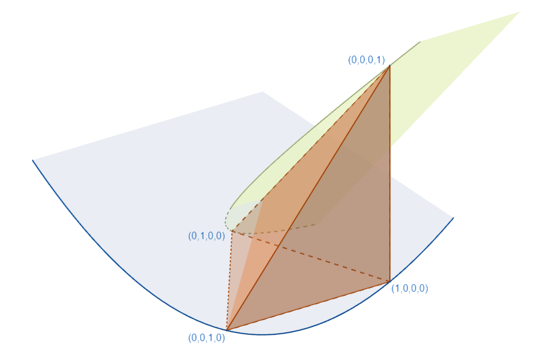
Figure 2. The real part of the Spohn variety of the $(2\times 2)$-game in Example 2.9. The lower bound $\overline{\mathcal{V}\setminus\mathcal{W}}^{\text{Zar}}$ is given by the blue line. But the Spohn variety has another irreducible component (green).

Explanation 2.10 (concerning Theorem 3.18 & Corollary 3.19).

For generic games (see Explanation 2.7), every NE is a DE by Corollary 3.19. What is more, for arbitrary games, every NE lies on the Spohn variety which is the algebraic model for the set of DE of a game (Theorem 3.18).

Figure 3 shows the Spohn variety consisting of four lines for the game

$$\begin{pmatrix}-1&-1\\ -2&3\end{pmatrix}\text{ and }\begin{pmatrix}-3&0\\ 0&0\end{pmatrix}.$$

The lower bound $\overline{\mathcal{V}\setminus\mathcal{W}}^{\text{Zar}}$ for DE equals the blue component. By Example 4.7, the blue point is a NE but not a dependency equilibrium. This is only possible because it lies on one of the green components of $\mathcal{V}$. These are exactly the components of $\mathcal{V}$ that are contained in $\mathcal{W}$.

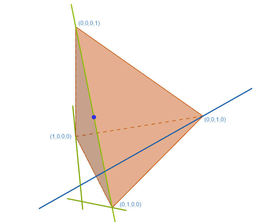
Figure 3. The Spohn variety of the game from Explanation 2.10. The blue point is a NE but not a DE. The blue line goes along one of the faces of the tetrahedron. One of the three green lines passes along an edge.

Explanation 2.11 (concerning Proposition 3.21).

The proposition gives a criterion, in terms of linear algebra, for the existence of a whole family of totally mixed DE around a pure strategy. This criterion also serves as a sufficient condition for the existence of a pure DE.

The criterion is based on the Jacobian matrix of the Spohn variety at a pure strategy, which is analysed in Remark 3.20. Clearly, it is only of theoretic value without further investigations of the Jacobian. But, in principle, this can be done, as Example 4.8 shows. There, we give a very explicit form of this criterion for $(2\times 2)$-games involving only equalities and inequalities in the entries of the payoff tables. Figure 1 shows the Spohn variety of an example of a game where this criterion applies for the pure strategies $(1,0,0,0)$ and $(0,0,0,1)$, but it fails for the other two pure strategies, although these are also DE.

Explanation 2.12 (concerning Theorem 4.2).

$(2\times 2)$-games split up into distinct classes concerning the geometric structure of their sets of DE. An understanding of these classes is based on the considerations of Theorem 4.2 and its proof which give, from this viewpoint, a full and sensible characterization of $(2\times 2)$-games. Cases (3)(c) and (3)(d) deserve further investigation concerning the number of irreducible components of the Spohn variety (which all are curves in these cases) and their individual degrees. This is studied in an ongoing project [9].

3. Results for arbitrary games

Real points of the Spohn variety

In the following, we want to show that the Spohn variety $\mathcal{V}=\mathcal{V}_{X}$ of a game $X$, that is, the variety of all complex projective points satisfying the equations of a dependency equilibrium (see [10, (4)]), always has smooth points with real coordinates. This enables us to apply the following result which, in turn, makes it possible to study the set of all dependency equilibria from the point of view of complex projective varieties. As a consequence, we can apply the results of [10] to the case that is actually relevant for game-theoretical applications.

Fact 3.1.

[8, Theorem 2.2.9] Let $V$ be an irreducible complex affine variety defined by real polynomials. If $V$ contains a smooth point with real coordinates then $V(\mathbb{R})$, the set of real points of $V$, lies Zariski dense in $V$.

We can apply this by taking a dense open affine subset of the ambient projective space and thereby assuming that $V=\mathcal{V}$ is affine.

Theorem 3.2.

For an arbitrary game $X$, the Spohn variety $\mathcal{V}=\mathcal{V}_{X}$ contains a smooth point with real coordinates. In particular, if $\mathcal{V}$ is irreducible then its set of real points lies Zariski dense in $\mathcal{V}$.

Proof.

For $(2\times 2)$-games, this is just Proposition 4.1.

In all other cases, we use the vector bundle parametrization $\phi:\mathcal{V}_{X}\dashrightarrow(\mathbb{P}^{1})^{n}$ of the proof of [10, Theorem 8] and can write

$$\mathcal{V}=\{p\mid K_{X}(z)\cdot p=0\text{ for some }z\in(\mathbb{P}^{1})^{n}\},$$

where $K_{X}(z)$ is the Konstanz matrix of the game $X$, as defined in [10]. Its entries are real numbers when $z$ has real coordinates. Note that the standing assumption of [10] that the payoff tables of the game being generic is not necessary for the construction of the map.

Take a real point $z$ in the image of $\phi$ such that $\phi^{-1}(\{z\})$ is not contained in the singular locus of $\mathcal{V}$. Now, as $\phi^{-1}(\{z\})=\{p\mid K_{X}(z)\cdot p=0\}$ is the kernel of a real matrix it contains real points and, hence, also a smooth real point of $\mathcal{V}$. ∎

Regarding game-theoretic applications, it might be interesting to find smooth real points on every irreducible component of the Spohn variety of a game. The question below asks exactly for this generalization of Theorem 3.2,

Question 3.3.

Does every irreducible component of the Spohn variety of a game contain a smooth real point?

The following is the combination of Theorem 3.2 with [10, Theorem 6].

Corollary 3.4.

The set of real points of the Spohn variety of a game has the following properties generically: It is irreducible, of codimension $d_{1}+\ldots+d_{n}-n$ and degree $d_{1}\cdots d_{n}$.

Passing to boundary cases

In this section, we change loosely between the projective setting of the Spohn variety and the affine setting of points in $\mathbb{C}^{d_{1}\times\ldots\times d_{n}}$. Namely, if some definition depends on the choice of the affine representative of a projective point, we always take the representative whose entries sum up to $1$, as is customary in the setting of probability distributions and strategies of games.

The definition of DE used in [10] lets points on the relative boundary of $\Delta$ unregarded. We denote by $\overline{\Delta}$ the relative closure of $\Delta$, that is, the set of all joint strategies of the players, while $\Delta$ is just the set of totally mixed strategies.

Spohn [13, 14] defines DE as points $p=(p_{j_{1}\ldots j_{n}})$ in $\overline{\Delta}$ that are limits of sequences $(p^{(r)})_{r\in\mathbb{N}}$ in $\Delta$ satisfying

(1) $$\lim_{r\to\infty}\mathbb{E}^{(i)}_{k}(p^{(r)})=\lim_{r\to\infty}\mathbb{E}^{(i)}_{k^{\prime}}(p^{(r)})$$

for all $i\in\{1,\ldots,n\}$ and $k,k^{\prime}\in\{1,\ldots,d_{i}\}$. In the special case of $(2\times 2)$-games with the notation of [10, Example 2], these conditions read as follows:

$$\lim_{r\to\infty}\frac{a_{11}p^{(r)}_{11}+a_{12}p^{(r)}_{12}}{p^{(r)}_{11}+p^{(r)}_{12}} =\lim_{r\to\infty}\frac{a_{21}p^{(r)}_{21}+a_{22}p^{(r)}_{22}}{p^{(r)}_{21}+p^{(r)}_{22}}$$

$$\lim_{r\to\infty}\frac{b_{11}p^{(r)}_{11}+b_{21}p^{(r)}_{21}}{p^{(r)}_{11}+p^{(r)}_{21}} =\lim_{r\to\infty}\frac{b_{12}p^{(r)}_{12}+b_{22}p^{(r)}_{22}}{p^{(r)}_{12}+p^{(r)}_{22}}$$

Spohn then claims in [14, Section 4, Observation 3] that, with this definition, every Nash equilibrium (NE) is a DE. This is true, in principle, but not in general, as we want to illustrate with the next example.

Example 3.5 (Bach or Stravinski).

We use the payoff tables $(2,0,0,1)$ and $(1,0,0,2)$ as in [14, Section 3]. The equations (1) translate as

$$\lim_{r\to\infty}\frac{2p^{(r)}_{11}}{p^{(r)}_{11}+p^{(r)}_{12}} =\lim_{r\to\infty}\frac{p^{(r)}_{22}}{p^{(r)}_{21}+p^{(r)}_{22}},$$

$$\lim_{r\to\infty}\frac{p^{(r)}_{11}}{p^{(r)}_{11}+p^{(r)}_{21}} =\lim_{r\to\infty}\frac{2p^{(r)}_{22}}{p^{(r)}_{12}+p^{(r)}_{22}}.$$

First, we want to note that [14, Section 3] does not contain the DE of the form $(0,1-x,x,0)$ for $0\leq x\leq 1$. The two special ones with $x\in\{0,1\}$ can be reached as limits of those with $0<x<1$ for which the above equation hold even without limits. Second, we point out that the two NE $(1,0,0,0)$ and $(0,0,0,1)$ cannot be approximated by points in $\Delta$ satisfying the equations above. Indeed, assume to the contrary that the sequence $p^{(r)}$ converges to $(1,0,0,0)$ and the above equations are satisfied. Then, $\lim_{r\to\infty}p_{11}^{(r)}=1$ and all other $p_{ij}^{(r)}$ converge to $0$. This means that $\lim_{r\to\infty}\frac{2p^{(r)}_{11}}{p^{(r)}_{11}+p^{(r)}_{12}}=2=\lim_{r\to\infty}\frac{p^{(r)}_{22}}{p^{(r)}_{21}+p^{(r)}_{22}}$. Since all the $p_{ij}^{(r)}$ are strictly positive, it follows that $\frac{1}{2}=\lim_{r\to\infty}\frac{p^{(r)}_{21}+p^{(r)}_{22}}{p^{(r)}_{22}}=\lim_{r\to\infty}\frac{p^{(r)}_{21}}{p^{(r)}_{22}}+1$. So $\lim_{r\to\infty}\frac{p^{(r)}_{21}}{p^{(r)}_{22}}=-\frac{1}{2}$ and hence this last sequence must get negative for $r$ sufficiently large. This is a contradiction to $p_{ij}^{(r)}>0$.

We now give a slightly more general definition for DE, so that every NE is a DE for generic games. Additionally, we define two further equilibrium concepts and then want to investigate the relations between all of them. The final goal would be to show (if true) that all three concepts coincide which would make DE (in our sense) computable by symbolic methods. But first, we need some notation. Let $X$ be a game given in normal form by its payoff tensors $(X^{(i)}_{j_{1}\ldots j_{n}})$, $\mathcal{V}=\mathcal{V}_{X}\subseteq\mathbb{P}^{d_{1}\times\ldots\times d_{n}-1}$ the Spohn variety of $X$ and $\mathcal{I}=\mathcal{I}_{X}$ its ideal in the polynomial ring $R=\mathbb{C}[p_{j_{1}\ldots j_{n}}\mid j_{i}\in\{1,\ldots,d_{i}\}]$. Moreover, let $\mathcal{W}\subseteq\mathbb{P}^{d_{1}\times\ldots\times d_{n}-1}$ be the union of hyperplanes defined by the polynomial

$$s=\prod_{i,k}p_{+\ldots+k+\ldots+}.$$

For a subset $M\subseteq\mathbb{C}^{d_{1}\times\ldots\times d_{n}}$ (respectively $\mathbb{P}^{d_{1}\times\ldots\times d_{n}-1}$ or $\mathbb{R}^{d_{1}\times\ldots\times d_{n}}$), we denote by $\overline{M}$ its usual euclidean closure, that is, the set of all points that are limits of sequences in $M$, and by $\overline{M}^{\text{Zar}}$ its Zariski closure, that is, the set of all points that are common zeros of polynomials vanishing on $M$. It is a basic fact that $\overline{M}\subseteq\overline{M}^{\text{Zar}}$ because every algebraic set is closed in the euclidean topology.

Definition 3.6.

1. A dependency equilibrium (DE) is a point $p$ in $\overline{\Delta}$ such that there exists a sequence $(p^{(r)})$ of complex tensors in the complement of $\mathcal{W}$ (that is, $s(p^{(r)})\neq 0$ for all $r$) converging to $p$ such that the equations in (1) are satisfied.

2. An analytic dependency equilibrium (aDE) is a point in $\overline{\Delta}\cap\overline{(\mathcal{V}\setminus\mathcal{W})}$.

3. A geometric dependency equilibrium (gDE) is a point in $\overline{\Delta}\cap\overline{(\mathcal{V}\setminus\mathcal{W})}^{\text{Zar}}$.

For generic games, we can replace complex tensors by real tensors in Definition 3.6 and still deduce results analogous to the contents of this section, see Remark 3.12.

Remark 3.7.

1. Every aDE clearly is a DE because it can be approximated by a sequence in $\mathcal{V}\setminus\mathcal{W}$. In symbols, aDE $\subseteq$ DE.

2. Every aDE is a gDE because $\overline{(\mathcal{V}\setminus\mathcal{W})}\subseteq\overline{(\mathcal{V}\setminus\mathcal{W})}^{\text{Zar}}$. In symbols, aDE $\subseteq$ gDE.

For all $(2\times 2)$-games in [14, Section 3] (Matching pennies, Bach or Stravinski, Hawk and Dove, Prisoner’s Dilemma), the three concepts of DE, aDE and gDE coincide.

Cases where DE concide with gDE are particularly nice from the view point of game-theoretic applications of the theory of DE because we can describe DE by methods from computational commutative algebra there: Computer algebra software like Macaulay2 can compute for us the minimal prime ideals of the saturated ideal $(\mathcal{I}_{X}:s^{\infty})$. The generators of these minimal primes exactly give the equations for the irreducible components of $\overline{(\mathcal{V}\setminus\mathcal{W})}^{\text{Zar}}$. The only humanly task is then to figure out which points in $\overline{\Delta}$ satisfy these equations that are very easy in many cases. The next proposition tells us that a large class of DE always can be computed in this way.

Proposition 3.8.

For every game, aDE and gDE coincide.

Proof.

In [7, Exposé XII, Prop. 2.2], if we take $\mathcal{V}$ as the $\mathbb{C}$-scheme $X$ and $T=\mathcal{V}\setminus\mathcal{W}$ the locally constructible subset (that is actually a Zariski open subset) then this proposition just says that $\overline{\mathcal{V}\setminus\mathcal{W}}^{\text{Zar}}=\overline{\mathcal{V}\setminus\mathcal{W}}$. This immediately implies our assertion. ∎

Remark 3.9.

The set $\overline{\Delta}\cap(\mathcal{V}\setminus\mathcal{W})$ consists of all DE not in $\mathcal{W}$ because for points outside of $\mathcal{W}$ all the expressions $p_{+\ldots+k+\ldots+}$ are non-zero.

Theorem 3.10.

Every dependency equilibrium of a game $X$ lies on $\mathcal{V}_{X}$, the Spohn variety of $X$.

Proof.

Let $p$ be a DE of $X$ and $p^{(r)}$ a sequence in $\mathbb{C}^{d_{1}\times\ldots\times d_{n}}\setminus\mathcal{W}$ such that $\sum p^{(r)}_{j_{1}\ldots j_{n}}=1$, $\lim_{r\to\infty}p^{(r)}=p$, and the equations (1) are satisfied. We show that $p$ satisfies every defining equation of the Spohn variety. For each player $i$ and each pair $k,k^{\prime}$ of pure strategies, we get the equation

$$p_{+\ldots+k^{\prime}+\ldots+}\sum_{j_{1},\ldots,j_{i-1},j_{i+1},\ldots,j_{n}}X^{(i)}_{j_{1}\ldots k\ldots j_{n}}p_{j_{1}\ldots k\ldots j_{n}}=p_{+\ldots+k+\ldots+}\sum_{j_{1},\ldots,j_{i-1},j_{i+1},\ldots,j_{n}}X^{(i)}_{j_{1}\ldots k^{\prime}\ldots j_{n}}p_{j_{1}\ldots k^{\prime}\ldots j_{n}}.$$

If $p_{+\ldots+k+\ldots+}=0$ then all $p_{j_{1}\ldots k\ldots j_{n}}$ are $0$ and the equation above is trivially satisfied. The same is true for $k^{\prime}$ in place of $k$. If, on the other hand, $p_{+\ldots+k+\ldots+}\neq 0$ and $p_{+\ldots+k^{\prime}+\ldots+}\neq 0$ then the limits $\lim_{r\to\infty}p_{+\ldots+k+\ldots+}^{(r)}=p_{+\ldots+k+\ldots+}\neq 0$ and $\lim_{r\to\infty}p_{+\ldots+k^{\prime}+\ldots+}^{(r)}=p_{+\ldots+k^{\prime}+\ldots+}\neq 0$ and the equation above is equivalent to the corresponding equation in (1). ∎

Corollary 3.11.

For the set $\text{DE}(X)$ of dependency equilibria of a game $X$, there are inclusions

$$\overline{\Delta}\cap\overline{\mathcal{V}\setminus\mathcal{W}}^{\text{Zar}}=\overline{\Delta}\cap\overline{\mathcal{V}\setminus\mathcal{W}}\subseteq\text{DE}(G)\subseteq\overline{\Delta}\cap\mathcal{V},$$

where $\mathcal{V}=\mathcal{V}_{X}$ is the Spohn variety of $X$. Both inclusions can be strict in general, see Section 4.

Remark 3.12.

Corollary 3.11 is still valid for generic games when one replaces complex tensors by real tensors in Definition 3.6(1). In other words, for generic games $X$, the following three statements are equivalent for a strategy $p$:

1. $p$ is a DE of $X$ in the sense of Definition 3.6(1).

2. There exists a sequence $(p^{(r)})$ of real tensors in the complement of $\mathcal{W}$ (that is, $s(p^{(r)})\neq 0$ for all $r$) converging to $p$ such that the equations in (1) are satisfied.

3. $p$ lies on the Spohn variety of $X$.

Proof.

For generic games, the Spohn variety $\mathcal{V}$ is irreducible and not contained in $\mathcal{W}$. Hence, (a) and (c) are equivalent. Moreover, the implication from (b) to (a) is trivial.

For the remaining implication from (a) to (b), it is sufficient to show that $\overline{\mathcal{V}\setminus\mathcal{W}}\cap\overline{\Delta}$ (which coincides with $\text{DE}(G)$ for generic games) is contained in the set $\text{DE}_{\mathbb{R}}(G)$ of all points satisfying the statement in (b). For this, it suffices to show the equality

(2) $$\overline{\mathcal{V}\setminus\mathcal{W}}\cap\mathbb{R}^{s}=\overline{(\mathcal{V}\setminus\mathcal{W})\cap\mathbb{R}^{s}},$$

where $s$ is the dimension of the ambient space. Indeed, if we intersect the right side of (2) with $\overline{\Delta}$ then the resulting set is contained in $\text{DE}_{\mathbb{R}}(G)$, because $(\mathcal{V}\setminus\mathcal{W})\cap\mathbb{R}^{s}$ consists of real tensors satisfying the defining rational equations for DE.

To show (2), note that $\overline{\mathcal{V}(\mathbb{R})\setminus\mathcal{W}(\mathbb{R})}$ is a real variety contained in the real variety $\overline{\mathcal{V}\setminus\mathcal{W}}\cap\mathbb{R}^{s}$ and both have the same dimension because $\mathcal{V}(\mathbb{R})$ lies Zariski dense in $\mathcal{V}$ by Theorem 3.2. Therefore, they are the same. Also, $\mathcal{V}(\mathbb{R})\setminus\mathcal{W}(\mathbb{R})=(\mathcal{V}\setminus\mathcal{W})\cap\mathbb{R}^{s}$ is always true for set-theoretical reasons and, therefore, (2) follows. ∎

Remark 3.13.

That (2) is not true in general for an algebraic variety $\mathcal{V}$ and a union of hyperplanes $\mathcal{W}$ can be seen by the following example: Let $\mathcal{V}$ be an irreducible complex surface of degree greater than $1$ whose real part is just a line. For instance, consider the surface in complex affine $3$-space defined by the equation

$$2x^{2}+2xy+y^{2}-2xz-2yz+z^{2}-2x+1=0.$$

Its set of real points is the line defined by

$$y-z+1=x-1=0.$$

If now $\mathcal{W}$ is a hyperplane containing this line then $\overline{\mathcal{V}\setminus\mathcal{W}}=\mathcal{V}$ and hence $\overline{\mathcal{V}\setminus\mathcal{W}}\cap\mathbb{R}^{s}=\mathcal{V}(\mathbb{R})$ which is the line. But $(\mathcal{V}\setminus\mathcal{W})\cap\mathbb{R}^{s}$ is the empty set, so (2) does not hold.

Remark 3.14.

In view of Corollary 3.11, it might be interesting to understand for which games the equality $\overline{\mathcal{V}\setminus\mathcal{W}}^{\text{Zar}}=\mathcal{V}$ holds. Indeed, in these cases, the set of DE coincides with $\overline{\Delta}\cap\mathcal{V}$. In general, $\overline{\mathcal{V}\setminus\mathcal{W}}^{\text{Zar}}=\mathcal{V}$ if and only if no irreducible component of $\mathcal{V}$ is contained in $\mathcal{W}$.

A game $X$ (of a fixed size) given in normal form by its payoff tables $(X^{(i)}_{j_{1}\ldots j_{n}})_{(j_{1},\ldots,j_{n})\in d_{1}\times\ldots\times d_{n}}$, $i=1,\ldots,n$, is nothing else than a point in the affine space $\mathbb{R}^{n\times d_{1}\times\ldots\times d_{n}}\subseteq\mathbb{C}^{n\times d_{1}\times\ldots\times d_{n}}$. So we could ask for a structural result on the set of all affine points $X\in\mathbb{R}^{n\times d_{1}\times\ldots\times d_{n}}$ such that $\mathcal{V}_{X}\setminus\mathcal{W}$ lies (Zariski) dense inside $\mathcal{V}_{X}$.

Proposition 3.15.

The set $\mathcal{X}$ of all games $X\in\mathbb{R}^{n\times d_{1}\times\ldots\times d_{n}}$ such that $\overline{\mathcal{V}_{X}\setminus\mathcal{W}}^{\text{Zar}}=\mathcal{V}_{X}$ (which implies that the set of dependency equilibria of $X$ coincides with the non-negative real part of $\mathcal{V}_{X}$) is the complement of an affine variety in $\mathbb{R}^{n\times d_{1}\times\ldots\times d_{n}}$. In particular, it is a dense subset of $\mathbb{R}^{n\times d_{1}\times\ldots\times d_{n}}$.

Proof.

We use [6, Prop. 9.5.3]. We consider the $\mathbb{C}$-algebras

$$\mathcal{A}=\mathbb{C}[X^{(i)}_{j_{1}\ldots j_{n}}\mid i\in\{1,\ldots,n\},(j_{1},\ldots,j_{n})\in[d_{1}]\times\ldots\times[d_{n}]]$$

and

$$\mathcal{B}=\frac{\mathbb{C}[X^{(i)}_{j_{1}\ldots j_{n}},p_{j_{1},\ldots,j_{n}}\mid i\in\{1,\ldots,n\},(j_{1},\ldots,j_{n})\in[d_{1}]\times\ldots\times[d_{n}]]}{\mathcal{I}_{X}},$$

where the $X^{(i)}_{j_{1}\ldots j_{n}}$ are variables for the entries of the payoff tables, the $p_{j_{1},\ldots,j_{n}}$ are variables for the entries of a strategy and $\mathcal{I}_{X}$ is the ideal generated by the polynomials of the defining equation of the Spohn variety (with variable payoff tables). A $\mathbb{C}$-algebra homomorphism $\mathcal{A}\to\mathcal{B}$ is given by composing the canonical inclusion

$$\mathcal{A}\to\mathbb{C}[X^{(i)}_{j_{1}\ldots j_{n}},p_{j_{1},\ldots,j_{n}}\mid i\in\{1,\ldots,n\},(j_{1},\ldots,j_{n})\in[d_{1}]\times\ldots\times[d_{n}]]$$

with the projection

$$\mathbb{C}[X^{(i)}_{j_{1}\ldots j_{n}},p_{j_{1},\ldots,j_{n}}\mid i\in\{1,\ldots,n\},(j_{1},\ldots,j_{n})\in[d_{1}]\times\ldots\times[d_{n}]]\to\mathcal{B}.$$

From this, we get an induced finitely presented morphism $f$ of affine schemes $T:=\operatorname{Spec}(\mathcal{B})\to\operatorname{Spec}(\mathcal{A})=:S$ and the fibre (intersected with $\operatorname{Max}(\mathcal{B})$) of a point $X\in\mathbb{C}^{n\times d_{1}\times\ldots\times d_{n}}=\operatorname{Max}(\mathcal{A})$ is the Spohn variety of $X$. So, $f$ parametrizes the family of all Spohn varieties along the set of all games of the fixed size $n\times d_{1}\times\ldots\times d_{n}$.

We derive the closed subscheme $\mathcal{W}$ of $X$ from the projection $\mathcal{B}\to\mathcal{B}/(s)$, where

$$s=\prod_{i,k}p_{+\ldots+k+\ldots+}.$$

We set $Z=T\setminus\mathcal{W}$ and $Z^{\prime}=T$. Now, for any $X\in\operatorname{Max}(\mathcal{A})$, $Z^{\prime}\cap f^{-1}(X)=\mathcal{V}_{X}$ and $Z\cap f^{-1}(X)=\mathcal{V}_{X}\setminus\mathcal{W}$. With this in mind, the set $\mathcal{X}$ of the games in question is a constructible set by [6, Prop. 9.5.3], using exactly the same notation.

It is immediate from the computations of the Jacobian matrix of $\mathcal{V}_{X}$ in Remark 3.20 that the set of all games $X$ such that $\mathcal{V}_{X}$ intersects all irreducible components of $\mathcal{W}$ transversally is Zariski open. But this set is clearly contained in $\mathcal{X}$. So $\mathcal{X}$ is a constructible set in an affine space containing a Zariski open set and it is therefore itself Zariski open, that is, the complement of an affine variety. ∎

Problem 3.16.

For fixed $n$ and $d_{1},\ldots,d_{n}$, describe the Zariski open set $\mathcal{X}$ (see Prop. 3.15), that is, give the defining equations of its complement.

The solution of this problem for $(2\times 2)$-games is Theorem 4.9.

Nash equilibria and the Spohn variety

Now, we want to give a first application of the lower and upper bounds for dependency equilibria from Corollary 3.11. It shows that, in reasonable situations, every Nash equilibrium is a dependency equilibria. By Example 4.7, although this is not always the case, by Theorem 3.18, every Nash equilibrium lies on the Spohn variety.

Note that the totally mixed Nash equilibria are exactly the positive real points that lie both on the Spohn variety and on the Segre variety by a result of Sturmfels and the first author [10, Theorem 6]. In particular, totally mixed Nash equilibria are always dependency equilibria.

By $\Delta_{d-1}$ we denote the $(d-1)$-dimensional standard simplex. It can be considered as a subset of a $d$-dimensional affine space or of a $(d-1)$-dimensional projective space.

Lemma 3.17.

A rank-one point $p=(p_{1}^{(1)},\ldots,p_{d_{1}}^{(1)},\ldots\ldots,p_{1}^{(n)},\ldots,p_{d_{n}}^{(n)})\in\Delta_{d_{1}-1}\times\ldots\times\Delta_{d_{n}-1}\subseteq\overline{\Delta}$ lies on the Spohn variety of the game $X$ if and only if

(3) $$\sum_{j_{1}=1}^{d_{1}}\ldots\sum_{j_{i-1}=1}^{d_{i-1}}\sum_{j_{i+1}=1}^{d_{i+1}}\ldots\sum_{j_{n}=1}^{d_{n}}\left(X^{(i)}_{j_{1}\ldots j_{i-1}kj_{i+1}\ldots j_{n}}-X^{(i)}_{j_{1}\ldots j_{i-1}k^{\prime}j_{i+1}\ldots j_{n}}\right)p_{j_{1}}^{(1)}\cdots p_{j_{i-1}}^{(i-1)}p_{j_{i+1}}^{(i+1)}\cdots p_{j_{n}}^{(n)}=0$$

for all $i\in\{1,\ldots,n\}$ and all $k,k^{\prime}\in\{1,\ldots,d_{i}\}$ with $p_{k}^{(i)}>0$ and $p_{k^{\prime}}^{(i)}>0$.

Proof.

To recover the notation for general tensors on the Spohn variety, we set $p_{j_{1}\ldots j_{n}}=p_{j_{1}}^{(1)}\cdots p_{j_{n}}^{(n)}$. Note that $p_{+\ldots+k+\ldots+}=p_{k}^{(i)}$ for all $i$ and $k$. Let $i\in\{1,\ldots,n\}$ and $k,k^{\prime}\in\{1,\ldots,d_{i}\}$. If $p_{k}^{(i)}=0$ or $p_{k^{\prime}}^{(i)}=0$ then the corresponding defining equation for the Spohn variety is trivial. So, assume that both are non-zero. Then the corresponding defining equation of the Spohn variety boils down for rank-one tensors to (3), as noted in the proof of [10, Theorem 6]. ∎

Theorem 3.18.

Every Nash equilibrium of a game $X$ lies on $\mathcal{V}_{X}$, the Spohn variety of $X$.

Proof.

We use the notation of Lemma 3.17 for the given Nash equilibrium $p$ of $X$. If $p_{k}^{(i)}=0$ or $p_{k^{\prime}}^{(i)}=0$ then the corresponding defining equation for the Spohn variety is trivial. In the case that both are non-zero, it is a simple computation that the equations of [15, Theorem 6.6] are equivalent to (3), and hence $p$ lies on $\mathcal{V}_{X}$. ∎

Corollary 3.19.

If the variety $\mathcal{W}$ contains no irreducible component of the Spohn variety $\mathcal{V}_{X}$ of a game $X$ then every Nash equilibrium of $X$ is a dependency equilibrium of $X$.

In particular, when the payoff tables of $X$ are generic, every Nash equilibrium of $X$ is a dependency equilibrium of $X$.

Proof.

This follows from Theorem 3.18 in combination with Remark 3.14. ∎

Existence of pure and totally mixed DE

We now employ an easy idea from algebraic geometry to find large collections of games that admit infinitely many totally mixed DE. Our method will then guarantee, in addition, the existence of a pure DE.

Remark 3.20.

Let $\mathcal{V}$ be the Spohn variety of a game given by its payoff tensors $(X^{(i)}_{j_{1}\ldots j_{n}})$. The rows of the Jacobian matrix $\mathcal{J}(p)$ of $\mathcal{V}$ at a point $p=(p_{j_{1}\ldots j_{n}})$ has row indices $(i,k,k^{\prime})$ with $1\leq i\leq n$ and $1\leq k<k^{\prime}\leq d_{i}$ (corresponding to the defining equations of $\mathcal{V}$) and column indices $(r_{1},\ldots,r_{n})$ where $1\leq r_{j}\leq d_{j}$ (corresponding to the partial derivative at the variable $p_{r_{1}\ldots r_{n}}$). The entry with this row and column index is $0$ unless $r_{i}\in\{k,k^{\prime}\}$. In these cases, it is

$$p_{+\ldots+k+\ldots+}X^{(i)}_{r_{1}\ldots k^{\prime}\ldots r_{n}}-\sum_{j_{1},\ldots,j_{i-1},j_{i+1},\ldots,j_{n}}X^{(i)}_{j_{1}\ldots k\ldots j_{n}}p_{j_{1}\ldots k\ldots j_{n}}$$

and

$$\sum_{j_{1},\ldots,j_{i-1},j_{i+1},\ldots,j_{n}}X^{(i)}_{j_{1}\ldots k^{\prime}\ldots j_{n}}p_{j_{1}\ldots k^{\prime}\ldots j_{n}}-p_{+\ldots+k^{\prime}+\ldots+}X^{(i)}_{r_{1}\ldots k\ldots r_{n}},$$

respectively.

If $p$ is now the pure strategy that has a $1$ at position $(j_{1},\ldots,j_{i-1},k^{\prime},j_{i+1},\ldots,j_{n})$ and $0$ elsewhere then an entry of $\mathcal{J}(p)$ is $0$ unless $r_{i}=k$. The entry in row $(i,k,k^{\prime})$ and column $(r_{1},\ldots,r_{i-1},k,r_{i+1},\ldots,r_{n})$ equals

$$X^{(i)}_{j_{1}\ldots k^{\prime}\ldots j_{n}}-X^{(i)}_{r_{1}\ldots k\ldots r_{n}}.$$

Note that the pure strategy $p$ always lies on $\mathcal{V}$ by definition.

Proposition 3.21.

Suppose that the Spohn variety $\mathcal{V}$ of a game $X$ is smooth at the pure strategy $p$, that is, its Jacobian $\mathcal{J}(p)$ at $p$ (see Remark 3.20) has maximal possible rank. Then the following are equivalent

1. Every (euclidean) neighbourhood of $p$ contains a totally mixed dependency equilibrium of $X$.

2. The kernel of $\mathcal{J}(p)$ contains a vector all of whose entries are positive real numbers.

In this case, $p$ is a pure dependency equilibrium of $X$.

Proof.

The kernel of $\mathcal{J}(p)$ shifted by $p$, that is, $\ker\mathcal{J}(p)+p$ is the tangent space of $\mathcal{V}$ at $p$. As the column $(r_{1},\ldots,k^{\prime},\ldots,r_{n})$ of $\mathcal{J}(p)$ consists of zeros, $\ker\mathcal{J}(p)$ contains a vector with all entries positive if and only if this tangent space does. This is the case if and only if the tangent space has non-empty intersection with $\Delta$ which is true exactly when $\mathcal{V}\cap U\cap\Delta\neq\emptyset$ for every (euclidean) neighbourhood $U$ around $p$. This, in turn, is equivalent to (1) in the statement of the proposition.

As $\mathcal{V}\cap U\cap\Delta\neq\emptyset$ for every neighbourhood $U$ of $p$, a whole irreducible component of $\mathcal{V}$ containing $p$ passes through $\Delta$ and is therefore not contained in $\mathcal{W}$. It follows by Corollary 3.11 that $p$ is a DE. ∎

Remark 3.22.

1. Clearly, the method of the proof of Proposition 3.21 works for arbitrary $p\in\overline{\Delta}$ that is a smooth point of $\mathcal{V}$: Every euclidean neighbourhood of $p$ contains a DE of $X$ if and only if $\ker\mathcal{J}(p)+p$ contains a positive vector.

2. Even if this is not true, one might find out that $p$ is a DE of $X$ by checking that $\ker\mathcal{J}(p)+p$ is not contained in $\mathcal{W}$.

3. If $\ker\mathcal{J}(p)+p\subseteq\mathcal{W}$ it could still be possible to find out that $p$ is a DE of $X$ by exhibiting that an irreducible component of $\mathcal{V}$, containing $p$ as a smooth point, is not linear, for instance, by studying second order derivatives of $\mathcal{V}$ around $p$.

Even though the structure of $\mathcal{J}(p)$ is very simple for a pure strategy $p$, see Remark 3.20, which is helpful for concrete applications of Proposition 3.21, it is in general hard to derive a sensible general sufficient condition for the existence of DE around $p$ from it. However, it is possible for games of small size, such as $(2\times 2)$-games, see Example 4.8.

4. General results for $(2\times 2)$-games

Next, we exhibit when at least one of the four pure strategies is a smooth point on the Spohn variety of a game. Note that these points are always on the variety.

Proposition 4.1.

The Spohn variety of the $(2\times 2)$-game

$$\begin{pmatrix}a_{11}&a_{12}\\ a_{21}&a_{22}\end{pmatrix}\text{ and }\begin{pmatrix}b_{11}&b_{12}\\ b_{21}&b_{22}\end{pmatrix}$$

contains $p=(1,0,0,0)$ as a smooth point if and only if one of the following holds:

1. $a_{11}\neq a_{21}$ and $b_{11}\neq b_{12}$

2. $a_{11}=a_{21}$, $a_{11}\neq a_{22}$ and $b_{11}\neq b_{12}$

3. $b_{11}=b_{12}$, $b_{11}\neq b_{22}$ and $a_{11}\neq a_{21}$.

One of the four pure strategies is always a smooth point on the Spohn variety.

Proof.

The Jacobian of the Spohn variety at $p$ is

$$\mathcal{J}(p)=\begin{pmatrix}0&a_{11}-a_{21}&0&a_{11}-a_{22}\\ 0&0&b_{11}-b_{12}&b_{11}-b_{22}\end{pmatrix}.$$

By considering analogous characterizations for the other pure strategies, it can be easily checked that at least one of the four pure strategies is a smooth point, unless the pay-off tables are of the form shown in Theorem 4.2(3)(a) in which case the Spohn variety is smooth anyway. ∎

Theorem 4.2.

There are the following cases for the Spohn variety $\mathcal{V}$ of the $(2\times 2)$-game

$$\begin{pmatrix}a_{11}&a_{12}\\ a_{21}&a_{22}\end{pmatrix}\text{ and }\begin{pmatrix}b_{11}&b_{12}\\ b_{21}&b_{22}\end{pmatrix}.$$

1. Both payoff tables are constant in which case $\mathcal{V}=\mathbb{P}^{3}$.

2. Exactly one of the payoff tables is constant.

   • $\mathcal{V}$ is an irreducible surface of degree $2$ and so is its real part.

   • $\mathcal{V}$ is the union of two distinct planes and so is its real part.

3. None of the payoff tables is constant.

   • The payoff tables are of the form

     $$\begin{pmatrix}a&c\\ a&c\end{pmatrix}\text{ and }\begin{pmatrix}b&b\\ d&d\end{pmatrix}$$

     with $a\neq c$ and $b\neq d$. Then $\mathcal{V}$ is an irreducible surface of degree $2$, the Segre variety in $\mathbb{P}^{3}$, and so is its real part.

   • $\mathcal{V}$ is the intersection of two varieties which are both the union of two distinct planes.

     • $\mathcal{V}$ is the union of a plane and a line not contained in the plane, and so is its real part.

     • $\mathcal{V}$ is the union of two lines with empty intersection, and so is its real part.

   • $\mathcal{V}$ is the intersection of a degree $2$ irreducible surface and a variety which is the union of two distinct planes and, hence, $\mathcal{V}$ is the union of two distinct curves.

   • $\mathcal{V}$ is the intersection of two distinct degree $2$ surfaces and, hence, it is the union of curves.

This last case (3)(d) happens if and only if none of the following assertions holds:

(i) $a_{11}=a_{21}$ and $a_{12}=a_{22}$ and $b_{11}=b_{12}$ and $b_{21}=b_{22}$, (ii) $a_{11}=a_{21}$ and $a_{11}=a_{22}$, (iii) $a_{12}=a_{21}$ and $a_{12}=a_{22}$, (iv) $a_{11}=a_{22}$ and $a_{12}=a_{22}$, (v) $a_{11}=a_{21}$ and $a_{12}=a_{21}$, (vi) $b_{11}=b_{12}$ and $b_{11}=b_{22}$, (vii) $b_{21}=b_{12}$ and $b_{21}=b_{22}$, (viii) $b_{11}=b_{22}$ and $b_{21}=b_{22}$, (ix) $b_{11}=b_{12}$ and $b_{21}=b_{12}$.

Proof.

After easy computations the two defining polynomials of the Spohn variety are represented as

$$f_{a}=p_{11}(p_{21}(a_{11}-a_{21})+p_{22}(a_{11}-a_{22}))+p_{12}(p_{21}(a_{12}-a_{21})+p_{22}(a_{12}-a_{22}))$$

and

$$f_{b}=p_{11}(p_{12}(b_{11}-b_{12})+p_{22}(b_{11}-b_{22}))+p_{21}(p_{12}(b_{21}-b_{12})+p_{22}(b_{21}-b_{22})).$$

Only when (i) (or, equivalently, (3)(a)) is satisfied can these two polynomials agree (up to a constant multiplicative factor). So this is the only case in which both polynomials define the same variety.

The statements (ii)-(v) exactly characterize the cases when $f_{a}$ is not irreducible. Indeed, in all other cases, $f_{a}$ is a primitive linear polynomial considered as polynomial in one of the four variables over the polynomial ring in the other three variables. For instance, the negations of (ii) and (iii) imply that $f_{a}$ is a non-constant linear polynomial in $p_{11}$ with non-zero constant term, and the negations of (iv) and (v) imply that the coefficients (in $\mathbb{C}[p_{21},p_{12},p_{22}]$) of this linear polynomial are coprime. Analogously, (vi)-(ix) exactly characterize the cases when $f_{b}$ is not irreducible. These observations give the characterization of case (3)(d).

A careful but easy analysis of the statements (i)-(ix) and of the irreducible factors of the representations of $f_{a}$ and $f_{b}$ above yields the other cases of the theorem. ∎

Problem 4.3.

Investigate further the cases (3)(c) and (3)(d) of Theorem 4.2. Characterize the number and the geometric structure of the irreducible components of the Spohn variety by algebraic relations on the payoffs, in these cases.

We will now present a class of $(2\times 2)$-games that will show us the following:

1. Not every DE is an aDE (not even for $(2\times 2)$-games).

2. The converse of Theorem 3.10 is not true, that is, there might exist points of $\overline{\Delta}\cap\mathcal{V}$ that are no DE.

Example 4.4.

Consider, for arbitrary $a_{1},a_{2},b_{1},b_{2},c\in\mathbb{R}$, the game $X$ with payoff tables

$$\begin{pmatrix}a_{1}&a_{1}\\ 2a_{1}&a_{2}\end{pmatrix}\text{ and }\begin{pmatrix}b_{1}&c\\ c&b_{2}\end{pmatrix}.$$

The Spohn variety of this game has at least two irreducible components and, when the above numbers are chosen generically then the irreducible components are given by the two minimal prime ideals of the ideal of $\mathcal{V}$:

$$P =(p_{11}+p_{12},\ b_{1}p_{12}^{2}+b_{1}p_{12}p_{22}+b_{2}p_{21}p_{22}-b_{2}p_{12}p_{22}-cp_{12}^{2}-cp_{21}p_{22})$$

$$Q =(a_{1}p_{21}-a_{1}p_{22}+a_{2}p_{22},\ b_{1}p_{11}p_{12}+b_{1}p_{11}p_{22}-b_{2}p_{11}p_{22}-b_{2}p_{21}p_{22}-cp_{11}p_{12}+cp_{21}p_{22})$$

Note that the irreducible components of $\mathcal{V}$ whose union is $V(P)$ are contained in $W$ and hence $\overline{\mathcal{V}\setminus\mathcal{W}}=V(Q)$. Here, $V(P)$ denotes the variety defined by $P$, that is, the set of all common zeros of polynomials in $P$.

Proposition 4.5.

If $a_{1}\neq 0$ then the pure strategy

$$\begin{pmatrix}0&0\\ 1&0\end{pmatrix}$$

is a DE but not an aDE of the game $X$ of Example 4.4.

Proof.

As seen in Example 4.4, $\overline{\Delta}\cap\overline{\mathcal{V}\setminus\mathcal{W}}=\overline{\Delta}\cap V(Q)$ for such a particular game $X$. But the pure strategy $p$ from the statement of the proposition is not on $V(Q)$ unless $a_{1}=0$. Therefore, it is not an aDE of $X$.

On the other hand, the sequence

$$\begin{pmatrix}\frac{1}{2r}&\frac{1}{2r}\\ 1-\frac{1}{r}&0\end{pmatrix},$$

with $r\in\mathbb{Z}_{>0}$, has no element in $\mathcal{W}$, converges to $p$ and satisfies the equations (1). Hence, $p$ is a DE of $X$. ∎

Proposition 4.6.

If $a_{2}\neq 0$ and $c=b_{2}$ then the strategy

$$\begin{pmatrix}0&0\\ 1/2&1/2\end{pmatrix}$$

lies on the Spohn variety of the game $X$ of Example 4.4 but is not a DE of $X$.

Proof.

It is an easy computation that, under the assumption $c=b_{2}$, the strategy $p$ of the statement of the proposition lies on $V(P)$ which is a subset of the Spohn variety.

Assume to the contrary that $p$ is a DE of $X$. In particular, it follows from the equations (1) that

$$a_{1}=\lim_{r\to\infty}\frac{a_{1}p_{11}^{(r)}+a_{1}p_{12}^{(r)}}{p_{11}^{(r)}+p_{12}^{(r)}}=\lim_{r\to\infty}\frac{2a_{1}p_{21}^{(r)}+a_{2}p_{22}^{(r)}}{p_{21}^{(r)}+p_{22}^{(r)}}=a_{1}+\frac{1}{2}a_{2}$$

which is a contradiction as $a_{2}\neq 0$. ∎

Next, we give an example of a NE that is not a DE.

Example 4.7.

We go to the situation of Proposition 4.6, that is, we consider the $(2\times 2)$-game with payoff tables

$$\begin{pmatrix}a_{1}&a_{1}\\ 2a_{1}&a_{2}\end{pmatrix}\text{ and }\begin{pmatrix}b_{1}&b_{2}\\ b_{2}&b_{2}\end{pmatrix},$$

where $a_{2}\neq 0$, and the strategy

$$p=\begin{pmatrix}0&0\\ 1/2&1/2\end{pmatrix}=(0,1)\otimes\left(\frac{1}{2},\frac{1}{2}\right)\in\Delta_{1}\times\Delta_{1}.$$

We assume in addition that $a_{2}>0$. We already know that $p$ is not a DE of the game but it lies on its Spohn variety. We use the notation of [15, Theorem 6.4], that is, $p_{1}^{(1)}=0$, $p_{2}^{(1)}=1$, and $p_{1}^{(2)}=p_{2}^{(2)}=\frac{1}{2}$. For $p_{k}^{(i)}\neq 0$, it is a simple computation that the corresponding equations from [15, Theorem 6.6] are satisfied.

As $p_{1}^{(1)}=0$, we have to check that the parenthesis expression on the right of the equations in [15, Theorem 6.4] is non-negative. This expression is

$$\frac{1}{2}(2a_{1}+a_{2})-(\frac{1}{2}a_{1}+\frac{1}{2}a_{1})=\frac{1}{2}a_{2}$$

which is positive by assumption. So $p$ is a Nash equilibrium.

In the following example, we work out and apply Proposition 3.21 in the case of $(2\times 2)$-games.

Example 4.8.

Let us go back to the set-up of Proposition 4.1 and set $p=(1,0,0,0)$. In the situations (2) and (3), a vector $(w,x,y,z)$ in $\ker\mathcal{J}(p)$ must satisfy $z=0$ and hence, by Proposition 3.21, there is a neighbourhood of $p$ not containing a totally mixed DE of the game.

In the situation (1), that is, $a_{11}\neq a_{21}$ and $b_{11}\neq b_{12}$, the real vectors in $\ker\mathcal{J}(p)$ are exactly of the form

$$\left(w,-\frac{a_{11}-a_{22}}{a_{11}-a_{21}}z,-\frac{b_{11}-b_{22}}{b_{11}-b_{12}}z,z\right)$$

with $w,z$ real numbers. Such a vector can have only positive entries for some choices of $w$ and $z$ if and only if

(4) $$(a_{11}-a_{22})(a_{11}-a_{21})<0\text{ and }(b_{11}-b_{22})(b_{11}-b_{12})<0.$$

So, these are exactly the cases in which every neighbourhood around $p$ contains totally mixed DE of the game by Proposition 3.21. In particular, if (4) is satisfied then $p=(1,0,0,0)$ is a pure DE of the game.

Note that the analogous statements are clearly true for all other three pure strategies by exchanging the corresponding indices.

We saw in Proposition 3.15 that the set of all games $X$ of a fixed size such that $\overline{\mathcal{V}_{X}\setminus\mathcal{W}}^{\text{Zar}}=\mathcal{V}$ (which, by Corollary 3.11, implies that $\mathcal{V}\cap\overline{\Delta}$ equals the set of DE of $X$) is the complement of an affine variety in the ambient affine space. In the following, we determine this set explicitly by its defining non-equations for $(2\times 2)$-games. As we will see, it is the complement of a finite union of linear subspaces of $\mathbb{C}^{8}$ and the restriction that it poses is also sensible in game-theoretic terms: It just asks for both players $i\in\{1,2\}$ that, if $i$ decides to choose a pure strategy, then $i$’s payoff is still dependent on the choice of pure strategy of the other player. This equals the usual notion of “generic $(2\times 2)$-game” within the game theory community and is made precise in (2) of the following theorem.

As usual, for an ideal $I$ in a polynomial ring (or a set of polynomials), we will denote by $V(I)$ the set of all points that are zeros of all polynomials in $I$ and by $D(I)$ its complement.

Theorem 4.9.

For a $(2\times 2)$-game $X$ with payoff tables

$$\begin{pmatrix}a_{11}&a_{12}\\ a_{21}&a_{22}\end{pmatrix}\text{ and }\begin{pmatrix}b_{11}&b_{12}\\ b_{21}&b_{22}\end{pmatrix}$$

and joint mixed strategies denoted by $p=(p_{11},p_{21},p_{12},p_{22})$, the following are equivalent:

1. $\mathcal{V}=\overline{\mathcal{V}\setminus\mathcal{W}}^{\text{Zar}}$ where $\mathcal{V}$ is the Spohn variety of $X$ and $\mathcal{W}$ is the union of planes defined by $(p_{ij}+p_{kl})=0$ for $(i,j)\neq(k,l)$ with $i=k$ or $j=l$.

2. $a_{ii}\neq a_{ij}$, $a_{ii}\neq a_{ji}$, $b_{ii}\neq b_{ij}$, and $b_{ii}\neq b_{ji}$ for all $i,j\in\{1,2\}$ with $i\neq j$.

In particular, if (2) holds then the set of dependency equilibria of $X$ equals the set of non-negative real points of $\mathcal{V}$ and every Nash equilibrium is a dependency equilibrium of $X$.

Proof.

The last sentence of the theorem follows from the equivalence above together with Corollary 3.11 and Corollary 3.19. So, it is left to prove the equivalence of (1) and (2).

As noted in Remark 3.14, (1) is equivalent to $\mathcal{W}$ not containing any irreducible component of $\mathcal{V}$. This boils down to the following: No irreducible component $p_{ij}+p_{kl}=0$ of $\mathcal{W}$ contains an irreducible component of $\mathcal{V}$. This, in turn, is equivalent to no irreducible component of $\mathcal{W}$ containing infinitely many points of $\mathcal{V}$ because $\mathcal{V}$ is defined by two equations in a three-dimensional space and therefore each of its irreducible components has dimension at least $1$.

We will now exactly determine those cases in which an irreducible component of $\mathcal{W}$ contains infinitely many points from $\mathcal{V}$. We do it for the irreducible component $\mathcal{W}_{1}$ defined by $p_{11}+p_{21}=0$ via a case distinction. The characterization for the other components follows by a suitable permutation of the indices. After using the relation $p_{21}=-p_{11}$, we get the following two equations for the points of $\mathcal{V}$ lying in $\mathcal{W}_{1}$:

(5) $$(p_{22}-p_{11})(a_{11}p_{11}+a_{12}p_{12})-(p_{11}+p_{12})(a_{22}p_{22}-a_{21}p_{11}) =0$$

(6) $$(p_{12}+p_{22})p_{11}(b_{11}-b_{21}) =0$$

Case 1. $b_{11}-b_{21}\neq 0$. Equation (6) leads us to the two subcases 1.1 and 1.2.

Case 1.1. $p_{11}=0$. It follows by our initial relation that $p_{21}=0$ and hence equation (5) reduces to $p_{22}p_{12}(a_{12}-a_{22})=0$. If now $a_{12}-a_{22}\neq 0$ then $p_{22}=0$ or $p_{12}=0$, so there are only the two projective points $(0,0,1,0)$ and $(0,0,0,1)$ left. If, on the other hand, $a_{12}-a_{22}=0$ then arbitrary values of $p_{22}$ and $p_{12}$ give points that satisfy the equations and hence, in this case, that is, when $X$ lies in

$$D(b_{11}-b_{21})\cap V(a_{12}-a_{22}),$$

we have infinitely many points of $\mathcal{V}$ lying on $\mathcal{W}_{1}$.

Case 1.2. $p_{12}=-p_{22}$. Here, equation (5) reduces to

$$(p_{22}-p_{11})((a_{11}-a_{21})p_{11}+(a_{22}-a_{12})p_{22})=0.$$

There are two ways in which this can be satisfied: Either $p_{22}-p_{11}=0$, and hence there is the single projective point $(x,-x,-x,x)$ satisfying this, or $(a_{11}-a_{21})p_{11}+(a_{22}-a_{12})p_{22}=0$. If at least one of the two terms $a_{11}-a_{21}$ and $a_{22}-a_{12}$ is non-zero then this gives only one projective point. If, however, both of these equal $0$ then all projective points of the form $(p_{11},-p_{11},-p_{22},p_{22})$ satisfy the equations. This is in case $X$ lies in

$$D(b_{11}-b_{21})\cap V(a_{11}-a_{21},a_{22}-a_{11}).$$

Case 2. $b_{11}-b_{21}=0$. Then, we only have to consider equation (5). Looking at the affine open subset of $\mathbb{P}^{3}$ with $p_{11}=1$, this reduces to

$$(a_{12}-a_{22})p_{12}p_{22}+(a_{21}-a_{12})p_{12}+(a_{11}-a_{22})p_{22}+(a_{21}-a_{11})=0.$$

This equation has infinitely many solutions unless the polynomial in the variables $p_{12}$ and $p_{22}$ on the left is a non-zero constant or, equivalently, $a_{12}=a_{22}$, $a_{21}=a_{12}$, $a_{11}=a_{22}$ and $a_{21}\neq a_{11}$ which is impossible. So, for all games in

$$V(b_{11}-b_{21})$$

the Spohn variety has an irreducible component inside $\mathcal{W}_{1}$. To sum it up, the set of games for which this happens equals

$$V(b_{11}-b_{21})\cup V(a_{12}-a_{22})\cup V(a_{11}-a_{21},a_{22}-a_{11}).$$

Analogous considerations for the other components of $\mathcal{W}$ lead to the three sets

$$V(b_{12}-b_{22})\cup V(a_{11}-a_{21})\cup V(a_{12}-a_{22},a_{11}-a_{22}),$$

$$V(a_{11}-a_{12})\cup V(b_{22}-b_{21})\cup V(b_{11}-b_{12},b_{22}-b_{11})$$

and

$$V(a_{21}-a_{22})\cup V(b_{11}-b_{12})\cup V(b_{21}-b_{22},b_{11}-b_{22}).$$

The union of these four sets gives the set of all games such $a_{ii}=a_{ij}$ or $a_{ii}=a_{ji}$ or $b_{ii}=b_{ij}$ or $b_{ii}=b_{ji}$ for some $i,j\in\{1,2\}$ with $i\neq j$. This proves the statement. ∎

Remark 4.10.

Note that the four pure strategies for $(2\times 2)$-games are always DE of a game satisfying (2) from Theorem 4.9 because the pure strategies always lie on the Spohn variety.

References

- [1] M. Beltrametti, Lectures on curves, surfaces and projective varieties: A classical view of algebraic geometry, EMS textbooks in mathematics, European Mathematical Society, 2009.
- [2] Ruchira S Datta, Universality of nash equilibria, Mathematics of Operations Research 28 (2003), no. 3, 424–432.
- [3] D. Goforth and D. Robinson, Topology of 2x2 games, Routledge Advances in Game Theory, Taylor & Francis, 2004.
- [4] U. Görtz and T. Wedhorn, Algebraic Geometry: Part I: Schemes. With Examples and Exercises, Advanced Lectures in Mathematics, Vieweg+Teubner Verlag, 2010.
- [5] Daniel R Grayson and Michael E Stillman, Macaulay2, a software system for research in algebraic geometry, 2002.
- [6] A. Grothendieck, Éléments de géométrie algébrique : IV. Étude locale des schémas et des morphismes de schémas, Troisième partie, Publications Mathématiques de l’IHÉS, Volume 28, pp. 5–255, 1966.
- [7] A. Grothendieck and M. Raynaud, Revêtements étales et groupe fondamental (SGA 1), 2004.
- [8] F. Mangolte, Real algebraic varieties, Springer Monogr. Math., Cham: Springer, 2020.
- [9] E. Neuhaus, Dependency equilibria of 2-player games, ongoing.
- [10] I. Portakal and B. Sturmfels, Geometry of dependency equilibria, Rendiconti dell’Istituto di Matematica dell’Università di Trieste 54 (2022), no. 5.
- [11] Irem Portakal and Javier Sendra-Arranz, Game theory of undirected graphical models, arXiv preprint arXiv:2402.13246 (2024).
- [12] Irem Portakal and Javier Sendra-Arranz, Nash conditional independence curve, Journal of Symbolic Computation 122 (2024), 102255.
- [13] W. Spohn, Dependency Equilibria and the Causal Structure of Decision and Game Situations, Homo Oeconomicus 20 (2003), 195–255.
- [14] W. Spohn, Dependency equilibria, Philosophy of Science 74 (2007), no. 5, 775–789.
- [15] B. Sturmfels, Solving systems of polynomial equations, no. 97, American Mathematical Soc., 2002.
- [16] G. Rothfus W. Spohn, M. Radzvilas, Dependency equilibria. extending nash equilibria to entangled belief systems, work in progress.