Multiplicative Weights Update, Area Convexity and Random Coordinate Descent for Densest Subgraph Problems

Abstract

We study the densest subgraph problem and give algorithms via multiplicative weights updated area convexity that converge in $O\left(\frac{\log m}{\epsilon^{2}}\right)$ and $O\left(\frac{\log m}{\epsilon}\right)$ iterations, respectively, both with nearly-linear time per iteration. Compared with the work by Bahmani et al. (2014), our MWU algorithm uses a very different and much simpler procedure for recovering the dense subgraph from the fractional solution and does not employ a binary search. Compared with the work by Boob et al. (2019), our algorithm via area convexity improves the iteration complexity by a factor $\Delta$—the maximum degree in the graph, and matches the fastest theoretical runtime currently known via flows (Chekuri et al., 2022) in total time. Next, we study the dense subgraph decomposition problem and give the first practical iterative algorithm with linear convergence rate $O\left(mn\log\frac{1}{\epsilon}\right)$ via accelerated random coordinate descent. This significantly improves over $O\left(\frac{m\sqrt{mn\Delta}}{\epsilon}\right)$ time of the FISTA-based algorithm by Harb et al. (2022). In the high precision regime $\epsilon\ll\frac{1}{n}$ where we can even recover the exact solution, our algorithm has a total runtime of $O\left(mn\log n\right)$, matching the exact algorithm via parametric flows (Gallo et al., 1989). Empirically, we show that this algorithm is very practical and scales to very large graphs, and its performance is competitive with widely used methods that have significantly weaker theoretical guarantees.

1 Introduction

In this work, we study the densest subgraph problem (DSG) and its generalization to finding dense subgraph decompositions of graphs. In the densest subgraph problem, we are given a graph $G=(V,E)$ and the goal is to find a subgraph of maximum density $\left|E(S)\right|/\left|S\right|$, where $\left|E(S)\right|$ is the number of edges in the graph induced by $S$ (for weighted graphs, we consider the total weight of the edges). Densest subgraphs and related dense subgraph discovery problems have seen numerous applications in machine learning and data mining, including DNA motif detection, fraud detection, and distance query computation (see (Lee et al., 2010; Gionis and Tsourakakis, 2015; Faragó and R. Mojaveri, 2019; Tsourakakis and Chen, ; Lanciano et al., 2023) for more comprehensive surveys).

The densest subgraph problem and its generalizations are fundamental graph optimization problems with a long history in algorithm design. A classical result due to Goldberg (1984) showed that DSG can be solved in polynomial time via a reduction to maximum flow. Specifically, Goldberg (1984) showed that, given a guess $D$ for the maximum density, one can either find a subgraph with density at least $D$ or certify that no such subgraph exists by computing a maximum $s$-$t$ flow in a suitably defined network. This approach together with binary search allows us to compute an optimal solution using a logarithmic number of maximum flow computations. Gallo et al. (1989) designed a more efficient algorithm for DSG via a reduction to parametric maximum flows that solve a sequence of related maximum flow instances more efficiently than the binary search approach. This led to an algorithm for DSG with running time $O\left(nm\log\left(n^{2}/m\right)\right)$, where $n$ and $m$ are the number of nodes and edges in the input graph, respectively. Based on the near-linear time algorithm for computing minimum-cost flows by Chen et al. (2022), Harb et al. (2022) gave an algorithm that computes an optimal dense decomposition in $O\left(m^{1+o(1)}\right)$ time. The recent work of Chekuri et al. (2022) designed a maximum flow based algorithm that computes an $\left(1-\epsilon\right)$-approximate solution in time $O\left(\frac{m\log^{2}\left(m\right)}{\epsilon}\right)$. To the best of our knowledge, these are the fastest running times for exact and approximate algorithms, respectively.

The maximum/minimum-cost flow based approaches provide a rich theoretical framework for developing algorithms with provable guarantees for DSG and related problems. Although these algorithms have strong theoretical guarantees, their practical performance and scalability is more limited and they do not scale to very large graphs (Boob et al., 2020). Moreover, these algorithms are inherently sequential and they cannot leverage parallel and distributed computation (Bahmani et al., 2012, 2014).

The aforementioned limitations of the flow-based algorithms have motivated the development of iterative algorithms based on linear and convex programming formulations. This line of work has led to the development of iterative algorithms based on continuous optimization frameworks such as multiplicative weights update (Bahmani et al., 2014), Frank-Wolfe (Danisch et al., 2017; Harb et al., 2023), and accelerated gradient descent (Harb et al., 2022). These frameworks have also inspired Greedy algorithms that are combinatorial and very efficient in practice: the Greedy peeling algorithm (Charikar, 2000) that makes a single pass over the graph but it achieves only a $1/2$ approximation, and a variant of it called Greedy++ (Boob et al., 2020) that makes multiple passes but it achieves a $1-\epsilon$ approximation for any target approximation error $\epsilon$. Subsequent work established theoretical convergence guarantees for Greedy++ (Chekuri et al., 2022) and showed that it is equivalent to a Frank-Wolfe algorithm (Harb et al., 2023).

Despite the wide range of algorithms designed to solve DSG and its generalizations, there still remain important directions for improvement in theory and in practice. The Greedy peeling and Greedy++ algorithms are very efficient in practice, but they are also inherently sequential and their theoretical guarantees are weaker than the iterative algorithms based on continuous optimization. On the other hand, the practical applicability of the latter algorithms is significantly more limited. The algorithm of Bahmani et al. (2014) uses more complex subroutines, including a binary search over the optimal solution value and an involved procedure for constructing the primal solution (the dense subgraph). The algorithm of Boob et al. (2019) only provides (an approximation to) the solution value, and not the solution itself. Moreover, the number of iterations of these algorithms also depends polynomially in the maximum degree of the graph and/or the number of edges, which can be prohibitive for large graphs with nodes of very high degree. An important direction is to obtain algorithms with stronger theoretical convergence guarantees that enjoy fast convergence with simple iterations that are easily parallelizable and very efficient in theory and in practice.

Another limitation is that the iterative algorithms only construct approximate solutions and they require $\mathrm{poly(1/\epsilon)}$ iterations to achieve a $1-\epsilon$ approximation. As a result, the running time can be prohibitively large for obtaining very good approximation guarantees. An important direction is to obtain scalable and practical iterative algorithms with a much more beneficial $\log(1/\epsilon)$ dependence on the approximation error. Such algorithms would allow for obtaining exact solutions (by setting $\epsilon$ polynomially small in the size of the graph, and thus incurring only a logarithmic factor in the running time). Currently, the only exact algorithms known are based on maximum/minimum-cost flow and they are prohibitive in practice as discussed above.

The aforementioned directions are the main motivation behind this work, and we make several contributions towards resolving them as we outline below.

1.1 Contributions

Building on the algorithm of Bahmani et al. (2014), we give an iterative algorithm based on the multiplicative weights update framework (MWU, Arora et al. (2012)) that converges in $O\big{(}\frac{\log m}{\epsilon^{2}}\big{)}$ iterations. Each iteration of our algorithm can be implemented very efficiently in nearly-linear time, and it can be easily parallelized by processing each vertex and its incident edges in parallel on separate machines. Through a combination of the techniques in the work of Bahmani et al. (2014) as well as novel insights and techniques we introduce, we are able to preserve all of the strengths of the result of Bahmani et al. (2014): compared to other approaches, the number of iterations is independent of the maximum degree $\Delta$ of the graph (in contrast, all other approaches incur an extra $\Delta$ factor); the algorithm can be applied to many different settings, including to streaming, parallel, and distributed computation (Bahmani et al., 2012, 2014; Su and Vu, 2019), as well as differentially private algorithms (Dhulipala et al., 2022). Simultaneously, we significantly strengthen and simplify the prior approach, and remove its main limitations: we design a very different algorithm for constructing a primal solution (the dense subgraph) from the fractional solution to a modified dual problem that the MWU algorithm constructs; we give an end-to-end algorithm for implementing each iteration that does not employ a binary search. Due to the wide range of applications of this framework mentioned earlier, we expect that our improved approach will lead to improvements in all of these diverse settings and for other related problems and beyond.

Our second contribution builds on our MWU algorithm and the area convexity technique introduced by Sherman (2017) for flow problems and extensions and further utilized by Boob et al. (2019) for solving packing and covering LPs and the densest subgraph problem. By replacing the entropy regularizer with an area convex regularizer, we design an iterative algorithm with an improved iteration complexity of $O\big{(}\frac{\log m}{\epsilon}\big{)}$ and a nearly-linear time per iteration. Our algorithm improves upon the result of Boob et al. (2019) by a factor $\Delta$ (the maximum degree in the graph), both in the number of iterations and overall running time. Furthermore, we show how to construct the primal solution (the dense subgraph), whereas Boob et al. (2019) can only output the value of the solution. Similarly to prior work based on the area convexity technique (Sherman, 2017; Boob et al., 2019), each iteration of is more complex and less practical than our MWU-based approach. However, the result is theoretically interesting for at least two reasons: it shows that the $\frac{1}{\epsilon^{2}}$ barrier for entropy-based MWU algorithms can be overcome without incurring a polynomial factor loss in the iteration complexity; and the overall running time matches that of the flow-based algorithm of Chekuri et al. (2022), which achieves the fastest theoretical running time currently known for densest subgraph but is inherently sequential. In contrast to flow-based algorithms, area convexity is closely related to practical (extra)gradient methods (Jambulapati and Tian, 2023) and has found successful applications beyond DSG, including solving structured LPs (Boob et al., 2019), optimal transport (Jambulapati et al., 2019) and matching (Assadi et al., 2022). Improvements in DSG could potentially be used as an example to derive new iterative frameworks for other continuous and combinatorial problems.

Finally, by adapting the approach of Ene and Nguyen (2015); Ene et al. (2017) for minimizing submodular functions with a decomposable structure, we obtain the first practical iterative algorithms for DSG and generalizations with a $\log\frac{1}{\epsilon}$ dependency on the approximation error $\epsilon$. Similarly to Harb et al. (2022), our algorithms solve a convex programming formulation that captures DSG and its generalization to finding a dense subgraph decomposition (we defer the definitions to Section 2). The objective function of the convex program is smooth with smoothness parameter proportional to the maximum degree $\Delta$, but importantly it is not strongly convex. Harb et al. (2022) used the accelerated FISTA algorithm to solve the convex program, and obtained a running time of $O\left(\frac{m\sqrt{mn\Delta}}{\epsilon}\right)$. In contrast, we adapt the coordinate descent algorithm and its accelerated version developed by Ene and Nguyen (2015) for submodular minimization. Our accelerated algorithm achieves a running time of $O\left(mn\log\frac{1}{\epsilon}\right)$ in expectation. Crucially, we achieve an exponentially improved dependence on $1/\epsilon$ (i.e., a linear convergence rate) despite the lack of strong convexity in the objective, by leveraging the combinatorial structure as in Ene and Nguyen (2015); Ene et al. (2017). Additionally, the objective has constant smoothness in each coordinate (in contrast to the $\Delta$ global smoothness), leading to further improvements in the running time. In the high precision regime $\epsilon\ll\frac{1}{n}$ where we can even recover the exact solution, our accelerated algorithm has a total runtime of $O\left(mn\log n\right)$, matching the algorithm via parametric flows by Gallo et al. (1989). Although this does not match the state of the art algorithm via minimum-cost flows by Harb et al. (2022), in contrast to these flow-based algorithms, our algorithms are very simple and easy to implement. Our experimental evaluation shows that our algorithms are very practical and scalable to very large graphs, and are competitive with the highly practical Greedy++ algorithm while enjoying significantly stronger theoretical guarantees.

We show comparisons of runtime between existing methods and our algorithms in Table 1.

Table 1: Comparison between existing algorithms for computing approximate densest subgraphs/densest subgraph decomposition. $m,n,\Delta$ are the number of edges and vertices and the maximum degree in the graph. $\mathrm{OPT}$ is the maximum density of a subgraph.

Algorithm	No. of Iter.	Per iter.	Note
Greedy++ (Boob et al., 2020)	$O\big{(}\frac{\Delta\log m}{\mathrm{OPT}\epsilon^{2}}\big{)}$	$O(m\log n)$
Frank-Wolfe (Danisch et al., 2017)	$O\big{(}\frac{m\Delta}{\epsilon^{2}}\big{)}$	$O(m)$
Chekuri et al. (2022) (flow-based)	$O\big{(}\frac{\log m}{\epsilon}\big{)}$	$O(m\log m)$	Based on blocking flows
Gallo et al. (1989) (flow-based, exact)	$O\left(nm\log\left(n^{2}/m\right)\right)$ (total)		Based on push-relabel
Harb et al. (2022) (flow-based, exact)	$O(m^{1+o(1)})$ (total)		Based on min-cost flow algorithm by Chen et al. (2022)
Bahmani et al. (2014)	$O\big{(}\frac{\log m}{\epsilon^{2}}\big{)}$	$O(m)$	New and simpler construction of the solution; Remove binary search
Algorithm 1 (ours)	$O\big{(}\frac{\log m}{\epsilon^{2}}\big{)}$	$O(m\log\Delta)$
Boob et al. (2019) (solution value only)	$O\big{(}\frac{\Delta\log m}{\epsilon}\big{)}$	$O(m\log\frac{1}{\epsilon})$	Improve a factor $\Delta$ and construct solution
Algorithm 3 (ours)	$O\big{(}\frac{\log m}{\epsilon}\big{)}$	$O\big{(}m\log\Delta\log\frac{1}{\epsilon}\big{)}$
Harb et al. (2022) (additive error)	$O\big{(}\frac{\sqrt{mn\Delta}}{\epsilon}\big{)}$	$O(m)$	Improve total time by a factor at least $\frac{\sqrt{\Delta}}{\epsilon\log\frac{n}{\epsilon}}$
Algorithm 5 (ours) (in expectation)	$O\big{(}mn\log\frac{n}{\epsilon}\big{)}$	$O(1)$

2 Preliminaries

Let $G=(V,E)$ be an undirected, unweighted graph where $\left|V\right|=n$ and $\left|E\right|=m$. For simplicity, we take $V=\left\{1,\dots,n\right\}$. For a set $S\subseteq V$, let $E(S)$ be the set of edges in the graph induced by $S$. For a node $u\in V$, let $\deg u$ be the number of neighbors of $u$. We let $\Delta=\max_{u\in V}\deg u$, i.e the maximum degree of a node in $V$. We use $[k]$ to denote the set of integers from $1$ to $k$, and $\mathrm{OPT}$ to denote the maximum density of a subgraph.

Charikar’s LP for DSG   The LP for finding a densest subgraph was introduced by Charikar (2000) as follows

$$\max_{x\geq 0} \sum_{e=uv\in E}\min\left\{x_{u},x_{v}\right\}\ \mbox{st. }\sum_{u\in V}x_{u}\leq 1.$$ (1)

Charikar (2000) showed that given a feasible solution $x$ to LP (1) with objective $D$, we can construct a set $S\subseteq V$ such that the density of $S$ is at least $D$. The construction takes $O(n\log n+m)$ time: first, sort $\left(x_{v}\right)_{v\in V}$ in a decreasing order then select the prefix set $S$ that maximizes $\frac{\left|E(S)\right|}{\left|S\right|}$. For this reason, we can find a $\left(1-\epsilon\right)$ approximately densest subgraph by finding a $\left(1-\epsilon\right)$ approximate solution to (1).

Dual LP    The dual of LP (1) can be written as follows

$$\min_{D,z\geq 0}D\mbox{ st. } \sum_{e\in E,u\in e}z_{eu}\leq D,\quad\forall u\in V$$ (2)

$$\ z_{eu}+z_{ev}\geq 1,\quad\forall e=uv\in E.$$

Width-reduced dual LP   We use the width reduction technique introduced in Bahmani et al. (2014) to improve the guaranteed runtime. Since there is always an optimal solution $z$ for the dual that satisfies $z\leq q$ for $q\geq 1$, adding this explicit constraint to the LP as in (3) does not change the objective of the optimal solutions.

$$\min D\mbox{ st. } \sum_{e\in E,u\in e}z_{eu}\leq D,\quad\forall u\in V$$ (3)

$$\ z_{eu}+z_{ev}\geq 1,\quad\forall e=uv\in E$$

$$\ 0\leq z_{eu}\leq q,\quad\forall e,u\in e\in E.$$

By parameterizing $D$, Bahmani et al. (2014) showed that we can solve the feasibility version of LP (3) in $O\left(\frac{m\log m}{\epsilon^{2}}\right)$ time and achieve the same total time via binary search for the optimal objective. However, the downside of using the with-reduced LP (3) is that it corresponds to a different primal than the LP (1). Thus it is not immediate how one can find an integral solution to the DSG problem from a solution to (3). Note that, Bahmani et al. (2014) used $q=2$—that is $0\leq z_{eu}\leq 2,\quad\forall e,u\in e\in E$, which is different from the natural choice of $q=1$. This value of $q>1$ plays an important role in their intricate rounding scheme, which involves discretization of the solution and a line sweep. In contrast, we will show an algorithm that solves (3) for $q=1$ and also retains the simple rounding procedure by Charikar (2000). Henceforth, we will refer to (3) with $q=1$.

Dense subgraph decomposition and quadratic program   The dense subgraph decomposition problem (Tatti and Gionis, 2015) extends DSG in that the output is a partition $S_{1}\cup\dots\cup S_{k}$ of the graph, where for $i\geq 1$, $S_{i}$ is the maximal set that maximizes $\left|E\left(\cup_{j=1}^{i-1}S_{j}\cup S\right)-E\left(\cup_{j=1}^{i-1}S_{j}\right)\right|/\left|S\right|$. By this, one can simply recover the maximal densest subgraph by outputting $S_{1}$. Harb et al. (2022, 2023) showed that this problem can be solved via the following quadratic program

$$\min\sum_{u\in V}b_{u}^{2}\mbox{ st. } b_{u}=\sum_{e\in E,u\in e}z_{eu},\quad\forall u\in V$$ (4)

$$z_{eu}+z_{ev}\geq 1,\quad\forall e=uv\in E$$

$$0\leq z_{eu}\leq 1,\quad\forall e,u\in e\in E.$$

Harb et al. (2022) also showed that there exists a unique optimal solution $b^{*}$ to (4). More precisely, for the dense decomposition $S_{1}\cup\dots\cup S_{k}$, and $u\in S_{i}$, we have $b_{u}^{*}=\frac{\left|E\left(\cup_{j=1}^{i}S_{j}\right)-E\left(\cup_{j=1}^{i-1}S_{j}\right)\right|}{\left|S_{i}\right|}.$ One can solve (4) by convex optimization tools such as Frank-Wolfe algorithm (Danisch et al., 2017; Harb et al., 2023) or the accelerated FISTA algorithm (Harb et al., 2022; Beck and Teboulle, 2009). Harb et al. (2022) also introduced a rounding scheme called fractional peeling to obtain an approximately densest subgraph decomposition (see definition 5.1).

3 Algorithm via Multiplicative Weights Update

In this section we present our algorithm to find a $(1-\epsilon)$ approximate solution to LP (1). First, we give an overview of our approach. The approach falls into the framework of MWU (Arora et al., 2012). Instead of directly working with the dual LP (2), we will work with the width-reduced LP (3) with $q=1$. We introduce dual variables $p\in\Delta_{m}$ which correspond to the constraints $z_{eu}+z_{ev}\geq 1$ for $e=uv\in E$. In each iteration of the algorithm, given the values of $p$, we maintain a solution $z$ that satisfies the combined constraint $\sum_{e\in E}p_{e}\left(z_{eu}+z_{ev}\right)\geq 1$. Note that, we can always make equality happens without increasing the objective. This reduces to solving the following LP

$$\min_{z\in[0,1]^{2m}}\max_{u\in V} \ \sum_{e\in E,u\in e}z_{eu}$$ (5)

$$\sum_{e\in E}p_{e}\left(z_{eu}+z_{ev}\right) =1$$ (6)

The average solution for $z$ ensures that the constraints of LP (3) are satisfied approximately. To update $p$, we use MWU. Using the value of $p$ in the best iteration, we can construct a feasible solution to the primal LP (1) with objective at least $\left(1-\epsilon\right)\mathrm{OPT}$. This solution allows us to use Charikar’s rounding procedure to obtain an approximately densest subgraph (see Section 2).

What differs from (Bahmani et al., 2014) is that we directly solve problem (5) instead of parametrizing $D=\max_{u\in V}\sum_{e\in E,u\in e}z_{eu}$ and solving the feasibility version of (5). There are two reasons why this is a better approach. First, being able to exactly optimize LP (5) allows us to use complementary slackness and recover the primal solution in a simple way. We show that this primal solution satisfies Charikar’s LP (1) and thus allows us to use Charikar’s simple rounding procedure. In this way, we completely remove the involved rounding procedure in Bahmani et al. (2014). Second, there is no longer need for using binary search which could be a concern for the runtime in practice.

3.1 Algorithm for solving problem (3)

Algorithm 1 Multiplicative Weights Update for solving (3)

Let $T=\frac{2\ln m}{\epsilon^{2}}$, $\eta=\epsilon$

Initialize $p^{(1)}=\left(\frac{1}{m},\dots,\frac{1}{m}\right)$, $G^{(0)}=0\in\mathbb{R}^{m}$

for $t=1\dots T$

   Let $z^{(t)}$ be an optimal solution to (5) for $p=p^{(t)}$

   Let $g_{e}^{(t)}=1-\left(z_{eu}^{(t)}+z_{ev}^{(t)}\right)$ for all $e\in E$

   Let $G^{(t)}=\sum_{\tau=1}^{t}g^{(\tau)}$

   Let $p^{(t+1)}=\nabla\mathrm{smax}_{\eta}(G^{(t)})$, ie, $p_{e}^{(t+1)}=\text{$\frac{\exp(\eta G_{e}^{(t)})}{\sum_{e^{\prime}}\exp(\eta G_{e^{\prime}}^{(t)})}$}$

Output $\frac{1}{T}\sum_{t=1}^{T}z^{(t)}$

In this section, we give our algorithm solving LP (3), shown in Algorithm 1. The algorithm is based on the multiplicative weights framework and it uses as a subroutine an algorithm that, given $p\in\Delta_{m}$, it returns an optimal solution $z$ to the LP (5). We show how to efficiently implement this subroutine in the next section. The following lemma and its corollary show that the output of Algorithm 1 is approximately optimal for (3).

Lemma 3.1.

Let $z^{*}$ be an optimal solution to LP (3). Algorithm 1 outputs $\overline{z}=\frac{1}{T}\sum_{t=1}^{T}z^{(t)}$ that satisfies

$$\max_{u\in V}\sum_{e\in E,u\in e}\overline{z}_{eu} \leq\max_{u\in V}\sum_{e\in E,u\in e}z_{eu}^{*}$$

and for all $e=uv\in E$

$$\overline{z}_{eu}+\overline{z}_{ev} \geq 1-\epsilon.$$

Corollary 3.2.

Let $D^{(t)}=\max_{u\in V}\sum_{e\in E,u\in e}z_{eu}^{(t)}$ and $D^{*}=\max_{u\in V}\sum_{e\in E,u\in e}z_{eu}^{*}$. There is $t\in[T]$ such that

$$D^{(t)} \geq\left(1-\epsilon\right)D^{*}.$$

3.2 Algorithm for solving problem (5)

In this section, we give an efficient algorithm that, given $p\in\Delta_{m}$, it returns an optimal solution $z$ to the LP (5). We write the constraint (6) of the LP as $\sum_{u\in V}\sum_{e\in E,u\in e}p_{e}z_{eu}=1$. The intuition to solve LP (5) follows from Bahmani et al. (2014): given a guess $D$ for the optimal objective, we can now think of LP (5) as solving a feasibility knapsack problem, for which the strategy is greedily packing the items, i.e, setting $z_{eu}=1$, in the decreasing order of $p_{e}$.

Returning to LP (5), we proceed by first sorting for each $u$ all of the edges incident to $u$ in the decreasing order of $p_{e}$. For two edges $e$ and $e^{\prime}$ incident to $u$, we write $e\prec_{u}e^{\prime}$ if $e$ precedes $e^{\prime}$ in this order. We show the following lemma

Lemma 3.3.

Let $D^{*}$ be the optimal objective of LP (5). Let $z^{*}$ be such that $z_{eu}^{*}=\min\left\{1,D^{*}-\sum_{e^{\prime}\prec_{u}e\colon u\in e^{\prime}}z_{e^{\prime}u}\right\}$. Then $z^{*}$ is an optimal solution to LP (5).

We consider $D$ as a variable we need to solve for and assign value of $z$ according to Lemma 3.3. In this way for any value $D\in\left[0,\Delta\right]$, for each $u$, the first $\min\left\{\lfloor D\rfloor,\deg u\right\}$ edges in the decreasing order of $p$ incident to $u$ have $z_{eu}=1$, the next edge (if exists) has value $z_{eu}=R\coloneqq D-\lfloor D\rfloor$ and the remaining edges have value $z_{eu}=0$. Also note that for a solution, we have

$$\sum_{u\in V}\sum_{e\in E,u\in e}p_{e}z_{eu} =1.$$ (7)

Thus we can proceed by testing all values of $\lfloor D\rfloor\in\left[\Delta\right]$. For each value of $\lfloor D\rfloor$, $R$ is determined by solving Equation (7). We choose the smallest $\lfloor D\rfloor$ such that $0\leq R<1$.

We summarize this procedure in Algorithm 2.

Algorithm 2 Solver for (5)

Input: $p\in\Delta_{m}$

For each $u\in V$, the edges incident to $u$ in non-increasing order according to $p_{e}$

for $\lfloor D\rfloor\in[0,\Delta]:$

   for $u\in V$, let $z_{eu}=\min\{1,\lfloor D\rfloor-\sum_{e^{\prime}\prec_{u}e\colon u\in e^{\prime}}z_{e^{\prime}u}\}$. Let $E(u)$ be the set of $e$ incident to $u$ such that $z_{eu}=1$ and $\overline{E}(u)$ be the remaining edges.

   Let $p(u)=\max\left\{p_{e}:e\in\overline{E}(u)\right\}$ (or $0$ if $\overline{E}(u)=\emptyset$)

   Let $R=\frac{1-\sum_{u\in V}\sum_{e\in E(u)}p_{e}}{\sum_{u\in V}p(u)}$

   if $0\leq R<1:$

      return $\lfloor D\rfloor+R$, $z$

Lemma 3.4.

Algorithm 2 outputs an optimal solution for LP (5) in time $O(m\log\Delta)$.

Proof.

The correctness of the algorithm is ensured by the fact that we output the first (smallest) $D$ that gives an assignment according to Lemma 3.3. Sorting the edges for each node $u$ takes $O\left(\deg u\log\deg u\right)$ time, hence the total sorting time is $O(m\log\Delta)$. The assignment of $z$ also takes at most $O\left(m\right)$ since during the course of the algorithm, each $z_{eu}$ is used for computing the value of $R$ at most once. Therefore the total runtime is $O(m\log\Delta)$. ∎

3.3 Constructing the solution

Finally, we show a way to construct a solution to the primal LP (1). Let $\tau$ be the iteration $t$ that has the biggest value of $D^{(t)}=\max_{v\in V}\sum_{e\in E,u\in e}z_{eu}^{(t)}$. From Corollary 3.2, we have $D^{(\tau)}\geq(1-\epsilon)D^{*}=(1-\epsilon)\mathrm{OPT}$. The primal program corresponding to the dual LP (5) is as follows

$$\max_{x,\alpha\geq 0,W} \ W-\sum_{e=uv}\left(\alpha_{eu}+\alpha_{ev}\right)$$ (8)

$$p_{e}^{(\tau)}W \leq\min\{x_{u}+\alpha_{eu},x_{v}+\alpha_{ev}\}\quad\forall e=uv$$

$$\sum_{v}x_{v} \leq 1.$$

Recall that the solution $z^{(\tau)}$ of (5) is obtained as follows. We sort the edges in the decreasing order according to $p_{e}^{(\tau)}$. When considering $e=uv$, we set $z_{eu}^{(\tau)}=\min\left\{1,D^{(\tau)}-\sum_{e^{\prime}\prec e\colon u\in e^{\prime}}z_{e^{\prime}u}^{(\tau)}\right\}$. Let $X=\left\{u:\sum_{e}z_{eu}^{(\tau)}=D^{(\tau)}\right\}$. For $u\in X$, let $e(u)$ be the edge with smallest $p_{e}^{(\tau)}$ among the edges with $z_{eu}^{(\tau)}>0$, let $W=\frac{1}{\sum_{u\in X}p_{e(u)}^{(\tau)}}$ . Set

$$x_{u} =p_{e(u)}^{(\tau)}W$$

$$\alpha_{eu} =p_{e}^{(\tau)}W-x_{u}\geq 0\quad\forall e:p_{e}^{(\tau)}\geq p_{e(u)}^{(\tau)}$$

$$\alpha_{eu} =0\quad\forall e:p_{e}^{(\tau)}<p_{e(u)}^{(\tau)}$$

For $u\notin X$, set $x_{u}=0;\alpha_{eu}=p_{e}^{(\tau)}W\quad\forall e\ni u$. We can verify that $\left(W,x,\alpha\right)$ is an optimal solution to LP (8) by complementary slackness and $x$ is an $(1-\epsilon)$-approximate solution to (1) by strong duality.

Lemma 3.5.

$\left(W,x,\alpha\right)$ is an optimal solution to LP (8).

Lemma 3.6.

$x$ is a $(1-\epsilon)$-approximate solution to (1).

Remark 3.7.

As we can see here, the new insight is that, more generally, as long as we have $p\in\Delta_{m}$ for which we know that the objective of the LP (5) is at least $D$, we can obtain a subgraph with density at least $D$.

3.4 Final runtime

Combining subroutines from Section 3.1-3.3, we obtain the following result.

Theorem 3.8.

There exists an algorithm that outputs a subgraph of density $\geq(1-\epsilon)\mathrm{OPT}$ in $O\left(\frac{\log m}{\epsilon^{2}}\right)$ iterations, each of which can be implemented in $O\left(m\log\Delta\right)$ time for a total $O\left(\frac{m\log\Delta\log m}{\epsilon^{2}}\right)$ time.

4 Algorithm via Area Convexity

In this section, by building on the approaches based on area convexity (Sherman, 2017; Boob et al., 2019), we obtain an algorithm with an improved iteration complexity of $O(\frac{\log m}{\epsilon})$, and the same nearly-linear time per iteration. Our algorithm improves upon the result of Boob et al. (2019) by a factor $\Delta$ (the maximum degree in the graph), in both the number of iterations and overall running time. This improvement comes from the following reasons where we depart from Boob et al. (2019). First, taking inspiration from Bahmani et al. (2014) and the width reduction technique, we parametrize $D=\max_{u\in V}\sum_{e\ni u}z_{eu}$, but keeping the constraints $\forall u,\sum_{e\ni u}z_{eu}\leq D$ as the domain of $z$ instead of the constraints in the feasibility LP. This reduces the width of the LP from $\Delta$ to $2$. Now the question becomes whether we can solve each subproblem (ie., implement the oracle) efficiently. To do so, we replace the area convex regularizer of Boob et al. (2019) with the choice in Sherman (2017) and subsequent works (Jambulapati et al., 2019; Jambulapati and Tian, 2023). This choice simplifies the regularizer to a quadratic function (with respect to $z$) and allows to optimize for each vertex separately. We also take inspiration from the oracle implementation for MWU (Algorithm 2) and show that we can implement the oracle in this case in $\tilde{O}(m)$ time. Finally, we show that the rounding procedure used for Algorithm 1 can also be used to obtain an integral solution, which was not known in Boob et al. (2019).

4.1 Reduction to saddle point optimization

First, we show that we can solve LP (3) for $q=1$ via a reduction to a saddle point problem. By parameterizing the variable $D$, we convert solving LP (3) to the following feasibility LP

$$\exists?z\in C(D) \mbox{ st. }z_{eu}+z_{ev}\geq 1,\quad\forall e=uv\in E$$ (9)

$$\mbox{where }C(D) =\left\{z\in\left[0,1\right]^{2m}:\forall u,\sum_{e\ni u}z_{eu}\leq D\right\}.$$

For simplicity, we write the domain as $C$ when it is clear what value $D$ is being used. Let us also denote the constraint matrix by $B\in\mathbb{R}^{m\times 2m}$ and let $A\coloneqq\left[\begin{array}[]{cc}0&B^{T}\\ -B&0\end{array}\right]$. In Lemma B.4 (from (Boob et al., 2019)), we show that this feasibility problem can be reformulated as the following saddle point problem

$$\min_{z\in C,y\in\Delta_{m}}\max_{\overline{z}\in C,\overline{y}\in\Delta_{m}} \sum_{e}y_{e}\left(\overline{z}_{eu}+\overline{z}_{ev}\right)-\overline{y}_{e}\left(z_{eu}+z_{ev}\right)$$

$$=y^{T}B\overline{z}-\overline{y}^{T}Bz =\left[\begin{array}[]{cc}\overline{z}^{T}&\overline{y}^{T}\end{array}\right]A\left[\begin{array}[]{c}z\\ y\end{array}\right].$$ (13)

By approximately solving (13), we obtain $(z,y)$ such that either $z$ is an approximate solution to Problem (9) or $y$ can certify that Problem (9) is infeasible.

4.2 Algorithm for solving problem (13)

Algorithm 3 Solver for (13) using oracle $\Phi$ (Algorithm 4)

Initialize $w^{(0)}=(z^{(0)},y^{(0)})\in C\times\Delta_{m}$ where $z^{(0)}=0$ and $y^{(0)}=\frac{1}{m}$

for $t=0,\dots,T-1$

   $w^{(t+1)}=w^{(t)}+\tilde{\Phi}\left(Aw^{(t)}\right)$ where $\tilde{\Phi}(a)=\Phi(a+2A\Phi(a))$.

Algorithm 4 Algorithm for oracle $\Phi$ (Definition 4.1)

Input: $x=(s,r)$, $s\in\mathbb{R}^{2m}$, $r\in\mathbb{R}^{m}$

Initialize $z^{(0)}=0$

Let $H(z,y)=\phi(z,y)-\left\langle z,s\right\rangle-\left\langle y,r\right\rangle$

for $t=0,\dots,T$

   $y^{(t+1)}=\arg\min_{y\in\Delta_{m}}H(z^{(t)},y)$

   $z^{(t+1)}=\arg\min_{z\in C}H(z,y^{(t+1)})$

return $\left(z^{(T+1)},y^{(T+1)}\right)$

Next, we describe the algorithm via the general area convexity technique by Sherman (2017) for solving problem (13). In order to use this technique, one key point is to choose a regularizer function which is area convex with respect to $A$ and has a small range (width). The following regularizer function enjoys these properties

$$\phi(z,y) =6\sqrt{3}\left(\sum_{e\in E}y_{e}\left(z_{eu}^{2}+z_{ev}^{2}\right)+6y_{e}\log y_{e}-2\right).$$ (14)

Let us now assume access to a $\delta$-approximate minimization oracle $\Phi$ for solving subproblems regularized by $\phi$ in the following sense.

Definition 4.1.

(Sherman, 2017) A $\delta$-approximate minimization oracle $\Phi$ for $\phi$ takes input $x\in\mathbb{R}^{3m}$ and output $w^{*}\in C\times\Delta_{m}$ such that

$$\left\langle w^{*},x\right\rangle-\phi(w^{*})+\delta \geq\sup_{w\in C\times\Delta_{m}}\left\langle w,x\right\rangle-\phi(w)\coloneqq\phi^{*}(x).$$

Once we have this oracle, we can use Sherman’s algorithm (Algorithm 3) to approximately solve problem (13). The convergence guarantee is given in Lemma 4.2.

Lemma 4.2.

For the choice of $\phi$ in (14), Algorithm 3 outputs $w_{T}$ that satisfies $\frac{w^{(T)}}{T}\in C\times\Delta_{m}$ and

$$\sup_{\overline{w}\in C\times\Delta_{m}}\overline{w}A\frac{w^{(T)}}{T} \leq\delta+O\left(\frac{\log m}{T}\right).$$

Oracle implementation.   We now show that the oracle can be implemented efficiently via alternating minimization (Algorithm 4). We show that Algorithm 4 enjoys linear convergence and can be implemented efficiently in the following Lemmas.

Lemma 4.3.

Let $\left(z_{\mathrm{OPT}},y_{\mathrm{OPT}}\right)\in\arg\min_{(z,y)\in C\times\Delta_{m}}H(z,y)$. For $T=O\left(\log\frac{\left(H(z^{(0)},y^{(1)})-H\left(z_{\mathrm{OPT}},y_{\mathrm{OPT}}\right)\right)}{\delta}\right)$, $\left(z^{(T+1)},y^{(T+1)}\right)$ satisfies

$$H(z^{(T+1)},y^{(T+1)})-H\left(z_{\mathrm{OPT}},y_{\mathrm{OPT}}\right) \leq\delta.$$

Lemma 4.4.

Each iteration of Algorithm 4 can be implemented in $O(m\log\Delta).$

4.3 Constructing the solution

Putting together the reduction from Section 4.1 and the algorithm from Section 4.2, we obtain an algorithm that returns an approximate solution $z$ to the feasibility Problem (9) or it returns that (9) is infeasible. By combining this algorithm with binary search over $D$, we obtain the result in the following theorem. We note that we can use the binary search approach of Bahmani et al. (2014) to avoid incurring any extra overhead in the running time.

Theorem 4.5.

There exists an algorithm that outputs $z$ and $\tilde{D}=\max\sum_{e\ni u}z_{eu}$ such that $z_{eu}+z_{ev}\geq 1$ for all $e=uv\in E$ and where $D^{*}(1-\epsilon)\leq\tilde{D}\leq D^{*}(1+\epsilon)$ and $D^{*}=\mathrm{OPT}$ is the optimal value of $D$ in LP (3).

Finally, to reconstruct the integral solution, let $\overline{D}=\tilde{D}(1-2\epsilon)$ and $(\overline{z},\overline{y})$ be an $\epsilon$-approximate solution for problem (13) on domain $C(\overline{D})$ output by Algorithm 3. We show the following lemma:

Lemma 4.6.

The objective of the following LP

$$\min_{z\in[0,1]^{2m}}D\mbox{ st. } \sum_{e\ni u}z_{eu}\leq D;\ \sum_{e\in E}\overline{y}_{e}\left(z_{eu}+z_{ev}\right)=1.$$

is strictly more than $\overline{D}>(1-3\epsilon)\mathrm{OPT}$.

Due to this lemma and Remark 3.7, we can now follow the procedure in Section 3.3 and reconstruct the primal solution and obtain an $(1-3\epsilon)$-approximately densest subgraph.

4.4 Final runtime

Theorem 4.7.

There exists an algorithm that outputs a subgraph of density $\geq(1-\epsilon)\mathrm{OPT}$ in $O\left(\frac{\log m}{\epsilon}\right)$ iterations, each of which can be implemented in $O\left(m\log\Delta\log\frac{1}{\epsilon}\right)$ time for a total $O\left(\frac{m}{\epsilon}\log m\log\Delta\log\frac{1}{\epsilon}\right)$ time.

5 Algorithm via Random Coordinate Descent

In this section, we give an algorithm for finding an approximate dense decomposition. First, we recall the definition of an $\epsilon$-approximate dense decomposition.

Definition 5.1.

(Harb et al., 2022) We say a partition $T_{1},\dots,T_{r}$ is an $\epsilon$-approximate dense decomposition to $S_{1},\dots,S_{k}$ (the true decomposition) if, for all $i,j$ and $S_{i}\cap T_{j}\neq\emptyset$ then $\frac{\left|E(T_{j})\right|+\left|E\left(T_{j},\cup_{h<j}T_{h}\right)\right|}{\left|T_{j}\right|}\geq\frac{\left|E(S_{i})\right|+\left|E\left(S_{i},\cup_{h<j}S_{h}\right)\right|}{\left|S_{i}\right|}-\epsilon.$

We adapt the accelerated random coordinate descent of Ene and Nguyen (2015) to find a fractional solution to (4) and then use the fractional peeling procedure by Harb et al. (2022) to obtain the decomposition.

5.1 Continuous formulation

We first write (4) in the following equivalent way. For each $e\in E$, let $F_{e}:2^{V}\to\mathbb{R}$ be such that $F_{e}(S)=1$ if $e\subseteq S$, $F_{e}(S)=0$ otherwise. We have $F_{e}$ is a supermodular function since $F_{e}(S)+F_{e}(T)\leq F_{e}(S\cup T)+F_{e}(S\cap T)$ for all $S,T\subseteq V$. The base contrapolymatroid of $F_{e}$ is

$$B(F_{e}) =\left\{z_{e}\in\mathbb{R}^{n}\colon z_{e}(S)\geq F_{e}(S)\;\forall S\subseteq V,z_{e}(V)=1\right\}$$

We show in Appendix C that (4) is equivalent to

$$\min_{z:z_{e}\in B(F_{e}),\forall e\in E} f(z)\coloneqq\left\|\sum_{e\in E}z_{e}\right\|_{2}^{2}$$ (15)

Problem (15) has exactly the same form as the continuous formulation for decomposable submodular minimization studied in Nishihara et al. (2014); Ene and Nguyen (2015), except that now we minimize over the base contrapolymatroid of a supermodular function instead of the base polytope of a submodular function. We provide further details about this connection in Appendix C. This connection allows us to adapt the Accelerated Coordinate Descent algorithm by Ene and Nguyen (2015) to solve (4).

5.2 Accelerated Random Coordinate Descent

For an edge $e=uv\in E$, Harb et al. (2022) show that projection onto $B(F_{e})$ can be done via the following operator $\mathrm{proj}_{e}$. For simplicity, we only consider the relevant component $s_{eu}$ and $s_{ev}$ of $s$ (the remaining components are all $0$). The projected solution onto $B(F_{e})$, $\mathrm{proj}_{e}((s_{eu}\ s_{ev}))$, is given by

$$\mathrm{proj}_{e}((s_{eu}\ s_{ev})) =\begin{cases}\left(\frac{s_{eu}-s_{ev}+1}{2}\ \frac{s_{ev}-s_{eu}+1}{2}\right)&\mbox{if }\left|s_{eu}-s_{ev}\right|\leq 1\\ (1\ 0)&\mbox{if }s_{eu}-s_{ev}>1\\ (0\ 1)&\mbox{otherwise}.\end{cases}$$

Note that with $\mathrm{proj}_{e}$, for $x,y\in\mathbb{R}^{n}$ and $\eta>0$, we can solve the following problem in $O(1)$ time.

$$\arg\min_{s\in B(F_{e})}\bigg{(}\left\langle\nabla_{e}f(x),(s_{eu}\ s_{ev})\right\rangle+\eta\left\|s-y\right\|_{2}^{2}\bigg{)}= \mathrm{proj}_{e}\bigg{(}(y_{eu}\ y_{ev})-\frac{1}{2\eta}\nabla_{e}f(x)\bigg{)}.$$

where we use $\nabla_{e}f\in\mathbb{R}^{2}$ to denote the gradient with respect to the component $eu$ and $ev$. We present the Accelerated Random Coordinate Descent Algorithm in Algorithm 5. The algorithm and its convergence analysis stay close to the analysis in Ene and Nguyen (2015), which we omit.

Algorithm 5 Accelerated Random Coordinate Descent

Initialize $z^{(0)}\in{\cal P}$

for $k=1\dots K=O\left(\log\frac{n}{\epsilon}\right)$:

   $y^{(k,0)}=z^{(k-1)}\in{\cal P}$, $\theta^{(k,0)}=\frac{1}{m},$ $w^{(k,0)}=0$

   for $t=1\dots T=O\left(mn\right)$:

      select a set $R^{(t)}$ of edges, each $e\in E$ with probability $\frac{1}{m}$

      for $e\in R^{(t)}:$

         $x^{(k,t)}=\theta^{(k,t-1)2}w^{(k,t-1)}+y^{(k,t-1)}$

         $y^{(k,t)}=\arg\min_{s\in B(F_{e})}\Bigg{(}\left\langle\nabla_{e}f(x^{(k,t)}),(s_{eu}\ s_{ev})\right\rangle+2m\theta^{(k,t-1)}\left\|(s_{eu}\ s_{ev})-(y_{eu}^{(k,t-1)}\ y_{ev}^{(k,t-1)})\right\|_{2}^{2}\Bigg{)}$

         $w^{(k,t)}=w^{(k,t-1)}-\frac{1-m\theta^{(k,t-1)}}{\theta^{(k,t-1)2}}\left(y^{(k,t)}-y^{(k,t-1)}\right)$

         $\theta^{(k,t)}=\frac{\sqrt{\theta^{(k,t-1)4}+4\theta^{(k,t-1)2}}-\theta^{(k,t-1)2}}{2}$

   $z^{(k)}=\theta^{(k,T-1)2}w^{(k,T)}+y^{(k,T)}$

return $z^{(K)}$

The runtime of Algorithm 5 is given in the next lemma.

Lemma 5.2.

Algorithm 5 produces in expected time $O\left(mn\log\frac{n}{\epsilon}\right)$ a solution $z$ such that $\mathbb{E}\left[f(z)-f(z^{*})\right]\leq\epsilon.$

5.3 Fractional peeling

The fractional peeling procedure in Harb et al. (2022) takes an $\epsilon$ approximate solution $(z,b)$ for the program (4) in the sense that $\left\|b-b^{*}\right\|_{2}\leq\epsilon$ and returns an $\epsilon\sqrt{n}$- approximate dense decomposition. The procedure is as follows:

For the first partition $T_{1}$, starting with $b^{\prime}=b$ and $G^{(0)}=G$, in each iteration $t$, we select the vertex $u$ with the smallest value $b^{\prime}_{u}$ and update $b^{\prime}_{v}\leftarrow b^{\prime}_{v}-z_{ev}$ for all $v$ adjacent to $u$ in $G^{(t-1)}$ and $G^{(t)}\leftarrow G^{(t-1)}-u$. We return the graph $G^{(t)}$ with the maximum density. For the subsequent partition $T_{t}$, we update for all $e=uv$ such that $u\in T_{1}\cup\dots\cup T_{t-1}$ and $v\in G\setminus(T_{1}\cup\dots\cup T_{t-1})$: $z_{eu}\leftarrow 0$ and $z_{ev}\leftarrow 1$. Remove $T_{1}\cup\dots\cup T_{t-1}$ from $G$ and repeat the above procedure for the remaining graph.

Harb et al. (2022) show the following result.

Lemma 5.3.

For $(z,b)$ satisfying $\left\|b-b^{*}\right\|_{2}\leq\epsilon$, the fractional peeling procedure described above output $\epsilon\sqrt{n}$- approximate dense decomposition in $\tilde{O}(mn)$ time.

5.4 Final runtime

Combining the guarantees of Algorithm 5 and the fractional peeling procedure, we obtain the following result.

Theorem 5.4.

Algorithm 5 and the fractional peeling procedure (Harb et al., 2022) output an $\epsilon$-approximate dense decomposition in $O\left(mn\log\frac{n}{\epsilon}\right)$ time in expectation.

6 Experiments

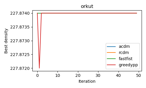
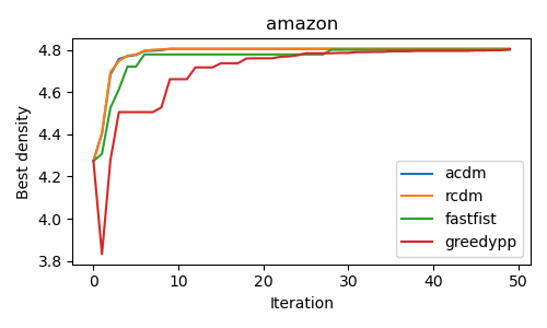
(a) Iteration/Best Density

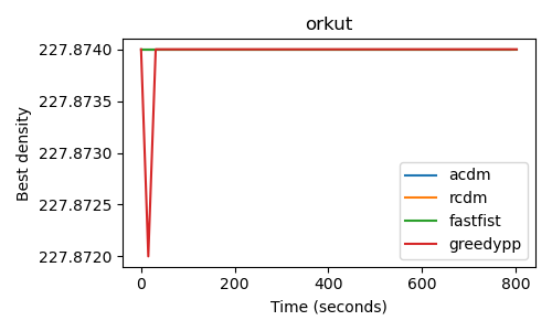
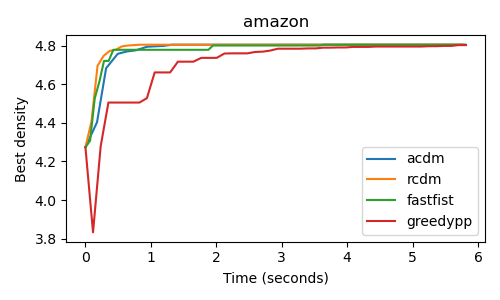
(b) Time/Best Density

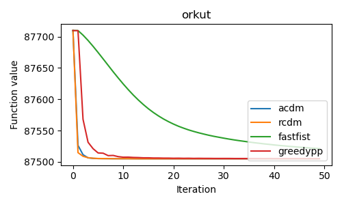
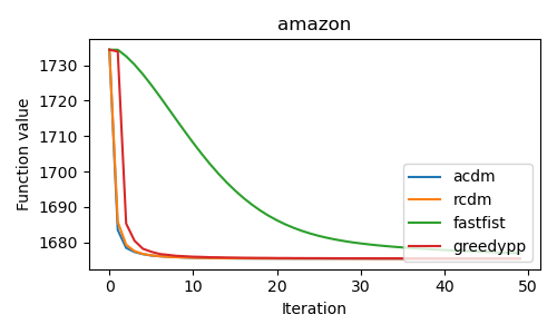
(c) Iteration/Load norm $\left(\sum_{u\in V}b_{u}^{2}\right)^{1/2}$

Figure 1: Experiment results on orkut and com-Amazon. In the legends: acdm, rcdm, fastfist, greedypp respectively represent Algorithm 5, Algorithm 7, FISTA-based algorithm by Harb et al. (2022) and Greedy++ (Boob et al., 2020)

In this section, we compare the performance of existing algorithms and Algorithm 5. We also consider the version of Algorithm 5 without acceleration, Algorithm 7 shown in the appendix. On the other hand, due to the involved subroutines, we do not compare the performance of Algorithm 1 and 3. We follow the experimental set up in prior works, including Boob et al. (2020) and Harb et al. (2022).

Benchmark.   We consider three algorithms: Frank-Wolfe (Danisch et al., 2017), implemented by Harb et al. (2022), Greedy++ (Boob et al., 2020) and FISTA for DSG (Harb et al., 2022).

Implementation.   We use the implementation of all benchmark algorithms provided by Harb et al. (2022). The implementation of our algorithms also uses the same code base by Harb et al. (2022). For practical purposes, we modify Algorithms 5 and 7 by replacing the inner loop with making passes over random permutations of the edges instead of random sampling edges. We also restart Algorithm 5 after each pass that increases the function value. We show the pseudocode for these variants in Algorithms 6 in the appendix and in Option 2 of Algorithm 7. For all algorithms, we initialize at the solution by the Greedy peeling algorithm (Charikar, 2000).

Datasets.   The algorithms are compared on eight different datasets, summarized in Table 2 (appendix).

For a fair comparison, for all algorithms considered, we define an iteration as a run of $m$ edge updates, and each update can be implemented in a constant time.

We plot the best density obtained by each algorithm over the iterations in Figure 1a. In Figure 1b, we plot the best density over wall clock time. Finally, Figure 1c shows the function value ($L_{2}$-norm of the load vector) $\left(\sum_{u\in V}b_{u}^{2}\right)^{1/2}$ over the iterations. Due to space limit, we only show plots for two datasets: com-Amazon and orkut. We also exclude Frank-Wolfe in the plots due to its significantly worse performance in all instances. We defer the remaining plots and plots that include Frank-Wolfe to the appendix.

Discussion.    We can observe that Algorithms 5 and 7 are practical and can run on relatively fast large instances (for example, orkut has more than $3$ million vertices and $100$ million edges). Figure 1c shows that both Algorithms 5 and 7 outperform the others at minimizing the function value. Especially in comparison with FISTA, both Algorithms 5 and 7 are significantly better.

Boob et al. (2020) observed that in most instances, the Greedy peeling algorithm by Charikar (2000) already finds a near-optimal densest subgraph. Greedy++ inherits this feature of Greedy and generally has a very good performance across instances. Algorithms 5 and 7 with initialization by the Greedy algorithm have competitive performances with Greedy++ and FISTA both in terms of the number of iterations and time.

7 Conclusion

In this paper, we present several algorithms for the DSG problems. We show new algorithms via multiplicative weights update and area convexity with improved running times. We also give the first practical algorithm with a linear convergence rate via random coordinate descent. Obtaining a practical implementation of our multiplicative weights update algorithm in the streaming and distributed settings, and using our results to improve algorithms for DSG problems in other settings such as differential privacy are among potential future works.

Appendix A Additional Proofs from Section 3

A.1 Multiplicative Weights Update analysis tool: $\mathrm{smax}$ function

We analyze our MWU algorithm via the $\mathrm{smax}$ function, defined as follows. For $x\in\mathbb{R}^{n}$ and $\eta\in\mathbb{R}_{+}$, we define

$$\mathrm{smax}_{\eta}(x)=\frac{1}{\eta}\ln\left(\sum_{i=1}^{n}\exp\left(\eta x_{i}\right)\right).$$

$\mathrm{smax}_{\eta}(x)$ can be seen as a smooth approximation of $\max(x)\overset{\mathrm{def}}{=}\max_{i}x_{i}\leq\max_{i}\left|x_{i}\right|=\left\|x\right\|_{\infty}$, in the following sense

$$\left\|x\right\|_{\infty} \leq\mathrm{smax}_{\eta}(x)\leq\frac{\ln n}{\eta}+\left\|x\right\|_{\infty},$$

and $\mathrm{smax}_{\eta}$ is $\eta$-smooth with respect to $\left\|\cdot\right\|_{\infty}$: $\forall x,u,$

$$\mathrm{smax}_{\eta}(x+u)\leq\mathrm{smax}_{\eta}(x)+\left\langle\nabla\mathrm{smax}_{\eta}(x),u\right\rangle+\text{$\frac{\eta}{2}$}\left\|u\right\|_{\infty}^{2}.$$

The gradient of $\mathrm{smax}_{\eta}$ is a probability distribution in $\Delta_{n}=\left\{p\in\mathbb{R}_{\geq 0}^{n}\colon p_{1}+\dots+p_{n}=1\right\}$:

$$\left(\nabla\mathrm{smax}_{\eta}(x)\right)_{i}=\text{$\frac{\exp(\eta x_{i})}{\sum_{j}\exp(\eta x_{j})}$}.$$

A.2 Proof of Lemma 3.1

Proof.

Note that $z^{*}$ can be decreased so that $z_{eu}^{*}+z_{ev}^{*}=1,\ \forall e=uv\in E$, without increasing the objective. Hence, we can have $\sum_{e\in E}p_{e}^{(t)}\left(z_{eu}^{*}+z_{ev}^{*}\right)=\sum_{e\in E}p_{e}^{(t)}=1$. This means $z^{*}$ satisfies the constraint of LP (5), thus for all $t$, since $z^{(t)}$ is an optimal solution to (5) with $p^{(t)}$, we have

$$\max_{v\in V}\sum_{e\in E,u\in e}z_{eu}^{(t)} \leq\max_{v\in V}\sum_{e\in E,u\in e}z_{eu}^{*},$$

which implies

$$\max_{v\in V}\sum_{e\in E,u\in e}\overline{z}_{eu} =\max_{v\in V}\frac{1}{T}\sum_{t=1}^{T}\sum_{e\in E,u\in e}z_{eu}^{(t)}$$

$$\leq\frac{1}{T}\sum_{t=1}^{T}\max_{v\in V}\sum_{e\in E,u\in e}z_{eu}^{(t)}$$

$$\leq\max_{v\in V}\sum_{e\in E,u\in e}z_{eu}^{*}.$$

Moreover, since $\mathrm{smax}_{\eta}$ is $\eta$-smooth wrt $\left\|\cdot\right\|_{\infty}$, we have

$$\mathrm{smax}_{\eta}(G^{(t)})-\mathrm{smax}_{\eta}(G^{(t-1)}) \leq\left\langle\nabla\mathrm{smax}_{\eta}(G^{(t-1)}),g^{(t)}\right\rangle+\frac{\eta}{2}\left\|g^{(t)}\right\|_{\infty}^{2}$$

$$=\sum_{e\in E}p_{e}^{(t)}\left(1-\left(z_{eu}^{(t)}+z_{ev}^{(t)}\right)\right)+\frac{\eta}{2}\left\|g^{(t)}\right\|_{\infty}^{2}$$

$$=\frac{\eta}{2}\left\|g^{(t)}\right\|_{\infty}^{2},$$

where we use $g^{(t)}=1-\left(z_{eu}^{(t)}+z_{ev}^{(t)}\right)$ and $\nabla\mathrm{smax}_{\eta}(G^{(t-1)})=p^{(t)}$. Note that $g_{e}^{(t)}=1-\left(z_{eu}^{(t)}+z_{ev}^{(t)}\right)\in\left[-1,1\right].$Thus

$$\mathrm{smax}_{\eta}(G^{(T)}) \leq\underbrace{\mathrm{smax}_{\eta}(G^{(0)})}_{=\frac{\ln m}{\eta}}+\sum_{t=1}^{T}\frac{\eta}{2}\underbrace{\left\|g^{(t)}\right\|_{\infty}^{2}}_{\leq 1}\leq\frac{\ln m}{\eta}+\frac{\eta}{2}T.$$

Thus we have

$$\max\left(G^{(T)}\right)\leq\mathrm{smax}_{\eta}(G^{(T)})\leq\frac{\ln m}{\eta}+\frac{\eta}{2}T$$

and hence

$$\max\left(\left(1-\left(\overline{z}_{eu}+\overline{z}_{ev}\right)\right)_{e\in E}\right)\leq\frac{1}{T}\frac{\ln m}{\eta}+\frac{\eta}{2}.$$

By the choice $\eta=\epsilon$ and $T=\frac{2\ln m}{\epsilon\eta}=\frac{2\ln m}{\epsilon^{2}}$, we obtain $\frac{1}{T}\frac{\ln m}{\eta}+\frac{\eta}{2}\leq\epsilon$, i.e.,

$$1-\left(\overline{z}_{eu}+\overline{z}_{ev}\right)\leq\epsilon\quad\forall e=uv.$$

∎

A.3 Proof of Corollary 3.2

Proof.

Assume the contradiction: for all $t\in[T]$ we have $D^{(t)}<\left(1-\epsilon\right)D^{*},$ which means $\max_{v\in V}\sum_{e\in E,u\in e}z_{eu}^{(t)}<\left(1-\epsilon\right)D^{*}.$ Then

$$\max_{v\in V}\sum_{e\in E,u\in e}\overline{z}_{eu} =\max_{v\in V}\frac{1}{T}\sum_{t=1}^{T}\sum_{e\in E,u\in e}z_{eu}^{(t)}$$

$$\leq\frac{1}{T}\sum_{t=1}^{T}\max_{v\in V}\sum_{e\in E,u\in e}z_{eu}^{(t)}$$

$$<\left(1-\epsilon\right)D^{*}.$$

On the other hand, we have for all $e=uv$, $\overline{z}_{eu}+\overline{z}_{ev}\geq 1-\epsilon$. We let $\widetilde{z}_{eu}=\frac{\overline{z}_{eu}}{\overline{z}_{eu}+\overline{z}_{ev}}$. In this way we have $\widetilde{z}_{eu}+\widetilde{z}_{ev}=1$ and $\widetilde{z}_{eu}\leq\frac{\overline{z}_{eu}}{1-\epsilon}$. Therefore $\widetilde{z}$ satisfies the constraint of (3). Furthermore

$$\max_{v\in V}\sum_{e\in E,u\in e}\widetilde{z}_{eu} \leq\frac{1}{1-\epsilon}\max_{v\in V}\sum_{e\in E,u\in e}\overline{z}_{eu}<D^{*}.$$

which means $\widetilde{z}$ has a better objective than $z^{*}$, contradiction. ∎

A.4 Proof of Lemma 3.3

Proof.

First, $z^{*}$ satisfies $\sum_{e\in E,u\in e}z_{eu}^{*}\leq D^{*}$ for all $u$. Assume that $\widetilde{z}$ is an optimal solution to (5). For each $u$ we show that

$$\sum_{e\in E,u\in e}p_{e}z_{eu}^{*} \geq\sum_{e\in E,u\in e}p_{e}\widetilde{z}_{eu}.$$ (16)

Indeed, if $\deg u\leq\lfloor D^{*}\rfloor$ we have $z_{eu}^{*}=1$ for all $e\ni u$. Hence (16) holds. Otherwise we have

$$\sum_{e\in E,u\in e}z_{eu}^{*} =D^{*}\geq\sum_{e\in E,u\in e}\widetilde{z}_{eu}.$$

Furthermore $z^{*}$ satisfies $z_{eu}^{*}\geq z_{e^{\prime}u}^{*}$ if $p_{e}\geq p_{e^{\prime}}$, hence $\sum_{e\in E,u\in e}p_{e}z_{eu}^{*}$ maximizes $\sum_{e\in E,u\in e}p_{e}z_{eu}$ subject to $\sum_{e\in E,u\in e}z_{eu}\leq D^{*}$. Thus (16) holds. Therefore

$$\sum_{u\in V}\sum_{e\in E,u\in e}p_{e}z_{eu}^{*} \geq\sum_{u\in V}\sum_{e\in E,u\in e}p_{e}\widetilde{z}_{eu}=1.$$

If $\sum_{u\in V}\sum_{e\in E,u\in e}p_{e}z_{eu}^{*}>1$, we can decrease the value of $z$ for all the vertices where $\sum_{e\in E,u\in e}z_{eu}^{*}=D^{*}$ thus obtains a solution with strictly better objective than $D^{*}$, which is a contradiction. Therefore $z^{*}$ is an optimal solution. ∎

A.5 Proof of Lemma 3.5

Proof.

We verify by complementary slackness.

1) We have$\sum_{v}x_{v}=1$.

2) $\sum_{e\ni u}z_{eu}^{(\tau)}<D^{(\tau)}\Leftrightarrow u\notin X\Leftrightarrow x_{u}=0$.

3) For all $u\notin X$ we have $z_{eu}^{(\tau)}=1$ for all $e\ni u$ and $\alpha_{eu}=p_{e}^{(\tau)}W$. For $u\in X$ such that $z_{eu}^{(\tau)}=0$, we have $p_{e}^{(\tau)}\leq p_{e(u)}^{(\tau)}$, so $\alpha_{eu}=0$. For $u\in X$, $z_{eu}^{(\tau)}=z_{e(u)u}^{(\tau)}$, we have also $\alpha_{eu}^{(\tau)}=0$. For $u\in X$ such that $z_{eu}^{(\tau)}>0$, we also guarantee $p_{e}^{(\tau)}W+\alpha_{eu}^{(\tau)}=x_{u}$. $p_{e}^{(\tau)}W<x_{u}+\alpha_{eu}$ happens only when $p_{e}^{(\tau)}<p_{e(u)}^{(\tau)}$ which gives $z_{eu}=0$. ∎

A.6 Proof of Lemma 3.6

Proof.

By strong duality we have

$$W-\sum_{e=uv}\left(\alpha_{eu}+\alpha_{ev}\right) =D^{(\tau)}.$$

We know that $D^{(\tau)}\geq\left(1-\epsilon\right)D^{*}=\left(1-\epsilon\right)\mathrm{OPT}$. Hence $\sum_{e}\left(p_{e}^{(\tau)}W-\left(\alpha_{eu}+\alpha_{ev}\right)\right)=W-\sum_{e=uv}\left(\alpha_{eu}+\alpha_{ev}\right)\geq\left(1-\epsilon\right)\mathrm{OPT}.$ On the other hand, since

$$p_{e}^{(\tau)}W-\left(\alpha_{eu}+\alpha_{ev}\right) \leq p_{e}^{(\tau)}W-\alpha_{eu}\leq x_{u},$$

$$p_{e}^{(\tau)}W-\left(\alpha_{eu}+\alpha_{ev}\right) \leq p_{e}^{(\tau)}W-\alpha_{ev}\leq x_{v}.$$

We have $\sum_{e=uv}\min\{x_{u},x_{v}\}\geq\sum_{e=uv}(p_{e}^{(\tau)}W-(\alpha_{eu}+\alpha_{ev}))\geq(1-\epsilon)\mathrm{OPT},$ as needed. ∎

Appendix B Additional Proofs from Section 4

B.1 Area convexity functions review

We first review the notion of area convexity introduced by Sherman (2017).

Definition B.1.

A function $\phi$ is area convex with respect to an anti-symmetric matrix $A$ on a convex set $K$ if for every $x,y,z\in K$,

$$\phi\left(\frac{x+y+z}{3}\right) \leq\frac{1}{3}\left(\phi\left(x\right)+\phi\left(y\right)+\phi\left(z\right)\right)-\frac{1}{3\sqrt{3}}\left(x-y\right)^{T}A\left(y-z\right).$$

To show that a function is area convex, Boob et al. (2019) employ operator $\succeq_{i}$. For a symmetric matrix $A$ and an anti-symmetric matrix $B$, we say $A\succeq_{i}B$ iff $\left[\begin{array}[]{cc}A&-B^{T}\\ B&A\end{array}\right]$ is PSD. The following two lemmas are from Boob et al. (2019).

Lemma B.2.

(Lemma 4.5 in Boob et al. (2019)) Let $A$ be a $\mathbb{R}^{2\times 2}$ symmetric matrix. $A\succeq_{i}\left[\begin{array}[]{cc}0&-1\\ 1&0\end{array}\right]$ iff $A\succeq 0$ and $\det A\geq 1$.

Lemma B.3.

(Lemma 4.6 in Boob et al. (2019)) Let $\phi$ be twice differentiable on the interior of convex set $K$, i.e $\mathrm{int}(K)$. If $\nabla^{2}\phi(x)\succeq_{i}A$ for all $x\in\mathrm{int}(K)$ then $\phi$ is area convex with respect to $\frac{1}{3}A$ on $\mathrm{int}(K)$. If moreover, $\phi$ is continuous on $\mathrm{cl}(K)$ then $\phi$ is area convex with respect to $\frac{1}{3}A$ on $\mathrm{cl}(K)$.

B.2 Reduction to the saddle point problem

Lemma B.4.

(Lemma 4.3 in Boob et al. (2019)) Suppose $z\in C,y\in\Delta_{m}$ satisfy

$$\max_{\overline{z}\in C,\overline{y}\in\Delta_{m}}\sum_{e}y_{e}\left(\overline{z}_{eu}+\overline{z}_{ev}\right)-\overline{y}_{e}\left(z_{eu}+z_{ev}\right) \leq\epsilon,$$

then either of the following happens:

1. $z$ is an $\epsilon$-approximate solution to the feasibility problem,

2. $y$ satisfies for all $\overline{z}\in C$, $\sum_{e}y_{e}\left(\overline{z}_{eu}+\overline{z}_{ev}\right)<1$.

Proof.

Suppose that $z$ is not an $\epsilon$-approximate solution to the problem. This means there exists $e=uv$ such that $z_{eu}+z_{ev}<1-\epsilon$, which implies

$$\min_{\overline{y}\in\Delta_{m}}\overline{y}_{e}\left(z_{eu}+z_{ev}\right) <1-\epsilon$$

Since

$$\max_{\overline{z}\in C,\overline{y}\in\Delta_{m}}\sum_{e}y_{e}\left(\overline{z}_{eu}+\overline{z}_{ev}\right)-\overline{y}_{e}\left(z_{eu}+z_{ev}\right)$$

$$= \max_{\overline{z}\in C}\sum_{e}y_{e}\left(\overline{z}_{eu}+\overline{z}_{ev}\right)-\min_{\overline{y}\in\Delta_{m}}\overline{y}_{e}\left(z_{eu}+z_{ev}\right)\leq\epsilon,$$

we can conclude that

$$\max_{\overline{z}\in C}\sum_{e}y_{e}\left(\overline{z}_{eu}+\overline{z}_{ev}\right) <1.$$

∎

B.3 Properties of the regularizer

We recall the choice of the regularizer function

$$\phi(z,y) =6\sqrt{3}\left(\sum_{e\in E}y_{e}\left(z_{eu}^{2}+z_{ev}^{2}\right)+6y_{e}\log y_{e}-2\right).$$

Our goal is to show that $\phi$ is area convex with respect to $A$ and has a small range.

Lemma B.5.

$\frac{1}{6\sqrt{3}}\phi$ is area convex with respect to $\frac{1}{3}A$. Furthermore $-6\sqrt{3}\left(6\log m+2\right)\leq\phi(z,y)\leq 0$.

Proof.

By Lemma B.3, it suffices to show that

$$\nabla^{2}\phi(z,y) \succeq_{i}A.$$

Let $\vec{f}_{e}$ denote the vector with all $0$’s and one $1$ at the index of $y_{e}$, $\vec{f}_{eu}$ denote the vector with all $0$’s and one $1$ at the index of $z_{ev}$ and $\vec{f}_{u}$ for $u$. Consider two variables $y_{e}$ and $z_{eu}$, we have

$$\nabla^{2}y_{e}\left(\left(z_{eu}^{2}+3\log y_{e}\right)\right) =\left[\begin{array}[]{cc}\frac{3}{y_{e}}&2z_{eu}\\ 2z_{eu}&2y_{e}\end{array}\right]\succeq_{i}\left[\begin{array}[]{cc}0&-1\\ 1&0\end{array}\right]$$

where the last inequality comes from Lemma B.2 and that

$$\det\left[\begin{array}[]{cc}\frac{3}{y_{e}}&2z_{eu}\\ 2z_{eu}&2y_{e}\end{array}\right] =6-4z_{eu}^{2}>1,$$

which holds because $0\leq z_{eu}\leq 1$. By Lemma 4.10 in Boob et al. (2019)

$$\nabla^{2}y_{e}\left(\left(z_{eu}^{2}+3\log y_{e}\right)+\left(z_{ev}^{2}+3\log y_{e}\right)\right)$$

$$\succeq_{i} \left(\vec{f}_{e}\vec{f}_{eu}^{T}-\vec{f}_{eu}\vec{f}_{e}^{T}\right)+\left(\vec{f}_{e}\vec{f}_{ev}^{T}-\vec{f}_{ev}\vec{f}_{e}^{T}\right).$$

Sum up the RHS we get exactly $A.$

For the lower bound

$$\frac{1}{6\sqrt{3}}\phi(z,y)=\sum_{e}y_{e}\left(z_{eu}^{2}+z_{ev}^{2}\right)+6\sum_{e}y_{e}\log y_{e}-2$$

$$\geq 6\underbrace{\sum_{e}y_{e}\log y_{e}}_{\mbox{convexity}}-2\geq 6m\frac{1}{m}\log\frac{1}{m}-2=-6\log m-2.$$

For the upper bound

$$\frac{1}{6\sqrt{3}}\phi(z,y) \leq 2\sum_{e}y_{e}-2=0.$$

∎

B.4 Proof of Lemma 4.2

Proof.

The proof of this Lemma directly follows from Theorem 1.3 in Sherman (2017) and that

$$\phi^{*}(w^{(0)}) =\sup_{w\in C\times\Delta_{m}}\left\langle w,w^{(0)}\right\rangle-\phi(w)$$

$$=\sup_{w\in C\times\Delta_{m}}1-\phi(w)$$

$$\leq 1+6\sqrt{3}\left(6\log m+2\right).$$

∎

B.5 Proof of Lemma 4.3

Proof.

The proof of Lemma 4.3 follows from the general framework for analyzing alternating minimization by Beck (2015). The proof detail below follows from Jambulapati et al. (2019).

For simplicity, let us recall the definition of $H$ in Algorithm 4, after scaling by $\frac{1}{6\sqrt{3}}$. Given $x=(s,r)$ is the input, we have

$$H(z,y)\coloneqq \sum_{e=uv\in E}y_{e}\left(z_{eu}^{2}+z_{ev}^{2}\right)+6\sum_{e}y_{e}\log y_{e}$$

$$-\frac{1}{6\sqrt{3}}\Big{(}\sum_{e=uv\in E}(z_{eu}s_{eu}+z_{ev}s_{ev}+y_{e}r_{e})\Big{)}.$$

Let $\nabla_{zz}^{2}$ be the Hessian with all but the $zz$ block zeroed out. We use $\nabla_{y}$ and $\nabla_{z}$ to denote the gradient with only the $y$ and $z$ components kept.

Let $Y^{(t+1)}=\left\{y\in\Delta_{m}:y\geq\frac{1}{2}y^{(t+1)}\right\}$. We will first show that for all $z,\overline{z}\in C$ and $\overline{y}\in Y^{(t+1)}$

$$\nabla^{2}H(\overline{z},\overline{y}) \succeq\frac{1}{6}\nabla_{zz}^{2}H(z,y^{(t+1)})$$ (17)

Since we do not have any cross term between $e$ and $e^{\prime}$ for any $e\neq e^{\prime}$ we can consider edge separately. For the same reason, we can also separate $z_{eu}$ and $z_{ev}$ for each edge $e$. The non-zero term after taking the Hessian for edge $e$ and vertex $u$ is

$$\nabla^{2}\overline{y}_{e}\left(\left(\overline{z}_{eu}^{2}+3\log\overline{y}_{e}\right)\right) =\left[\begin{array}[]{cc}\frac{3}{\overline{y}_{e}}&2\overline{z}_{eu}\\ 2\overline{z}_{eu}&2\overline{y}_{e}\end{array}\right];$$

$$\nabla_{zz}^{2}y_{e}^{(t+1)}\left(\left(z_{eu}^{2}+3\log y_{e}^{(t+1)}\right)\right) =\left[\begin{array}[]{cc}0&0\\ 0&2y_{e}^{(t+1)}\end{array}\right].$$

For all $a,b\in\mathbb{R}$

$$\left[\begin{array}[]{cc}a&b\end{array}\right]\nabla^{2}\overline{y}_{e}\left(\left(\overline{z}_{eu}^{2}+3\log\overline{y}_{e}\right)\right)\left[\begin{array}[]{c}a\\ b\end{array}\right]= \frac{3}{\overline{y}_{e}}a^{2}+2\overline{y}_{e}b^{2}+4\overline{z}_{eu}ab;$$

$$\left[\begin{array}[]{cc}a&b\end{array}\right]\nabla_{zz}^{2}y_{e}^{(t+1)}\left(\left(z_{eu}^{2}+3\log y_{e}^{(t+1)}\right)\right)\left[\begin{array}[]{c}a\\ b\end{array}\right]= 2y_{e}^{(t+1)}b^{2}.$$

Since $z_{eu},\overline{z}_{eu}\leq 1$

$$\frac{3}{\overline{y}_{e}}a^{2}+2\overline{y}_{e}b^{2}+4\overline{z}_{eu}ab \geq\frac{3}{\overline{y}_{e}}a^{2}+2\overline{y}_{e}b^{2}-4\left|ab\right|$$

$$\geq\frac{2}{3}\overline{y}_{e}b^{2}$$

$$\geq\frac{1}{3}y_{e}^{(t+1)}b^{2}\mbox{ for all }y\geq\frac{1}{2}y^{(t+1)}$$

$$=\frac{1}{6}\times 2y_{e}^{(t+1)}b^{2}.$$

Hence for all $y\geq\frac{1}{2}y^{(t+1)}$

$$\nabla^{2}\overline{y}_{e}\left(\overline{z}_{eu}^{2}+3\log\overline{y}_{e}\right) \succeq\nabla_{zz}^{2}y_{e}^{(t+1)}\left(z_{eu}^{2}+3\log y_{e}^{(t+1)}\right)$$

which gives us (17).

Now we show that or all $y^{*}\in Y^{(t+1)}$ and $z^{*}\in C$

$$H(z^{(t)},y^{(t+1)})-H(z^{(t+1)},y^{(t+1)}) \geq\frac{1}{6}\left(H(z^{(t)},y^{(t+1)})-H(z^{*},y^{*})\right).$$

Let $\tilde{z}=\frac{5}{6}z^{(t)}+\frac{1}{6}z^{*}$. By the definition of $z^{(t+1)}$ we have

$$H(z^{(t+1)},y^{(t+1)}) \leq H(\tilde{z},y^{(t+1)}.)$$

By the optimality of $y^{(t+1)}$ and the convexity of $H$

$$\left\langle\nabla_{y}H(z^{(t)},y^{(t+1)}),y^{(t+1)}-y^{*}\right\rangle \leq 0$$

which gives us

$$\left\langle\nabla_{z}H(z^{(t)},y^{(t+1)}),z^{(t)}-\tilde{z}\right\rangle= \frac{1}{6}\left\langle\nabla_{z}H(z^{(t)},y^{(t+1)}),z^{(t)}-z^{*}\right\rangle$$

$$\geq \frac{1}{6}\left\langle\nabla_{z}H(z^{(t)},y^{(t+1)}),z^{(t)}-z^{*}\right\rangle$$

$$+\frac{1}{6}\left\langle\nabla_{y}H(z^{(t)},y^{(t+1)}),y^{(t+1)}-y^{*}\right\rangle$$

$$= \frac{1}{6}\left\langle\nabla H(z^{(t)},y^{(t+1)}),w^{(t+\frac{1}{2})}-w^{*}\right\rangle$$

where $w^{(t+\frac{1}{2})}=(z^{(t)},y^{(t+1)})$, $w^{*}=(z^{*},y^{*})$. Also define $z_{\alpha}=\left(1-\alpha\right)z^{(t)}+\alpha z^{*}$, $\tilde{z}_{\alpha}=\left(1-\alpha\right)z^{(t)}+\alpha\tilde{z}$, $y_{\alpha}=\left(1-\alpha\right)y^{(t+1)}+\alpha y^{*}$. With a slight abuse of notion, we also use $\nabla_{zz}^{2}$ to also mean the Hessian with respect to the variable $z$. Using Taylor expansion

$$H(z^{(t)},y^{(t+1)})-H(\tilde{z},y^{(t+1)})= \left\langle\nabla_{z}H(z^{(t)},y^{(t+1)}),z^{(t)}-\tilde{z}\right\rangle$$

$$-\int_{0}^{1}\int_{0}^{\beta}\left(\tilde{z}-z^{(t)}\right)^{T}\nabla_{zz}^{2}H(\tilde{z}_{\alpha},y^{(t+1)})\left(\tilde{z}-z^{(t)}\right)d\alpha d\beta$$

$$\geq \frac{1}{6}\left\langle\nabla H(z^{(t)},y^{(t+1)}),w^{(t+\frac{1}{2})}-w^{*}\right\rangle$$

$$-\frac{1}{36}\int_{0}^{1}\int_{0}^{\beta}\left(z^{*}-z^{(t)}\right)^{T}\nabla_{zz}^{2}H(\tilde{z}_{\alpha},y^{(t+1)})\left(z^{*}-z^{(t)}\right)d\alpha d\beta$$

$$\geq \frac{1}{6}\left\langle\nabla H(z^{(t)},y^{(t+1)}),w^{(t+\frac{1}{2})}-w^{*}\right\rangle$$

$$-\frac{1}{6}\int_{0}^{1}\int_{0}^{\beta}\left(w^{*}-w^{(t+\frac{1}{2})}\right)^{T}\nabla^{2}H(z_{\alpha},y_{\alpha})\left(w^{*}-w^{(t+\frac{1}{2})}\right)d\alpha d\beta$$

$$=\frac{1}{6}\left(H(z^{(t)},y^{(t+1)})-H(z^{*},y^{*})\right).$$

Hence

$$H(z^{(t)},y^{(t+1)})-H(z^{(t+1)},y^{(t+1)})\geq H(z^{(t)},y^{(t+1)})-H(\tilde{z},y^{(t+1)})$$

$$\geq \frac{1}{6}\left(H(z^{(t)},y^{(t+1)})-H(z^{*},y^{*})\right).$$

Take $z^{*}=\frac{1}{2}\left(z^{(t)}+z_{\mathrm{OPT}}\right)$, $y^{*}=\frac{1}{2}\left(y^{(t+1)}+y_{\mathrm{OPT}}\right)$

$$H(z^{(t)},y^{(t+1)})-H(z^{(t+1)},y^{(t+2)})\geq H(z^{(t)},y^{(t+1)})-H(z^{(t+1)},y^{(t+1)})$$

$$\geq \frac{1}{6}\left(H(z^{(t)},y^{(t+1)})-H(z^{*},y^{*})\right)$$

$$\geq \frac{1}{6}\left(H(z^{(t)},y^{(t+1)})-\left(\frac{1}{2}H(z^{(t)},y^{(t+1)})+\frac{1}{2}H\left(z_{\mathrm{OPT}},y_{\mathrm{OPT}}\right)\right)\right)$$

$$\qquad\qquad(\mbox{by convexity of }H)$$

$$= \frac{1}{12}\left(H(z^{(t)},y^{(t+1)})-H\left(z_{\mathrm{OPT}},y_{\mathrm{OPT}}\right)\right)$$

which means

$$H(z^{(t+1)},y^{(t+2)})-H\left(z_{\mathrm{OPT}},y_{\mathrm{OPT}}\right) \leq\frac{11}{12}\left(H(z^{(t)},y^{(t+1)})-H\left(z_{\mathrm{OPT}},y_{\mathrm{OPT}}\right)\right).$$

Therefore

$$H(z^{(T+1)},y^{(T+1)})-H\left(z_{\mathrm{OPT}},y_{\mathrm{OPT}}\right) \leq\left(\frac{11}{12}\right)^{T}\left(H(z^{(0)},y^{(1)})-H\left(z_{\mathrm{OPT}},y_{\mathrm{OPT}}\right)\right).$$

This gives us the convergence rate. ∎

B.6 Proof of Lemma 4.4

Proof.

For the first minimization, we have $y^{(t+1)}=\arg\min_{y\in\Delta_{m}}H(z^{(t)},y)=\arg\max_{y\in\Delta_{m}}\left\langle L^{(t)},y\right\rangle-\sum_{e}y_{e}\log y_{e}$, where $L_{e}^{(t)}=-\frac{1}{6}\left(\left(z_{eu}^{(t)2}+z_{ev}^{(t)2}\right)-\frac{1}{6\sqrt{3}}r_{e}\right)$. The solution is simply $\nabla\mathrm{smax}(L^{(t)})$ (definition in Section A.1), which can be computed in $O(m)$.

The second minimization $z^{(t+1)}=\arg\min_{z\in C}H(z,y^{(t+1)})$. Here we build on the insights from the oracle implementation for MWU and reduce the problem to computing for each $u$ separately

$$\min_{z\in[0,1]^{\deg(u)}} \sum_{e\ni u}z_{eu}^{2}y_{e}^{(t+1)}-\frac{1}{6\sqrt{3}}z_{eu}s_{eu}\mbox{ st. }\sum_{e\ni u}z_{eu}\leq D$$

Let $\tilde{s}=\frac{1}{6\sqrt{3}}s$ and take the Lagrangian, we have

$$\min_{z\in[0,1]^{\deg(u)}}\max_{\lambda\geq 0} \sum_{e\ni u}\left(z_{eu}^{2}y_{e}^{(t+1)}-z_{eu}\tilde{s}_{eu}+\lambda z_{eu}\right)-\lambda D$$

$$\Leftrightarrow\max_{\lambda\geq 0}\min_{z\in[0,1]^{\deg(u)}} \sum_{e\ni u}\left(z_{eu}^{2}y_{e}^{(t+1)}-z_{eu}\tilde{s}_{eu}+\lambda z_{eu}\right)-\lambda D$$

For $\lambda\geq 0$, we obtain for each $e\ni u$

$$z_{eu} =\max\left\{0,\min\left\{1,\frac{\tilde{s}_{eu}-\lambda}{2y_{e}^{(t+1)}}\right\}\right\}$$

Now we need to solve for $\lambda$

$$\max_{\lambda\geq 0}\sum_{e\ni u}\left(z_{eu}^{2}y_{e}^{(t+1)}-z_{eu}\tilde{s}_{eu}+\lambda z_{eu}\right)-\lambda D$$

$$= \max_{\lambda\geq 0}-\lambda D+\sum_{z:0\leq\tilde{s}_{eu}-\lambda\leq 2y_{e}^{(t+1)}}-\frac{\left(\tilde{s}_{eu}-\lambda\right)^{2}}{4y_{e}^{(t+1)}}$$

$$\quad+\sum_{z:\tilde{s}_{eu}-\lambda>2y_{e}^{(t+1)}}\left(y_{e}^{(t+1)}-\tilde{s}_{eu}+\lambda\right).$$

Again, we take the inspiration from Algorithm 2 and see that we can also perform a search for $\lambda$. Here each $e\ni u$ belongs to one of the three category, $\tilde{s}_{eu}-\lambda<0$ or $0\leq\tilde{s}_{eu}-\lambda\leq 2y_{e}^{(t+1)}$ or $\tilde{s}_{eu}-\lambda>2y_{e}^{(t+1)}$. To solve the above problem, we must determine which category each $e$ belongs to. To do this, we can sort 2$\deg u$ numbers $\left\{\max\left\{2y_{e}^{(t+1)}-\tilde{s}_{eu},0\right\},\tilde{s}_{eu}\right\}_{e\ni u}$ and find the optimal value of $\lambda$ on each interval. When testing $\lambda$ increasingly, the category of each $z_{eu}$ only changes at most twice. For this we can use a data structure (eg. Fibonacci heap) to determine which $z_{eu}$ changes category when $\lambda$ jumps to the next interval. This means the total time to find $z_{eu}$ for all $e\ni u$ is at most $O(\deg u\log\deg u)$. Summing the total over all vertex $u$, we have solving the second minimization problem each iteration takes $O(m\log\Delta)$ time. ∎

B.7 Proof of Lemma 4.6

Proof.

Observe that the following LP is infeasible for $z\in[0,1]^{2m}$

$$\sum_{e\ni u}z_{eu} \leq\overline{D},\quad\forall u\in V$$

$$z_{eu}+z_{ev} \geq 1-\epsilon\quad\forall e=uv\in E.$$

Because otherwise, similar to lemma 3.2, we must have $\overline{D}\geq D^{*}(1-\epsilon)$, while we have $\overline{D}=\tilde{D}(1-2\epsilon)\leq D^{*}(1+\epsilon)(1-2\epsilon)<D^{*}(1-\epsilon)$, contradiction. Thus we have that

$$\max_{z\in C(\overline{D})}\sum_{e}\overline{y}_{e}\left(z_{eu}+z_{ev}\right)\leq \epsilon+\min_{y\in\Delta_{m}}\sum_{e}y_{e}\left(\overline{z}_{eu}+\overline{z}_{ev}\right)<\epsilon+1-\epsilon=1.$$

This gives us the claim in the lemma. ∎

Appendix C Additional Proofs from Section 5

C.1 Continuous formulation

We recall with the quadratic program for finding a dense decomposition

$$\min f(z)\coloneqq\sum_{u\in V}b_{u}^{2}\mbox{ st. } b_{u}=\sum_{e\in E,u\in e}z_{eu},\quad\forall u\in V$$ (18)

$$z_{eu}+z_{ev}\geq 1,\quad\forall e=uv\in E$$

$$0\leq z_{eu}\leq 1,\quad\forall e,u\in e\in E.$$

Now, we show how to reformulate this problem as (15). Recall that we define for $e\in E$, $F_{e}(S)=1$ if $e\subseteq S$, $F_{e}(S)=0$ otherwise and the base contrapolymatroid

$$B(F_{e}) =\left\{z_{e}\in\mathbb{R}^{n},z_{e}(S)\geq F_{e}(S)\;\forall S\subseteq V,z_{e}(V)=F_{e}(V)=1\right\}$$

Specifically, for $z_{e}\in B(F_{e})$, we have

$$z_{eu}+z_{ev} =1,\quad\mbox{for }e=uv$$

$$z_{ew} =0,\quad\forall w\neq u,v$$

In this view, it is immediate to see that we can rewrite the above problem as

$$\min_{z_{e}\in B(F_{e}),\forall e\in E} \left\|\sum_{e\in E}z_{e}\right\|_{2}^{2}$$ (19)

Following the framework by Ene and Nguyen (2015), let us write

$$A=\underbrace{\left[I_{n}\dots I_{n}\right]}_{n\mbox{ times}};\quad {\cal P}=\Pi_{e\in E}B(F_{e})\subseteq\mathbb{R}^{mn}$$

The problem can then be written as

$$\min_{z\in{\cal P}} \frac{1}{2}\left\|Az\right\|_{2}^{2}$$ (20)

The objective function is $2$-smooth with respect to each coordinate. However, it is not strongly convex. In order to show an algorithm with linear convergence, our goal is to prove a property similar to strong convexity.

Definition C.1 (Restricted strong convexity (Ene and Nguyen, 2015)).

For $z\in{\cal P}$, let $z^{*}=\arg\min_{p}\left\{\left\|p-z\right\|_{2}\colon Ap=b^{*}\right\}$ where $b^{*}$ is the unique optimal solution to (4). We say that $\frac{1}{2}\left\|Az\right\|_{2}^{2}$ is restricted $\ell$-strongly convex if for all $y\in{\cal P}$

$$\left\|A(z-z^{*})\right\|_{2}^{2} \geq\ell\left\|z-z^{*}\right\|_{2}^{2}.$$

Lemma C.2.

Let $\ell^{*}=\sup\left\{\ell:\frac{1}{2}\left\|Az\right\|_{2}^{2}\mbox{ is restricted }\ell\mbox{-strongly convex}\right\}.$ We have $\ell^{*}\geq\frac{4}{n^{2}}$.

Proof.

The proof essentially follow from Ene et al. (2017). For $b=\sum_{e}z_{e}$ we construct the following directed graph on $G=(V,E)$ and capacities $c$. For $e=uv\in E$, $c(uv)=z_{eu}$, $c(vu)=z_{ev}$. If an arc has capacity $0$ we just delete the arc from the graph.

We transform $z$ to $y$ that satisfies $Ay=b^{*}$. We initialize $y=z$. Let $N=\left\{v:\left(Ay\right)(v)>b^{*}(v)\right\}$ and $P=\left\{v:\left(Ay\right)(v)<b^{*}(v)\right\}$. Once we have $N=P=\emptyset,$ we have $Ay=b^{*}$.

Claim C.3.

If $N\neq\emptyset$ there exists a directed path of positive capacity between $N$ and $P$.

Proof.

Let $b=Ay$. Let $S$ be the set of vertices reachable from $N$ on a directed path of positive capacity. For a contradiction, assume $S\cap P=\emptyset$. For all $e=uv\subseteq S$ we have $z_{eu}+z_{ev}=1$. Also there is no out-going edge from $S$ (ie, if there is a edge $e=uv$ such that $u\in S$ with $v\notin S$, we have $z_{eu}=0$). By this observation we have

$$b(S) =\left|S\right|$$

On the other hand, since $N\subseteq S$, we have $b(S)=b(N)+b(N\setminus S)>b^{*}(S)+b^{*}(N\setminus S)=b^{*}(S)\geq\left|S\right|$. So we can conclude that $S\cap P\neq\emptyset$. ∎

In every step of the algorithm we take the shortest directed path $p$ of positive capacity from $N$ to $P$ and update $y$. Let $\epsilon$ be the minimum capacity of an arc on $p$. For an arc $(u,v)$, we update $z_{eu}=z_{eu}-\epsilon$ and $z_{ev}=z_{ev}+\epsilon$. By doing this, the set of shortest paths of the same length as $p$ strictly shrinks, until the length of the shortest paths in the graph increases. For this reason, we know that the algorithm must terminate, which is when we have $N=P=\emptyset$ and $Ay=b^{*}$.

Every path update changes $\left\|y\right\|_{\infty}$ at most $\epsilon$ and $\left\|y\right\|_{1}$ at most $n\epsilon$. At the same time $\sum_{v\in N}b(v)-b^{*}(v)$ decreases by $\epsilon$ and $\sum_{v\in P}b^{*}(v)-b(v)$ decreases by $\epsilon$ and $b(v)-b^{*}(v)=0$ for the remaining nodes. Hence $\left\|Ay-b^{*}\right\|_{1}$ decreases by $2\epsilon$

$$\left\|z-z^{*}\right\|_{\infty} \leq\frac{1}{2}\left\|Az-b^{*}\right\|_{1}=\frac{1}{2}\left\|A(z-z^{*})\right\|_{1},$$

$$\left\|z-z^{*}\right\|_{1} \leq\frac{n}{2}\left\|A(z-z^{*})\right\|_{1}.$$

Hence we have

$$\left\|z-z^{*}\right\|_{2}^{2}\leq\left\|z-z^{*}\right\|_{\infty}\left\|z-z^{*}\right\|_{1}$$

$$\leq \frac{n}{4}\left\|A(z-z^{*})\right\|_{1}^{2}\leq\frac{n^{2}}{4}\left\|A(z-z^{*})\right\|_{2}^{2}.$$

∎

C.2 Practical implementation of Accelerated Coordinate Descent

The implementation of Algorithm 5 that we use in our experiments is shown in Algorithm 6. The main implementation details are that we select the coordinates via a random permutation and we restart when the function value increases.

Algorithm 6 Practical Accelerated Coordinate Descent

Initialize $z^{(0)}\in{\cal P}$, $b_{u}=\sum_{e\ni u}z_{eu}^{(0)}$, for all $u$, $f=\sum_{u\in V}b_{u}^{2}$, $f_{\mathrm{last}}=0$

for $k=1\dots K$:

   for $t=1\dots T$:

      if $t=1$ and $f>f_{\mathrm{last}}$: $y^{(k,0)}=z^{(k-1)}\in{\cal P}$, $w^{(k,0)}=0$, $\theta^{(k,1)}=\frac{1}{m}$ // restart when the function value increases

      else: $\theta^{(k,t)}=\frac{\sqrt{\theta^{(k,t-1)4}+4\theta^{(k,t-1)2}}-\theta^{(k,t-1)2}}{2}$

      pick a permutation $R^{(t)}$ of $[m]$

      for $e\in R^{(t)}:$

         $x^{(k,t)}=\theta^{(k,t)2}w^{(k,t-1)}+y^{(k,t-1)}$

         $y^{(k,t)}=\arg\min_{s\in B(F_{e})}\Bigg{(}\left\langle\nabla_{e}f(x^{(k,t)}),(s_{eu}\ s_{ev})\right\rangle+2m\theta^{(k,t)}\left\|(s_{eu}\ s_{ev})-(y_{eu}^{(k,t-1)}\ y_{ev}^{(k,t-1)})\right\|_{2}^{2}\Bigg{)}$

         $w^{(k,t)}=w^{(k,t-1)}-\frac{1-m\theta^{(k,t-1)}}{\theta^{(k,t-1)2}}\left(y^{(k,t)}-y^{(k,t-1)}\right)$

      $f_{\mathrm{last}}=f$

      update $b_{u}=\sum_{e\ni u}\theta^{(k,t)2}w_{e}^{(k,t)}+y_{e}^{(k,t)}$; $f=\sum_{u\in V}b_{u}^{2}$

   $z^{(k)}=\theta^{(k,T)2}w^{(k,T)}+y^{(k,T)}$

return $z^{(K)}$

C.3 Random Coordinate Descent for solving (4)

We also consider random coordinate descent algorithm (the version of Algorithm 5 without acceleration).

Algorithm 7 Random Coordinate Descent

Initialize $z^{(0)}\in{\cal P}$

for $t=1\dots T$

   Option 1: Sample a set $R$ of $m$ edges from $E$ uniformly at random with replacement

   Option 2: Pick a random permutation $R$ of $E$

   for $e\in R$:

      Update $z^{(k)}=\arg\min_{s\in B(F_{e})}\Bigg{(}\left\langle\nabla_{e}f(z^{(t-1)}),(s_{eu}\ s_{ev})\right\rangle+\left\|(s_{eu}\ s_{ev})-(z_{eu}^{(t-1)}\ z_{ev}^{(t-1)})\right\|_{2}^{2}\Bigg{)}$

return $z^{(T)}$

We state without proof the following theorem which is similar to the Algorithm 5, whose proof also follows similarly from Ene and Nguyen (2015).

Theorem C.4.

Algorithm 7 (option 1) and the fractional peeling procedure (Harb et al., 2022) output an $\epsilon$-approximate dense decomposition in $O\left(mn^{2}\log\frac{n}{\epsilon}\right)$ time in expectation.

Appendix D Additional Experiment Results

D.1 Data summary

We use eight datasets to be consistent with previous works, eg. Boob et al. (2020); Harb et al. (2022): cit-Patents, com-Amazon, com-Enron, dblp-author, roadNet-CA, roadNet-PA, wiki-topcats from SNAP collection Leskovec and Krevl (2014) and orkut from Konect collection Kunegis (2013). We remark, however, that road networks datasets (roadNet-CA, roadNet-PA) are expected to be close to planar graphs, and therefore have very low maximum density.

Table 2: Summary of datasets

Dataset	No. vertices	No. edges
cit-Patents	3774768	16518947
com-Amazon	334863	925872
com-Enron	36692	367662
dblp-author	317080	1049866
roadNet-CA	1965206	5533214
roadNet-PA	1088092	3083796
wiki-topcats	1791489	25444207
orkut	3072441	117185083

D.2 Additional plots

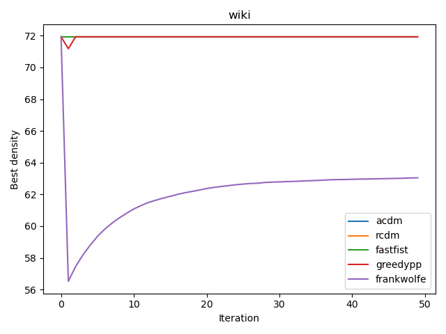
(a) wiki-topcats

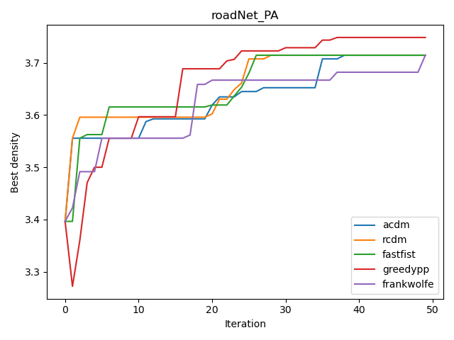
(b) roadNet-PA

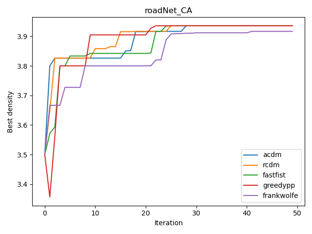
(c) roadNet-CA

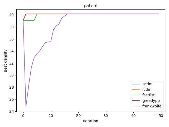
(d) cit-Patent

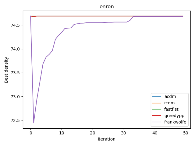
(e) com-Enron

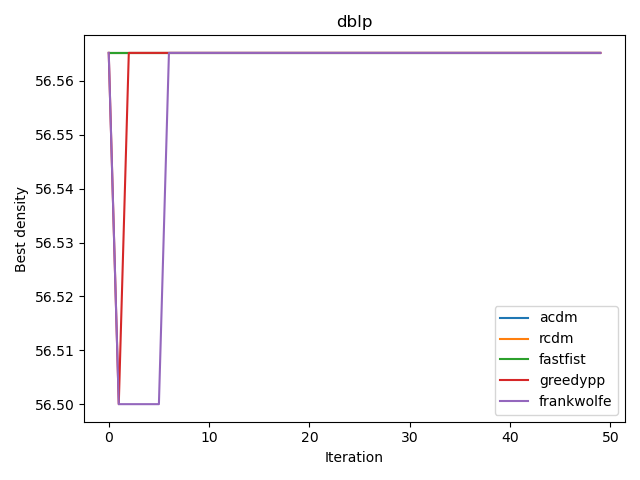
(f) dblp-author

Figure 2: Iteration/Best Density

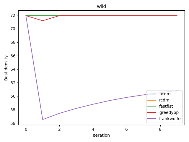
(a) wiki-topcats

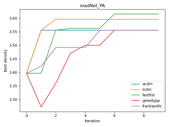
(b) roadNet-PA

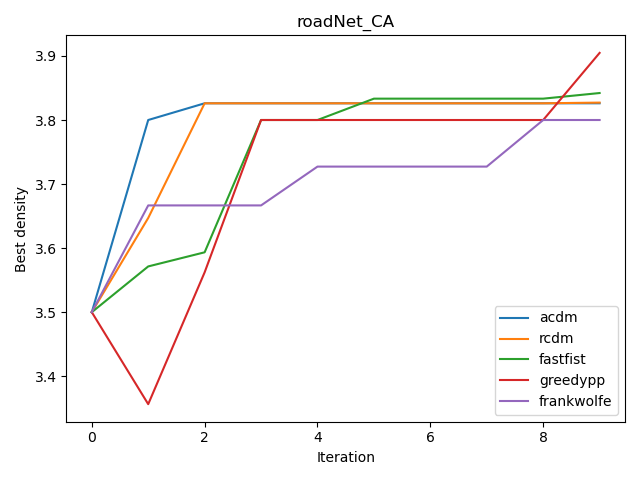
(c) roadNet-CA

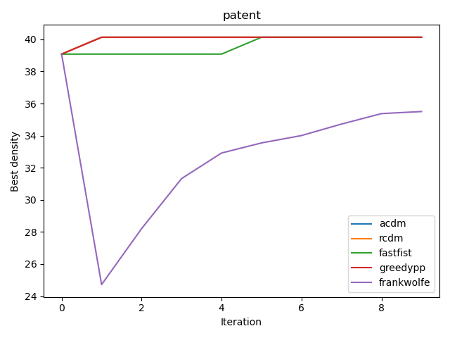
(d) cit-Patent

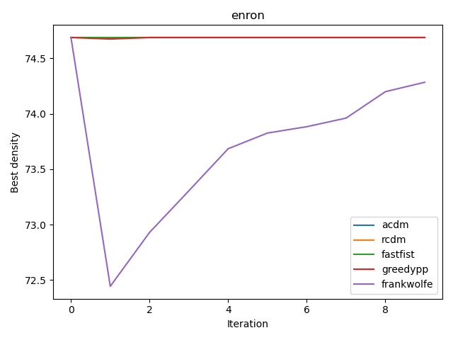
(e) com-Enron

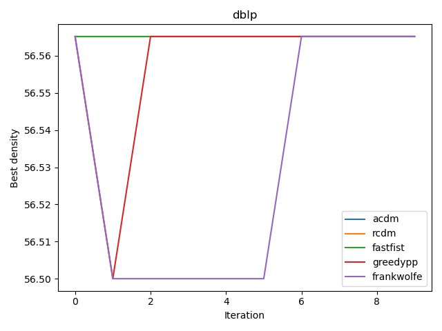
(f) dblp-author

Figure 3: Iteration/Best Density zoomed in the first 10 iterations

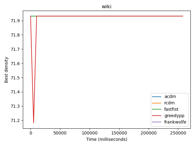
(a) wiki-topcats

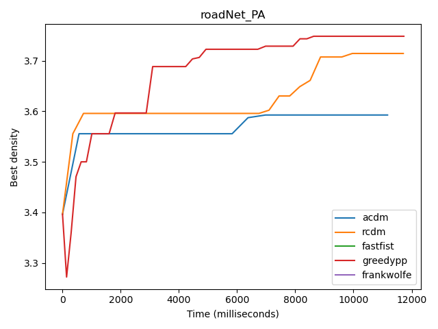
(b) roadNet-PA

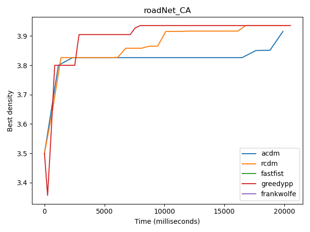
(c) roadNet-CA

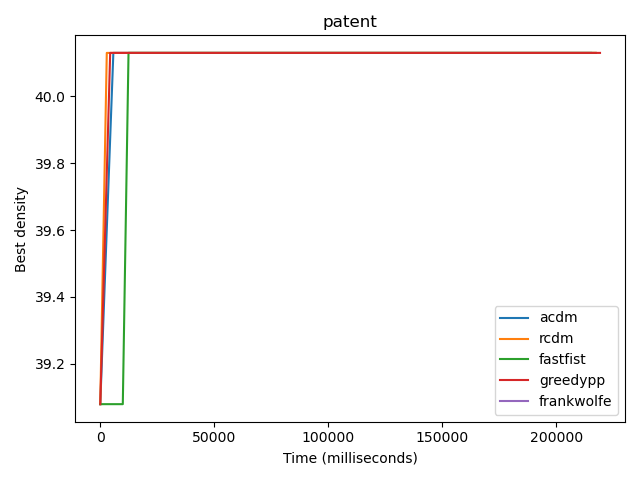
(d) cit-Patent

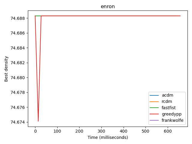
(e) com-Enron

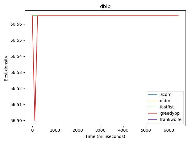
(f) dblp-author

Figure 4: Time/Best Density

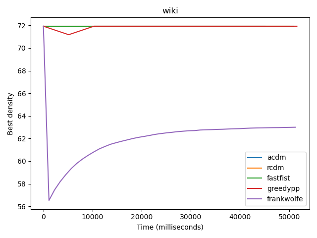
(a) wiki-topcats

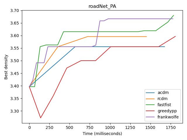
(b) roadNet-PA

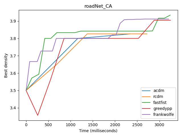
(c) roadNet-CA

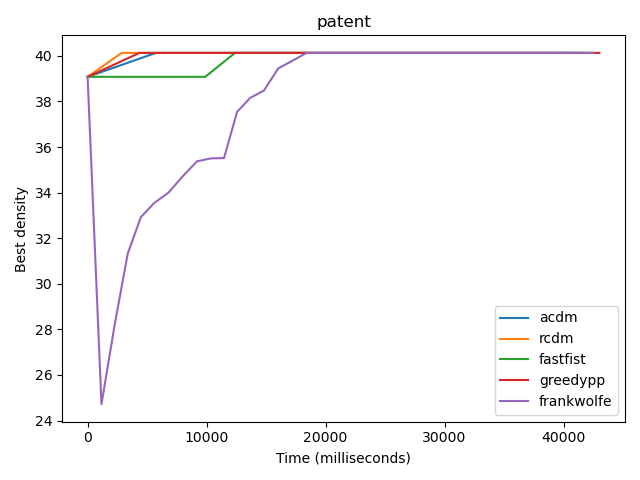
(d) cit-Patent

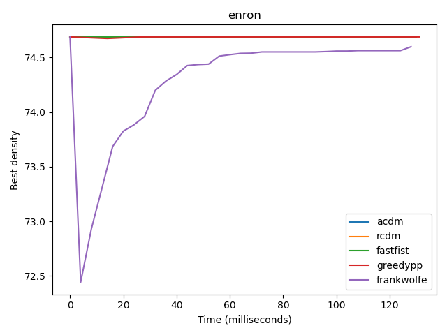
(e) com-Enron

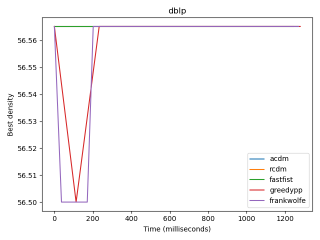
(f) dblp-author

Figure 5: Time/Best Density zoomed in the first iterations

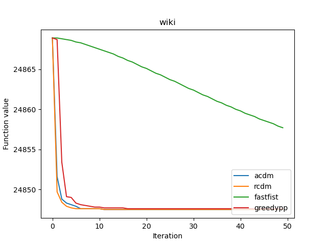
(a) wiki-topcats

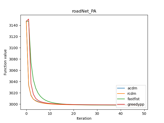
(b) roadNet-PA

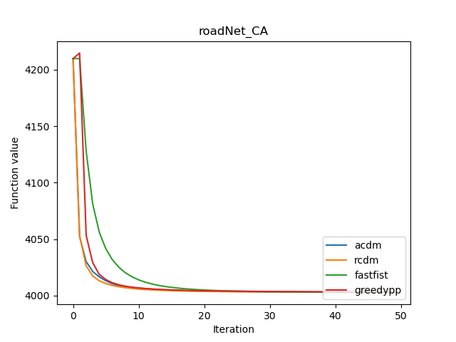
(c) roadNet-CA

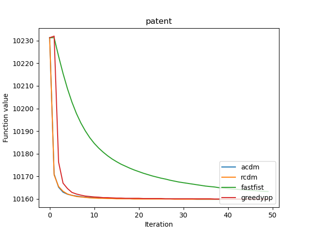
(d) cit-Patent

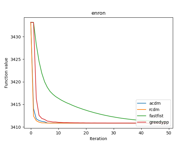
(e) com-Enron

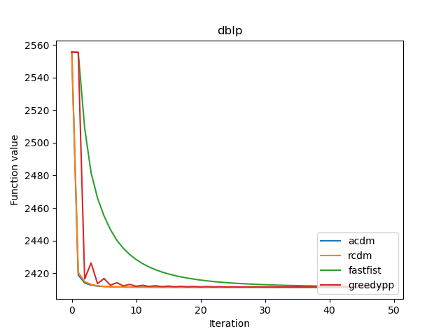
(f) dblp-author

Figure 6: Iteration/Load norm $\left(\sum_{u\in V}b_{u}^{2}\right)^{1/2}$. We exclude Frank-Wolfe from this plot as it performs significantly worse than the other algorithms

References

• Arora et al. (2012) Sanjeev Arora, Elad Hazan, and Satyen Kale. The multiplicative weights update method: a meta-algorithm and applications. Theory of computing, 8(1):121–164, 2012.
• Assadi et al. (2022) Sepehr Assadi, Arun Jambulapati, Yujia Jin, Aaron Sidford, and Kevin Tian. Semi-streaming bipartite matching in fewer passes and optimal space. In Proceedings of the 2022 Annual ACM-SIAM Symposium on Discrete Algorithms (SODA), pages 627–669. SIAM, 2022.
• Bahmani et al. (2012) Bahman Bahmani, Ravi Kumar, and Sergei Vassilvitskii. Densest subgraph in streaming and mapreduce. arXiv preprint arXiv:1201.6567, 2012.
• Bahmani et al. (2014) Bahman Bahmani, Ashish Goel, and Kamesh Munagala. Efficient primal-dual graph algorithms for mapreduce. In International Workshop on Algorithms and Models for the Web-Graph, pages 59–78. Springer, 2014.
• Beck (2015) Amir Beck. On the convergence of alternating minimization for convex programming with applications to iteratively reweighted least squares and decomposition schemes. SIAM Journal on Optimization, 25(1):185–209, 2015.
• Beck and Teboulle (2009) Amir Beck and Marc Teboulle. A fast iterative shrinkage-thresholding algorithm for linear inverse problems. SIAM journal on imaging sciences, 2(1):183–202, 2009.
• Boob et al. (2019) Digvijay Boob, Saurabh Sawlani, and Di Wang. Faster width-dependent algorithm for mixed packing and covering lps. Advances in Neural Information Processing Systems, 32, 2019.
• Boob et al. (2020) Digvijay Boob, Yu Gao, Richard Peng, Saurabh Sawlani, Charalampos Tsourakakis, Di Wang, and Junxing Wang. Flowless: Extracting densest subgraphs without flow computations. In Proceedings of The Web Conference 2020, pages 573–583, 2020.
• Charikar (2000) Moses Charikar. Greedy approximation algorithms for finding dense components in a graph. In International workshop on approximation algorithms for combinatorial optimization, pages 84–95. Springer, 2000.
• Chekuri et al. (2022) Chandra Chekuri, Kent Quanrud, and Manuel R Torres. Densest subgraph: Supermodularity, iterative peeling, and flow. In Proceedings of the 2022 Annual ACM-SIAM Symposium on Discrete Algorithms (SODA), pages 1531–1555. SIAM, 2022.
• Chen et al. (2022) Li Chen, Rasmus Kyng, Yang P Liu, Richard Peng, Maximilian Probst Gutenberg, and Sushant Sachdeva. Maximum flow and minimum-cost flow in almost-linear time. In 2022 IEEE 63rd Annual Symposium on Foundations of Computer Science (FOCS), pages 612–623. IEEE, 2022.
• Danisch et al. (2017) Maximilien Danisch, T-H Hubert Chan, and Mauro Sozio. Large scale density-friendly graph decomposition via convex programming. In Proceedings of the 26th International Conference on World Wide Web, pages 233–242, 2017.
• Dhulipala et al. (2022) Laxman Dhulipala, Quanquan C Liu, Sofya Raskhodnikova, Jessica Shi, Julian Shun, and Shangdi Yu. Differential privacy from locally adjustable graph algorithms: k-core decomposition, low out-degree ordering, and densest subgraphs. In 2022 IEEE 63rd Annual Symposium on Foundations of Computer Science (FOCS), pages 754–765. IEEE, 2022.
• Ene and Nguyen (2015) Alina Ene and Huy Nguyen. Random coordinate descent methods for minimizing decomposable submodular functions. In International Conference on Machine Learning, pages 787–795. PMLR, 2015.
• Ene et al. (2017) Alina Ene, Huy Nguyen, and László A Végh. Decomposable submodular function minimization: discrete and continuous. Advances in neural information processing systems, 30, 2017.
• Faragó and R. Mojaveri (2019) András Faragó and Zohre R. Mojaveri. In search of the densest subgraph. Algorithms, 12(8):157, 2019.
• Gallo et al. (1989) Giorgio Gallo, Michael D Grigoriadis, and Robert E Tarjan. A fast parametric maximum flow algorithm and applications. SIAM Journal on Computing, 18(1):30–55, 1989.
• Gionis and Tsourakakis (2015) Aristides Gionis and Charalampos E Tsourakakis. Dense subgraph discovery: Kdd 2015 tutorial. In Proceedings of the 21th ACM SIGKDD International Conference on Knowledge Discovery and Data Mining, pages 2313–2314, 2015.
• Goldberg (1984) Andrew V Goldberg. Finding a maximum density subgraph. 1984.
• Harb et al. (2022) Elfarouk Harb, Kent Quanrud, and Chandra Chekuri. Faster and scalable algorithms for densest subgraph and decomposition. Advances in Neural Information Processing Systems, 35:26966–26979, 2022.
• Harb et al. (2023) Elfarouk Harb, Kent Quanrud, and Chandra Chekuri. Convergence to lexicographically optimal base in a (contra) polymatroid and applications to densest subgraph and tree packing. arXiv preprint arXiv:2305.02987, 2023.
• Jambulapati and Tian (2023) Arun Jambulapati and Kevin Tian. Revisiting area convexity: Faster box-simplex games and spectrahedral generalizations. arXiv preprint arXiv:2303.15627, 2023.
• Jambulapati et al. (2019) Arun Jambulapati, Aaron Sidford, and Kevin Tian. A direct tilde $\{$O$\}$(1/epsilon) iteration parallel algorithm for optimal transport. Advances in Neural Information Processing Systems, 32, 2019.
• Kunegis (2013) Jérôme Kunegis. Konect: the koblenz network collection. In Proceedings of the 22nd international conference on world wide web, pages 1343–1350, 2013.
• Lanciano et al. (2023) Tommaso Lanciano, Atsushi Miyauchi, Adriano Fazzone, and Francesco Bonchi. A survey on the densest subgraph problem and its variants. arXiv preprint arXiv:2303.14467, 2023.
• Lee et al. (2010) Victor E Lee, Ning Ruan, Ruoming Jin, and Charu Aggarwal. A survey of algorithms for dense subgraph discovery. Managing and mining graph data, pages 303–336, 2010.
• Leskovec and Krevl (2014) Jure Leskovec and Andrej Krevl. Snap datasets: Stanford large network dataset collection, 2014.
• Nishihara et al. (2014) Robert Nishihara, Stefanie Jegelka, and Michael I Jordan. On the convergence rate of decomposable submodular function minimization. Advances in Neural Information Processing Systems, 27, 2014.
• Sherman (2017) Jonah Sherman. Area-convexity, l$\infty$ regularization, and undirected multicommodity flow. In Proceedings of the 49th Annual ACM SIGACT Symposium on Theory of Computing, pages 452–460, 2017.
• Su and Vu (2019) Hsin-Hao Su and Hoa T Vu. Distributed dense subgraph detection and low outdegree orientation. arXiv preprint arXiv:1907.12443, 2019.
• Tatti and Gionis (2015) Nikolaj Tatti and Aristides Gionis. Density-friendly graph decomposition. In Proceedings of the 24th International Conference on World Wide Web, pages 1089–1099, 2015.
• (32) Charalampos Tsourakakis and Tianyi Chen. Dense subgraph discovery: Theory and application (tutoral at sdm 2021).