BRACTIVE: A Brain Activation Approach to
Human Visual Brain Learning

Abstract

The human brain is a highly efficient processing unit, and understanding how it works can inspire new algorithms and architectures in machine learning. In this work, we introduce a novel framework named Brain Activation Network (BRACTIVE), a transformer-based approach to studying the human visual brain. The main objective of BRACTIVE is to align the visual features of subjects with corresponding brain representations via fMRI signals. It allows us to identify the brain’s Regions of Interest (ROI) of the subjects. Unlike previous brain research methods, which can only identify ROIs for one subject at a time and are limited by the number of subjects, BRACTIVE automatically extends this identification to multiple subjects and ROIs. Our experiments demonstrate that BRACTIVE effectively identifies person-specific regions of interest, such as face and body-selective areas, aligning with neuroscience findings and indicating potential applicability to various object categories. More importantly, we found that leveraging human visual brain activity to guide deep neural networks enhances performance across various benchmarks. It encourages the potential of BRACTIVE in both neuroscience and machine intelligence studies.

1 Introduction

Artificial intelligence (AI) algorithms [15, 36, 16, 63] have recently made significant capabilities one step forward to a human-like level, thanks to the development of deep learning. Inspired by human brain mechanisms, the feedforward and deep neural networks have greatly enhanced performance across various domains such as computer vision, natural language processing, speech recognition, etc [44, 48, 45, 42, 76, 51, 43, 46, 49, 41, 47, 68]. Recent studies show that these methods are more likely to mirror the mechanism of the human brain. For instance, a relationship has been found between brain representations in the visual pathway and the hierarchical layers within Deep Neural Networks (DNNs) [26, 8, 23, 80, 9]. They have lighted a research direction involving both cognitive neuroscientists and AI researchers to uncover the mechanisms and complexities of the human brain and then potentially adapting these findings to AI models [70, 57, 53, 71].

In one direction, brain-inspired representations offer a promising avenue for enhancing DNNs training. For example, incorporating brain data, such as Electroencephalogram (EEG) signals, has been shown to improve performance in classification and salient detection tasks [56]. Another study showed that representations simulating the primate primary visual cortex in DNN models significantly enhance robustness to adversarial attacks and image corruptions [13]. This approach leverages the inherent strengths of neural processing to guide and refine artificial models. Conversely, AI models possess unique capabilities that can significantly advance our understanding of neuroscience [5, 60, 4]. These models can simulate complex neural interactions and offer insights that are challenging to obtain through traditional experimental methods. Specifically, our research highlights the advantages of integrating deep learning techniques with neuroscience to elucidate the topological representations of objects within the brain. By mapping these representations, we can gain a deeper understanding of how the brain organizes and processes visual information.

Contribution of This Work. In summary, the contributions in this paper are four-folds. First, we present a novel transformer-based Brain Activation Network (BRACTIVE) for human visual brain understanding. Apart from the prior work, our approach can identify the brain’s Regions of Interest (ROI) of multiple subjects automatically as in Fig. 1. Second, we propose a novel module named Subject of Interest Proposal (SOIP) to predict the interested subjects that participants are focusing on during the visual tasks. Third, since the labels for the proposed tasks are not available, we introduce the Subject of Interest Retrieval (SOIR) module to establish features of these subjects in visual and fMRI modalities. Finally, the Weighted SOI Loss function is presented to align the features of subjects across modalities. The experiments show ROIs for humans identified by BRACTIVE are closely aligned with the findings (floc-faces, floc-bodies) from neuroscience. It promises to bring valuable references for neuroscientists in studying visual brain functions. The will be released.

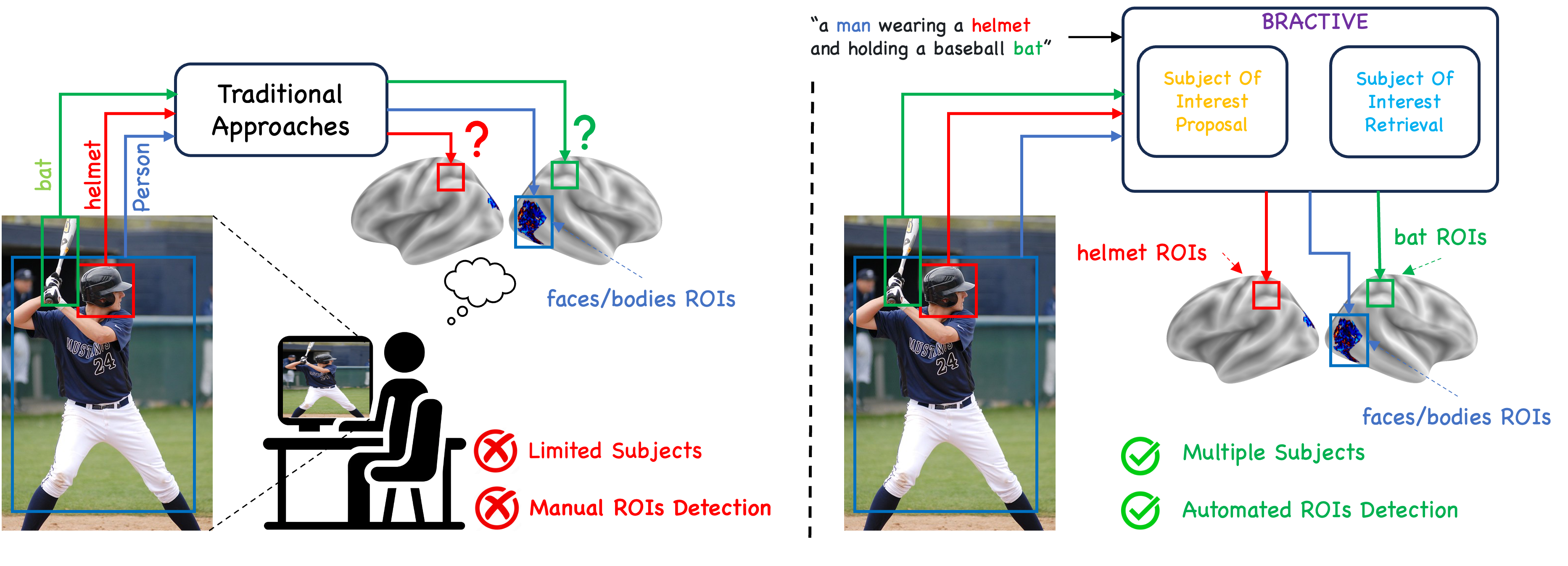
Figure 1: The proposed method can automatically determine the subject of interest and corresponding ROIs inside the brain that the participant is focusing on.

2 Related Work

Decoding human brain representation has been one of the most popular research topics for a decade. In particular, cognitive neuroscience has made substantial advances in understanding neural representations originating in the primary Visual Cortex (V1) [69]. Indeed, the primary visual context is responded to process information related to oriented edges and colors. The V1 forwards the information to other neural regions, focusing more on complex shapes and features. These regions are largely overlapped with receptive fields such as V4 [58], before converging on object and category representations in the inferior temporal (IT) cortex [10]. Neuroimaging techniques, including Functional Magnetic Resonance Imaging(fMRI), Magnetoencephalography(MEG), and electroencephalogram(EEG), have been crucial in these studies. However, to replicate human-level neural representations that fully capture our visual processes, it is crucial to precisely monitor the activity of every neuron in the brain simultaneously. Consequently, recent efforts in brain representation decoding have focused on exploring the correlation between neural activity data and computational models. In this research direction, several studies [25, 73, 27, 11, 24] were presented to decode brain information. Recently, with the help of deep learning, the authors in [7, 66, 72, 55, 33, 54] presented the methods to reconstruct what humans see from fMRI signal using diffusion models. The authors in [30, 7] also explored patterns of fMRI signals. However, they often fall short of demonstrating or explaining the nature of these patterns.

In addition, there are recent studies on the intersection between AI and cognitive neuroscience [74, 75, 28, 61, 33, 39, 18, 64, 35, 59, 29, 12, 65, 17, 32, 74, 62, 49]. Deep learning methods [1, 79, 81, 31, 50] have been applied to predict the neural responses. Some other studies inspired by biological mechanisms such as memory [21], coding theory, and attention [22, 78] are increasingly adopted in the AI field. Some recent methods have used neural activity data to guide the training of models [56, 19, 70, 52, 40]. They utilized EEG and fMRI signals to constrain the neural network to behave like the neural response in the visual cortex.

Discussion: Neuroscience and computer science mutually benefit each other. Insights from the human cognitive system can lead to innovative AI algorithms, while advanced deep neural networks can enhance our exploration of the human brain. By delving deeper into the intricacies of how the brain processes information, learns, and makes decisions, researchers are paving the way for a new era of AI. This understanding can be translated into more efficient AI solutions that require less training data and can learn and adapt in ways that mirror human learning. According to neuroscience findings, V1 is responsible for edge, and orientation processing, while V4 can handle larger receptive fields. The object-specific ROIs such as floc-faces and floc-bodies are responsible for recognizing human subjects. This prompts the question: Which Regions of Interest (ROIs) are related to processing information of other subjects, such as animals, bicycles, cars, etc?. Therefore, this paper focuses on understanding how the human visual brain processes visual stimuli. Apart from the prior studies, our approach is not limited by predefined visual ROI from the neuroscience field. Instead, the proposed method can automatically explore more ROI for a specific subject.

3 The Proposed Brain Activation Network Approach

In this section, we detail the proposed method. In particular, we first briefly introduce vision encoder, fMRI encoder, and text encoder in Subsections 3.1, 3.2, 3.3, respectively. Then, the details of the Subject of Interest Proposal, Subject of Interest Retrieval modules, and overall objective loss functions are presented in Subsections 3.4, 3.5, 3.6, correspondingly.

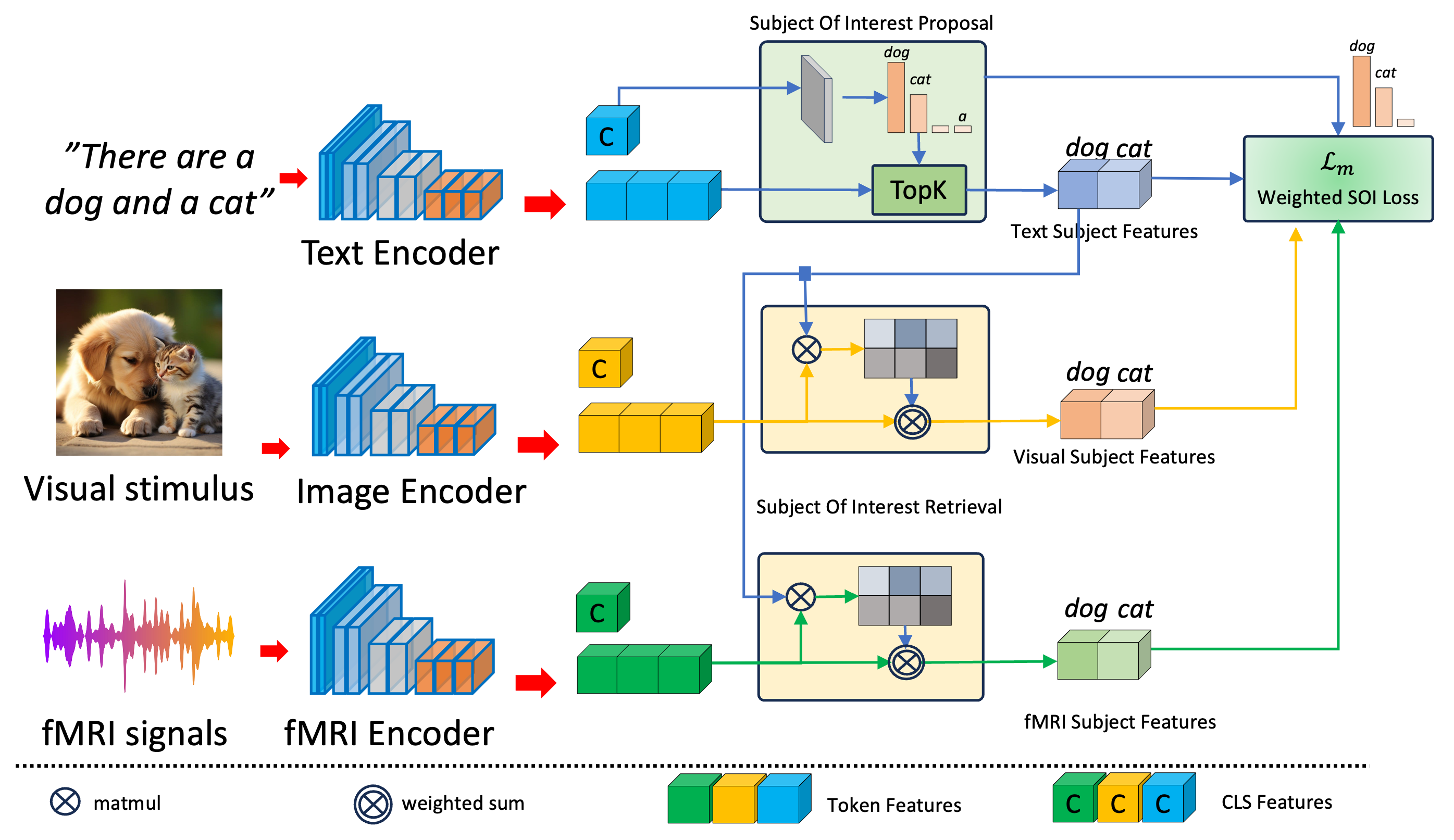
Figure 2: The illustration of BRACTIVE and training objectives. The Subject of Interest Proposal proposes the interested subjects that the participants are focusing on. The Subject of Interest Retrieval is used to construct the corresponding features of the proposed subjects on visual and fMRI modalities. The Weighted SOI Loss is used to align the features of these subjects.

3.1 Vision Encoder

Given a visual stimulus $x\in\mathbb{R}^{h\times w\times c}$, we split $x$ into multiple non-overlap patches $\mathcal{P}=\{p_{i}\}_{i=0}^{N_{p}-1}$ where $N_{p}=|\mathcal{P}|=(h\times w)/{p^{2}}$ is the number of patches, and $p$ is the patch size. Let $\texttt{Enc}_{v}$ be a visual encoder, i.e., ViT, which receives $\mathcal{P}$ as the input. The vectors of latent and patches are represented as in the Eq. (1).

$$\mathbf{P}_{\texttt{CLS}},\left[\mathbf{P}_{0},\dots\mathbf{P}_{i},\dots\mathbf{P}_{N_{p}-1}\right]=\texttt{Enc}_{v}(\mathcal{P})\quad\mathbf{P}_{\texttt{CLS}}\in\mathbb{R}^{1\times d},\mathbf{P}_{i}\in\mathbb{R}^{1\times d}$$ (1)

where $\mathbf{P}_{i}$ is the feature vector of the $i^{th}$ patch and $\mathbf{P}_{\texttt{CLS}}$ is the feature vector representing context in the visual stimulus $x$. Since $\texttt{Enc}_{v}$ is a transformer-based architecture, we can write $\mathbf{P}_{\texttt{CLS}}=\sum_{i=0}^{N_{p}-1}\alpha_{i}\mathbf{P}_{i}$ where $\sum\alpha_{i}=1$ and $0\leq\alpha_{i}\leq 1$. Similarly, consider a subject $s_{k}$ appears in $x$, the visual feature of $s_{k}$ can be represented in the Eqn (1)

$$\mathbf{P}_{s_{k}}=\sum_{i=0}^{N_{p}-1}\alpha_{ik}\mathbf{P}_{i}$$ (2)

where $\alpha_{ik}$ acts as a coefficient, expressing how much the texture of $s_{k}$ is included in $p_{i}$.

Remark 1.

By finding the coefficient $\alpha_{ik}$, we can determine the regions or patches in the image that correspond to $\mathbf{P}_{s_{k}}$.

3.2 fMRI Encoder

In dealing with the high-dimensional fMRI 1D signal $f\in\mathbb{R}^{N_{F}}$, where $N_{F}$ might reach 100K, a direct strategy involves employing linear or fully connected layers [66] to model the signal and derive its latent embedding. However, this approach encounters two main limitations. First, fully connected layers struggle with high-dimensional features, making it difficult to extract meaningful information while burdening the model’s memory usage. Second, the current representation form of the fMRI, as a signal, makes it difficult to explore the local patterns of nearby voxels (Please refer to the Appendix/Supplementary sections for the details). To address these challenges, we project these signals into a flattened 2D space by leveraging the transformation function of fsaverage surface. Then we have $f_{2d}=\texttt{T}_{2d}(f)\in\mathbb{R}^{h_{2d}\times w_{2d}}$ where $f_{2d}$ is the flattened 2D form of the fMRI signal $f$, $h_{2d}$ and $w_{2d}$ are the height and width, correspondingly. Consequently, we apply a transformer-based encoder, denoted $\texttt{Enc}_{f}$, to extract its feature. The output features of the fMRI signals are represented as in Eq. (3).

$$\mathbf{F}_{\texttt{CLS}},\left[\mathbf{F}_{0},\dots\mathbf{F}_{i},\dots\mathbf{F}_{N_{r}-1}\right]=\texttt{Enc}_{f}(f_{2d})\quad\mathbf{F}_{\texttt{CLS}}\in\mathbb{R}^{1\times d},\mathbf{F}_{i}\in\mathbb{R}^{1\times d}$$ (3)

Similar to the visual encoder, the fMRI features of the subject $s_{k}$ is defined as in Eqn (4)

$$\mathbf{F}_{s_{k}}=\sum_{i=0}^{N_{r}-1}\beta_{ik}\mathbf{F}_{i}$$ (4)

Remark 2.

By finding the coefficient $\beta_{ik}$, we can determine the sub-signals/voxels in the fMRI that correspond to $\mathbf{F}_{s_{k}}$.

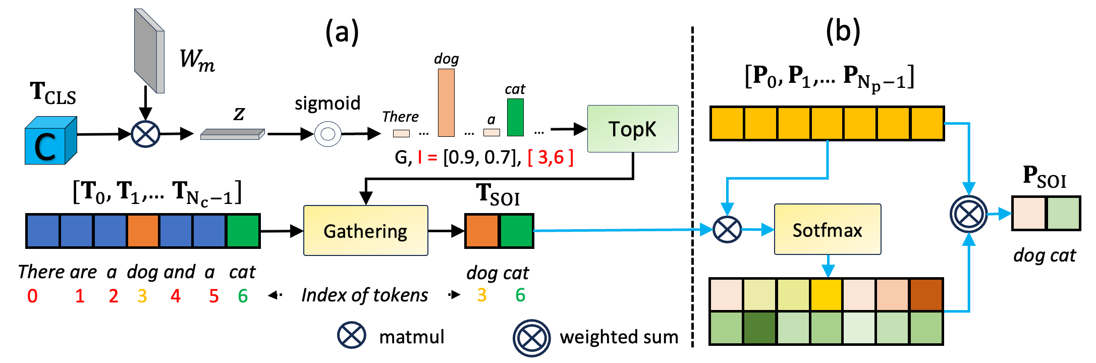
Figure 3: Detailed illustration of Subject of Interest Proposal (SOIP) (a) Subject of Interest Retrieval (SOIR) (b) module. It is similar to applying the SOIR module for the fMRI modality by replacing vision tokens $\textbf{P}_{i}$ by $\textbf{F}_{i}$, respectively

3.3 Text Encoder

Since $\mathbf{P}_{s_{k}}$ and $\mathbf{F}_{s_{k}}$ represent the visual and fMRI modalities of the $s_{k}$ subject, respectively, we need semantic labels in visual to construct these features. However, we need prior access to this information, posing a significant obstacle. To address this challenge, we propose utilizing the text modality to represent the $s_{k}$ for the following reasons. First, unlike the visual and fMRI modalities that require multiple patches or pixels and sub-signals/voxels to represent the subject, a single word is sufficient to describe the subject (e.g., cat, dog, etc.) in the text modality. Secondly, the features of the text are more discriminative than images, thanks to BERT-based architecture [bert]. Thus, text poses a strong representation of a subject.

Let $t$ be the text description describing the visual stimulus context $x$. We assume that $t$ contains the word represent for the subjects inside $x$. Following prior work [63, 16], we use transformer-based architecture to extract the features of $t$ as following:

$$\mathbf{T}_{\texttt{CLS}},\left[\mathbf{T}_{0},\dots\mathbf{T}_{i},\dots\mathbf{T}_{N_{c}-1}\right]=\texttt{Enc}_{t}(\mathbf{t})\quad\mathbf{T}_{\texttt{CLS}}\in\mathbb{R}^{1\times d},\mathbf{T}_{i}\in\mathbb{R}^{1\times d}$$ (5)

Similar to visual and fMRI modalities, we have $\textbf{T}_{s_{k}}$ to represent context feature and text features of $s_{k}$, respectively. However, $\textbf{T}_{s_{k}}$ is not a combination of any tokens in the $t$, instead, $\textbf{T}_{s_{k}}\in\left[\mathbf{T}_{0},\dots\mathbf{T}_{i},\dots\mathbf{T}_{N_{c}-1}\right]$ is one of tokens in $t$. In the next section, we present the new Subject of Interest Proposal module to determine which token represents the $s_{k}$.

3.4 Subject of Interest Proposal

1:  Input: The visual stimulus $x$, fMRI signal $f$, text description $t$. Let $k$ be the number of the subject of interest proposal. 2:  Output: The objective loss. $\triangleright$ Extract visual features 3:  $\mathcal{P}\leftarrow\texttt{Patchify}(x)$ 4:  $\mathbf{P}_{\texttt{CLS}},\left[\mathbf{P}_{0},\dots\mathbf{P}_{i},\dots\mathbf{P}_{N_{p}-1}\right]\leftarrow\texttt{Enc}_{v}(\mathcal{P})$ $\triangleright$ Extract fMRI features 5:  $f_{2d}\leftarrow\texttt{T}_{2d}(f)$ 6:  $\mathbf{F}_{\texttt{CLS}},\left[\mathbf{F}_{0},\dots\mathbf{F}_{i},\dots\mathbf{F}_{N_{r}-1}\right]\leftarrow\texttt{Enc}_{f}(f_{2d})$ $\triangleright$ Extract text features 7:  $\mathbf{T}_{\texttt{CLS}},\left[\mathbf{T}_{0},\dots\mathbf{T}_{i},\dots\mathbf{T}_{N_{c}-1}\right]\leftarrow\texttt{Enc}_{t}(t)$ $\triangleright$ Subject of interest proposal 8:  $\mathbf{T}_{\texttt{SOI}},G\leftarrow\texttt{SOIP}(\mathbf{T}_{\texttt{CLS}},k)$ $\triangleright$ Subject of interest retrieval 9:  $\mathbf{P}_{\texttt{SOI}}\leftarrow\texttt{SOIR}(\mathbf{T}_{\texttt{SOI}},\mathbf{P}_{v})$ 10:  $\mathbf{T}_{\texttt{SOI}}\leftarrow\texttt{SOIR}(\mathbf{F}_{\texttt{SOI}},\mathbf{F}_{f})$ $\triangleright$ Global contextual loss 11:  $\mathcal{L}_{g}\leftarrow\texttt{TripContras}(\mathbf{T}_{\texttt{CLS}},\mathbf{P}_{\texttt{CLS}},\mathbf{F}_{\texttt{CLS}})$ $\triangleright$ Subject of interest loss 12:  $\mathcal{L}_{m}\leftarrow 0$ 13:  for $k^{\prime}=1,\cdots,k$ do 14:     $\mathbf{T}_{s_{k}},\mathbf{P}_{s_{k}},\mathbf{F}_{s_{k}}\leftarrow\mathbf{T}_{\texttt{SOI}}\left[k^{\prime}\right],\mathbf{P}_{\texttt{SOI}}\left[k^{\prime}\right],\mathbf{F}_{\texttt{SOI}}\left[k^{\prime}\right]$ 15:     $\mathcal{L}_{m}\leftarrow\mathcal{L}_{m}+G\left[k^{\prime}\right]*\texttt{WeightedSOILOss}(\mathbf{T}_{s_{k}},\mathbf{P}_{s_{k}},\mathbf{F}_{s_{k}})$ 16:  end for 17:  $\mathcal{L}=\lambda_{g}\mathcal{L}_{g}+\lambda_{m}\mathcal{L}_{m}$ 18:  return $\mathcal{L}$

Algorithm 1 Pseudo code of BRACTIVE.

Let $\mathcal{M}_{s}$ be a set of subjects within a visual stimulus that the participant is focusing. It is crucial to recognize that $\mathcal{M}_{s}$ varies for each individual. For instance, in a stimulus containing both dogs and cats, a person fond of dogs will focus solely on the regions containing dogs, while cat lovers will concentrate on the cats’ regions. Consequently, identifying $\mathcal{M}_{s}$ poses a challenge since we need to possess this predefined set of subjects of interest in advance. To address this challenge, we introduce the SOIP module to identify $\mathcal{M}_{s}$.

Since $\mathbf{T}_{\texttt{CLS}}$ encapsulates the entire context of the visual input $x$, we employ this feature as the input of SOIP for predicting which token $t_{i}\in t$ signifies the interested subject. To achieve this, we establish a trainable matrix $W_{m}\in\mathbb{R}^{N_{c}\times d}$ to transform $\textbf{T}_{\texttt{CLS}}$ into a logit vector $z\in\mathbb{R}^{1\times N_{c}}$. Each element $z_{i}\in z$ corresponds to the probability of token $t_{i}$ representing a subject of focus. Considering the possibility of multiple interested subjects, we utilize the sigmoid function on $z$ instead of softmax. Here, $k$ denotes the potential number of interested subjects within the visual input $x$, and we utilize the topK function to select the $k$ tokens with the highest likelihood of representing interested subjects. Mathematically, the SOIP is described as in Eq. (6).

$$\begin{split}z&=\texttt{sigmoid}(\textbf{T}_{\texttt{CLS}}\otimes W_{m}^{\top})\quad\text{, }W_{m}\in\mathbb{R}^{N_{c}\times d},z\in\mathbb{R}^{1\times N_{c}}\\ G,I&=\texttt{TopK}(z,k)\quad\text{, }G\in\mathbb{R}^{k},I\in\mathbb{N}^{+k}\\ \mathbf{T}_{\texttt{SOI}}&=\left[\textbf{T}_{i}\right]_{i\in I}\end{split}$$ (6)

Where $I$ is a vector stating the location of the token in the $t$ and $G$ is a vector representing the corresponding probability. $\mathbf{T}_{\texttt{SOI}}$ is the a feature set of $\mathcal{M}_{s}$ where each element is the token feature $\textbf{T}_{i}$ as defined in the Eq. (5) where $i\in I$.

Remark 3.

The $\mathbf{P}_{s_{k}}$, $\mathbf{F}_{s_{k}}$ and $\mathbf{T}_{s_{k}}$ are features of the same subject. They are equivalent in subject representation if aligned in the same domain space.

3.5 Subject of Interest Retrieval

As outlined in the previous section, it is infeasible to directly form $\textbf{P}_{s_{k}}$ and $\textbf{F}_{s_{k}}$. The Remark 1 and Remark 2 imply that if we can find the coefficient $\alpha_{ik}$, we can measure them directly. Fortunately, according to the Remark 3, $\mathbf{P}_{s_{k}}$, $\mathbf{F}_{s_{k}}$ and $\mathbf{T}_{s_{k}}$ are equivalent, but in the form of different modalities. Therefore, we measure the coefficient $\alpha_{ik}$ by measuring the similarity of $\mathbf{T}_{s_{k}}$ and each token. Motivated by this idea, we introduce the SOIR module to construct the features of interested subjects in visual and fMRI modalities. We detail how this module operates for visual $\textbf{P}_{s_{k}}$ and note that the approach is similarly applicable for $\textbf{F}_{s_{k}}$.

Given a sequence of visual tokens $\mathbf{P}_{v}=\left[\mathbf{P}_{0},\dots,\mathbf{P}_{i},\dots,\mathbf{P}_{N_{p}-1}\right]$. Firstly, we measure coefficient $\alpha_{ik}=\texttt{sim}(\mathbf{P}_{i},\textbf{T}_{s_{k}})$. After that, we use the softmax function over these coefficients to normalize the feature aggregation. Consequently, we form $\textbf{P}_{s_{k}}$ as the weighted sum of patches’ features as mentioned in the Section 3.2.

3.6 Objective Loss Functions

Global Contextual Loss. This loss function keeps the global context sharing between visual, text, and fMRI similar. In particular, let Contras be a contrastive loss function. The global context loss $\mathcal{L}_{g}$ is defined as in Eq. (7).

$$\begin{split}\mathcal{L}_{g}&=\texttt{Contras}(\textbf{T}_{\texttt{CLS}},\textbf{P}_{\texttt{CLS}})+\texttt{Contras}(\textbf{T}_{\texttt{CLS}},\textbf{F}_{\texttt{CLS}})+\texttt{Contras}(\textbf{F}_{\texttt{CLS}},\textbf{P}_{\texttt{CLS}})\\ \texttt{Contras}(x,y)&=-\frac{1}{N}\sum_{i}^{N}\log\frac{\exp({x}_{i}\otimes{y}_{i}/\sigma)}{\sum_{j}^{N}\exp({x}_{i}\otimes{y}_{j}/\sigma)}-\frac{1}{N}\sum_{i}^{N}\log\frac{\exp({y}_{i}\otimes{x}_{i}/\sigma)}{\sum_{j}^{N}\exp({y}_{i}\otimes{x}_{j}/\sigma)}\end{split}$$ (7)

Weighted SOI Loss. With the SOIP and SOIR modules, we get the features of the interested subjects in text, visual, and fMRI domains, respectively. It is crucial to learn similarities among them from the same subject and to distinguish them from those of distinct subjects. Similar to the global contextual loss mentioned earlier, we employ a contrastive loss function for each proposed subject. However, unlike the equation mentioned earlier, we incorporate a loss weight for each proposal. It is because, with a fixed number $k$ of proposed subjects, there may be instances where the number of minding subjects is less than $k$. Relying solely on the confidence score as a weight for the loss should aid SOIP in better learning and in reducing false positives in that module. The Weighted SOI Loss $\mathcal{L}_{m}$ is formulated as in Eq. (8).

$$\begin{split}\mathcal{L}_{m}=\sum_{i=0}^{k-1}G\left[i\right]\left(\texttt{Contras}(\mathbf{T}_{s_{i}},\mathbf{P}_{s_{i}})+\texttt{Contras}(\mathbf{T}_{s_{i}},\mathbf{F}_{s_{i}})+\texttt{Contras}(\mathbf{F}_{s_{i}},\mathbf{P}_{s_{i}})\right)\end{split}$$ (8)

In summary, the BRACTIVE is trained by the following loss function: $\mathcal{L}=\lambda_{g}\mathcal{L}_{g}+\lambda_{m}\mathcal{L}_{m}$, where $\lambda_{g}$ and $\lambda_{m}$ are the weights for two corresponding loss functions. Overall, the proposed method is described in the Algorithm 1.

4 Brain Region of Interest Localization

1:  Input: The features of the interested subject $\mathbf{F}_{s_{k}}\in\mathbb{R}^{1\times d}$, patches’ features of flattened fMRI 2D $\mathbf{F}_{f}\in\mathbb{R}^{N_{r}\times d}$, scale factor $s$, threshold $\gamma$ 2:  Output: The optimization loss function. 3:  $\mathbf{F}_{s_{k}}\leftarrow\texttt{l2norm}(\mathbf{F}_{s_{k}})$ 4:  $\mathbf{F}_{f}\leftarrow\texttt{l2norm}(\mathbf{F}_{f})$ 5:  $B\leftarrow\mathbf{F}_{s_{k}}\otimes\mathbf{F}_{f}^{\top}\in\mathbb{R}^{1\times N_{r}}$ 6:  $B\leftarrow\texttt{upsampling}(B,s)\in\mathbb{R}^{h_{2d}\times w_{2d}}$ 7:  $B\leftarrow\texttt{T}_{2d}^{\top}(B)\in\mathbb{R}^{N_{f}}$ 8:  $B\leftarrow B>\gamma$ 9:  return $B$

Algorithm 2 Pseudo code for ROIs detection.

As noted in Remark 2, the sub-signals or voxels in fMRI corresponding to a subject can be identified by evaluating the coefficient $\beta_{ik}$. This coefficient is defined as $\beta_{ik}=\texttt{sim}(\mathbf{F}_{s_{k}},\mathbf{F}i)$, representing the cosine similarity between $\mathbf{F}_{s_{k}}$ and $\mathbf{F}_{i}$. Additionally, a threshold $\gamma$ is predefined, designating that a sub-signal $f_{i}\in f$ is associated with the subject $s_{k}$ if $\beta_{ik}>\gamma$. The procedure for detecting the subject-specific fMRI signal is detailed in Algorithm 2. This algorithm highlights two principal observations. (1) Thanks to the Weighted SOI Loss, we can employ both kinds of features from the interested subjects, such as $\mathbf{T}_{s_{k}},\mathbf{P}_{s_{k}}$, as inputs of the algorithm. This flexibility allows for multiple approaches to be used in studying brain activities. Either text or vision modalities can be used to detect the ROIs of the subjects. (2) The Algorithm 2 can be adapted for visual analysis by substituting $\textbf{F}_{f}$ with $\mathbf{P}_{v}$. This modification allows us to identify which parts of an image strongly correlate with predetermined regions of interest (ROIs) in the brain.

5 Implementation Details

Visual Encoder and fMRI Encoder. We employ the ViT-B-16 for both visual and fMRI encoder. The input image size is $224\times 224$. The feature dimension of these encoders is set to 1024.
Text Encoder. We take the pretrained transformer architecture from [63] to extract features of the text. The maximum length of the context is set to 77 [63] and the dimension of text features is also set to 1024. The text encoder is frozen while training. It will help to align visual and fMRI features to the text features easily.
SOIP. For the SOIP module, we select $k=4$ while proposing the potential subject of interest.
Datasets. To train BRACTIVE, we use the Natural Scenes Dataset (NSD) [2], a comprehensive compilation of responses from eight participants obtained through high-quality 7T fMRI scans. Each subject was exposed to approximately 73,000 natural scenes, forming the basis for constructing visual brain encoding models. Since the visual stimulus in this database is a subset of COCO [34], for each sample, there exists captions (text modality), visual stimulus, and corresponding fMRI response, respectively. For each subject, we split the data into 5 folds for training and validation.
Training Strategy. BRACTIVE is implemented easily in Pytorch framework and trained by 16 $\times$ A100 GPUs (40G each). The learning rate is set to $2.5e^{-5}$ initially and then reduced to zero gradually under ConsineLinear [37] policy. The batch size is set to $4$/GPU. The model is optimized by AdamW [38] for $30$ epochs. The training is completed within two hours.

6 Experimental Results

6.1 Localized ROIs w.r.t Human

Table 1: The Dice Score of ROIs localization w.r.t human subjects. The AvgAtt is the average of the attention maps of human subjects across participants.

Method	P1	P2	P3	P4	P5	P6	P7	P8	AvgAtt
GradCAM [67]	57.36($\pm$ 0.3)	56.73($\pm$ 0.1)	58.32($\pm$ 0.2)	55.41($\pm$ 0.2)	60.78($\pm$ 0.1)	61.24($\pm$ 0.1)	59.29($\pm$ 0.3)	56.52($\pm$ 0.2)	54.84($\pm$ 0.2)
Ours	68.98($\pm$ 0.2)	69.32($\pm$ 0.2)	69.31($\pm$ 0.3)	69.84($\pm$ 0.1)	69.31($\pm$ 0.3)	69.70($\pm$ 0.1)	69.87($\pm$ 0.1)	69.37($\pm$ 0.3)	72.57($\pm$ 0.2)

Since the ROIs for specific subjects are limited, in the scope of this paper, we evaluate the accuracy of BRACTIVE with respect to human subjects only. In particular, we get the ROIs of floc-faces and floc-bodies areas inside the brain as the ground truth and evaluate how well our algorithm 2 could localize the ROIs of the human subjects. We utilize dice scores as the evaluation metric. The results are demonstrated in the Table 1. The details and visualization of the prediction and ground truth can be found in the supplementary section.

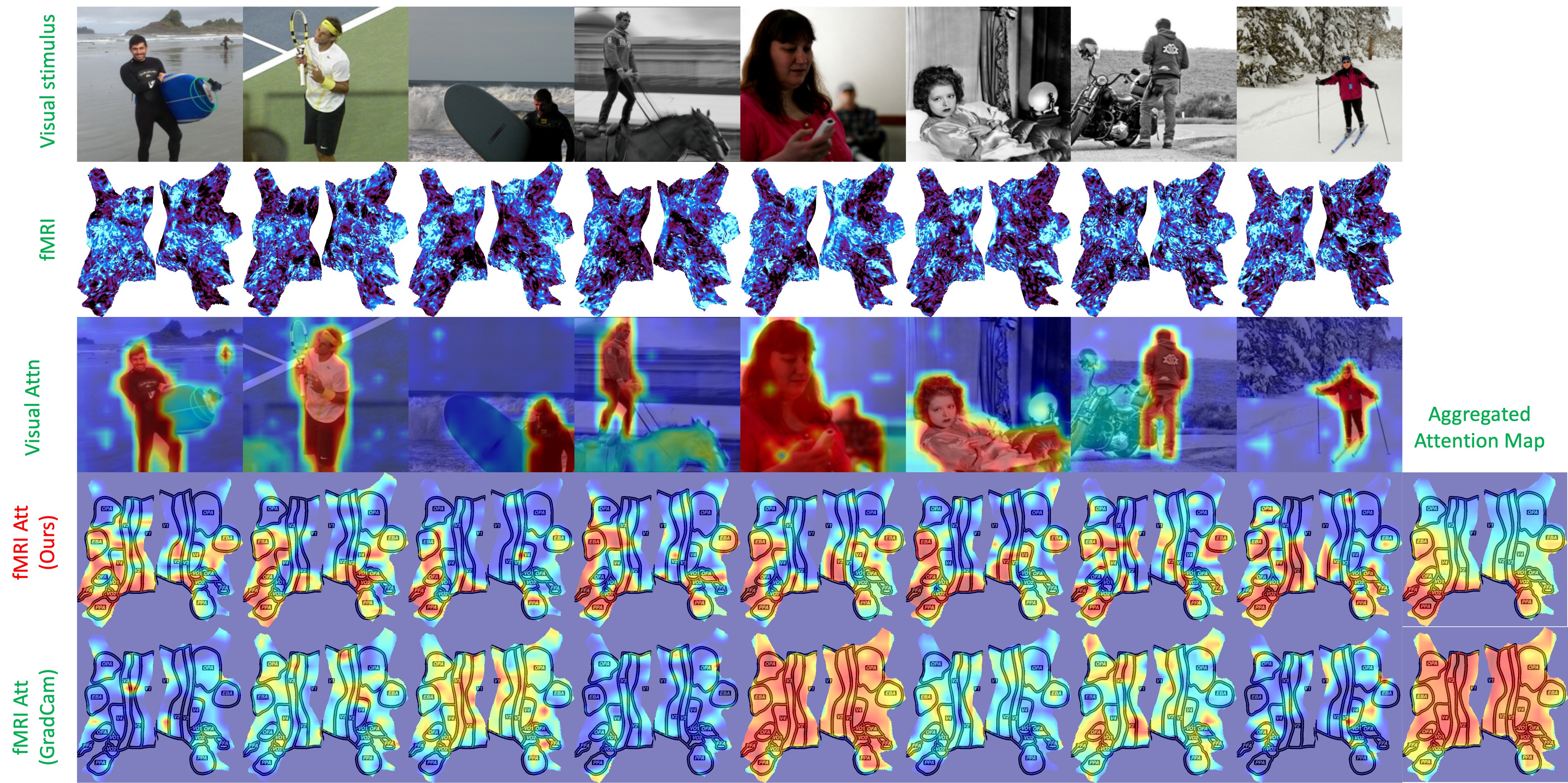
Figure 4: Region Of Interest of the human subject perceived by participant P1. The last column includes the mean of attention maps across all samples of all participants in the NSD. In the attention map, the brighter the colors, the higher correlation to the subject.

To establish a baseline for ROI localization, we employ ViT-B-16 as an fMRI encoder. We develop a classification model that processes fMRI signals and predicts the subject categories depicted in the visual stimuli. Since the visual stimulus from NSD belongs to the COCO database, our model targets classification into 80 fixed categories. Upon completing the training, we utilize GradCAM [67] to identify which regions correspond to specific subjects, such as humans or persons. We set a threshold in GradCAM to define the semantics of the ROIs. This baseline archives the dice score from 55.41% to 61.24% for eight participants.

In the second experiment, we use steps outlined in Algorithm 2 to localize the ROIs. Overall, we observe a notable enhancement ranging from 68% to 69% consistently across eight participants in comparison to the GradCam [67]. In the third experiment, we take the average of the attention maps across all participants. Surprisingly, the performance drops to 54.84 % for the GradCam [67] baseline while we observe a notable improvement of 72.57% from our method.

6.2 Brain Response Prediction

This downstream task aims to predict the neural responses of the human brain to natural scenes, as observed during participant viewing sessions [20, 1]. We employ the pretrained visual encoder $\mathcal{E}_{v}$ to fine-tune this task. Our evaluation follows the protocol described in [20], using the Pearson Correlation Coefficient (PCC) as the metric. Results, as presented in Table 2, compare different architectures and training strategies. The performance for these methods on eight participants varies between 41.02 and 41.95. In a second experiment, we start with the pretrained visual encoder from BRACTIVE as initial weights and use the features from the CLS token in the final linear layer, enhancing performance by approximately 5% compared to the initial scenario. In a final experiment, settings remain similar to the second, but instead of using CLS token features, we use a weighted sum of SOI features. This adjustment leads to substantial performance improvements of 10% and 3% over the first and second experiments, respectively. The SOI features provide a richer context within the visual stimuli than the CLS features, explaining the observed enhancements in model performance.

Table 2: Performance of the brain response prediction. IMN1K refers to pretrained weights from Imagnet1K [14]. CLS and SOI refer to the CLS token and Subject of Interest features, respectively.

Pretrained	P1	P2	P3	P4	P5	P6	P7	P8
IMN1K [14]	41.69($\pm$ 0.3)	41.95($\pm$ 0.3)	41.52($\pm$ 0.4)	41.81($\pm$ 0.4)	41.35($\pm$ 0.2)	41.17($\pm$ 0.3)	41.40($\pm$ 0.3)	41.02($\pm$ 0.2)
Ours + CLS	47.43($\pm$ 0.3)	46.94($\pm$ 0.3)	47.28($\pm$ 0.2)	47.91($\pm$ 0.3)	46.94($\pm$ 0.4)	46.66($\pm$ 0.4)	47.31($\pm$ 0.3)	47.22($\pm$ 0.3)
Ours + SOI	50.31($\pm$ 0.4)	50.70($\pm$ 0.2)	51.19($\pm$ 0.3)	51.32($\pm$ 0.3)	50.79($\pm$ 0.3)	50.64($\pm$ 0.3)	51.25($\pm$ 0.4)	51.04($\pm$ 0.4)

6.3 Other Downstream Tasks: Detection and Segmentation

This section investigates how the pretrained vision encoder $\mathcal{E}_{v}$ could help on other downstream tasks. Especially, we select the most common vision tasks: object detection, instance, and semantic segmentation. For object detection and instance segmentation, we use Mask-RCNN [3] architecture, COCO [34] database for training and evaluation. For semantic segmentation, we use UpperNet [77] architecture and ADE20K [82] database. We conveniently utilize the base code from MMDetection and MMSegmentation [6].

Table 3: Results of the downstream tasks: object detection, instance segmentation on COCO dataset, and semantic segmentation on ADE20K dataset

Pretrain	AP${}^{\text{box}}$	AP${}^{\text{segm}}$	mIoU
IMN1K [14]	49.8($\pm$ 0.2)	44.5($\pm$ 0.3)	46.4($\pm$ 0.3)
CLIP [63]	50.2($\pm$ 0.4)	44.9($\pm$ 0.3)	47.6($\pm$ 0.4)
Ours	51.4($\pm$ 0.3)	45.7($\pm$ 0.2)	48.7($\pm$ 0.2)

The key finding is that: Human brain activities significantly contribute a step toward human-like capabilities. Indeed, taking pretrained vision encoder $\mathcal{E}_{v}$ from BRACTIVE as the backbone, we observe improvements by all tasks compared to the one that pretraining by CLIP, IMN1K, and 51.4% of AP${}^{\text{box}}$, 45.7%of AP${}^{\text{segm}}$, and 48.7% of mIoU respectively. These results are higher than other pretrained methodologies [63, 14].

7 Ablation Study with Qualitative Results

In this section, we demonstrate the detected ROIs of human subjects as well as non-human subjects and then analyze the meaning behind them.

7.1 Human Subjects

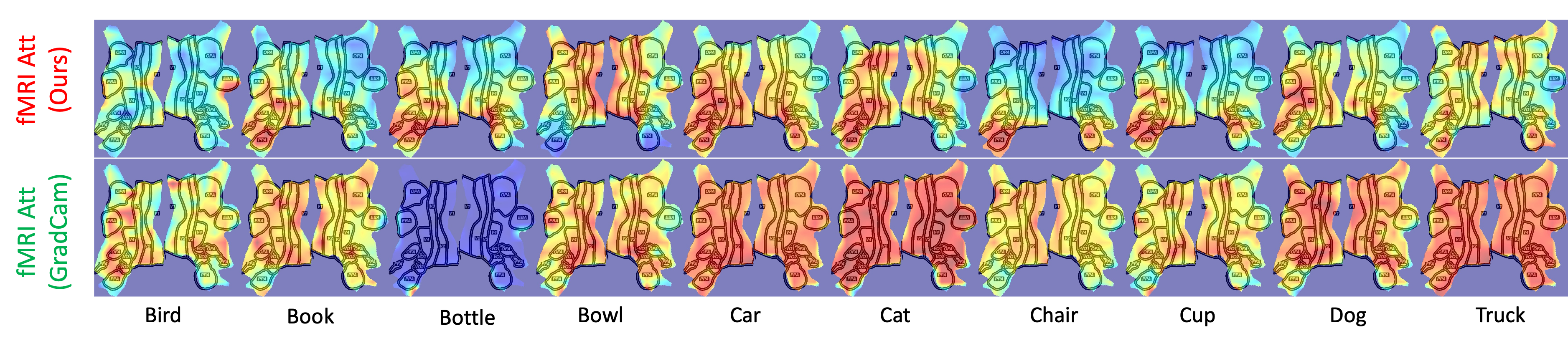
Figure 5: Average ROIs of the non-human subjects perceived by participant P1.

We illustrate the brain region attention of the human subject as in Fig. 4. The first row displays the visual stimulus, while the second row illustrates the corresponding brain activities that are a 2d version of the fMRI signal. The third row shows the visual attention map, which contains similarity scores between the SOI features and each image patch. Likewise, the fourth row displays the attention map for the SOI features in relation to each patch of brain activities. The final row is the attention map generated by GradCam [67].

Our analysis yielded two principal observations. Firstly, the attention map of the visual SOI features prominently focuses on the human figure within the visual stimulus. The visual attention map shares the same role as the fMRI attention map because they are generated by the same algorithm. Therefore, the fMRI attention map also shows the right ROI potentially. Secondly, detected ROIs show a consistent form across different visual stimuli. In particular, most attention scores are highly activated in OFA, PPA, OFA, and FFA regions that respond to the human face and body processing.

7.2 Non-Human Subjects

We illustrate the average attention maps generated by our method and GradCam of non-human subjects as in Fig. 5. The key finding is that: Our approach generates different attention maps of different subjects, making reasonable insights for the neuroscientists. Indeed, the GradCam [67] generates similar attention maps for car, cat, dog, and truck subjects, while it also could not determine ROIs for bottles.

8 Conclusion, Limitations and Broader Impacts

This paper introduces the new BRACTIVE framework to automatically localize the visual brain region of interest. The experimental results demonstrate that the ROIs w.r.t human subjects found by BRACTIVE are highly correlated with the pre-defined ROIs from neuroscience. In addition, BRACTIVE shows its superiority by determining ROIs from various non-human subjects. This ability provides reasonable references for neuroscience fields for further discovering the human brain. Finally, BRACTIVE promises a step forward in human-like learning by leveraging brain activities to guide the DNNs, making less effort on data collection and higher performance gain.

Limitations. In our proposed method, the text is leveraged to describe the context of the visual stimulus. There is a possibility that this description does not contain the subject that the participant is focusing on. There is also a case where the participant was distracted during the experiments, making recorded fMRI signals not reflect the context of the visual stimulus.

Future Work & Broader Impacts. We plan to address the limitations above and extend the BRACTIVE to different brain functionalities such as language processing, emotions, etc. More importantly, BRACTIVE promises to be a reference tool for neuroscientists and support them to debug the brain functions. With a deeper understanding of how the brain works, further novel DNNs will be inspired by these findings, boosting the AI field.

Appendix A Appendix / supplemental material

A.1 Brain Region of Interest

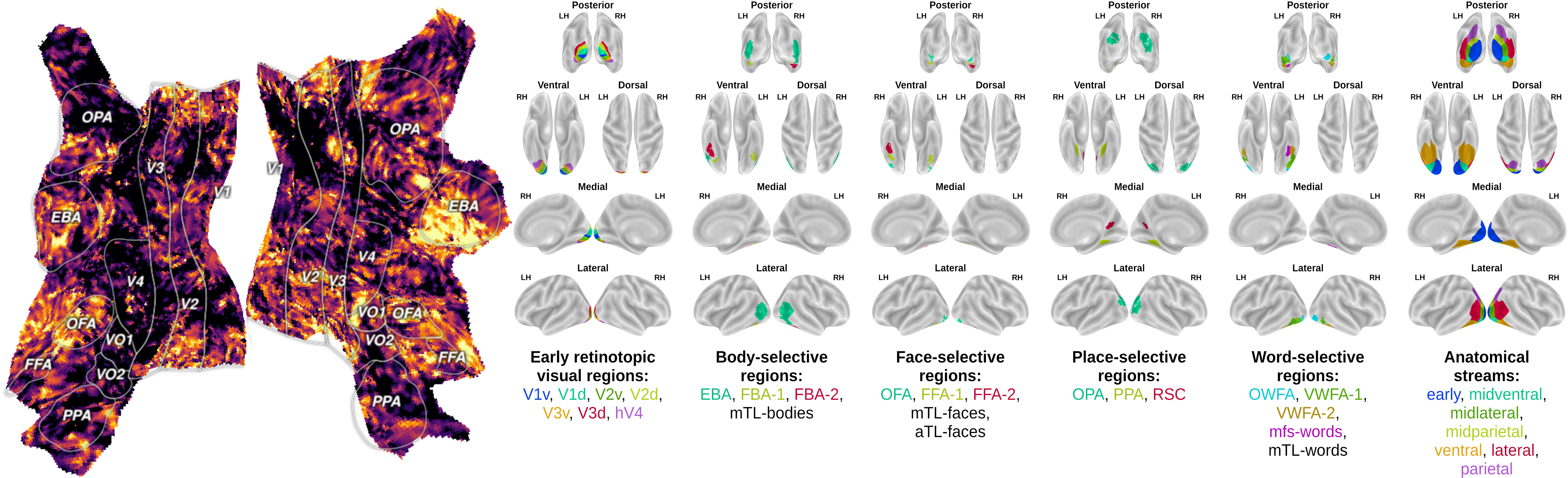
Figure 6: Brain Region of Interest (ROI)

This section briefly introduces known visual brain ROIs. We take predefined ROIs from NSD [1]. Each ROI holds a function inside the brain. According to the neuroscience findings, the functions of the ROIs can be described as:

• Early retinotopic visual regions (prf-visualrois): V1v, V1d, V2v, V2d, V3v, V3d, hV4.

• Body-selective regions (floc-bodies): EBA, FBA-1, FBA-2, mTL-bodies.

• Face-selective regions (floc-faces): OFA, FFA-1, FFA-2, mTL-faces, aTL-faces.

• Place-selective regions (floc-places): OPA, PPA, RSC.

• Word-selective regions (floc-words): OWFA, VWFA-1, VWFA-2, mfs-words, mTL-words.

• Anatomical streams (streams): early, midventral, midlateral, midparietal, ventral, lateral, parietal.

It is obvious that floc-bodies and floc-faces are related to the human subject processing. For that reason, in the experiment, we merge these ROIs in order to represent the human. The location of ROIs can be found in Fig. 6

A.2 fMRI Signals Processing

We use the official GLMsingle beta3 preparation of the data. This pipeline involves motion correlation, selection of hemodynamic response functions (HRF) for individual voxels, estimation of nuisance regressors via PCA, and subsequent fitting of a general linear model (GLM) independently for each voxel, using the selected HRF and nuisance regressor.

Additionally, we applied session-wise z-score normalization independently to each voxel, augmenting the officially released preprocessing steps. The data were processed using the FreeSurfer average brain surface space. This space encompasses a total of 327,684 vertices across the entire cerebral cortex and subcortical regions. However, for our analysis, we focused solely on 37,984 vertices within the visual cortex as defined by the nsdgeneral region of interest. The coordinates of these vertices were referenced in the inflated brain surface space.

A.3 2D Flatten of fMRI Signals

Since from NSD database [1], the fMRI signals $f\in\mathbb{R}^{N_{f}}$ are given in a float array where each element is a voxel response. This representation raises a problem: The consecutive sub-signals $\left[f_{i},f_{i+1},\dots,f_{i+t}\right],\quad t\geq 1$ does not mean that the corresponding voxels are neighbors. To prove it, we select the first 1000 elements in the given fMRI signals and project them into flattened 2D space. The Fig. 7 demonstrates that these corresponding voxels are not neighbors. Instead, they are distributed into different ROIs. For that reason, applying the typical techniques from signal processing such as Conv1D, MFCC, etc is unreasonable since these techniques discover the correlation between two voxels that are not the neighbors.

To address this issue, we propose to project all the voxel responses to flattened 2D space. This projecting function can be found from fsaverage surface. This function is also supported by Pycortex library.

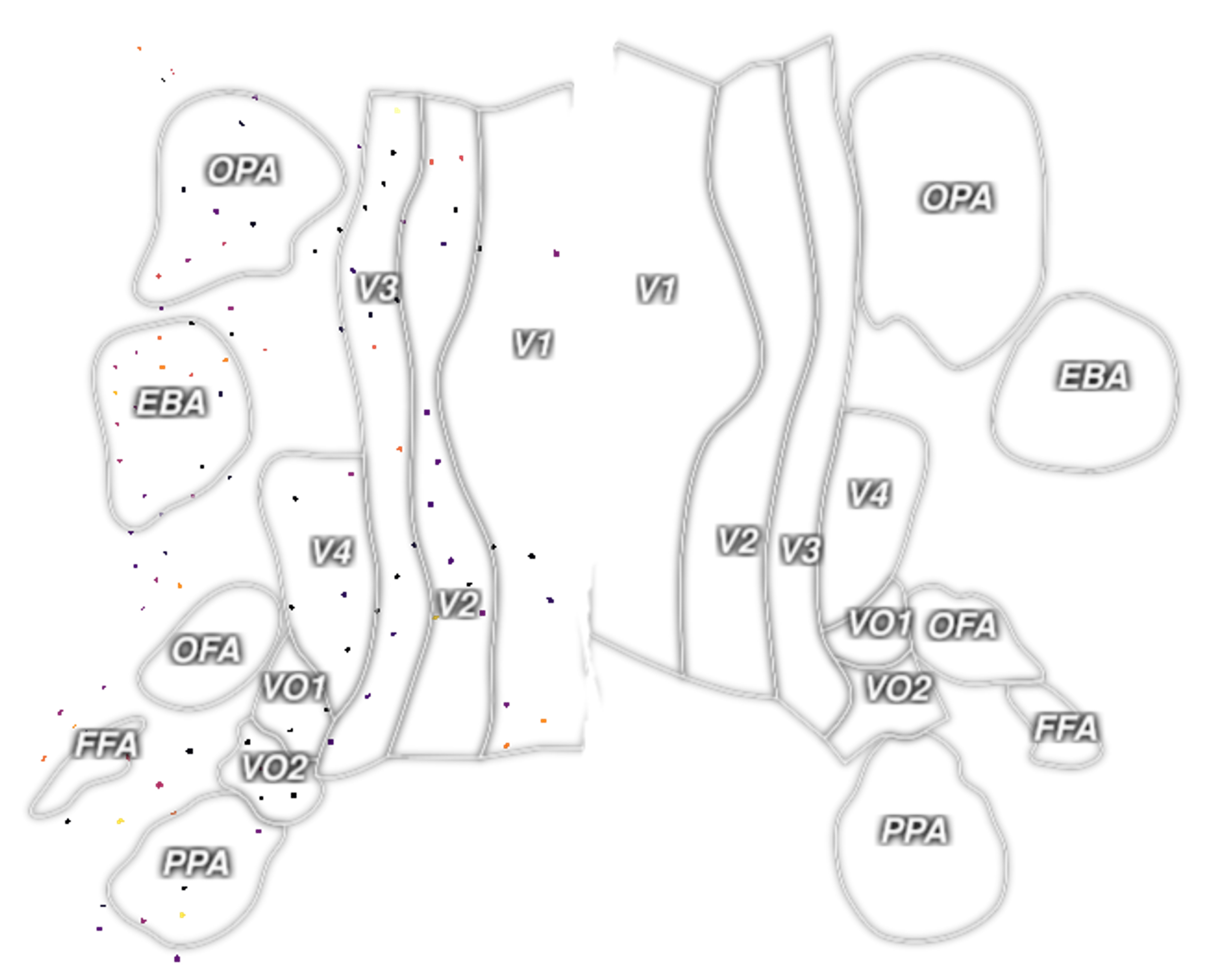
Figure 7: The first 1000 voxel responses visualized in the flattened 2D space.

A.4 Triple Contrastive Loss

The TripContras stands for triple constrastive loss function.

$$\texttt{TripContras}(\textbf{T}_{s_{k}},\textbf{P}_{s_{k}},\textbf{F}_{s_{k}})=\texttt{Contras}(\textbf{T}_{s_{k}},\textbf{P}_{s_{k}})+\texttt{Contras}(\textbf{P}_{s_{k}},\textbf{F}_{s_{k}})+\texttt{Contras}(\textbf{T}_{s_{k}},\textbf{F}_{s_{k}})$$ (9)

A.5 ROI Mask w.r.t Human Subject

This section provides additional information to the Section 6.1. We illustrate the ROI mask of the human subject as in Fig 8. The ROI masks are constructed by applying a threshold, i.e., 0.5 to the attention map. The last column is the ground truth mask which shows the brain activations of the floc-bodies and floc-faces ROI. The $6^{th}$ column is the ROI mask of our proposed method while the $7^{th}$ column is the ROI mask of GradCam [67]. We measure the dice score between the predicted masks and the corresponding ground truth. The performance is reported in the Table 1

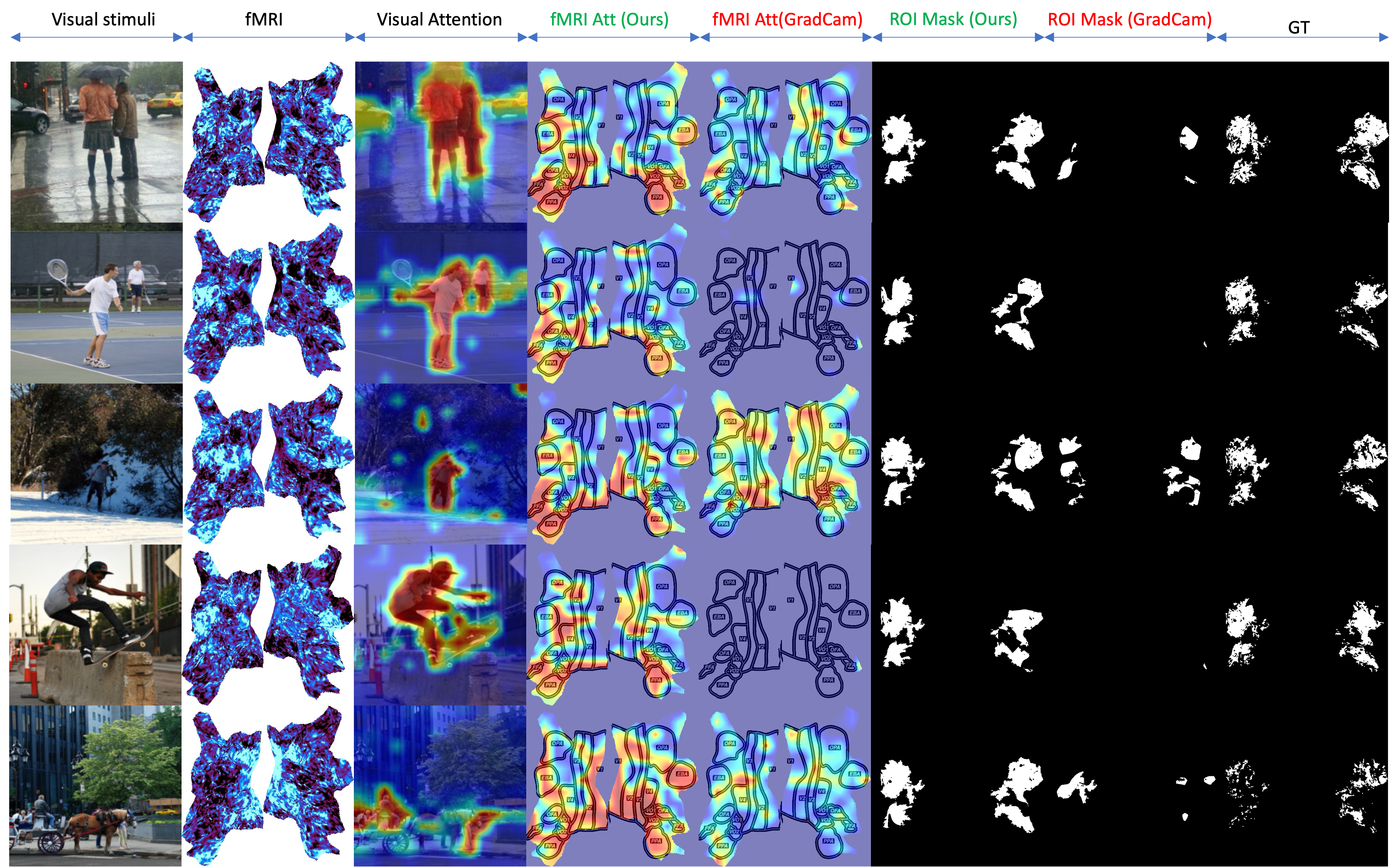
Figure 8: ROI Mask w.r.t Human. The mask is generated by applying 0.5 of the threshold to the attention maps. The $6^{th}$ and $7^{th}$ columns are the ROI masks of our method and GradCam, respectively. The last column is the ground truth of ROIs w.r.t human.

A.6 ROI w.r.t Non-human Subjects

We illustrate the ROIs of non-human subjects in Fig 9. Two key findings emerge from our observations. First, the visual attention maps generated by our method are well-fitted to the subjects. Second, compared to GradCam, our method localizes the ROIs more efficiently. For instance, with bird and bottle subjects within the visual stimulus, GradCam appears to have failed in detecting the ROIs, whereas our method succeeds.

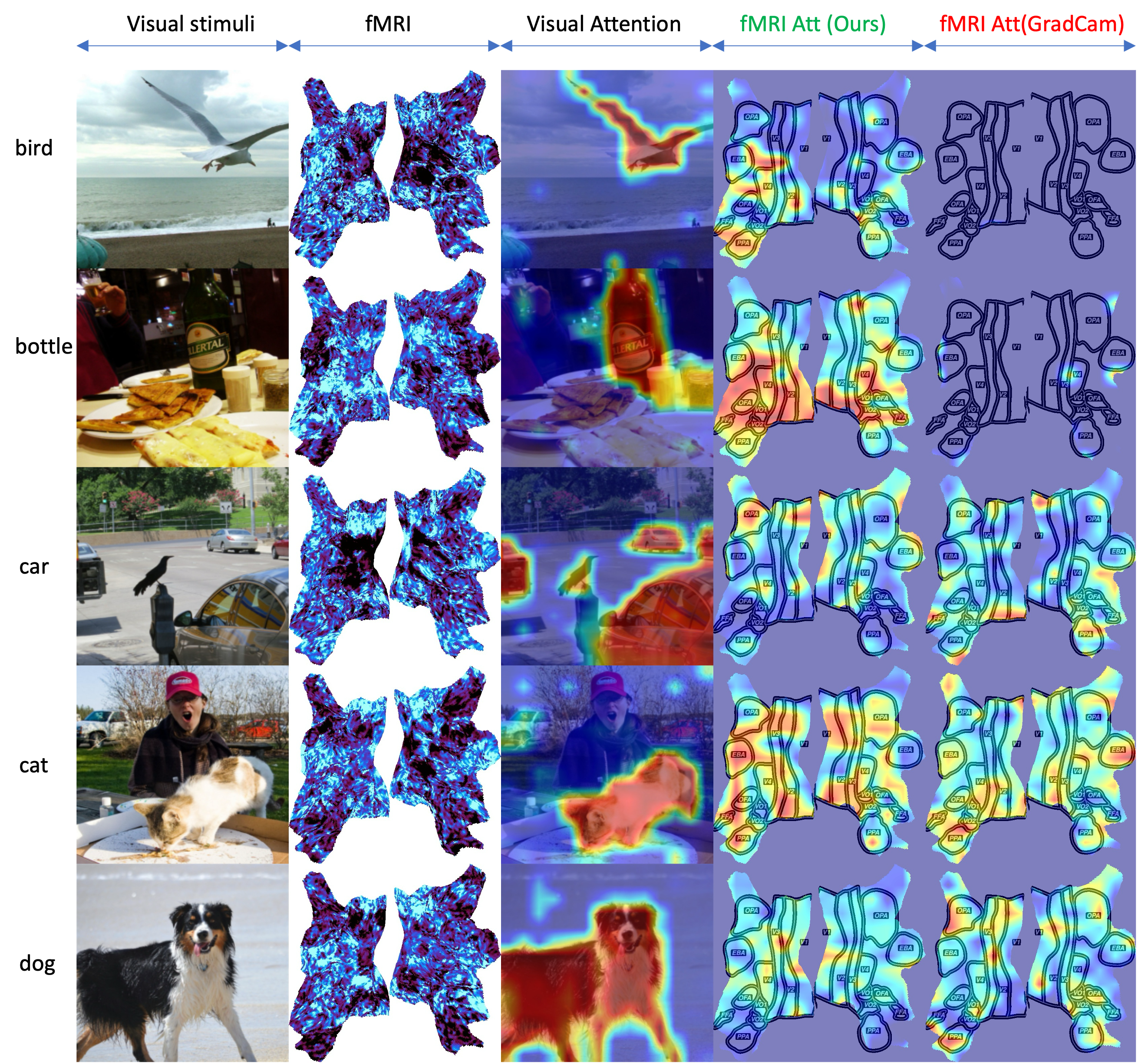
Figure 9: ROI w.r.t Non-human.

References

- [1] E. J. Allen, G. St-Yves, Y. Wu, J. L. Breedlove, J. S. Prince, L. T. Dowdle, M. Nau, B. Caron, F. Pestilli, I. Charest, et al. A massive 7t fmri dataset to bridge cognitive neuroscience and artificial intelligence. Nature neuroscience, 25(1):116–126, 2022.
- [2] E. J. Allen, G. St-Yves, Y. Wu, J. L. Breedlove, J. S. Prince, L. T. Dowdle, M. Nau, B. Caron, F. Pestilli, I. Charest, et al. A massive 7t fmri dataset to bridge cognitive neuroscience and artificial intelligence. Nature neuroscience, 25(1):116–126, 2022.
- [3] R. Anantharaman, M. Velazquez, and Y. Lee. Utilizing mask r-cnn for detection and segmentation of oral diseases. In 2018 IEEE international conference on bioinformatics and biomedicine (BIBM), pages 2197–2204. IEEE, 2018.
- [4] P. Bao, L. She, M. McGill, and D. Y. Tsao. A map of object space in primate inferotemporal cortex. Nature, 583(7814):103–108, 2020.
- [5] P. Bashivan, K. Kar, and J. J. DiCarlo. Neural population control via deep image synthesis. Science, 364(6439):eaav9436, 2019.
- [6] K. Chen, J. Wang, J. Pang, Y. Cao, Y. Xiong, X. Li, S. Sun, W. Feng, Z. Liu, J. Xu, Z. Zhang, D. Cheng, C. Zhu, T. Cheng, Q. Zhao, B. Li, X. Lu, R. Zhu, Y. Wu, J. Dai, J. Wang, J. Shi, W. Ouyang, C. C. Loy, and D. Lin. MMDetection: Open mmlab detection toolbox and benchmark. arXiv preprint arXiv:1906.07155, 2019.
- [7] Z. Chen, J. Qing, T. Xiang, W. L. Yue, and J. H. Zhou. Seeing beyond the brain: Conditional diffusion model with sparse masked modeling for vision decoding. In Proceedings of the IEEE/CVF Conference on Computer Vision and Pattern Recognition, pages 22710–22720, 2023.
- [8] R. M. Cichy, A. Khosla, D. Pantazis, A. Torralba, and A. Oliva. Comparison of deep neural networks to spatio-temporal cortical dynamics of human visual object recognition reveals hierarchical correspondence. Sci Rep, 6:27755, 06 2016.
- [9] R. M. Cichy, A. Khosla, D. Pantazis, A. Torralba, and A. Oliva. Comparison of deep neural networks to spatio-temporal cortical dynamics of human visual object recognition reveals hierarchical correspondence. Scientific reports, 6(1):27755, 2016.
- [10] I. T. Cortex. Fast readout of object identity from macaque. science, 1117593(863):310, 2005.
- [11] D. D. Cox and R. L. Savoy. Functional magnetic resonance imaging (fmri)“brain reading”: detecting and classifying distributed patterns of fmri activity in human visual cortex. Neuroimage, 19(2):261–270, 2003.
- [12] J. Cui and J. Liang. Fuzzy learning machine. Advances in Neural Information Processing Systems, 35:36693–36705, 2022.
- [13] J. Dapello, T. Marques, M. Schrimpf, F. Geiger, D. Cox, and J. J. DiCarlo. Simulating a primary visual cortex at the front of cnns improves robustness to image perturbations. Advances in Neural Information Processing Systems, 33:13073–13087, 2020.
- [14] J. Deng, W. Dong, R. Socher, L.-J. Li, K. Li, and L. Fei-Fei. Imagenet: A large-scale hierarchical image database. In 2009 IEEE conference on computer vision and pattern recognition, pages 248–255. Ieee, 2009.
- [15] J. Devlin, M.-W. Chang, K. Lee, and K. Toutanova. Bert: Pre-training of deep bidirectional transformers for language understanding. arXiv preprint arXiv:1810.04805, 2018.
- [16] A. Dosovitskiy, L. Beyer, A. Kolesnikov, D. Weissenborn, X. Zhai, T. Unterthiner, M. Dehghani, M. Minderer, G. Heigold, S. Gelly, et al. An image is worth 16x16 words: Transformers for image recognition at scale. arXiv preprint arXiv:2010.11929, 2020.
- [17] Z. Duan, Z. Lv, C. Wang, B. Chen, B. An, and M. Zhou. Few-shot generation via recalling brain-inspired episodic-semantic memory. Advances in Neural Information Processing Systems, 36, 2024.
- [18] R. C. Fong, W. J. Scheirer, and D. D. Cox. Using human brain activity to guide machine learning. Scientific reports, 8(1):5397, 2018.
- [19] R. C. Fong, W. J. Scheirer, and D. D. Cox. Using human brain activity to guide machine learning. Scientific reports, 8(1):5397, 2018.
- [20] A. T. Gifford, B. Lahner, S. Saba-Sadiya, M. G. Vilas, A. Lascelles, A. Oliva, K. Kay, G. Roig, and R. M. Cichy. The algonauts project 2023 challenge: How the human brain makes sense of natural scenes. arXiv preprint arXiv:2301.03198, 2023.
- [21] A. Graves, G. Wayne, M. Reynolds, T. Harley, I. Danihelka, A. Grabska-Barwińska, S. G. Colmenarejo, E. Grefenstette, T. Ramalho, J. Agapiou, et al. Hybrid computing using a neural network with dynamic external memory. Nature, 538(7626):471–476, 2016.
- [22] K. Gregor, I. Danihelka, A. Graves, D. Rezende, and D. Wierstra. Draw: A recurrent neural network for image generation. In International conference on machine learning, pages 1462–1471. PMLR, 2015.
- [23] U. Güçlü and M. A. Van Gerven. Deep neural networks reveal a gradient in the complexity of neural representations across the ventral stream. Journal of Neuroscience, 35(27):10005–10014, 2015.
- [24] J. V. Haxby, M. I. Gobbini, M. L. Furey, A. Ishai, J. L. Schouten, and P. Pietrini. Distributed and overlapping representations of faces and objects in ventral temporal cortex. Science, 293(5539):2425–2430, 2001.
- [25] J.-D. Haynes and G. Rees. Predicting the orientation of invisible stimuli from activity in human primary visual cortex. Nature neuroscience, 8(5):686–691, 2005.
- [26] T. Horikawa and Y. Kamitani. Generic decoding of seen and imagined objects using hierarchical visual features. Nat Commun, 8:15037, May 2017.
- [27] Y. Kamitani and F. Tong. Decoding the visual and subjective contents of the human brain. Nature neuroscience, 8(5):679–685, 2005.
- [28] X. Kan, W. Dai, H. Cui, Z. Zhang, Y. Guo, and C. Yang. Brain network transformer. Advances in Neural Information Processing Systems, 35:25586–25599, 2022.
- [29] M. Khosla, K. Jamison, A. Kuceyeski, and M. Sabuncu. Characterizing the ventral visual stream with response-optimized neural encoding models. Advances in Neural Information Processing Systems, 35:9389–9402, 2022.
- [30] P. Y. Kim, J. Kwon, S. Joo, S. Bae, D. Lee, Y. Jung, S. Yoo, J. Cha, and T. Moon. Swift: Swin 4d fmri transformer. arXiv preprint arXiv:2307.05916, 2023.
- [31] N. Kriegeskorte, M. Mur, and P. A. Bandettini. Representational similarity analysis-connecting the branches of systems neuroscience. Frontiers in systems neuroscience, 2:249, 2008.
- [32] C. Lee, J. Han, M. Feilong, G. Jiahui, J. Haxby, and C. Baldassano. Hyper-hmm: aligning human brains and semantic features in a common latent event space. Advances in Neural Information Processing Systems, 36, 2024.
- [33] S. Lin, T. Sprague, and A. K. Singh. Mind reader: Reconstructing complex images from brain activities. Advances in Neural Information Processing Systems, 35:29624–29636, 2022.
- [34] T.-Y. Lin, M. Maire, S. Belongie, J. Hays, P. Perona, D. Ramanan, P. Dollár, and C. L. Zitnick. Microsoft coco: Common objects in context. In Computer Vision–ECCV 2014: 13th European Conference, Zurich, Switzerland, September 6-12, 2014, Proceedings, Part V 13, pages 740–755. Springer, 2014.
- [35] D. Liu, W. Dai, H. Zhang, X. Jin, J. Cao, and W. Kong. Brain-machine coupled learning method for facial emotion recognition. IEEE Transactions on Pattern Analysis and Machine Intelligence, 45(9):10703–10717, 2023.
- [36] Y. Liu, M. Ott, N. Goyal, J. Du, M. Joshi, D. Chen, O. Levy, M. Lewis, L. Zettlemoyer, and V. Stoyanov. Roberta: A robustly optimized bert pretraining approach. arXiv preprint arXiv:1907.11692, 2019.
- [37] I. Loshchilov and F. Hutter. Sgdr: Stochastic gradient descent with warm restarts. arXiv preprint arXiv:1608.03983, 2016.
- [38] I. Loshchilov and F. Hutter. Decoupled weight decay regularization. arXiv preprint arXiv:1711.05101, 2017.
- [39] J. Millet, C. Caucheteux, Y. Boubenec, A. Gramfort, E. Dunbar, C. Pallier, J.-R. King, et al. Toward a realistic model of speech processing in the brain with self-supervised learning. Advances in Neural Information Processing Systems, 35:33428–33443, 2022.
- [40] M. C. Nechyba and Y. Xu. Human skill transfer: neural networks as learners and teachers. In Proceedings 1995 IEEE/RSJ International Conference on Intelligent Robots and Systems. Human Robot Interaction and Cooperative Robots, volume 3, pages 314–319. IEEE, 1995.
- [41] H.-Q. Nguyen, T.-D. Truong, X. B. Nguyen, A. Dowling, X. Li, and K. Luu. Insect-foundation: A foundation model and large-scale 1m dataset for visual insect understanding. arXiv preprint arXiv:2311.15206, 2023.
- [42] P. Nguyen, K. G. Quach, C. N. Duong, N. Le, X.-B. Nguyen, and K. Luu. Multi-camera multiple 3d object tracking on the move for autonomous vehicles. In Proceedings of the IEEE/CVF Conference on Computer Vision and Pattern Recognition, pages 2569–2578, 2022.
- [43] X. B. Nguyen, A. Bisht, H. Churchill, and K. Luu. Two-dimensional quantum material identification via self-attention and soft-labeling in deep learning. arXiv preprint arXiv:2205.15948, 2022.
- [44] X.-B. Nguyen, D. T. Bui, C. N. Duong, T. D. Bui, and K. Luu. Clusformer: A transformer based clustering approach to unsupervised large-scale face and visual landmark recognition. In Proceedings of the IEEE/CVF conference on computer vision and pattern recognition, pages 10847–10856, 2021.
- [45] X.-B. Nguyen, C. N. Duong, X. Li, S. Gauch, H.-S. Seo, and K. Luu. Micron-bert: Bert-based facial micro-expression recognition. In Proceedings of the IEEE/CVF Conference on Computer Vision and Pattern Recognition, pages 1482–1492, 2023.
- [46] X.-B. Nguyen, C. N. Duong, M. Savvides, K. Roy, H. Churchill, and K. Luu. Fairness in visual clustering: A novel transformer clustering approach. arXiv preprint arXiv:2304.07408, 2023.
- [47] X.-B. Nguyen, G.-S. Lee, S.-H. Kim, and H.-J. Yang. Audio-video based emotion recognition using minimum cost flow algorithm. In 2019 IEEE/CVF International Conference on Computer Vision Workshop (ICCVW), pages 3737–3741. IEEE, 2019.
- [48] X.-B. Nguyen, G. S. Lee, S. H. Kim, and H. J. Yang. Self-supervised learning based on spatial awareness for medical image analysis. IEEE Access, 8:162973–162981, 2020.
- [49] X.-B. Nguyen, X. Li, S. U. Khan, and K. Luu. Brainformer: Modeling mri brain functions to machine vision. arXiv preprint arXiv:2312.00236, 2023.
- [50] X.-B. Nguyen, X. Liu, X. Li, and K. Luu. The algonauts project 2023 challenge: Uark-ualbany team solution. arXiv preprint arXiv:2308.00262, 2023.
- [51] B. Nguyen-Xuan and G.-S. Lee. Sketch recognition using lstm with attention mechanism and minimum cost flow algorithm. International Journal of Contents, 15(4):8–15, 2019.
- [52] S. Nishida, Y. Nakano, A. Blanc, N. Maeda, M. Kado, and S. Nishimoto. Brain-mediated transfer learning of convolutional neural networks. In Proceedings of the AAAI Conference on Artificial Intelligence, volume 34, pages 5281–5288, 2020.
- [53] S. Nishimoto, A. T. Vu, T. Naselaris, Y. Benjamini, B. Yu, and J. L. Gallant. Reconstructing visual experiences from brain activity evoked by natural movies. Curr. Biol., 21(19):1641–1646, Oct 2011.
- [54] F. Ozcelik and R. VanRullen. Brain-diffuser: Natural scene reconstruction from fmri signals using generative latent diffusion. arXiv preprint arXiv:2303.05334, 2023.
- [55] F. Ozcelik and R. VanRullen. Natural scene reconstruction from fmri signals using generative latent diffusion. Scientific Reports, 13(1):15666, 2023.
- [56] S. Palazzo, C. Spampinato, I. Kavasidis, D. Giordano, J. Schmidt, and M. Shah. Decoding brain representations by multimodal learning of neural activity and visual features. IEEE Transactions on Pattern Analysis and Machine Intelligence, 43(11):3833–3849, 2020.
- [57] S. Palazzo, C. Spampinato, I. Kavasidis, D. Giordano, and M. Shah. Generative adversarial networks conditioned by brain signals. In ICCV, pages 3430–3438, Oct 2017.
- [58] J. W. Peirce. Understanding mid-level representations in visual processing. Journal of Vision, 15(7):5–5, 2015.
- [59] G. Pogoncheff, J. Granley, and M. Beyeler. Explaining v1 properties with a biologically constrained deep learning architecture. Advances in Neural Information Processing Systems, 36:13908–13930, 2023.
- [60] C. R. Ponce, W. Xiao, P. F. Schade, T. S. Hartmann, G. Kreiman, and M. S. Livingstone. Evolving images for visual neurons using a deep generative network reveals coding principles and neuronal preferences. Cell, 177(4):999–1009, 2019.
- [61] J. Portes, C. Schmid, and J. M. Murray. Distinguishing learning rules with brain machine interfaces. Advances in neural information processing systems, 35:25937–25950, 2022.
- [62] J. Quesada, L. Sathidevi, R. Liu, N. Ahad, J. Jackson, M. Azabou, J. Xiao, C. Liding, M. Jin, C. Urzay, et al. Mtneuro: A benchmark for evaluating representations of brain structure across multiple levels of abstraction. Advances in neural information processing systems, 35:5299–5314, 2022.
- [63] A. Radford, J. W. Kim, C. Hallacy, A. Ramesh, G. Goh, S. Agarwal, G. Sastry, A. Askell, P. Mishkin, J. Clark, et al. Learning transferable visual models from natural language supervision. In International conference on machine learning, pages 8748–8763. PMLR, 2021.
- [64] S. Safarani, A. Nix, K. Willeke, S. Cadena, K. Restivo, G. Denfield, A. Tolias, and F. Sinz. Towards robust vision by multi-task learning on monkey visual cortex. Advances in Neural Information Processing Systems, 34:739–751, 2021.
- [65] G. H. Sarch, M. J. Tarr, K. Fragkiadaki, and L. Wehbe. Brain dissection: fmri-trained networks reveal spatial selectivity in the processing of natural images. bioRxiv, pages 2023–05, 2023.
- [66] P. S. Scotti, A. Banerjee, J. Goode, S. Shabalin, A. Nguyen, E. Cohen, A. J. Dempster, N. Verlinde, E. Yundler, D. Weisberg, et al. Reconstructing the mind’s eye: fmri-to-image with contrastive learning and diffusion priors. arXiv preprint arXiv:2305.18274, 2023.
- [67] R. R. Selvaraju, M. Cogswell, A. Das, R. Vedantam, D. Parikh, and D. Batra. Grad-cam: Visual explanations from deep networks via gradient-based localization. In Proceedings of the IEEE international conference on computer vision, pages 618–626, 2017.
- [68] M. Serna-Aguilera, X. B. Nguyen, A. Singh, L. Rockers, S.-W. Park, L. Neely, H.-S. Seo, and K. Luu. Video-based autism detection with deep learning. In 2024 IEEE Green Technologies Conference (GreenTech), pages 159–161. IEEE, 2024.
- [69] K. J. Seymour, M. A. Williams, and A. N. Rich. The representation of color across the human visual cortex: distinguishing chromatic signals contributing to object form versus surface color. Cerebral cortex, 26(5):1997–2005, 2016.
- [70] C. Spampinato, S. Palazzo, I. Kavasidis, D. Giordano, N. Souly, and M. Shah. Deep Learning Human Mind for Automated Visual Classification. In CVPR, pages 4503–4511, jul 2017.
- [71] D. E. Stansbury, T. Naselaris, and J. L. Gallant. Natural scene statistics account for the representation of scene categories in human visual cortex. Neuron, 79(5):1025–1034, Sep 2013.
- [72] Y. Takagi and S. Nishimoto. High-resolution image reconstruction with latent diffusion models from human brain activity. In Proceedings of the IEEE/CVF Conference on Computer Vision and Pattern Recognition, pages 14453–14463, 2023.
- [73] B. Thirion, E. Duchesnay, E. Hubbard, J. Dubois, J.-B. Poline, D. Lebihan, and S. Dehaene. Inverse retinotopy: inferring the visual content of images from brain activation patterns. Neuroimage, 33(4):1104–1116, 2006.
- [74] A. Thomas, C. Ré, and R. Poldrack. Self-supervised learning of brain dynamics from broad neuroimaging data. Advances in neural information processing systems, 35:21255–21269, 2022.
- [75] A. Thual, Q. H. Tran, T. Zemskova, N. Courty, R. Flamary, S. Dehaene, and B. Thirion. Aligning individual brains with fused unbalanced gromov wasserstein. Advances in neural information processing systems, 35:21792–21804, 2022.
- [76] T.-D. Truong, R. T. N. Chappa, X.-B. Nguyen, N. Le, A. P. Dowling, and K. Luu. Otadapt: Optimal transport-based approach for unsupervised domain adaptation. In 2022 26th international conference on pattern recognition (ICPR), pages 2850–2856. IEEE, 2022.
- [77] T. Xiao, Y. Liu, B. Zhou, Y. Jiang, and J. Sun. Unified perceptual parsing for scene understanding. In Proceedings of the European conference on computer vision (ECCV), pages 418–434, 2018.
- [78] K. Xu, J. Ba, R. Kiros, K. Cho, A. Courville, R. Salakhudinov, R. Zemel, and Y. Bengio. Show, attend and tell: Neural image caption generation with visual attention. In International conference on machine learning, pages 2048–2057. PMLR, 2015.
- [79] D. L. Yamins, H. Hong, C. Cadieu, and J. J. DiCarlo. Hierarchical modular optimization of convolutional networks achieves representations similar to macaque it and human ventral stream. Advances in neural information processing systems, 26, 2013.
- [80] D. L. Yamins, H. Hong, C. F. Cadieu, E. A. Solomon, D. Seibert, and J. J. DiCarlo. Performance-optimized hierarchical models predict neural responses in higher visual cortex. Proceedings of the national academy of sciences, 111(23):8619–8624, 2014.
- [81] D. L. Yamins, H. Hong, C. F. Cadieu, E. A. Solomon, D. Seibert, and J. J. DiCarlo. Performance-optimized hierarchical models predict neural responses in higher visual cortex. Proceedings of the national academy of sciences, 111(23):8619–8624, 2014.
- [82] B. Zhou, H. Zhao, X. Puig, S. Fidler, A. Barriuso, and A. Torralba. Scene parsing through ade20k dataset. In Proceedings of the IEEE Conference on Computer Vision and Pattern Recognition, 2017.