Fast Explainability via Feasible Concept Sets Generator

Abstract

A long-standing dilemma prevents the broader application of explanation methods: general applicability and inference speed. On the one hand, existing model-agnostic explanation methods usually make minimal pre-assumptions about the prediction models to be explained. Still, they require additional queries to the model through propagation or back-propagation to approximate the models’ behaviors, resulting in slow inference and hindering their use in time-sensitive tasks. On the other hand, various model-dependent explanations have been proposed that achieve low-cost, fast inference but at the expense of limiting their applicability to specific model structures. In this study, we bridge the gap between the universality of model-agnostic approaches and the efficiency of model-specific approaches by proposing a novel framework without assumptions on the prediction model’s structures, achieving high efficiency during inference and allowing for real-time explanations. To achieve this, we first define explanations through a set of human-comprehensible concepts and propose a framework to elucidate model predictions via minimal feasible concept sets. Second, we show that a minimal feasible set generator can be learned as a companion explainer to the prediction model, generating explanations for predictions. Finally, we validate this framework by implementing a novel model-agnostic method that provides robust explanations while facilitating real-time inference. Our claims are substantiated by comprehensive experiments, highlighting the effectiveness and efficiency of our approach.

1 Introduction

The increasing complexity and opacity of deep machine learning models have created significant challenges in ensuring their broad application, particularly in high-stakes domains where model transparency and safety are paramount. Various research has been conducted to address these concerns [1, 2, 3]. While deep models demonstrate superior performance across various tasks, their “black-box” nature often impedes their acceptance and deployment in critical areas such as healthcare, finance, and autonomous systems [4, 5, 6, 7, 8]. In these contexts, it is essential not only to achieve high predictive accuracy but also to provide clear, understandable explanations of the models’ decisions.

Many explanation methods have been developed to mitigate the opacity inherent in deep machine learning models. Despite their potential, the application of these explanation methods remains minimal compared to the extensive deployment of deep models in real-world scenarios. The concept of explainability is scarcely realized in practical applications, a situation that potentially stems from the difficulty of balancing general applicability with inference speed. It is a long-standing dilemma in explainable artificial intelligence (XAI), as both are crucial for large-scale deployment.

Model-specific methods leverage by-products of prediction models, such as gradients, feature maps, and attention weights, to facilitate rapid interpretations. However, they are often restricted to specific network architectures, like CNNs [9] and Transformers [10, 11]. On the other hand, model-agnostic approaches [12, 13, 14, 15] can accommodate a wider range of model types but typically require extensive fitting processes or iterative gradient calculations, making them impractical for real-world applications due to their high computational costs.

In recent developments, various explanation methods have been proposed; however, they each tend to address only one aspect of the dilemma – either general applicability or rapid inference – without successfully reconciling both. Model-specific methods, which utilize by-products of the prediction models such as gradients, feature maps, and attention weights, can deliver fast interpretations but are usually limited to specific types of network structures, such as CNNs [9] and Transformers [10, 11]. In contrast, model-agnostic methods [12, 13, 14, 15] can interpret a broader range of models but typically require additional fitting processes or repetitive gradient calculations, hindering their real-world applications due to cost inefficiency. In this study, we aim to bridge the gap between model restrictions and inference speed by developing a framework to learn an explanation companion model capable of inferring explanations in real time for any machine learning model.

We summarize our contributions as follows: 1) We define explanations through a set of human-comprehensible concepts, which can be tailored to match the users’ level of understanding, ensuring that explanations are accessible and meaningful to diverse audiences; 2) We propose a framework for learning the generators for the minimal feasible concept sets, which serves as a companion explainer for the prediction model, and ensures fast inference; 3) We validate the effectiveness of this framework by developing and implementing a versatile model-agnostic method applicable to both image and text classification tasks. This method learns explainers that generate explanations efficiently, demonstrating the framework’s practical utility and adaptability.

2 Related Work

In this section, we review two types of explanation approaches: 1) model-agnostic approaches, which are independent of specific model structures, and 2) model-specific approaches, which are usually optimized for specific model structures for efficient inference.

Model-agnostic approaches: Model-agnostic approaches are designed to be broadly applicable, making minimal or no assumptions about the prediction models to be explained. One common strategy involves using surrogates to approximate the local behavior of models, which is particularly useful for black-box models. For instance, LIME [12] fits a surrogate interpretable model (such as a linear model) to explain predictions locally by perturbing the input data and observing the changes in predictions. Similarly, SHAP [13] leverages Shapley values from game theory to ensure a unique surrogate solution with desirable properties such as local accuracy, missingness, and consistency. RISE [14] generates saliency maps by sampling randomized masks and evaluating their impact on the model’s output, sharing the idea of surrogate fitting via random input perturbation like LIME and SHAP, but using saliency maps as local surrogates. These surrogate methods, however, are resource-intensive due to the random sampling and additional model queries required. For example, SHAP often necessitates numerous additional queries to estimate marginal distributions around a given input, resulting in significant computational overhead.

Another model-agnostic strategy involves utilizing the gradient information from white-box models. Rather than learning surrogates, these methods exploit locally smoothed gradients to approximate the local behavior of prediction models. Integrated Gradients [16], for example, smooths gradients by averaging those of interpolated samples between a baseline and a specific input. While this interpolation can be viewed as uniform sampling, AGI [17] proposes a sampling strategy that utilizes adversarial attacks to locate decision boundaries. NeFLAG [18], inspired by the divergence theorem, approximates smoothed gradients via the flux of gradients flowing over a hypersphere. Despite their effectiveness, gradient-based approaches often fail to provide efficient explanations due to the necessity of additional model queries and back-propagations.

Model-specific approaches: Model-specific approaches are typically tailored to specific model architectures, enabling fast explanations by repurposing by-products (such as attention weights and feature maps) of the prediction models’ outputs as explanatory ingredients. GradCAM [9], for instance, repurposes feature maps and uses their weighted average to generate explanations, effectively working on CNNs or Transformers. Similarly, methods like AttLRP [10] and AttCAT [11] are designed specifically for transformer-based models, relying on attention weights from various attention heads and layers to compute final explanations.

DeepLIFT [19] provides a framework for explaining deep learning models under the condition that propagation rules can be adapted. This framework requires detailed understanding and careful handling of the forward and backward passes within neural networks, limiting its applicability in complex architectures like RNNs. TreeSHAP [20], a special case of SHAP, achieves efficient explanations by leveraging the nature of tree-based models. Understanding the inner workings of specific model architectures is crucial for achieving fast inference speeds, as explanations can utilize the by-products of prediction models effectively only if the significance of these by-products is well understood.

In this study, we aim to bridge the gap between the universality of model-agnostic approaches and the efficiency of model-specific approaches. We propose an explainer learning framework that requires no assumptions about the prediction model’s structures while achieving both high time and memory efficiency, ensuring the capability for real-time explanations.

3 Proposed Method

In this section, we first introduce a definition of explainability in terms of comprehensible concepts and feasible concept sets. Then, we propose a general framework for the minimum feasible set generation method and implement a model agnostic method based on the framework with custom concept mapping functions.

3.1 Defining Explainability

Definition 1

(Comprehensible Concept and Concept Mapping Function) A concept $c$ is manually designed following certain rules, which ensures that individuals with proper background knowledge can understand the concepts. A concept mapping function maps the sample $\boldsymbol{x}$ to a concept $c$ via $c=f_{map}(\boldsymbol{x})$, denoting that $\boldsymbol{x}$ has concept $c$.

Explanations should be provided based on comprehensible concepts, which can vary depending on the context. Therefore, to generate explanations for a prediction, it is crucial first to define the concepts on which these explanations will be based.

Definition 2

(Concept Mapping Function Set) A set of concept mapping functions mapping the raw input features to a set of concepts, $\mathcal{F}_{map}:X\to C$, i.e., given one input $\boldsymbol{x}\in X$, we obtain a set of concepts $\{c_{i}=f_{map}^{i}(\boldsymbol{x})|f_{map}^{i}\in\mathcal{F}_{map}\}=C$.

Defining the concepts is equivalent to defining the set of concept mapping functions. Taking the image and text data as examples, for image data, when choosing image patches as concepts, we can express an image $\boldsymbol{x}$ as a sequence of $M$ individual patches $(p_{1},...,p_{M})$. Similarly, for text data, we can express it as a token sequence $\boldsymbol{x}$ of length $M$. In both scenarios, a concept mapping function can be defined by $f_{map}^{s}(\boldsymbol{x})=\boldsymbol{s}\odot\boldsymbol{x}$, where $\boldsymbol{s}\in\{0,1\}^{M}$ is a permutation of $\{1,0\}$ of length $M$ and the set of concept mapping functions can be written by $\mathcal{F}_{map}=\{f^{\boldsymbol{s}}_{map}|\boldsymbol{s}\in\{0,1\}^{M}\}$. The concept set then consists of all possible combinations of patches or tokens.

Definition 3

(Concept Elimination) Assume that $f_{map}^{i}$ is a concept mapping function, let $X_{0}^{i}$ denotes its null space, i.e., $f_{map}^{i}(X_{0}^{i})=0$, or equivalently $(f_{map}^{i})^{-1}(0)=X_{0}^{i}$, we define that concept $c_{i}$ is eliminated from the input $\boldsymbol{x}$ by its projection on the null space $X_{0}^{i}$. i.e.,

$$\boldsymbol{x}_{\backslash i}=P(X_{0}^{i})(\boldsymbol{x}),$$ (1)

where $P(X_{0}^{i})$ is the projection operator onto the null space $X_{0}^{i}$.

In our example setting for image or text data, given input $\boldsymbol{x}$, the null space of the concept $c_{\boldsymbol{s}}=f_{map}^{\boldsymbol{s}}(\boldsymbol{x})$ can be obtained by spanning the set $\{\boldsymbol{s}\odot\boldsymbol{x}|\boldsymbol{x}\in X,\boldsymbol{s}\odot\boldsymbol{x}=0\}$. Therefore, the projection onto the null space of concept $c_{\boldsymbol{s}}$ becomes $\boldsymbol{x}_{\backslash\boldsymbol{s}}=P(X_{0}^{\boldsymbol{s}})(\boldsymbol{x})=(\boldsymbol{1}-\boldsymbol{s})\odot\boldsymbol{x}$, where $\boldsymbol{1}-\boldsymbol{s}$ denotes the complementary of the permutation $\boldsymbol{s}$.

Definition 4

(Feasible Elimination Set) Assume we eliminate a set of concepts $C_{fe}$ via the process defined by Definition 3, we say that the concept set $C_{fe}$ is an $\epsilon$-feasible elimination set if and only if $d(f(\boldsymbol{x}),f(\boldsymbol{x}_{\backslash C_{fe}}))<\epsilon$, where $d(\cdot,\cdot)$ measures the discrepancy between the model’s two predictions, $\epsilon$ is the tolerance and $\boldsymbol{x}_{\backslash C_{fe}}$ is the corresponding projected input onto the null space $X_{0}^{(C_{fe})}$.

Definition 5

(Feasible Set) Given a set $C_{f}$, and a feasible elimination set $C_{fe}$, we have the union $C=C_{f}\cup C_{fe}$. If $C$’s null space is equal to the null space of $\{c_{i}=f_{map}^{i}(\boldsymbol{x})|f_{map}^{i}\in\mathcal{F}_{map}\}$, i.e. the set of all concepts, we call that $C_{f}$ is a feasible set.

Note that the complement of the null space $X_{0}^{(C_{fe})}$ is not necessarily $X_{0}^{(C_{f})}$.

Definition 6

(Maximum Feasible Elimination Set) Given the null space $X_{0}^{(C_{fe})}$ of a feasible elimination set $C_{fe}$, denote the cardinality of this feasible elimination set as the rank of the null space. The maximum feasible elimination set is defined by the feasible elimination set with the highest cardinality. i.e.,

$$C_{fe}^{*}=\operatorname{argmax}_{C_{fe}}\operatorname{Card}(X_{0}^{(C_{fe})})$$ (2)

Definition 7

(Minimum Feasible Set) Given the null space $X_{0}^{(C_{f})}$ of a feasible set $C_{f}$, the minimum feasible set is defined by the feasible set with the lowest cardinality. i.e.,

$$C_{f}^{*}=\operatorname{argmin}_{C_{f}}\operatorname{Card}(X_{0}^{(C_{f})})$$ (3)

This is the core of our framework for explanation. We can interpret the minimum feasible set as the minimum collection of concepts that yields the same prediction as raw input $\boldsymbol{x}$ with tolerance $\epsilon$. Hence we can explain the prediction by the concepts in this minimum feasible set. In our example setting, it’s equivalent to finding the minimum collection of patches/tokens that don’t alter the predictions.

3.2 Generating Feasible Sets

Assume we have a prediction model $y=f(\boldsymbol{x})$, and for any input $\boldsymbol{x}$, we have a set $\mathcal{F}_{map}$ of concept mapping functions , hence concept $c_{i}$ can be obtained by $c_{i}=f^{i}_{map}(\boldsymbol{x})$, where $f^{i}_{map}\in\mathcal{F}_{map}$.

Let’s define a distribution $p(\mathcal{F}_{map},\boldsymbol{x})$, from which we can generate random concept mapping functions given $\mathcal{F}_{map}$ and $\boldsymbol{x}$. From this distribution, for a specific input $\boldsymbol{x}$, we can generate a set of concepts $C_{ge}$ to be eliminated. The corresponding input projected onto the null space is denoted by $\boldsymbol{x}_{\backslash C_{g}}$. As per Definition 4, if $d(f(\boldsymbol{x}),f(\boldsymbol{x}_{\backslash C_{ge}}))<\epsilon$, then $C_{ge}$ is a feasible elimination set. To ensure any set draw from $p(\mathcal{F}_{map},\boldsymbol{x})$ is a feasible elimination set, it is intuitive to have the following condition

$$\mathbb{E}_{C_{ge}\sim p(\mathcal{F}_{map},\boldsymbol{x})}d(f(\boldsymbol{x}),f(\boldsymbol{x}_{\backslash C_{ge}}))<\epsilon$$ (4)

If, instead, we choose to generate a feasible set $C_{g}$ other than $C_{ge}$, to ensure its feasible, the condition becomes

$$\mathbb{E}_{C_{g}\sim p(\mathcal{F}_{map},\boldsymbol{x})}d(f(\boldsymbol{x}),f(\boldsymbol{x}_{C_{g}}))<\epsilon$$ (5)

3.3 Generating Minimum Feasible Sets

Referring to Definition 7, we need to constrain the cardinality of $X_{0}^{C_{g}}$, i.e., the rank of the null space of $C_{g}$, to obtain a minimum feasible set. This leads to a minimization objective

$$\min_{p}\mathbb{E}_{C_{g}\sim p(\mathcal{F}_{map},\boldsymbol{x})}\operatorname{Card}(X_{0}^{C_{g}})$$ (6)

s.t. $$\mathbb{E}_{C_{g}\sim p(\mathcal{F}_{map},\boldsymbol{x})}(d(f(\boldsymbol{x}),f(\boldsymbol{x}_{\backslash C_{g}}))-\epsilon)>0$$

the constraint can be rewritten as a multiplier term. Given proper $\lambda$, the optimization function becomes

$$\min_{p}\mathbb{E}_{C_{g}\sim p(\mathcal{F}_{map},\boldsymbol{x})}\operatorname{Card}(X_{0}^{C_{g}})+\lambda\cdot d(f(\boldsymbol{x}),f(\boldsymbol{x}_{C_{g}})),$$ (7)

where $\epsilon$ is omitted as it is a constant.

3.4 An Implementation of the Framework

Note that given different choices of concept mapping functions, a few existing methods can be categorized as special cases of this framework. For instance,

Special Case I: When defining the concept mapping functions as the feature map extractors in CNN, i.e., $f_{map}^{i}(\boldsymbol{x})=A^{(i)}$ where $f_{map}\in\mathcal{F}_{map}$ and $A^{(i)}$ is a feature map, by first-order approximation, we have $f(\boldsymbol{x})\approx\sum_{i}\frac{\partial f(x)}{\partial A^{(i)}}\cdot A^{(i)}$. Hence, we can approximate $f(\boldsymbol{x}_{C_{g}})$ by $f(\boldsymbol{x}_{C_{g}})\approx\sum_{i\in C_{g}}\frac{\partial f(x)}{\partial A^{(i)}}\cdot A^{(i)}$, and then define $d(f(\boldsymbol{x}),f(\boldsymbol{x}_{C_{g}}))\approx\sum_{i\not\in C_{g}}\frac{\partial f(x)}{\partial A^{(i)}}\cdot A^{(i)}$. Additionally, if we assume $p(\mathcal{F}_{map},\boldsymbol{x})$ is a multi-variate Bernoulli distribution with parameter $\boldsymbol{p}$ and define the cardinality to be the L2 norm of its means, i.e., $||\boldsymbol{p}||_{2}$, the optimization objective becomes

$$\min_{p}\mathbb{E}_{C_{g}\sim p(\mathcal{F}_{map},\boldsymbol{x})}||\boldsymbol{p}||_{2}+\lambda\cdot\sum_{i\not\in C_{g}}\frac{\partial f(x)}{\partial A^{(i)}}\cdot A^{(i)},$$ (8)

a solution to the above minimization problem is $p_{i}\propto\operatorname{ReLU}\left(\frac{\partial f(x)}{\partial A^{(i)}}\cdot A^{(i)}\right)$, which is identical to an intermediate result of GradCAM[9], which substantiates that it is a special case of our framework. Proof: Denote $w_{i}=\frac{\partial f(x)}{\partial A^{(i)}}\cdot A^{(i)}$, and calculate the expectation by summing over all possible permutations of $C_{g}$, Eq 8 can be rewritten as

$$\min_{p}||\boldsymbol{p}||_{2}+\lambda\cdot\boldsymbol{w}\cdot(1-\boldsymbol{p})\Rightarrow\min_{p}||\boldsymbol{p}||_{2}+\lambda||\boldsymbol{w}||-\lambda\cdot\boldsymbol{w}\cdot\boldsymbol{p}$$ (9)

To minimize the above objective, $\boldsymbol{p}$ must have the same direction as $\boldsymbol{w}$, but since $\boldsymbol{p}$ must be non-negative, hence $p_{i}\propto\operatorname{ReLU}\left(\frac{\partial f(x)}{\partial A^{(i)}}\cdot A^{(i)}\right)$, qed.

We can also choose the masking mechanism as the concept mapping function.

Masking as Concept Mapping Function: The concept mapping function can be defined using any human comprehensible concept. In this study, we define the concepts and concept mapping sets described in our example setting, i.e., choosing the masked inputs as the collection of concepts. Let the concept mapping function be $f_{map}^{\boldsymbol{s}}(\boldsymbol{x})=\boldsymbol{s}\odot\boldsymbol{x}=(\phi(s_{1},x_{1}),\phi(s_{2},x_{2}),...,\phi(s_{L},x_{L}))$, where $\phi(s_{i},x_{i})$ represents the masking strategy and $\boldsymbol{s}$ is a permutation of $\{0,1\}^{L}$ sequence. When $s_{i}=1$, $x_{i}$ shall be kept as is, i.e., $\phi(1,x_{i})=x_{i}$. As for the cases when $s_{i}=0$, the masking strategy can vary depending on different scenarios. For instance, for image data, one can define $\phi(0,x_{i})=0$ or $\phi(0,x_{i})\sim\mathcal{{N}(\mu,\sigma)}$ to mask the selected parts using blank patches or Gaussian noise, respectively; for text data, one could choose $\phi(0,x_{i})=\text{[MASK]}$ to conveniently replace the corresponding tokens as the [MASK] token.

Masking as Concept Elimination: Given a permutation $\boldsymbol{s}$ and its corresponding concept $\boldsymbol{s}\odot\boldsymbol{x}$, the projected input onto the elimination set is obtained by $(\boldsymbol{1}-\boldsymbol{s})\odot\boldsymbol{x}$.

Distance Function: For a classification task, assuming $f(\boldsymbol{x})$ denotes the probability of the predicted label, we define $d(f(\hat{\boldsymbol{s}}\odot\boldsymbol{x}),f(\boldsymbol{x}))=\max(f(\boldsymbol{x})-f(\hat{\boldsymbol{s}}\odot\boldsymbol{x}),0)$. The intuition is that we need to keep the predicted label intact and maintain confidence.

Special Case II: Keep $\boldsymbol{x}$ fixed, assume $f(\boldsymbol{x})=1$, then $d(f(\hat{\boldsymbol{s}}\odot\boldsymbol{x}),f(\boldsymbol{x}))=1-f(\hat{\boldsymbol{s}}\odot\boldsymbol{x})$, and define the cardinality by $||\boldsymbol{p}||_{2}$. the objective 7 can be written by

$$\min_{\boldsymbol{p}}||\boldsymbol{p}||_{2}+1-\sum_{\hat{\boldsymbol{s}}\sim\operatorname{Bernoulli}(\boldsymbol{p})}f(\hat{\boldsymbol{s}}\odot\boldsymbol{x}),$$ (10)

Similar to our proof for Special Case I, we have $p^{\hat{\boldsymbol{s}}}\propto f(\hat{\boldsymbol{s}}\odot\boldsymbol{x})$. This coincides with RISE [14], which generates heatmaps via a weighted sum of randomly generated masks, with weights being simply $f(\hat{\boldsymbol{s}}\odot\boldsymbol{x})$.

Feasible Elimination Set: Given an elimination set $C_{\backslash S}=\{\boldsymbol{s}\odot\boldsymbol{x}|\boldsymbol{s}\in S\subset P\}$, where $P$ is the set of all permutations of $\boldsymbol{s}$. it is feasible if and only if

$$\max(f(\boldsymbol{x})-f(\hat{\boldsymbol{s}}\odot\boldsymbol{x}),0)<\epsilon,\text{ where }\quad\hat{\boldsymbol{s}}=\prod_{s}(\boldsymbol{1}-\boldsymbol{s})\odot\boldsymbol{x}$$ (11)

Minimum Feasible Set: Because the null spaces are identical, the cardinality of the Elimination Set $C_{\backslash S}$ is the same as the cardinality of permutation $\boldsymbol{1}-\hat{\boldsymbol{s}}$, i.e., the number of $1$s in the permutation. To maximize the cardinality of the feasible elimination set is equivalent to minimize the cardinality of a feasible set $\{(\boldsymbol{1}-{\boldsymbol{s}})\odot\boldsymbol{x}|\boldsymbol{s}\in C_{\backslash S}\}$, which is also equivalent to minimize the cardinality of permutation $\hat{\boldsymbol{s}}$. The objective function becomes

$$\operatorname{min}_{\hat{\boldsymbol{s}}}\operatorname{Card}(\hat{\boldsymbol{s}})$$ (12)

s.t. $$\max(f(\boldsymbol{x})-f(\hat{\boldsymbol{s}}\odot\boldsymbol{x}),0)<\epsilon,$$

Special Case III: Keep $\boldsymbol{x}$ fixed, if we convert the permutation $\hat{\boldsymbol{s}}$ to continuous variable ranging from $[0,1]$, and redefine the cardinality as the sum of all entries in $\hat{\boldsymbol{s}}$, then the Objective 12 becomes differentiable, hence can be optimized. This method becomes [15], which learns the largest mask that can keep the prediction intact.

Note that $\boldsymbol{1}-\hat{\boldsymbol{s}}$ is also a permutation of $\{0,1\}^{L}$ sequence. Hence, it is convenient to simply generate $\hat{\boldsymbol{s}}$ other than a whole set of $C_{\backslash S}$. We can draw the permutation product $\hat{\boldsymbol{s}}$ directly from a multi-variate Bernoulli distribution.

$$\hat{\boldsymbol{s}}\sim\operatorname{Bernoulli}(\boldsymbol{p}=g(\boldsymbol{x})),$$ (13)

where the parameter $\boldsymbol{p}$ of the Bernoulli distribution is set to be the output of a function $g$ given input $\boldsymbol{x}$.

Optimization Objective: Since $\hat{\boldsymbol{s}}$ is drawn from a Bernoulli distribution whose parameter is determined by a function $g(\boldsymbol{x})$, from the general format in Eq 7, the objective can be written by

$$\min\mathbb{E}_{\hat{\boldsymbol{s}}\sim\operatorname{Bernoulli}(\boldsymbol{p}=g(\boldsymbol{x}))}\operatorname{Card}(\hat{\boldsymbol{s}})+\lambda\cdot(\max(f(\boldsymbol{x})-f(\hat{\boldsymbol{s}}\odot\boldsymbol{x}),0)-\epsilon),$$ (14)

where $\operatorname{Card}(\hat{\boldsymbol{s}})$ is not differentiable. For simplicity, we can assign the first term as $||\boldsymbol{p}||_{2}$, and $\epsilon$ is a constant; the optimization function becomes

$$\min||\boldsymbol{p}||_{2}+\mathbb{E}_{\hat{\boldsymbol{s}}\sim\operatorname{Bernoulli}(\boldsymbol{p}=g(\boldsymbol{x}))}\lambda\cdot\max(f(\boldsymbol{x})-f(\hat{\boldsymbol{s}}\odot\boldsymbol{x}),0),$$ (15)

This objective can be optimized via two steps, the expectation step and the minimization step, with a few tricks: First, the expectation of the first term $||\boldsymbol{p}||_{2}$ is a constant; therefore, we drop that part in the expectation calculation. Second, we also assume that $\hat{\boldsymbol{s}}_{i}$ is sampled from $\operatorname{Bernoulli}(\boldsymbol{p}^{\prime})$, where $\boldsymbol{p^{\prime}}$ is the Bernoulli parameter of the last iteration. The expectation of the second term is then calculated by

$$Expectation=\sum_{\hat{\boldsymbol{s}}_{i}\sim\operatorname{Bernoulli}(\boldsymbol{p}^{\prime})}\max(f(\boldsymbol{x})-f(\hat{\boldsymbol{s}}\odot\boldsymbol{x}),0)\cdot\frac{P(\hat{\boldsymbol{s}}_{i})}{P^{\prime}(\hat{\boldsymbol{s}}_{i})}=\sum_{\hat{\boldsymbol{s}}_{i}\sim\operatorname{Bernoulli}(\boldsymbol{p}^{\prime})}z_{i}\cdot\frac{P(\hat{\boldsymbol{s}}_{i})}{P^{\prime}(\hat{\boldsymbol{s}}_{i})},$$ (16)

where $P(\hat{\boldsymbol{s}}_{i})=\boldsymbol{p}^{\hat{\boldsymbol{s}}_{i}}\cdot(1-\boldsymbol{p})^{1-\hat{\boldsymbol{s}}_{i}}$. We have the following expectation objective to be minimized

$$\min_{g(\boldsymbol{x})}\left(||\boldsymbol{p}||_{2}+\lambda\sum_{\hat{\boldsymbol{s}}_{i}\sim\operatorname{Bernoulli}(\boldsymbol{p}^{\prime})}z_{i}\cdot\frac{P(\hat{\boldsymbol{s}}_{i})}{P^{\prime}(\hat{\boldsymbol{s}}_{i})}\right)$$ (17)

This objective can be optimized by stochastic gradient descent. However, this expectation-minimization update procedure is similar to the policy optimization [21] in reinforcement learning problems, which also suffers the issue of performance collapse when the policy changes too much during a single update. Therefore, we adopt the clip trick used in PPO (Proximal Policy Optimization)[22] that constrains the probability ratio between the new and old policies. In our case, it’s the ratio between the probability of feasible sets generated by new and old distributions. The minimization objective becomes

$$\min_{g(\boldsymbol{x})}||\boldsymbol{p}||_{2}+\lambda\sum_{\hat{\boldsymbol{s}}_{i}\sim\operatorname{Bernoulli}(\boldsymbol{p}^{\prime})}\max\left(z_{i}\cdot\frac{P(\hat{\boldsymbol{s}}_{i})}{P^{\prime}(\hat{\boldsymbol{s}}_{i})},\,z_{i}\cdot\operatorname{clip}\left(\frac{P(\hat{\boldsymbol{s}}_{i})}{P^{\prime}(\hat{\boldsymbol{s}}_{i})},1-\delta,1+\delta\right)\right)$$ (18)

Formulate $g(\boldsymbol{x})$: $\boldsymbol{p}=g(\boldsymbol{x})$ is central to the concept set generation procedure. The objective in Eq 15 does not require a specific formulation for $g(\boldsymbol{x})$. In principle, $g(\boldsymbol{x})$ can be any neural network that takes $\boldsymbol{x}$ as input and outputs $\boldsymbol{p}$. However, in practice, it is advantageous to reuse by-products of the prediction model to reduce computational costs during inference, similar to model-specific methods.

Taking the transformer-based prediction models as an example, the output hidden states contain information from all individual tokens, which is ideal for constructing $g(\boldsymbol{x})$. Let $\boldsymbol{h}(\boldsymbol{x})$ be the last hidden state, we have

$$g_{i}(\boldsymbol{x})=\sigma(f_{fc}(h_{i}(\boldsymbol{x}))),$$ (19)

where $\sigma$ denotes the sigmoid function and $f_{fc}$ is a fully connected layer.

Moreover, to make it aware of different predicted classes, given $W_{pred}$ the weight vector of the last layer of the prediction model, we can construct $g$ by

$$g_{i}(\boldsymbol{x})=\sigma(\operatorname{CosSim}(f_{fc1}(h_{i}(\boldsymbol{x})),f_{fc2}(W_{pred}(\boldsymbol{x})))),$$ (20)

where $\operatorname{CosSim}$ denotes the cosine similarity, $f_{fc1}$ and $f_{fc2}$ are two different fully connected layers. The intuition behind this formulation is that $W_{pred}$ determines the decision boundary of the model. In our implementation, we use this formulation for $g(\boldsymbol{x})$.

Note that while it is technically possible to draw samples from $g(\boldsymbol{x})$ as explanations, the Bernoulli parameter $p=g(\boldsymbol{x})$ can also be directly used to indicate the relative importance of the concepts as an explanation, making efficient inference possible.

Real-time Inference: Assume the computational cost for the prediction model is $O(P(N*L))$, where $N$ is the sample size and $L$ is the patch/token sequence length. The computational cost for inferring prediction and explanation simultaneously is then $O(P(N*L)+E(N*L))$, where $E(N*L)\ll P(N*L)$ because the explanation head has far fewer parameters than the prediction model. Once $g(\boldsymbol{x})$ is trained on a dataset from a distribution $\mathcal{D}$, we can obtain the distribution of min-feasible sets for any unseen sample $\boldsymbol{x}$ from $\mathcal{D}$, achieving real-time inference at low cost.

4 Experiments

We conduct experiments on both image and text classification tasks. For image classification, we use the ViT model [23] fine-tuned on the ImageNet dataset [24] as the prediction model. For text classification, we use the BERT model [25] fine-tuned on the SST2 dataset [26] for sentiment analysis. In our proposed method, $g(\boldsymbol{x})$ is fine-tuned on both datasets, with $\lambda=1$ and $\delta=0.3$ in both settings.

4.1 Baselines

Our experiments include five baselines, comprising model-specific and model-agnostic methods.

Model-Specific Methods:

GradCAM [9] computes a weighted feature map for the final CNN layers of the prediction model and is noted as a special case of our framework (Special Case I). AttLRP [10] combines layer-wise relevance propagation with the attention weights of transformer models. In our experiments, we use the default settings from [10].

Model-Agnostic Methods:

IG (Integrated Gradients) [16] averages the gradients of interpolated samples between a baseline and a specific input. We use an all-zero input as the baseline and set the number of integral approximation steps to 200. IG is excluded from text classification experiments as it’s not directly adaptable to text data. RISE [14] calculates the weighted average of random masks, with weights determined by the predictions of masked inputs. This method is another special case of our framework (Special Case II). We generate 500 random masks per sample in our experiments.

Additionally, we also include random saliency maps as a sanity check to ensure the robustness of our evaluation.

4.2 Metrics

We follow the evaluation strategies reported by [10]. For image classification, we use positive and negative perturbations to evaluate the AUC of accuracies by progressively masking inputs based on feature importance. Accuracies are calculated on a randomly selected subset of 5,000 images from the ImageNet validation set. Positive perturbation starts from the most important features, while negative perturbation starts from the least important. Additionally, an annotated image segmentation dataset [27] with 4,276 images from 445 categories is utilized to measure the explanation performance via proxy metrics like pixel accuracy, mean-intersection-over-union (mIoU), and mean-Average-Precision (mAP). For text classification, we follow the ERASER benchmark [28] using the Movies Reviews [29] dataset, plotting F-1 score curves by gradually inserting text tokens based on their importance.

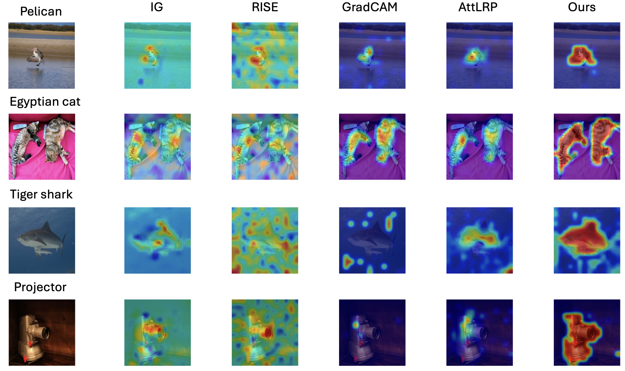
Figure 1: Qualitative examples for explaining the predictions in the image classification task. Our method yields more accurate visualizations compared to other baselines.

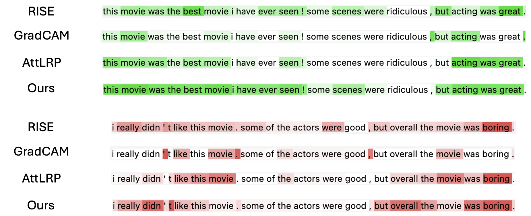
Figure 2: Qualitative examples for explaining the predictions in the sentiment classification task. Green indicates positive sentiment, red indicates negative.

	Random	IG	RISE	GradCAM	AttLRP	Ours
Positive AUC	0.6216	0.3837	0.3783	0.4608	0.2557	0.2659
Negative AUC	0.6229	0.8078	0.8668	0.6354	0.7996	0.8005
Pixel Acc	0.5064	0.5643	0.5225	0.6786	0.8162	0.8218
mAP	0.5050	0.6135	0.5448	0.7311	0.8590	0.9033
mIoU	0.3235	0.3714	0.3052	0.4458	0.6517	0.6679

Table 1: Quantitative evaluation results of different explanation methods for the image classification task. Note that for Positive AUC, the smaller the better, while for all other metrics, the larger the better. Our method performs consistently across all metrics.

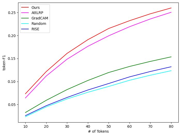
Figure 3: Quantitative evaluation results for the text classification task. The x-axis represents the number of text tokens inserted starting from the most important token, and the y-axis is the F1 score given that amount of tokens.

4.3 Results

Figure 1 and Figure 2 demonstrate the qualitative illustration of different explanation methods on both the image classification task and the sentiment classification task. We can observe that our approach can achieve comparable visualization quality to the model-specific methods AttLRP and GradCAM, and has much better visualization quality than model-agnostic methods IG and RISE.

The quantitative evaluation results for both task are reported in Table 1 and Figure 3. Our proposed method performs consistently over all evaluation metrics; the next best is AttLRP, a method specifically designed for transformers.

In Table 2, we describe the computational resources required for explaining 1000 images for image classification task, which substantiates our claim that our framework can achieve fast inference speed with low memory cost. Specifically, our method uses the same memory and is over 16$\times$ faster than AttLRP.

	IG	RISE	GradCAM	AttLRP	Ours
Inference Time	1090s	2120s	14.9s	106.8s	6.3s
Memory Usage	28.9GB	15.9GB	1.9GB	2GB	2GB

Table 2: Experiments on the inference cost for explaining 1000 image predictions of a pretrained ViT model. All experiments are conducted on the same machine with 8 CPU cores and 1 Nvidia A100 GPU.

limitations:

A limitation of our framework is its reliance on a training procedure, which may pose challenges when data privacy or prior data acquisition is a concern.

5 Conclusion

In this study, we addressed the persistent challenge in the field of explainable artificial intelligence (XAI) of balancing general applicability with inference speed. We identified that while model-agnostic methods are broadly applicable, they suffer from slow inference times, and model-specific methods, though efficient, are restricted to particular model architectures. To overcome these limitations, we proposed a novel framework that bridges the gap between these two approaches by requiring no assumptions about the prediction model’s structure and achieving high efficiency during inference, thereby ensuring real-time explanations.

Broader Impact

Our framework enhances transparency and trust in AI, crucial for applications in sectors like healthcare. It aids debugging and bias identification, supporting ethical AI use and regulatory compliance. However, risks include potential oversimplification of explanations and exposure of proprietary model details. Addressing these challenges is key to maximizing positive impact.

References

- [1] Yu Zhang, Peter Tiňo, Aleš Leonardis, and Ke Tang. A survey on neural network interpretability. IEEE Transactions on Emerging Topics in Computational Intelligence, 2021.
- [2] Amina Adadi and Mohammed Berrada. Peeking inside the black-box: A survey on explainable artificial intelligence (xai). IEEE Access, 6:52138–52160, 2018.
- [3] Samuel Henrique Silva and Peyman Najafirad. Opportunities and challenges in deep learning adversarial robustness: A survey. arXiv preprint arXiv:2007.00753, 2020.
- [4] Riccardo Miotto, Fei Wang, Shuang Wang, Xiaoqian Jiang, and Joel T Dudley. Deep learning for healthcare: review, opportunities and challenges. Briefings in bioinformatics, 19(6):1236–1246, 2018.
- [5] Ahmet Murat Ozbayoglu, Mehmet Ugur Gudelek, and Omer Berat Sezer. Deep learning for financial applications: A survey. Applied soft computing, 93:106384, 2020.
- [6] Sorin Grigorescu, Bogdan Trasnea, Tiberiu Cocias, and Gigel Macesanu. A survey of deep learning techniques for autonomous driving. Journal of field robotics, 37(3):362–386, 2020.
- [7] Shahin Atakishiyev, Mohammad Salameh, Hengshuai Yao, and Randy Goebel. Explainable artificial intelligence for autonomous driving: A comprehensive overview and field guide for future research directions. arXiv preprint arXiv:2112.11561, 2021.
- [8] Amitojdeep Singh, Sourya Sengupta, and Vasudevan Lakshminarayanan. Explainable deep learning models in medical image analysis. Journal of imaging, 6(6):52, 2020.
- [9] Ramprasaath R Selvaraju, Michael Cogswell, Abhishek Das, Ramakrishna Vedantam, Devi Parikh, and Dhruv Batra. Grad-cam: Visual explanations from deep networks via gradient-based localization. In Proceedings of the IEEE international conference on computer vision, pages 618–626, 2017.
- [10] Hila Chefer, Shir Gur, and Lior Wolf. Transformer interpretability beyond attention visualization. In Proceedings of the IEEE/CVF conference on computer vision and pattern recognition, pages 782–791, 2021.
- [11] Yao Qiang, Deng Pan, Chengyin Li, Xin Li, Rhongho Jang, and Dongxiao Zhu. Attcat: Explaining transformers via attentive class activation tokens. Advances in neural information processing systems, 35:5052–5064, 2022.
- [12] Marco Tulio Ribeiro, Sameer Singh, and Carlos Guestrin. " why should i trust you?" explaining the predictions of any classifier. In Proceedings of the 22nd ACM SIGKDD international conference on knowledge discovery and data mining, pages 1135–1144, 2016.
- [13] Scott M Lundberg and Su-In Lee. A unified approach to interpreting model predictions. In Advances in neural information processing systems, pages 4765–4774, 2017.
- [14] Vitali Petsiuk, Abir Das, and Kate Saenko. Rise: Randomized input sampling for explanation of black-box models. arXiv preprint arXiv:1806.07421, 2018.
- [15] Ruth C Fong and Andrea Vedaldi. Interpretable explanations of black boxes by meaningful perturbation. In Proceedings of the IEEE international conference on computer vision, pages 3429–3437, 2017.
- [16] Mukund Sundararajan, Ankur Taly, and Qiqi Yan. Axiomatic attribution for deep networks. In International Conference on Machine Learning, pages 3319–3328. PMLR, 2017.
- [17] Deng Pan, Xin Li, and Dongxiao Zhu. Explaining deep neural network models with adversarial gradient integration. In Thirtieth International Joint Conference on Artificial Intelligence (IJCAI), 2021.
- [18] Xin Li, Deng Pan, Chengyin Li, Yao Qiang, and Dongxiao Zhu. Negative flux aggregation to estimate feature attributions. arXiv preprint arXiv:2301.06989, 2023.
- [19] Avanti Shrikumar, Peyton Greenside, and Anshul Kundaje. Learning important features through propagating activation differences. In International conference on machine learning, pages 3145–3153. PMLR, 2017.
- [20] Scott M Lundberg, Gabriel G Erion, and Su-In Lee. Consistent individualized feature attribution for tree ensembles. arXiv preprint arXiv:1802.03888, 2018.
- [21] Volodymyr Mnih, Adria Puigdomenech Badia, Mehdi Mirza, Alex Graves, Timothy Lillicrap, Tim Harley, David Silver, and Koray Kavukcuoglu. Asynchronous methods for deep reinforcement learning. In International conference on machine learning, pages 1928–1937. PMLR, 2016.
- [22] John Schulman, Filip Wolski, Prafulla Dhariwal, Alec Radford, and Oleg Klimov. Proximal policy optimization algorithms. arXiv preprint arXiv:1707.06347, 2017.
- [23] Alexey Dosovitskiy, Lucas Beyer, Alexander Kolesnikov, Dirk Weissenborn, Xiaohua Zhai, Thomas Unterthiner, Mostafa Dehghani, Matthias Minderer, Georg Heigold, Sylvain Gelly, et al. An image is worth 16x16 words: Transformers for image recognition at scale. arXiv preprint arXiv:2010.11929, 2020.
- [24] Jia Deng, Wei Dong, Richard Socher, Li-Jia Li, Kai Li, and Li Fei-Fei. Imagenet: A large-scale hierarchical image database. In 2009 IEEE conference on computer vision and pattern recognition, pages 248–255. Ieee, 2009.
- [25] Jacob Devlin, Ming-Wei Chang, Kenton Lee, and Kristina Toutanova. Bert: Pre-training of deep bidirectional transformers for language understanding. arXiv preprint arXiv:1810.04805, 2018.
- [26] Richard Socher, Alex Perelygin, Jean Wu, Jason Chuang, Christopher D Manning, Andrew Y Ng, and Christopher Potts. Recursive deep models for semantic compositionality over a sentiment treebank. In Proceedings of the 2013 conference on empirical methods in natural language processing, pages 1631–1642, 2013.
- [27] Matthieu Guillaumin, Daniel Küttel, and Vittorio Ferrari. Imagenet auto-annotation with segmentation propagation. International Journal of Computer Vision, 110:328–348, 2014.
- [28] Jay DeYoung, Sarthak Jain, Nazneen Fatema Rajani, Eric Lehman, Caiming Xiong, Richard Socher, and Byron C Wallace. Eraser: A benchmark to evaluate rationalized nlp models. arXiv preprint arXiv:1911.03429, 2019.
- [29] Omar Zaidan and Jason Eisner. Modeling annotators: A generative approach to learning from annotator rationales. In Proceedings of the 2008 conference on Empirical methods in natural language processing, pages 31–40, 2008.