Lifelong Learning and Selective Forgetting via Contrastive Strategy

Abstract

Lifelong learning aims to train a model with good performance for new tasks while retaining the capacity of previous tasks. However, some practical scenarios require the system to forget undesirable knowledge due to privacy issues, which is called selective forgetting. The joint task of the two is dubbed Learning with Selective Forgetting (LSF). In this paper, we propose a new framework based on contrastive strategy for LSF. Specifically, for the preserved classes (tasks), we make features extracted from different samples within a same class compacted. And for the deleted classes, we make the features from different samples of a same class dispersed and irregular, i.e., the network does not have any regular response to samples from a specific deleted class as if the network has no training at all. Through maintaining or disturbing the feature distribution, the forgetting and memory of different classes can be or independent of each other. Experiments are conducted on four benchmark datasets, and our method acieves new state-of-the-art.

1 Introduction

Deep neural networks have achieved great success in many tasks based on powerful computing devices and large-scale training data. However, deep learning suffers from catastrophic forgetting, i.e., when the network learns new tasks, its performance for the previous tasks dramatically degrades. To solve this problem, lifelong learning (also called continual learning or incremental learning) has been put forward, where the network can continually learn new tasks without forgetting the previous tasks. Major approaches of lifelong learning can be categorized to regularization-based Kirkpatrick et al. (2017a), dynamic-architectures-based Wang et al. (2017) and replay-based Rebuffi et al. (2017). Meanwhile, as artificial intelligence enters every aspect of people’s lives, privacy protection and data leakage prevention receives more attention. The new challenges include privacy-preserving localization Speciale et al. (2019), learning from encrypted data Gilad-Bachrach et al. (2016), and so on. Lifelong learning cannot avoid this issue. Retaining the complete knowledge of all previous classes or tasks is a double-edged sword, which possibly leads to the risk of data leakage and invasion of privacy.

In order to solve the above mentioned problem, Learning with Selective Forgetting (LSF) is firstly proposed in Shibata et al. (2021), which aims to avoid catastrophic forgetting while selectively forget only specified sets of past classes. It designs a mnemonic code for each class to control which to forget and which to preserve, and only mnemonic codes belonging to preserved classes are used for the following training so as to enable the network to achieve selective forgetting. Despite being a pioneer, this method leaves much to be desired. Firstly, existing lifelong learning methods need to add an additional input (mnemonic codes) to achieve selective forgetting, but accurate generation of mnemonic codes is challenging for complex tasks like segmentation, which limits the usage. Secondly, it indirectly affects the feature extraction through the loss of the classification head. Intuitively, the direct operation of feature extraction is more effective and more universal (almost all deep learning has feature extraction part). Thirdly, it just simply ignores the loss of deleted classes but does no specific forgetting operation on them, leading to forgetting very slowly and inefficiently, and affecting the accuracy of the preserved classes.

Recently, contrastive learning shows significant advantages in lifelong learning Michieli and Zanuttigh (2021), and based on this, we make an improvement to make the lifelong learning system easily obtain the ability of selective forgetting. Specifically, for the preserved classes, we still follow the previous way of contrastive learning, i.e., making the aggregation of features within the class and the dispersion between the classes. For the deleted classes, we make the features of different samples (features of pixels or images) within a same class dispersed and irregular so as to make the network react as if it is untrained to achieve selective forgetting. Both forgetting and memory operate at the feature level (the embedding space), so they are very efficient and fast, and do not interfere with each other.

In conclusion, a more general strategy based on contrastive learning is proposed that perfectly incorporates lifelong learning and selective forgetting. Moreover, the proposed method directly operates on the feature extraction part to make the forgetting fast and universal, and thus can fundamentally avoid the possibility of information leakage. Experiments on three classification and a segmentation benchmark datasets show the significant superiority of the proposed approach.

2 Related Work

2.1 Lifelong Learning

Most of the current techniques of lifelong learning fall into three categories: regularization, dynamic- architectures, and replay-based.
Regularization-based: Regularization-based approaches are the most widely employed by far and mainly come in two flavours: penalty computing Kirkpatrick et al. (2017b) and knowledge distillation Li and Hoiem (2017); Cermelli et al. (2020). Penalty computing approaches prevent forgetting via limiting the change of important weights inside the models. Knowledge distillation relies on a teacher (old) model transferring knowledge to a student (new) model while the student model is still trained to learn new tasks.
Dynamic-architectures-based: Dynamic architectures grow new branches for new tasks, which can be explicit Wang et al. (2017), if new network branches are grown; or implicit Fernando et al. (2017), if some network weights are available for certain tasks only.
Replay-based: Replay-based models exploit storing or generating examples during the learning process of new tasks. Generative approaches Shin et al. (2017) rely on generative models, which are later used to generate artificial samples to preserve previous knowledge. Storage-based approaches Rebuffi et al. (2017) save a set of raw samples of past tasks for the following training.

Different from the pioneering work Shibata et al. (2021) using both the penalty and distillation, ours is only categorized to the knowledge distillation-based approach, which contains simple structure and is more suitable for complex tasks such as segmentation Cermelli et al. (2020); Cha et al. (2021).

2.2 Machine Unlearning

Recent legislation such as the General Data Protection Regulation (GDPR) enacts the “right to be forgotten”, which allows individuals to request the deletion of their data by the model owner to preserve their privacy. Moreover, any influence of the model about the target should also be removed. This process is referred to as machine unlearning (MU), which is first introduced by Cao and Yang (2015). General approaches are to train multiple small models on separated subsets of the training data to prevent retraining the whole knowledge Bourtoule et al. (2021) or to utilize vestiges of the learning process, i.e., the stored learned model parameters and the corresponding gradients Wu et al. (2020). Inspired by Differential Privacy (DP) Abadi et al. (2016), Eternal Sunshine of the Spotless Net Golatkar et al. (2020) introduced a scrubbing procedure that removes knowledge from the already trained weights of deep neural networks using the Fisher information matrix.

To the best of our knows, we firstly employ latent contrastive learning for MU, and the operation is directly on the feature extraction part.

2.3 Contrastive Learning

Contrastive learning has recently become a dominant component in self-supervised learning methods Jaiswal et al. (2021). It aims at embedding augmented versions of the same sample close to each other while trying to push away embeddings from different samples. In lifelong learning, SDR Michieli and Zanuttigh (2021) employs contrastive learning to cluster features according to their semantics while tearing apart those of different classes. We follow the framework of SDR and make an effective improvement to endow it the ability of selective forgetting without affecting the lifelong learning.

3 Problem Definition

$\left\{\mathcal{D}_{1},\cdots\mathcal{D}_{t},\cdots\mathcal{D}_{T}\right\}$ denotes a sequence of datasets, where $\mathcal{D}_{t}=\left\{\left(\mathbf{x}_{t}^{i},\mathbf{y}_{t}^{i}\right)_{i=1}^{n_{t}}\right\}$ is the dataset of the $t$-th task. $\mathcal{S}_{t}=\mathcal{C}_{1}\cup,\dots,\mathcal{C}_{t}$, which denotes classes that have been studied. We denote the input image space by $\mathcal{X}\in\mathbb{R}^{H\times W\times 3}$ with spatial dimensions $H$ and $W$, the set of classes (or categories) by $\mathcal{C}=\left\{c_{i}\right\}_{i=0}^{C}$, and the output space by $\mathcal{Y}\in\mathbb{R}^{H\times W}$ (i.e., the segmentation map), or $\mathcal{Y}\in\mathbb{R}^{1\times 1}$ for classification tasks. $\mathbf{x}_{t}^{i}\in\mathcal{X}$ is an input image, and $y_{t}^{i}\in\mathcal{Y}$ is the corresponding label.

In LSF problem, each of the learned classes is assigned to either preservation set or deletion set. Preservation Set $\mathcal{C}_{t}^{p}$ denotes a set of classes learned in the past and should be preserved at $t$-th task. Deletion Set $\overline{\mathcal{C}_{t}^{p}}$ denotes a set of classes should be forgotten until $t$-th task (the complement of $\mathcal{C}_{t}^{p}$). The objective of LSF is to learn a model $f_{\theta}:\mathcal{X}\rightarrow\mathcal{Y}$. For the classes from current learning set or preservation set, the network is expected to predict correctly. Otherwise, for the deletion set, the network is expected predicts wrongly. Our work goes a step further and makes deleted classes to be classified as background classes (if there is) to eliminate the impact on the accuracy of preserved classes. Note that the network does not change architecture like deleting or merging the segmentation head.

In lifelong learning, when new tasks start, samples of previously learned classes are not accessible Shibata et al. (2021); Cermelli et al. (2020), and both Shibata et al. (2021) and ours follow this rule. However, the information of the old classes can be obtained indirectly, such as mnemonic code in the classification task, or the old class data obtained through pseudo-labels in the segmentation task, which can be used to achieve forgetting or memory.

4 Proposed Method

4.1 Overview

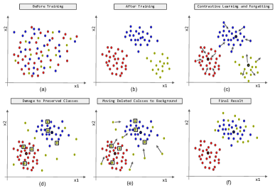
Figure 1: Feature distribution and operations on features. A color represents a class, and blue represents the background class. A dot means the feature of a sample (an image or a pixel). The features extracted from samples of the same class by untrained networks are scattered (shown in (a)), while the features from the trained networks are aggregated (shown in (b)). Inspired by this phenomenon, we calculate the global prototypes for each class (the bold dots in (c)), and then diverge features belonging to the same deleted class (green dots in (c)), but compact features of the same preserved class (blue and red dots in (c)). The above mentioned operations achieve selective forgetting but cause samples of deleted classes to be randomly categorized as any class, thus reducing the accuracy of preserved classes (the dots surrounded by black boxes in (d)). We move features of deleted classes close to background class (shown in (e)), so the deleted classes are resembled to the background class (shown in (f)) to avoid affecting others.

The Essence of Forgetting: If a network forgets a class, i.e., the network (including the feature extraction part and the classification part) does not contain any information about the class, thus no attack will lead to the leakage of information. In conclusion, forgetting means that the features extracted by the network for different samples of a same class are scattered and irregular in all feature spaces. Figure 1 is vital to understand our idea, intuitively showing our motivation and the proposed operations.

Following SDR Michieli and Zanuttigh (2021), we calculate one global (not limited to only one batch) prototype for each class, as shown in Section 4.2. Then, the prototypes are used to preserve and forget classes according to the mind of contrastive learning. Specifically, for the preserved classes, the network’s response is expected to be consistent and compacted for samples of a same class; for the deleted classes, our goal is to make the network respond randomly and irregularly as if the network has not been trained for this class at all. These procedures are introduced in Section 4.3. Meanwhile, for segmentation tasks, the features of deleted classes are moved close to background to avoid affecting the accuracy of other preserved classes, which is shown in Section 4.4.

Symbol definition: We use step $t$ as the example, since the operations at different steps are consistent, we omit the flag $t$ for simplicity. $\mathbf{y}^{\prime}_{n}=f_{\theta}\left(\mathbf{x}_{n}\right)$. $f_{\theta}\left(\mathbf{x}_{n}\right)[h,w,c]$ is the probability for class $c$ in pixel $(h,w)$, where $h=1,\dots,H,w=1,\dots,W$. And the output segmentation mask is computed as ${\mathbf{\tilde{y}}}_{n}=\arg\max_{c\in\mathcal{C}}f_{\theta}\left(\mathbf{x}_{n}\right)$. The background in ground truth ${\mathbf{y}_{n}}$ is replaced by the $\mathbf{\tilde{y}}_{n}$ of the previous step (step $t-$1), and the modified result is a comprehensive supervised information (pseudo label), called $\hat{\mathbf{y}}_{n}$. The rationale behind this operation is that the prediction of old model to old classes is reliable, and the background class could incorporates statistics of previous classes. Nowadays, for segmentation tasks, $f_{\theta}$ is typically an auto-encoder model made by an encoder $E$ and a decoder $D$ (i.e., $f_{\theta}=D\circ E$ ). We call $\mathbf{F}_{n}=E\left(\mathbf{x}_{n}\right)$ the feature map of $\mathbf{x}_{n}$, and $\mathbf{y}_{n}^{*}$ is the downsampled comprehensive pseudo label (i.e., $\hat{\mathbf{y}}_{n}$) matching the spatial dimensions of $\mathbf{F}_{n}$. For classification tasks, just change the pixel-level to image-level and pseudo label to mnemonic code to get the old class information, and the rest are the same.

4.2 Global Prototypes Calculation

Prototypes (i.e., class-centroids) are vectors that are representative of each class, and we follow SDR to calculate the global prototype rather than prototype limited only to one batch.

For the current batch $\mathcal{B}$ with $B$ images, the current (or in-batch) prototypes $\hat{\mathbf{p}}_{c}[t]$ at $t$-th step are computed as the average of the features of class $c$, and the specific form is shown as,

$$\hat{\mathbf{p}}_{c}[t]=\frac{1}{B}\sum_{\mathbf{x}_{n}\in\mathcal{B}}\frac{\sum_{\mathbf{f}_{i}\in\mathbf{F}_{n}}\mathbf{f}_{i}\mathbbm{1}\left[y_{i}^{*}=c\right]}{\mid\mathbbm{1}\left[\mathbf{y}_{n}^{*}=c]|\right.},$$ (1)

where $\mathbf{f}_{i}\in\mathbf{F}_{n}$ is a generic feature vector and $y_{i}^{*}$ is the corresponding pixel label in $\mathbf{y}_{n}^{*}$. $\mathbbm{1}\left[\mathbf{y}_{n}^{*}=c\right]$ indicates the pixels in $\mathbf{y}_{n}^{*}$ associated to $c$, and when the label corresponding to the feature is class $c$, the value is 1; otherwise, the value is 0. $|\cdot|$ denotes cardinality.

At training step $t$ with batch $\mathcal{B}$ of $B$ images, the global prototypes $\mathbf{p}_{c}[t]$ are updated for a generic class $c$ as:

$$\mathbf{p}_{c}[t]=\frac{1}{t}\left((t-1)\mathbf{p}_{c}[t-1]+\hat{\mathbf{p}}_{c}[t]\right),$$ (2)

which is initialized to $\mathbf{p}_{c}[0]=\mathbf{0}$ $\forall c$. For classification tasks, an image has only one output, and the calculation method is the same.

4.3 Lifelong Learning and Selective Forgetting

Lifelong Learning: Contrastive learning is to structure the latent space to make features of the same class clustered near their prototype, which also helps in lifelong learning to mitigate forgetting and to facilitate the addition of novel classes. Formally, for the features within the same preserved classes, we define $\mathcal{L}_{in}^{p}$ to maintain the aggregation of in-class features, as follows:

$$\mathcal{L}_{in}^{p}=\frac{1}{N_{c}^{p}}\sum\limits_{c_{j}\in(\mathcal{C}^{p}_{t}\cup\mathcal{C}_{t})\atop c_{j}\in\mathbf{y}_{n}^{*}}\sum\limits_{\mathbf{f}_{i}\in\mathbf{F}_{n}}\|\left(\mathbf{f}_{i}-\mathbf{p}_{c_{j}}\right)\mathbbm{1}\left[y_{i}^{*}=c_{j}]\|_{F}\right.,$$ (3)

where $N_{c}^{p}=\left|c_{j}\in\mathbf{y}_{n}^{*}\cap c_{j}\in(\mathcal{C}^{p}_{t}\cup\mathcal{C}_{t})\right|$, denoting the number of classes to be learned and preserved in $\mathbf{F}_{n}$. We use the Frobenius norm $\|\cdot\|_{F}$ as metric distance. $\mathcal{L}_{in}^{p}$ actually measures how close features are from their respective centroids, and its objective is to make feature vectors from the same preserved class are tightened around class feature centroids. The effect of $\mathcal{L}_{in}^{p}$ corresponds to the arrows surrounding red and blue dots in Figure 1 (c). For classification tasks, $\mathbf{F}_{n}$ is both the feature extracted from images (the feature of the current learning classes) and the feature extracted from mnemonic codes (the feature of the already learned classes).

Selective Forgetting: On the contrary, if we want the network to forget a certain class, we can make the features within the class move away from the prototype at different distances and in all directions. This requirement can be nicely satisfied, as shown below:

$$\mathcal{L}_{in,\mathbf{F}_{n}}^{d}=\frac{1}{N_{c}^{d}}\sum\limits_{c_{j}\in\overline{\mathcal{C}^{p}_{t}}\atop c_{j}\in\mathbf{y}_{n}^{*}}\sum\limits_{\mathbf{f}_{i}\in\mathbf{F}_{n}}\frac{1}{\|\left(\mathbf{f}_{i}-\mathbf{p}_{c_{j}}\right)\mathbbm{1}\left[y_{i}^{*}=c_{j}\right]\|_{F}},$$ (4)

where $N_{c}^{d}=\left|c_{j}\in\mathbf{y}_{n}^{*}\cap c_{j}\in\overline{\mathcal{C}^{p}_{t}}\right|$. Furthermore, the distribution of same feature are different at diverse spaces. Based on this, we not only perform in-class dispersion in the last layer of feature extraction, but also add two $3\times 3$ convolutions after the output to change its feature dimensions to the $\frac{1}{2}$ and $\frac{1}{4}$ of original size (spatial size keeps same), and then carries out feature dispersion operation in these three feature spaces. The two convolution can be thought of as a dimensional reduction operation, such that the feature is divergent from various embedding spaces. Therefore, $\mathcal{L}_{in}^{d}$ are computed as,

$$\mathcal{L}_{in}^{d}=\mathcal{L}_{in,\mathbf{F}_{n}}^{d}+\mathcal{L}_{in,\mathbf{F}_{n}^{*}}^{d}+\mathcal{L}_{in,\mathbf{F}_{n}^{**}}^{d},$$ (5)

where $\mathbf{F}_{n}^{*}$ and $\mathbf{F}_{n}^{**}$ is the output of $\mathbf{F}_{n}$ after one and two $1\times 1$ convolutions. Note that the two additional features are only used to calculate $\mathcal{L}_{in}^{d}$ and do not enter the decoder part of the segmentation or the classifier of the classification networks.

4.4 Making Deleted Classes Fall into Background

Contrast learning can not only make the features within a same class close together, but also make different classes subject to a repulsive force, thus moving them apart. We utilize $\mathcal{L}_{ex}^{p}$ to measure how far prototypes corresponding to different semantic classes are, i.e.,

$$\mathcal{L}_{ex}^{p}=\frac{1}{N_{c}^{p}}\sum_{\begin{subarray}{c}c_{j}\in(\mathcal{C}_{t}^{p}\cup\mathcal{C}_{t})\\ c_{j}\in\mathbf{y}_{n}^{*}\end{subarray}}\sum_{\begin{subarray}{c}c_{k}\in\mathbf{y}_{n}^{*}\\ c_{k}\neq c_{j}\end{subarray}}\frac{1}{\|\hat{\mathbf{p}}_{c_{j}}-\hat{\mathbf{p}}_{c_{k}}\|_{F}}$$ (6)

There are background in the segmentation task, i.e., others except the foreground classes are labeled as background. A reasonable and feasible approach that prevent affecting the accuracy of the preserved classes is to move them close to the background to avoid false positives, as shown in Figure 1 (e). The loss function to achieve this goal is shown as below,

$$\mathcal{L}_{ex}^{d}=\frac{1}{N_{c}^{d}}\sum\limits_{\mathbf{f}_{i}\in\mathbf{F}_{n}}\|\left(\mathbf{f}_{i}-\mathbf{p}_{b}\right)\mathbbm{1}[y_{i}^{*}\in\overline{\mathcal{C}_{t}^{p}}]\|_{F},$$ (7)

where $\mathbf{p}_{b}$ is the prototype of background, and $N_{c}^{d}$ denotes the number of deleted classes in $\mathbf{F}_{n}$.

4.5 Total Loss

Consistent with SDR, to keep the effectiveness of global prototypes, we introduce $\mathcal{L}_{pc}$ to ensure the validity of the global prototype. More formally,

$$\mathcal{L}_{pc}=\frac{1}{\left|\mathcal{S}_{t-1}\right|}\left\|\mathbf{p}_{c}-\hat{\mathbf{p}}_{c}\right\|_{F}\quad c\in\mathcal{S}_{t-1}$$ (8)

We modify the distillation loss from the whole previous learned classes $\mathcal{S}_{t}$ to only preserved classes $\mathcal{C}^{p}_{t}$, i.e.,

$$\mathcal{L}_{dis}=-\frac{1}{WH}\sum_{w,h}\sum_{c\in\mathcal{C}^{p}_{t}}{y}^{\prime\prime}(w,h,c)\log{y}^{\prime}(w,h,c),$$ (9)

where ${y}^{\prime\prime}$ is the output of the previous step (step $t-$1) model to keep the memory of already learned classes.

Therefore, the training objective is summed as:

$$\mathcal{L}_{tot}=\mathcal{L}_{ce}+\mathcal{L}_{dis}+\mathcal{L}_{pc}+\lambda_{p}\cdot(\mathcal{L}_{in}^{p}+\mathcal{L}_{ex}^{p})+\lambda_{d}\cdot(\mathcal{L}_{in}^{d}+\mathcal{L}_{ex}^{d}),$$ (10)

where the weights balance the multiple losses. The weights are the same as SDR, except $\lambda_{p}$ and $\lambda_{d}$. Unless specified, $\lambda_{p}$=$\lambda_{d}$=0.001. And the results with different ratios of $\lambda_{p}$ and $\lambda_{d}$ have been shown in Section Sensitivity Analysis. $\mathcal{L}_{ce}$ is the cross-entropy loss to learn new classes. For classification tasks, there is no $\mathcal{L}_{ex}^{d}$ loss.

5 Experiments

5.1 Settings

Dataset: For classification tasks, we use three widely used benchmark datasets for lifelong learning, i.e., CIFAR-100, CUB200-2011 Wah et al. (2011), and Stanford Cars Krause et al. (2013). CUB200-2011 has 200 classes with 5,994 training images and 5,794 test images. CIFAR-100 contains 50,000 training images and 10,000 test images overall. Stanford Cars comprises 196 cars of 8,144 images for training and 8,041 for testing. Segmentation experiments are conducted on VOC (Pascal-VOC2012) Everingham and Winn (2011). The VOC contains 10,582 images in the training set and 1,449 in the validation set (that we use for testing, as done by all competing works because the test set not publicly available). Each pixel of each image is assigned to one semantic label chosen among 21 different classes (20 plus the background).

Cross-validation is used, i.e., 20% of the training set is as the real validation set. In line with Shibata et al. (2021), the first 30% of classes for each task belongs to the deletion set, while the other classes belong to the preservation set. If the number of the first 30% classes is not an integer, we use method of rounding up. We use the usually used overlapped setup for dataset division. In the first initial phase we select the subset of training images having only $\mathcal{C}_{0}$-labeled pixels. Then, the training set at each incremental step contains the images with labeled pixels from $\mathcal{C}_{t}$, i.e., $\mathcal{D}_{t}=\mathcal{X}\times\mathcal{Y}_{\mathcal{C}_{t}\cup\{b\}}$. Similar to the initial step, labels are limited to semantic classes in $\mathcal{C}_{t}$, while remaining pixels are assigned to $b$ (background).

Implementation details: For the classification task, as in MC Shibata et al. (2021), we used ResNet-18 He et al. (2016) as the model. The final layer was changed to the multi-head architecture as in MC. The network is trained for 200 epochs for each task. Minibatch sizes are 128 in CIFAR-100, and 32 for CUB-200-2011 and Stanford Cars. The weight decay was $5.0\times 10^{-4}$ and SGD is for optimization. A standard data augmentation strategy is employed: random crop, horizontal flip, and rotation. For segmentation task, we use the standard Deeplab-v3+ Chen et al. (2018) architecture with ResNet-101 He et al. (2016) as backbone with output stride of 16. SGD is used as optimiazation and with the same learning rate policy, momentum and weight decay as SDR. The first learning step involves an initial learning rate of $10^{-2}$, which is decreased to $10^{-3}$ for the following steps. The learning rate is decreased with a polynomial decay rule with power $0.9$. In each learning step we train the models with a batch size of 20 for 30 epochs. The images are croped to $512\times 512$ during both training and validation and the same data augmentation is applied, i.e., random scaling the input images using a factor from $0.5$ to $2.0$ and random left-right flipping.

Since the segmentation task can demonstrate the effectiveness of all our work, we conduct ablation experiments on the segmentation task. The backbones are all been initialized using a pre-trained model on ImageNet Deng et al. (2009). For the segmentation task, our project is based on Michieli and Zanuttigh (2021), and for the classification task, the project is based on Shibata et al. (2021), i.e., we can indirectly obtain the information of the forgotten classes through mnemonic code or pseudo-labels in the background. We use Pytorch to develop and train all the models on two NVIDIA 3090 GPUs. The new model is initialized with the parameters of the previous step model.

Introduction of comparison methods: We compare our proposed method with the popular and state-of-the-art distillation-based lifelong learning methods. Further more, we also compare the modified version of them specifically for the LSF task. To sum up, the specific methods compared are as follows:
- FT: Fine-tuning, trained using only the classification loss, which can be regarded as the upper bound of forgetting.
- EWC Kirkpatrick et al. (2017b), MAS Aljundi et al. (2018), LwF Li and Hoiem (2017), MiB Cermelli et al. (2020), SSUL Cha et al. (2021), SDR Michieli and Zanuttigh (2021), and MC Shibata et al. (2021).
- LwF^∗, EWC^∗, MiB^∗, SDR^∗, and SSUL^∗: Modified version of LwF,EWC, MiB and SDR, i.e., the distillation losses or restricted parameters are changed from the calculation of all classes to only the preserved classes.
- LE^∗: LwF^∗+EWC^∗.
- LM^∗: LwF^∗+MAS.
- MC_E: MC+LwF^∗+EWC^∗.
- MC_M: MC+LwF^∗+MAS.

Evaluation metric: We follow the evaluation metric $S$ of Shibata et al. (2021), which called Learning with Selective Forgetting Measure (LSFM). LSFM is calculated as the harmonic mean of the two standard evaluation measures for lifelong learning Chaudhry et al. (2018): the average accuracy $A_{t}$ for the preserved classes and the forgetting measure $F_{t}$ for the deleted classes, i.e.,

$$S_{t}=\frac{2\cdot A_{t}\cdot F_{t}}{A_{t}+F_{t}}.$$ (11)

The average accuracy $A_{t}$ is evaluated after the model has been trained until the $t$-th task. The specific definition is given by $A_{t}=\frac{1}{t}\sum_{p=1}^{t}a_{t,p}$, where $a_{t,p}$ is the accuracy for the $p$-th task after the training for the $t$-th task is completed. $A_{t}$ is evaluated only for the preserved classes. Similarly, the forgetting measure $F_{t}$ is computed for the deleted classes after completing the $t$-th task. This measure is given by $F_{t}=\frac{1}{t}\sum_{p=1}^{t}f_{t}^{p}$, where $f_{t}^{p}=\max_{l\in 1\cdots t}a_{l,p}-a_{t,p}$, which represents the largest gap (decrease) from the past to the current accuracy for the $p$-th task. This is evaluated only for the deleted classes. The ranges of $A_{t}$ and $F_{t}$ are both $[0,1]$. We also report the averages of $S_{t},A_{t}$ and $F_{t}$ after the last task has been completed, which are denoted by $S,A$, and $F$.

5.2 Results

	CIFAR-100		CUB-200-2011		Stanford Cars
	$\#$ Task:5, $\#$ Class:20		$\#$ Task:5, $\#$ Class:40		$\#$ Task:4, $\#$ Class:49
	$S\uparrow$	($A\uparrow$,$F\uparrow$)	$S\uparrow$	($A\uparrow$,$F\uparrow$)	$S\uparrow$	($A\uparrow$,$F\uparrow$)
FT	51.8	(39.7, 74.6)	42.2	(31.8, 62.9)	48.1	(41.1, 58.1)
EWC	48.6	(36.5, 72.4)	41.4	(33.0, 55.5)	48.7	(47.7, 49.8)
$EWC^{*}$	49.6	(36.6, 77.1)	42.1	(33.4, 56.9)	50.7	(46.2, 56.2)
MAS	47.5	(34.9, 74.2)	45.1	(34.9, 63.7)	48.8	(44.7, 53.8)
LwF	17.2	(79.1, 9.7)	15.2	(69.0, 8.5)	9.9	(88.1, 5.3)
$LwF^{*}$	68.2	(81.3, 58.8)	44.5	(68.3, 33.1)	53.7	(88.2, 38.6)
$LE^{*}$	67.6	(81.2, 58.0)	43.4	(69.3, 31.6)	52.8	(88.7, 37.6)
$LM^{*}$	66.4	(81.8, 55.8)	47.5	(69.7, 36.0)	50.6	(89.0, 35.3)
$MC_{M}$	73.2	(72.6, 73.8)	58.0	(63.1, 53.6)	72.2	(84.6, 63.0)
$MC_{E}$	79.6	(75.3, 84.4)	61.4	(66.0, 57.4)	73.7	(86.0, 64.5)
Ours	81.7	(78.2, 85.6)	64.0	(67.4, 61.0)	75.9	(87.2, 67.1)

Table 1: The results (%) on classification tasks.

Results on classification tasks: The results of various methods on classification tasks are shown in Table 1. ‘Task:5, Class:20’ denotes that there are 5 tasks (steps) and 20 classes are learned per task. It can be seen that LwF shows good performance on the memory for the preserved classes, but it performs poorly for the deleted classes. Although the modified version achieves some improvements, it is still not ideal. EWC, MAS, and their modified versions, due to the own limitations, have a poor memory for preserved classes; on the contrary, they have certain advantages in the performance of the deleted classes. This advantage is not of its advantage over unlearning, but because they forget almost all old classes. LE^∗ and LM^∗, as the combination of LwF^∗ and parameter update constraint-based methods, greatly make up for the shortcomings of LwF^∗ in forgetting ability and achieve very significant progress. As a network specially set up for LSF tasks, MC_E and MC_D make great progress compared to previous methods. Our method organizes the feature (embedding) space so that the classes are dispersed, reducing the coupling between different classes. In addition, we directly disperse the feature distribution of the deleted classes to make the forgetting more complete. Therefore, we have achieved the best results in the comprehensive performance of forgetting and memory.

	19-1 (two tasks)		15-5 (two tasks)		15-1 (six tasks)
	$S\uparrow$	($A\uparrow$,$F\uparrow$)	$S\uparrow$	($A\uparrow$,$F\uparrow$)	$S\uparrow$	($A\uparrow$,$F\uparrow$)
FT	27.2	(16.2, 85.6)	44.4	(29.6, 88.8)	16.4	(9.0, 89.9)
MiB	26.7	(82.8, 15.9)	8.7	(84.2, 4.6)	49.2	(40.3, 63.1)
MiB∗	26.3	(82.8, 15.6)	17.4	(83.7, 9.7)	52.5	(40.2, 75.7)
SSUL	20.2	(88.4, 11.4)	19.0	(86.2, 10.7)	47.5	(56.9, 40.7)
SSUL∗	21.7	(88.2, 12.4)	28.7	(81.6, 17.4)	48.1	(53.5, 43.7)
SDR	26.9	(79.6, 16.2)	22.5	(77.2, 13.2)	32.7	(20.0, 89.0)
SDR∗	34.8	(69.4, 23.2)	31.7	(75.4, 20.1)	31.9	(19.4, 89.2)
MCE	51.0	(49.2, 53.1)	49.0	(40.1, 63.0)	24.7	(14.4, 86.9)
LwF	47.0	(61.0, 38.3)	35.2	(66.6, 23.9)	24.2	(15.1, 61.0)
LwF∗	55.9	(58.9, 53.2)	63.7	(66.7, 61.0)	26.6	(15.6, 89.4)
Ours	70.0	(76.7, 50.6)	72.9	(67.1, 80.0)	56.3	(41.2, 88.7)

Table 2: The results (%) on segmentation tasks.

Results on segmentation tasks: Results on segmentation tasks Shan et al. (2021c, b); Shan and Wang (2021); Shan et al. (2021a, 2022); Shan and Wang (2022); Shan et al. (2023b, c, a); Wu et al. (2023); Zhao et al. (2023a, b, c, 2024) are shown in Table 2. In line with incremental segmentation tasks, we set three learning rules, i.e., 19-1 (delete fist six classes), 15-5 (delete fist five classes), and 15-1 (delete fist five classes). 15-1 is incremental learning one class in five steps, and the other two are similar. FT achieves the best forgetting performance, but it forgets all the previous learned classes, resulting in low accuracy of preserved classes. Compared with FT, LwF makes great progress in memory but loses much of forgetting capacity. The forgetting performance of LwF^∗ is significantly improved, and the memory capacity is not significantly decreased or even improved. MiB and MiB^∗ have strong memory capacity, but their forgetting capacities are poor in all three learning settings. SDR, SDR^∗, SSUL, and SSUL^∗ are better than LwF in memory capacity, and better than MiB in forgetting capacity, so they can be regarded as a compromise version. Although MC has a slight advantage in forgetting capacity, it has a great disadvantage in memory capacity, which because it adds mnemonic codes as extra information to the input during training, resulting in the inconsistent feature distribution between training and testing. Our method is the best in terms of overall performance, and the superiority is significant, which demonstrates the advantages of contrastive learning for LSF tasks on segmentation tasks.

	delete 5 classes		delete 1 class		delete 10 classes
	$S\uparrow$	($A\uparrow$,$F\uparrow$)	$S\uparrow$	($A\uparrow$,$F\uparrow$)	$S\uparrow$	($A\uparrow$,$F\uparrow$)
MiB∗	17.4	(83.7, 9.7)	40.0	(84.0, 23.7)	13.8	(85.3, 7.5)
SSUL∗	28.7	(81.6, 17.4)	46.2	(82.4, 32.1)	27.2	(75.2, 16.6)
SDR∗	31.7	(75.4, 20.1)	65.1	(71.6, 59.7)	31.1	(78.6, 19.4)
LwF∗	65.5	(70.7, 61.0)	74.7	(67.5, 83.6)	58.5	(80.8, 45.9)
Ours	72.9	(67.1,80.0)	80.8	(74.2,88.7)	66.4	(81.6,56.0)

Table 3: The results (%) with varying deleted classes on setting of 15-5, and deleted classes are at front (sorted by class labels).

Results with varying deleted classes: To give a more comprehensive picture to the performance of each method, we delete a different number of classes, and the results are shown in Table 3. Due to the inherent drawbacks of MC for segmentation, we do not compare it here. When forgetting fewer classes like forgetting only one class, all methods perform well, indicating that forgetting a class is less difficult. When forgetting 10 classes, the forgetting performance of each method decreases significantly. In all cases, our method shows the best performance.

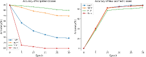
Figure 2: The accuracy of deleted classes and new learned classes on different epochs with the setting of 15-5.

Per-epoch results: Figure 2 shows the results during training. As can be seen, all methods perform similarly to learn new classes (as shown on the right graph), but differ widely to forget classes. Other methods (including LwF^∗ MiB^∗, and SDR^∗) forget the deleted classes only through not calculating the loss of deleted classes, so the forgetting speed is very slow. These approaches are more accurately described as not learning rather than forgetting the deleted classes. While our method makes targeted forgetting operation and directly act at the feature extraction part, so only 5 epochs are needed to reduce the accuracy of the deleted classes by 74.1 (89.3 to 15.2). In conclusion, the way we propose to break up the features within the same deleted classes makes forgetting incredibly efficient and fast.

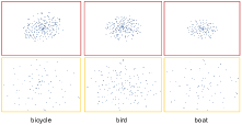
Figure 3: t-SNE plots of the features obtained from the last layer of the backbone before and after forgetting. Red boxes represents before forgetting and yellow is after, and the both are on the same scale. Each point represents the feature of a pixel (after downsampling), and the whole graph is the visualization result of the features in a batch (batchsize=20). Bicycle, bird and boat are belonged to the deleted classes.

Feature visualization: Figure 3 shows the feature distribution before and after forgetting. Since the classes are numerous and jumbled together, we only show the features of the deleted classes and show them separately to demonstrate the changes more clearly. It can be seen that the features of the same class become divergent and irregular from the previous compacted situation after the forgetting operation.

5.3 Ablation Study

$\mathcal{L}_{pc}$	$\mathcal{L}_{in}^{p}$	$\mathcal{L}_{ex}^{p}$	$\mathcal{L}_{in}^{d}$	$\mathcal{L}_{ex}^{d}$	$S\uparrow$	($A\uparrow$, $F\uparrow$)
$\checkmark$					63.9	(67.1, 61.0)
$\checkmark$	$\checkmark$				60.4	(68.2, 54.2)
$\checkmark$	$\checkmark$	$\checkmark$			61.0	(68.4, 55.1)
$\checkmark$			$\checkmark$		59.6	(47.4, 80.1)
$\checkmark$			$\checkmark$	$\checkmark$	63.5	(52.2, 81.2)
$\checkmark$	$\checkmark$	$\checkmark$	$\checkmark$		71.0	(64.3, 79.4)
$\checkmark$	$\checkmark$	$\checkmark$		$\checkmark$	61.2	(65.6, 57.4)
$\checkmark$	$\checkmark$	$\checkmark$	$\checkmark$	$\checkmark$	72.9	(67.1, 80.0)

Table 4: The results (%) with varying deleted classes on 15-5.

The effectiveness of different losses: The results of the respective effectiveness of losses are shown in Table 4. Among them, $\mathcal{L}_{pc}$ is to make the global and local prototypes consistent, and it is also the basis of the following series of operations. $\mathcal{L}_{in}^{p}$ and $\mathcal{L}_{ex}^{p}$ are used to retain feature compaction of preserved classes to keep the memory. It can be seen that after adding these two losses, the accuracy of preserved classes has been partially improved, but it also leads to incomplete forgetting of deleted classes. This phenomenon may be because $\mathcal{L}_{in}^{p}$ and $\mathcal{L}_{ex}^{p}$ increase the compaction within the class, and there is no disperse operation so that the network cannot forget the deleted classes. $\mathcal{L}_{in}^{d}$ is the key to ensure forgetting, which breaks up the feature distribution of the deleted classes to achieve forgetting. It can be seen that when $\mathcal{L}_{in}^{d}$ is added, the forgetting performance increases significantly. Without $\mathcal{L}_{in}^{p}$ and $\mathcal{L}_{ex}^{p}$, $\mathcal{L}_{in}^{d}$ also causes performance degradation for preserved classes. However, when $\mathcal{L}_{in}^{p}$, $\mathcal{L}_{ex}^{p}$ and $\mathcal{L}_{in}^{d}$ are all present, both the memory of preserved classes and the forgetting of deleted classes can be guaranteed. LSF can be achieved due these three losses make the feature distribution of the preserved classes stable while destroying the feature distribution of the deleted classes. After adding $\mathcal{L}_{ex}^{d}$, the results of deleted classes will not affect the performance of the preserved classes, avoiding false positives and thereby improving the performance. In a nutshell, all losses play roles and are indispensable.

$\mathbf{F}_{n}$	$\mathbf{F}_{n}^{*}$	$\mathbf{F}_{n}^{**}$	19-1	15-5	15-1
			$S\uparrow$	$S\uparrow$	$S\uparrow$
✓			66.7	69.4	55.7
✓	✓		69.1	72.2	56.1
✓	✓	✓	70.0	72.9	56.3

Table 5: The results (%) with divergence at different feature spaces.

Effectiveness of divergence of different feature spaces: In order to completely break up the feature distribution of the deleted classes, in addition to performing contrastive forgetting on the features extracted and used for the final classification, we also add two convolutions to perform the dispersion in a higher-dimensional embedding space. The results of contrastive forgetting in different embedding spaces are shown in Table 5. Adding $\mathbf{F}_{n}^{*}$ achieves an effect in all three different learning settings. However, after adding $\mathbf{F}_{n}^{**}$, the effect is not obvious and decreases in turn, which may be that the features of deleted classes have diverged enough in the embedding space to achieve forgetting. In a nutshell, the dispersion in the three embedding spaces all can bring improvements.

5.4 Sensitivity Analysis

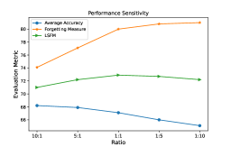
Figure 4: Sensitivity analysis. The abscissa represents the ratio of $\lambda_{p}$ to $\lambda_{d}$.

Memory of preserved classes and forgetting of deleted classes are two different goals, so it is of great significance to explore the weight of memory loss ($\mathcal{L}_{in}^{p}$ and $\mathcal{L}_{ex}^{p}$) and forgetting loss ($\mathcal{L}_{in}^{d}$ and $\mathcal{L}_{ex}^{d}$), i.e., $\lambda_{p}$ and $\lambda_{d}$. Consistent with SDR, the losses calculated from features are multiplied by 0.001, i.e., 1:1 is actually 0.001:0.001. The experimental results are shown in Figure 4. $\lambda_{p}$ corresponds to memory and $\lambda_{d}$ to forgetting. When $\lambda_{p}$ is large, the average accuracy of preserved classes is high, but the forgetting measure is relatively poor. When $\lambda_{p}$ gradually becomes smaller in the ratio ($\lambda_{d}$ becomes larger and gradually dominates), the forgetting measure becomes better, but the accuracy decreases. This phenomenon is consistent with the previous analysis. When $\lambda_{d}$ is small, the distribution of the deleted classes cannot be broken up, so complete forgetting cannot be achieved. When $\lambda_{p}$ is small, breaking up the forgotten category will affect the accuracy of the preserved classes and thus cause errors. Therefore, the best effect is obtained when the two are 1:1.

6 Conclusion

In this paper, an LSF method based on a contrastive strategy is proposed to perform direct forgetting by computing the dispersion loss for the deleted classes, which destroys the distribution of the deleted classes to quickly achieve selective forgetting without affecting the feature distribution of the preserved classes. The effectiveness of the proposed method is demonstrated in classification and segmentation tasks. Besides, the forgetting operation is performed in the feature extraction part, so it can be easily extended to other tasks (almost all deep learning-based models need to extract features). Our approach has implications for the continual and safe use of deep learning-based software in practical applications. In future works, how to better deal with the features of the deleted classes that have been dispersed to prevent false positives is a problem that needs to be solved. Similarly, exploring the learning ability and interpretability of neural networks from the aspect of feature distribution rather than the network structure is also a direction worth exploring.

References

- Abadi et al. [2016] Martin Abadi, Andy Chu, Ian Goodfellow, H Brendan McMahan, Ilya Mironov, Kunal Talwar, and Li Zhang. Deep learning with differential privacy. In Proceedings of the 2016 ACM SIGSAC conference on computer and communications security, pages 308–318, 2016.
- Aljundi et al. [2018] Rahaf Aljundi, Francesca Babiloni, Mohamed Elhoseiny, Marcus Rohrbach, and Tinne Tuytelaars. Memory aware synapses: Learning what (not) to forget. In Proceedings of the European Conference on Computer Vision (ECCV), pages 139–154, 2018.
- Bourtoule et al. [2021] Lucas Bourtoule, Varun Chandrasekaran, Christopher A Choquette-Choo, Hengrui Jia, Adelin Travers, Baiwu Zhang, David Lie, and Nicolas Papernot. Machine unlearning. In 2021 IEEE Symposium on Security and Privacy (SP), pages 141–159. IEEE, 2021.
- Cao and Yang [2015] Yinzhi Cao and Junfeng Yang. Towards making systems forget with machine unlearning. In 2015 IEEE Symposium on Security and Privacy, pages 463–480. IEEE, 2015.
- Cermelli et al. [2020] Fabio Cermelli, Massimiliano Mancini, Samuel Rota Bulo, Elisa Ricci, and Barbara Caputo. Modeling the background for incremental learning in semantic segmentation. In Proceedings of the IEEE/CVF Conference on Computer Vision and Pattern Recognition, pages 9233–9242, 2020.
- Cha et al. [2021] Sungmin Cha, YoungJoon Yoo, Taesup Moon, et al. Ssul: Semantic segmentation with unknown label for exemplar-based class-incremental learning. Advances in Neural Information Processing Systems, 34:10919–10930, 2021.
- Chaudhry et al. [2018] Arslan Chaudhry, Marc’Aurelio Ranzato, Marcus Rohrbach, and Mohamed Elhoseiny. Efficient lifelong learning with a-gem. arXiv preprint arXiv:1812.00420, 2018.
- Chen et al. [2018] Liang-Chieh Chen, Yukun Zhu, George Papandreou, Florian Schroff, and Hartwig Adam. Encoder-decoder with atrous separable convolution for semantic image segmentation. In Proceedings of the European conference on computer vision (ECCV), pages 801–818, 2018.
- Deng et al. [2009] Jia Deng, Wei Dong, Richard Socher, Li-Jia Li, Kai Li, and Li Fei-Fei. Imagenet: A large-scale hierarchical image database. In 2009 IEEE Conference on Computer Vision and Pattern Recognition, pages 248–255, 2009.
- Everingham and Winn [2011] Mark Everingham and John Winn. The pascal visual object classes challenge 2012 (voc2012) development kit. Pattern Analysis, Statistical Modelling and Computational Learning, Tech. Rep, 8:5, 2011.
- Fernando et al. [2017] Chrisantha Fernando, Dylan Banarse, Charles Blundell, Yori Zwols, David Ha, Andrei A Rusu, Alexander Pritzel, and Daan Wierstra. Pathnet: Evolution channels gradient descent in super neural networks. arXiv preprint arXiv:1701.08734, 2017.
- Gilad-Bachrach et al. [2016] Ran Gilad-Bachrach, Nathan Dowlin, Kim Laine, Kristin Lauter, Michael Naehrig, and John Wernsing. Cryptonets: Applying neural networks to encrypted data with high throughput and accuracy. In International conference on machine learning, pages 201–210. PMLR, 2016.
- Golatkar et al. [2020] Aditya Golatkar, Alessandro Achille, and Stefano Soatto. Eternal sunshine of the spotless net: Selective forgetting in deep networks. In Proceedings of the IEEE/CVF Conference on Computer Vision and Pattern Recognition, pages 9304–9312, 2020.
- He et al. [2016] Kaiming He, Xiangyu Zhang, Shaoqing Ren, and Jian Sun. Deep residual learning for image recognition. In Proceedings of the IEEE conference on computer vision and pattern recognition, pages 770–778, 2016.
- Jaiswal et al. [2021] Ashish Jaiswal, Ashwin Ramesh Babu, Mohammad Zaki Zadeh, Debapriya Banerjee, and Fillia Makedon. A survey on contrastive self-supervised learning. Technologies, 9(1):2, 2021.
- Kirkpatrick et al. [2017a] James Kirkpatrick, Razvan Pascanu, Neil Rabinowitz, Joel Veness, Guillaume Desjardins, Andrei A Rusu, Kieran Milan, John Quan, Tiago Ramalho, Agnieszka Grabska-Barwinska, et al. Overcoming catastrophic forgetting in neural networks. Proceedings of the national academy of sciences, 114(13):3521–3526, 2017.
- Kirkpatrick et al. [2017b] James Kirkpatrick, Razvan Pascanu, Neil Rabinowitz, Joel Veness, Guillaume Desjardins, Andrei A Rusu, Kieran Milan, John Quan, Tiago Ramalho, Agnieszka Grabska-Barwinska, et al. Overcoming catastrophic forgetting in neural networks. Proceedings of the national academy of sciences, 114(13):3521–3526, 2017.
- Krause et al. [2013] Jonathan Krause, Michael Stark, Jia Deng, and Li Fei-Fei. 3d object representations for fine-grained categorization. In Proceedings of the IEEE international conference on computer vision workshops, pages 554–561, 2013.
- Li and Hoiem [2017] Zhizhong Li and Derek Hoiem. Learning without forgetting. IEEE transactions on pattern analysis and machine intelligence, 40(12):2935–2947, 2017.
- Michieli and Zanuttigh [2021] Umberto Michieli and Pietro Zanuttigh. Continual semantic segmentation via repulsion-attraction of sparse and disentangled latent representations. In Proceedings of the IEEE/CVF Conference on Computer Vision and Pattern Recognition, pages 1114–1124, 2021.
- Rebuffi et al. [2017] Sylvestre-Alvise Rebuffi, Alexander Kolesnikov, Georg Sperl, and Christoph H Lampert. icarl: Incremental classifier and representation learning. In Proceedings of the IEEE conference on Computer Vision and Pattern Recognition, pages 2001–2010, 2017.
- Shan and Wang [2021] Lianlei Shan and Weiqiang Wang. Densenet-based land cover classification network with deep fusion. IEEE Geoscience and Remote Sensing Letters, 19:1–5, 2021.
- Shan and Wang [2022] Lianlei Shan and Weiqiang Wang. Mbnet: a multi-resolution branch network for semantic segmentation of ultra-high resolution images. In ICASSP 2022-2022 IEEE International Conference on Acoustics, Speech and Signal Processing (ICASSP), pages 2589–2593. IEEE, 2022.
- Shan et al. [2021a] Lianlei Shan, Minglong Li, Xiaobin Li, Yang Bai, Ke Lv, Bin Luo, Si-Bao Chen, and Weiqiang Wang. Uhrsnet: A semantic segmentation network specifically for ultra-high-resolution images. In 2020 25th International Conference on Pattern Recognition (ICPR), pages 1460–1466. IEEE, 2021.
- Shan et al. [2021b] Lianlei Shan, Xiaobin Li, and Weiqiang Wang. Decouple the high-frequency and low-frequency information of images for semantic segmentation. In ICASSP 2021-2021 IEEE International Conference on Acoustics, Speech and Signal Processing (ICASSP), pages 1805–1809. IEEE, 2021.
- Shan et al. [2021c] Lianlei Shan, Weiqiang Wang, Ke Lv, and Bin Luo. Class-incremental learning for semantic segmentation in aerial imagery via distillation in all aspects. IEEE Transactions on Geoscience and Remote Sensing, 60:1–12, 2021.
- Shan et al. [2022] Lianlei Shan, Weiqiang Wang, Ke Lv, and Bin Luo. Class-incremental semantic segmentation of aerial images via pixel-level feature generation and task-wise distillation. IEEE Transactions on Geoscience and Remote Sensing, 60:1–17, 2022.
- Shan et al. [2023a] Leo Shan, Wenzhang Zhou, and Grace Zhao. Incremental few shot semantic segmentation via class-agnostic mask proposal and language-driven classifier. In Proceedings of the 31st ACM International Conference on Multimedia, pages 8561–8570, 2023.
- Shan et al. [2023b] Lianlei Shan, Weiqiang Wang, Ke Lv, and Bin Luo. Boosting semantic segmentation of aerial images via decoupled and multi-level compaction and dispersion. IEEE Transactions on Geoscience and Remote Sensing, 2023.
- Shan et al. [2023c] Lianlei Shan, Guiqin Zhao, Jun Xie, Peirui Cheng, Xiaobin Li, and Zhepeng Wang. A data-related patch proposal for semantic segmentation of aerial images. IEEE Geoscience and Remote Sensing Letters, 20:1–5, 2023.
- Shibata et al. [2021] Takashi Shibata, Go Irie, Daiki Ikami, and Yu Mitsuzumi. Learning with selective forgetting. In International Joint Conference on Artificial Intelligence, 2021.
- Shin et al. [2017] Hanul Shin, Jung Kwon Lee, Jaehong Kim, and Jiwon Kim. Continual learning with deep generative replay. arXiv preprint arXiv:1705.08690, 2017.
- Speciale et al. [2019] Pablo Speciale, Johannes L Schonberger, Sing Bing Kang, Sudipta N Sinha, and Marc Pollefeys. Privacy preserving image-based localization. In Proceedings of the IEEE/CVF Conference on Computer Vision and Pattern Recognition, pages 5493–5503, 2019.
- Wah et al. [2011] Catherine Wah, Steve Branson, Peter Welinder, Pietro Perona, and Serge Belongie. The caltech-ucsd birds-200-2011 dataset. 2011.
- Wang et al. [2017] Yu-Xiong Wang, Deva Ramanan, and Martial Hebert. Growing a brain: Fine-tuning by increasing model capacity. In Proceedings of the IEEE Conference on Computer Vision and Pattern Recognition, pages 2471–2480, 2017.
- Wu et al. [2020] Yinjun Wu, Edgar Dobriban, and Susan Davidson. Deltagrad: Rapid retraining of machine learning models. In International Conference on Machine Learning, pages 10355–10366. PMLR, 2020.
- Wu et al. [2023] Weijia Wu, Yuzhong Zhao, Zhuang Li, Lianlei Shan, Hong Zhou, and Mike Zheng Shou. Continual learning for image segmentation with dynamic query. IEEE Transactions on Circuits and Systems for Video Technology, 2023.
- Zhao et al. [2023a] Yuzhong Zhao, Yuanqiang Cai, Weijia Wu, and Weiqiang Wang. Explore faster localization learning for scene text detection. In 2023 IEEE International Conference on Multimedia and Expo (ICME), pages 156–161. IEEE, 2023.
- Zhao et al. [2023b] Yuzhong Zhao, Weijia Wu, Zhuang Li, Jiahong Li, and Weiqiang Wang. Flowtext: Synthesizing realistic scene text video with optical flow estimation. In 2023 IEEE International Conference on Multimedia and Expo (ICME), pages 1517–1522. IEEE, 2023.
- Zhao et al. [2023c] Yuzhong Zhao, Qixiang Ye, Weijia Wu, Chunhua Shen, and Fang Wan. Generative prompt model for weakly supervised object localization. In Proceedings of the IEEE/CVF International Conference on Computer Vision, pages 6351–6361, 2023.
- Zhao et al. [2024] Yuzhong Zhao, Yue Liu, Zonghao Guo, Weijia Wu, Chen Gong, Fang Wan, and Qixiang Ye. Controlcap: Controllable region-level captioning, 2024.