When and How Does In-Distribution Label Help Out-of-Distribution Detection?

Abstract

Detecting data points deviating from the training distribution is pivotal for ensuring reliable machine learning. Extensive research has been dedicated to the challenge, spanning classical anomaly detection techniques to contemporary out-of-distribution (OOD) detection approaches. While OOD detection commonly relies on supervised learning from a labeled in-distribution (ID) dataset, anomaly detection may treat the entire ID data as a single class and disregard ID labels. This fundamental distinction raises a significant question that has yet to be rigorously explored: when and how does ID label help OOD detection? This paper bridges this gap by offering a formal understanding to theoretically delineate the impact of ID labels on OOD detection. We employ a graph-theoretic approach, rigorously analyzing the separability of ID data from OOD data in a closed-form manner. Key to our approach is the characterization of data representations through spectral decomposition on the graph. Leveraging these representations, we establish a provable error bound that compares the OOD detection performance with and without ID labels, unveiling conditions for achieving enhanced OOD detection. Lastly, we present empirical results on both simulated and real datasets, validating theoretical guarantees and reinforcing our insights. Code is publicly available at https://github.com/deeplearning-wisc/id_label.

1 Introduction

When deployed in the real world, machine learning models often encounter unfamiliar data points that fall outside the distribution of the observed data. This problem has been studied extensively, dating from the classical anomaly detection methods (Chandola et al., 2009; Ahmed & Courville, 2020; Han et al., 2022) to contemporary out-of-distribution (OOD) approaches (Liu et al., 2020b; Yang et al., 2021b; Fang et al., 2022).

While both anomaly detection and OOD detection share the goal of identifying test-time input that deviates from the training distribution, a crucial distinction lies in the usage of in-distribution (ID) labels in training time. Specifically, classical anomaly detection may disregard ID labels (Yang et al., 2021b), treating the entire ID dataset as a single class. In contrast, OOD detection commonly relies on supervised learning from a labeled ID dataset. It is reasonable to hypothesize that incorporating ID labels during training might influence the resulting feature representations, potentially leading to distinct capabilities in separating ID from OOD samples during test time. This raises a significant question that has yet to be rigorously explored in the field:

RQ: When and how does ID label help OOD detection?

Answering this question offers the fundamental key to understanding and bridging two highly related fields of anomaly detection and OOD detection. In pursuit of this objective, we provide a formal understanding to theoretically delineate the influence of ID labels on OOD detection. We base our analysis on a graph-theoretic approach by modeling the ID data via a graph, where the vertices are all the data points and edges encode the similarity among data. This analytical framework is well-suited for our investigation, as data points’ representation similarity can differ between the self-supervised and supervised learning setting, contingent upon the availability of ID labels. For instance, when ID labels are present, the supervisory signal facilitates connecting points belonging to the same class, resulting in each class manifesting as a distinct connected sub-graph. In both cases (with or without ID labels), the sub-structures can be revealed by performing spectral decomposition on the graph and can be expressed equivalently as a contrastive learning objective on neural net representations (expounded further in Section 3). Importantly, these learned feature representations allow us to rigorously analyze the separability of ID data from OOD data in a closed-form manner.

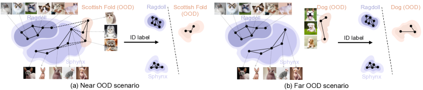
Figure 1: Intuitive example on the ID labels’ impact on OOD detection. (a) In the near OOD scenario where the OOD data connects densely with the ID data, without ID labels, the neural network produces indistinguishable embeddings for the ID (Ragdoll and Sphynx class) and OOD data (Scottish Fold class). By harnessing the power of the ID labeling information, the model learns more distinguishable embeddings that help ID vs. OOD separation. (b) In the far OOD scenario (Dog class), ID labels can be less beneficial because the representations learned in an unsupervised manner can already be separable between ID vs OOD.

Based on the analytical framework, we provide a formal error bound in Theorem 1, comparing the OOD detection performance with and without the inclusion of ID labels. This theorem reveals sufficient conditions for achieving improved OOD detection performance by leveraging ID labels. To establish the error bound, we first calculate the closed-form solution of the ID and OOD representations based on the graph factorization and then quantify the OOD detection performance by linear probing error. As a result, Theorem 1 demonstrates that the difference in the OOD detection performance with and without ID labels can be lower bounded by a function of the adjacency matrix of ID data as well as the OOD-ID connectivity. Furthermore, we offer intuitive interpretations in Theorem 2, and show that the ID labels are the most beneficial when either: (i) the OOD data is relatively close to the ID data, which is also known as the near OOD scenario; (ii) the ID data are connected sparsely without ID labels; and (iii) the semantic connection between each ID data to the labeled ID data from different ID classes is sufficiently large. To help readers understand the key insights of our theory, we provide a simple intuitive example in Figure 1, which demonstrates how adding ID labels in the near OOD scenario can lead to a greater benefit compared to the far OOD scenario.

Lastly, we provide empirical verifications to support our theory. In particular, we compare the OOD detection performance with and without ID labels using both simulated data and real-world datasets (Section 5). The result aligns with our theoretical guarantee, showcasing the benefits of the ID label information under proper conditions. For example, the OOD detection result can be improved by 12.3% (AUROC) in the near OOD scenario compared to 6.06% in the far OOD scenario on Cifar100, validating our theory.

Our main contributions are summarized as follows:

• We study an important but underexplored problem: when and how in-distribution labels can help OOD detection. Our exposition has fundamental value in understanding and bridging the two highly related fields of anomaly detection and OOD detection.

• We provide an analytical framework based on graph formulation to characterize the ID and OOD representations. Based on that, we analyze the error bound for ID vs. OOD separation with and without ID labels and investigate the necessary conditions for which the labeling information can bring the most benefits.

• We present empirical analysis on both simulated and real-world datasets to verify and support our theory. The observation in practice echoes and reinforces our theoretical insights.

2 Problem Setup

Let $\mathcal{X}$ be the input space, and $\mathcal{Y}=\{1,...,c\}$ be the label space for ID data. Given an unknown ID joint distribution $\mathbb{P}_{\mathcal{X}\mathcal{Y}}$ defined over $\mathcal{X}\times\mathcal{Y}$, the labeled ID data $\mathcal{S}_{\rm id}^{(l)}=\{(\mathbf{x}_{1},y_{1}),...,(\mathbf{x}_{N},y_{N})\}$ are drawn independently and identically from $\mathbb{P}_{\mathcal{X}\mathcal{Y}}$. Alternatively, the unlabeled ID data $\mathcal{S}_{\rm id}^{(u)}=\{\mathbf{x}_{1},...,\mathbf{x}_{N}\}$ is drawn from $\mathbb{P}_{\rm id}$, which is the marginal distribution of $\mathbb{P}_{\mathcal{X}\mathcal{Y}}$ on $\mathcal{X}$. Furthermore, we denote $\mathbb{P}_{l_{i}}$ the distribution of labeled data with label $i\in\mathcal{Y}$.

Definition 1 (Out-of-Distribution Detection w/ ID Labels).

Given labeled ID data $\mathcal{S}_{\rm id}^{(l)}$, the aim is to learn a predictor $\mathbf{g}:\mathcal{X}\rightarrow\mathcal{Y}\cup\{{\rm ood}\}$ such that for any test data $\mathbf{x}$: 1) if $\mathbf{x}$ is drawn from $\mathbb{P}_{\rm id}$, then the model classifies $\mathbf{x}$ into one of ID classes $\mathcal{Y}$, and 2) if $\mathbf{x}$ is drawn from another distribution $\mathbb{P}_{\rm ood}$ with unknown OOD class, then $\mathbf{g}$ can detect $\mathbf{x}$ as OOD data (Fang et al., 2022).

Definition 2 (Out-of-Distribution Detection w/o ID Labels).

The definition is similar to above, except that we are using unlabeled ID data $\mathcal{S}_{\rm id}^{(u)}=\{\mathbf{x}_{1},...,\mathbf{x}_{N}\}$ to learn the binary predictor $\mathbf{g}$. This is in accordance with the classical anomaly detection problem (Chandola et al., 2009).

3 Analysis Framework

Overview of rationale.

In this section, we introduce our analytical framework, which allows us to formalize and understand the OOD detection performance in two cases: (1) learning without ID labels, and (2) learning with ID labels, respectively. Our analytical framework models the ID data via a graph, where the vertices are all the data points, and edges encode the similarity among data (Section 3.1). The similarity can be defined in either a self-supervised or supervised manner, contingent on the availability of the ID labels. For example, when ID labels are present, the supervision signal can help connect points belonging to the same class, so that each class emerges clearly as a connected sub-graph. In both cases, the sub-structures can be revealed by performing spectral decomposition on the graph and can be expressed equivalently as a contrastive learning objective on neural net representations (Section 3.2). Importantly, these learned feature representations allow us to rigorously analyze the separability of ID data from OOD data in a closed form. Since the features learned can be directly impacted by the presence or absence of ID labels, the OOD detection performance can vary accordingly.

3.1 Graph Formulation

We start by formally defining the graph and adjacency matrix. For notation clarity, we use $\bar{\mathbf{x}}$ to indicate the natural sample (raw inputs without augmentation). Given an $\bar{\mathbf{x}}$, we use $\mathcal{T}(\mathbf{x}|\bar{\mathbf{x}})$ to denote the probability of $\mathbf{x}$ being augmented from $\bar{\mathbf{x}}$. For instance, when $\bar{\mathbf{x}}$ represents an image, $\mathcal{T}(\cdot|\bar{\mathbf{x}})$ can be the distribution of common augmentations (Chen et al., 2020) such as Gaussian blur, color distortion, and random cropping. The augmentation allows us to define a general population space $\mathcal{X}_{\text{id}}$, which contains all the original ID data points along with their augmentations. We denote the cardinality of the population space with $|\mathcal{X}_{\text{id}}|=N$.

We define the graph $G(\mathcal{X}_{\rm id},\zeta)$ over the finite vertex set $\mathcal{X}_{\text{id}}$ with edge weights $\zeta$. To define edge weights $\zeta$, we consider two cases: (1) self-supervised connectivity $\zeta^{(u)}$ by treating all points in $\mathcal{X}_{\rm id}$ as entirely unlabeled, and (2) supervised connectivity $\zeta^{(l)}$ by utilizing labeling information of ID data.

Definition 3 (Unlabeled case (u)).

When all ID points are unlabeled, two samples ($\mathbf{x}$, $\mathbf{x}^{+}$) are considered a positive pair if $\mathbf{x}$ and $\mathbf{x}^{+}$ are augmented from the same image $\bar{\mathbf{x}}\sim\mathbb{P}_{\rm id}$. For any two augmented data $\mathbf{x},\mathbf{x}^{\prime}\in\mathcal{X}_{\rm id}$, the edge weight $\zeta^{(u)}_{\mathbf{x}\mathbf{x}^{\prime}}$ is defined as the marginal probability of generating the pair (HaoChen et al., 2021):

$$\zeta^{(u)}_{\mathbf{x}\mathbf{x}^{\prime}}\triangleq\mathbb{E}_{\bar{\mathbf{x}}\sim{\mathbb{P}}_{\rm id}}\mathcal{T}(\mathbf{x}|\bar{\mathbf{x}})\mathcal{T}\left(\mathbf{x}^{\prime}|\bar{\mathbf{x}}\right).$$ (1)

The magnitude of $\zeta^{(u)}_{\mathbf{x}\mathbf{x}^{\prime}}$ indicates the “positiveness” or similarity between $\mathbf{x}$ and $\mathbf{x}^{\prime}$.

Alternatively, when having access to the labeling information for ID data, we can define the edge weight by adding additional supervised connectivity to the graph.

Definition 4 (Labeled case (l)).

When all ID points are labeled, two samples ($\mathbf{x}$, $\mathbf{x}^{+}$) are considered a positive pair if $\mathbf{x}$ and $\mathbf{x}^{+}$ are augmented from two labeled samples $\bar{\mathbf{x}}_{l}$ and $\bar{\mathbf{x}}^{\prime}_{l}$ with the same ID class $i$. The overall edge weight for any pair of data $(\mathbf{x},\mathbf{x}^{\prime})$ is given by:

$$\small\begin{split}&\zeta^{(l)}_{\mathbf{x}\mathbf{x}^{\prime}}=\phi_{u}\cdot\zeta^{(u)}_{\mathbf{x}\mathbf{x}^{\prime}}+\phi_{l}\cdot\sum_{i\in\mathcal{Y}}\mathbb{E}_{\bar{\mathbf{x}}_{l}\sim{\mathbb{P}_{l_{i}}}}\mathbb{E}_{\bar{\mathbf{x}}^{\prime}_{l}\sim{\mathbb{P}_{l_{i}}}}\mathcal{T}(\mathbf{x}|\bar{\mathbf{x}}_{l})\mathcal{T}\left(\mathbf{x}^{\prime}|\bar{\mathbf{x}}^{\prime}_{l}\right),\end{split}$$

where $\phi_{u},\phi_{l}$ are the weight coefficients. Compared to the unlabeled case, the second term strengthens the connectivity for points belonging to the same class.

Definition 5 (Adjacency matrix for unlabeled ID data).

We define the adjacency matrix $\mathbf{A}^{(u)}$ with entry value $\zeta^{(u)}_{\mathbf{x}\mathbf{x}^{\prime}}$ for each $(\mathbf{x},\mathbf{x}^{\prime})$ pair . Further, $\zeta^{(u)}_{\mathbf{x}}=\sum_{\mathbf{x}^{\prime}\in\mathcal{X}}\zeta^{(u)}_{\mathbf{x}\mathbf{x}^{\prime}}$ denotes the total edge weights connected to a vertex $\mathbf{x}$.

Definition 6 (Adjacency matrix for labeled ID data).

Similarly, we define the adjacency matrix for labeled ID data $\mathbf{A}^{(l)}$ with entry value $\zeta^{(l)}_{\mathbf{x}\mathbf{x}^{\prime}}$ for each $(\mathbf{x},\mathbf{x}^{\prime})$ pair and $\zeta^{(l)}_{\mathbf{x}}=\sum_{\mathbf{x}^{\prime}\in\mathcal{X}}\zeta^{(l)}_{\mathbf{x}\mathbf{x}^{\prime}}$.

As a standard technique in graph theory (Chung, 1997), we use the normalized adjacency matrix of $G(\mathcal{X}_{\rm id},\zeta)$:

$$\tilde{\mathbf{A}}\triangleq\mathbf{D}^{-\frac{1}{2}}\mathbf{A}\mathbf{D}^{-\frac{1}{2}},$$ (2)

where $\mathbf{A}$ can be instantiated by either $\mathbf{A}^{(u)}$ or $\mathbf{A}^{(l)}$ defined above. ${\mathbf{D}}\in\mathbb{R}^{N\times N}$ is the corresponding diagonal matrix with ${\mathbf{D}}_{\mathbf{x}\mathbf{x}}=\zeta^{(u)}_{\mathbf{x}}$ for unlabeled case and ${\mathbf{D}}_{\mathbf{x}\mathbf{x}}=\zeta^{(l)}_{\mathbf{x}}$ for labeled case. The normalization balances the degree of each node, reducing the influence of vertices with very large degrees. The normalized adjacency matrix allows us to perform spectral decomposition as we show next.

3.2 Learning Representations Based on Graph Spectral

In this section, we perform spectral decomposition or spectral clustering (Ng et al., 2001)—a classical approach to graph partitioning—to the adjacency matrices defined above. This process forms a matrix where the top-$k$ eigenvectors are the columns and each row of the matrix can be viewed as a $k$-dimensional representation of an example. The resulting feature representations enable us to rigorously analyze the separability of ID data from OOD data in a closed form, and formally compare the OOD detection error under two scenarios either with and without ID labels (in Section 4).

Specifically, taking the labeled case as an example, we consider the following optimization, which performs low-rank matrix approximation on the adjacency matrix $\tilde{\mathbf{A}}^{(l)}$:

$$\min_{\mathbf{F}^{(l)}\in\mathbb{R}^{N\times k}}\mathcal{L}(\mathbf{F}^{(l)},{\mathbf{A}}^{(l)})\triangleq\left\|\tilde{\mathbf{A}}^{(l)}-\mathbf{F}^{(l)}\mathbf{F}^{(l)\top}\right\|_{F}^{2},$$ (3)

where $\|\cdot\|_{F}$ denotes the matrix Frobenious norm. According to the Eckart–Young–Mirsky theorem (Eckart & Young, 1936), the minimizer of this loss function is $\mathbf{F}_{k}^{(l)}\in\mathbb{R}^{N\times k}$ such that $\mathbf{F}_{k}^{(l)}\mathbf{F}_{k}^{(l)\top}$ contains the top-$k$ components of $\tilde{\mathbf{A}}^{(l)}$’s eigen decomposition.

A surrogate objective.

In practice, directly solving objective 3 can be computationally expensive for an extremely large matrix. To circumvent this, the feature representations can be equivalently recovered by minimizing the following contrastive learning objective (Sun et al., 2023a, b) as shown in Lemma 1, which can be efficiently trained end-to-end using a neural net parameterized by $\mathbf{w}$:

$$\begin{split}\mathcal{L}_{\text{labeled}}(\mathbf{h}_{\mathbf{w}})&\triangleq-2\phi_{l}\mathcal{L}_{1}(\mathbf{h}_{\mathbf{w}})-2\phi_{u}\mathcal{L}_{2}(\mathbf{h}_{\mathbf{w}})+\\ &\phi_{l}^{2}\mathcal{L}_{3}(\mathbf{h}_{\mathbf{w}})+2\phi_{l}\phi_{u}\mathcal{L}_{4}(\mathbf{h}_{\mathbf{w}})+\phi_{u}^{2}\mathcal{L}_{5}(\mathbf{h}_{\mathbf{w}}),\end{split}$$ (4)

where $\mathbf{h}_{\mathbf{w}}:\mathcal{X}_{\rm id}\mapsto\mathbb{R}^{k}$ denotes the feature representation,

$$\mathcal{L}_{1}(\mathbf{h}_{\mathbf{w}})=\sum_{i\in\mathcal{Y}}\underset{\begin{subarray}{c}\bar{\mathbf{x}}_{l}\sim\mathbb{P}_{{l_{i}}},\bar{\mathbf{x}}^{\prime}_{l}\sim\mathbb{P}_{{l_{i}}},\\ \mathbf{x}\sim\mathcal{T}(\cdot|\bar{\mathbf{x}}_{l}),\mathbf{x}^{+}\sim\mathcal{T}(\cdot|\bar{\mathbf{x}}^{\prime}_{l})\end{subarray}}{\mathbb{E}}\left[\mathbf{h}_{\mathbf{w}}(\mathbf{x})^{\top}{\mathbf{h}_{\mathbf{w}}}\left(\mathbf{x}^{+}\right)\right],$$

$$\mathcal{L}_{2}(\mathbf{h}_{\mathbf{w}})=\underset{\begin{subarray}{c}\bar{\mathbf{x}}_{u}\sim\mathbb{P}_{\rm id},\\ \mathbf{x}\sim\mathcal{T}(\cdot|\bar{\mathbf{x}}_{u}),\mathbf{x}^{+}\sim\mathcal{T}(\cdot|\bar{\mathbf{x}}_{u})\end{subarray}}{\mathbb{E}}\left[\mathbf{h}_{\mathbf{w}}(\mathbf{x})^{\top}{\mathbf{h}_{\mathbf{w}}}\left(\mathbf{x}^{+}\right)\right],$$

$$\mathcal{L}_{3}(\mathbf{h}_{\mathbf{w}})=\sum_{i,j\in\mathcal{Y}}\underset{\begin{subarray}{c}\bar{\mathbf{x}}_{l}\sim\mathbb{P}_{{l_{i}}},\bar{\mathbf{x}}^{\prime}_{l}\sim\mathbb{P}_{{l_{j}}},\\ \mathbf{x}\sim\mathcal{T}(\cdot|\bar{\mathbf{x}}_{l}),\mathbf{x}^{-}\sim\mathcal{T}(\cdot|\bar{\mathbf{x}}^{\prime}_{l})\end{subarray}}{\mathbb{E}}\left[\left(\mathbf{h}_{\mathbf{w}}(\mathbf{x})^{\top}{\mathbf{h}_{\mathbf{w}}}\left(\mathbf{x}^{-}\right)\right)^{2}\right],$$

$$\mathcal{L}_{4}(\mathbf{h}_{\mathbf{w}})=\sum_{i\in\mathcal{Y}}\underset{\begin{subarray}{c}\bar{\mathbf{x}}_{l}\sim\mathbb{P}_{{l_{i}}},\bar{\mathbf{x}}_{u}\sim\mathbb{P}_{\rm id},\\ \mathbf{x}\sim\mathcal{T}(\cdot|\bar{\mathbf{x}}_{l}),\mathbf{x}^{-}\sim\mathcal{T}(\cdot|\bar{\mathbf{x}}_{u})\end{subarray}}{\mathbb{E}}\left[\left(\mathbf{h}_{\mathbf{w}}(\mathbf{x})^{\top}{\mathbf{h}_{\mathbf{w}}}\left(\mathbf{x}^{-}\right)\right)^{2}\right],$$

$$\mathcal{L}_{5}(\mathbf{h}_{\mathbf{w}})=\underset{\begin{subarray}{c}\bar{\mathbf{x}}_{u}\sim\mathbb{P}_{\rm id},\bar{\mathbf{x}}^{\prime}_{u}\sim\mathbb{P}_{\rm id},\\ \mathbf{x}\sim\mathcal{T}(\cdot|\bar{\mathbf{x}}_{u}),\mathbf{x}^{-}\sim\mathcal{T}(\cdot|\bar{\mathbf{x}}^{\prime}_{u})\end{subarray}}{\mathbb{E}}\left[\left(\mathbf{h}_{\mathbf{w}}(\mathbf{x})^{\top}{\mathbf{h}_{\mathbf{w}}}\left(\mathbf{x}^{-}\right)\right)^{2}\right].$$

Interpretation.

At a high level, $\mathcal{L}_{1},$ $\mathcal{L}_{2}$ push embeddings of positive pairs to be closer while $\mathcal{L}_{3}$, $\mathcal{L}_{4}$ and $\mathcal{L}_{5}$ pull away embeddings of negative pairs. Particularly, $\mathcal{L}_{1}$ samples two random augmentation views of two images from labeled data with the same label. $\mathcal{L}_{2}$ samples two views from the same image in $\mathcal{X}_{\rm id}$. For negative pairs, $\mathcal{L}_{3}$ uses two augmentation views from two labeled samples in $\mathcal{X}_{l}$ with any label. $\mathcal{L}_{4}$ uses two views of one sample in $\mathcal{X}_{l}$ and another one in $\mathcal{X}_{\rm id}$. $\mathcal{L}_{5}$ uses two views from two random samples in $\mathcal{X}_{\rm id}$.

Importantly, the contrastive loss allows drawing a theoretical equivalence between learned representations and the top-$k$ singular vectors of $\tilde{\mathbf{A}}^{(l)}$, and facilitates theoretical understanding of the OOD detection on the data represented by $\tilde{\mathbf{A}}^{(l)}$. We formalize the equivalence below.

Lemma 1 (Theoretical equivalence between two objectives).

We define each row $\mathbf{f}_{\mathbf{x}}^{\top}$ of $\mathbf{F}^{(l)}$ as a scaled version of learned feature representation $\mathbf{h}_{\mathbf{w}}$, with $\mathbf{f}_{\mathbf{x}}=\sqrt{\zeta_{\mathbf{x}}}\mathbf{h}_{\mathbf{w}}(\mathbf{x})$. Then minimizing the loss function $\mathcal{L}(\mathbf{F}^{(l)},\mathbf{A}^{(l)})$ in Equation 3 is equivalent to minimizing the surrogate loss in Equation 4. Full proof is in Appendix Section D.1.

Remark 1.

We can extend the contrastive learning objective in Equation 4 to the unlabeled case by setting the coefficient $\phi_{l}$ to 0 and keeping the remaining parts:

$$\begin{split}\mathcal{L}_{\text{unlabeled}}(\mathbf{h}_{\mathbf{w}})&\triangleq-2\phi_{u}\mathcal{L}_{2}(\mathbf{h}_{\mathbf{w}})+\phi_{u}^{2}\mathcal{L}_{5}(\mathbf{h}_{\mathbf{w}}).\end{split}$$ (5)

The loss has been employed in prior works on spectral contrastive learning (Sun et al., 2023a, b), which analyzed problems such as novel category discovery and open-world semi-supervised learning. However, our paper focuses on the problem of OOD detection, which has fundamentally different learning goals. Accordingly, we derive novel theoretical analyses uniquely tailored to our problem focus (i.e., the impact of the ID label information), which we present next.

4 Theoretical Results

Based on the analytical framework, we now provide theoretical insights to the core question: when and how does ID label information help OOD detection? To answer this question, we start by deriving the closed-form solution of the representations for both ID and OOD data (Section 4.1), and then quantify the OOD detection performance by measuring the linear probing error (Section 4.2). Finally, we provide a formal bound contrasting the OOD detection performance with and without ID labels (Section 4.3).

4.1 Representation for ID and OOD Data

ID representations.

We first derive the ID representations for the labeled case, which can be similarly derived for the unlabeled case. Specifically, one can train the neural network $\mathbf{h}_{\mathbf{w}}:\mathcal{X}_{\text{id}}\rightarrow\mathbb{R}^{k}$ using the surrogate objective in Equation 4. Minimizing the loss yields representation $\mathbf{Z}^{(l)}\in\mathbb{R}^{N\times k}$, where each row vector $\mathbf{z}_{i}=\mathbf{h}_{\mathbf{w}}(\mathbf{x}_{i})$. According to Lemma 1, the closed-form solution for the representations is equivalent to performing spectral decomposition of the adjacency matrix. Thus, we have $\mathbf{F}_{k}^{(l)}=[{\mathbf{D}^{(l)}}]^{\frac{1}{2}}\mathbf{Z}^{(l)}$, where $\mathbf{F}_{k}^{(l)}\mathbf{F}_{k}^{(l)\top}$ contains the top-$k$ components of $\tilde{\mathbf{A}}^{(l)}$’s SVD decomposition. We further denote the top-$k$ singular vectors of $\tilde{\mathbf{A}}^{(l)}$ as $\mathbf{V}_{k}^{(l)}\in\mathbb{R}^{N\times k}$, so we have $\mathbf{F}_{k}^{(l)}=\mathbf{V}_{k}^{(l)}[\mathbf{\Sigma}_{k}^{(l)}]^{\frac{1}{2}}$, where $\mathbf{\Sigma}_{k}^{(l)}$ is a diagonal matrix of the top-$k$ singular values of $\tilde{\mathbf{A}}^{(l)}$. By equalizing the two forms of $\mathbf{F}_{k}^{(l)}$, the closed-formed solution of the learned feature space is given by

$$\mathbf{Z}^{(l)}=[\mathbf{D}^{(l)}]^{-\frac{1}{2}}\mathbf{V}_{k}^{(l)}[\mathbf{\Sigma}_{k}^{(l)}]^{\frac{1}{2}}.$$ (6)

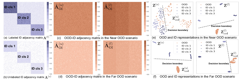
Figure 2: Example showcasing the contrast between adjacency matrices and representations w/ (l) and w/o (u) ID labels. (a) The ID adjacency matrix in the labeled case $\mathbf{A}^{(l)}$. (b) The ID adjacency matrix in the unlabeled case $\mathbf{A}^{(u)}$. Here darker color indicates denser connectivity. The contrast of the OOD-ID adjacency matrix $\tilde{\mathbf{A}}_{\rm OI}$ w/ and w/o ID labels in the near OOD and far OOD scenario is shown in (c) and (d), where the adjacency matrices have a larger Frobenius norm, i.e., $\|\tilde{\mathbf{A}}_{\rm OI}^{(u)}\|_{F}=60$ in the near OOD scenario and smaller norm in the far OOD scenario, i.e., $\|\tilde{\mathbf{A}}_{\rm OI}^{(u)}\|_{F}=24$. (e) Learned representations in the near OOD scenario, where the OOD representations are overlapped in the unlabeled case but become linearly separable from the ID representations in the labeled case. (d) Representations in the far OOD scenario. The ID and OOD representations can already be separable in the unlabeled case. The benefit of ID labels is marginal.

OOD representations.

In post hoc OOD detection, the learning algorithm can only observe ID data in $\mathcal{X}_{\rm id}$ and the corresponding adjacency matrix. Hence, a key challenge in our framework is how to derive the OOD representations based on ID and OOD data connectivity in the input space. Unlike previous literature (Lee et al., 2018b), we refrain from making simplified assumptions in the feature representation space (although that makes analysis much easier). More realistically, we characterize OOD data directly in the input space by the adjacency matrix $\tilde{\mathbf{A}}_{\rm OI}^{(l)}\in\mathbb{R}^{M\times N}$, where $M$ is the number of OOD data points.

Each row in the matrix indicates the similarity between an OOD data w.r.t. all the ID samples. Depending on the characteristics of the OOD data, this matrix may be sparse if OOD data is far away from all the ID samples (e.g., far OOD), or can have dense entries if it is close to some ID classes (e.g., near OOD). Our characterization is thus general enough to enable analysis under different scenarios.

Now a question remains: how do we go from this matrix $\tilde{\mathbf{A}}_{\rm OI}^{(l)}$ to a $k$-dimensional embedding for each OOD data? While a naive solution is to perform spectral decomposition on the stack of two matrices $\tilde{\mathbf{A}}_{\rm OI}^{(l)}$ and $\tilde{\mathbf{A}}^{(l)}$, this violates the principle of post hoc OOD detection as it incurs retraining. Instead, we derive the embeddings of OOD vertices using existing ID embeddings $\mathbf{F}^{(l)}$ and the OOD-ID similarity. This can be achieved by solving the following optimization:

$$\min_{\mathbf{F}_{\rm ood}^{(l)}\in\mathbb{R}^{M\times k}}\left\|\tilde{\mathbf{A}}_{\rm OI}^{(l)}-\mathbf{F}_{\rm ood}^{(l)}\mathbf{F}^{(l)\top}\right\|_{F}^{2},$$ (7)

where $\mathbf{F}_{\rm ood}^{(l)}$ denotes the OOD embeddings. Intuitively, the objective distills the similarity in the input space into the representation space. For instance, it searches for an OOD representation, aligning it closely with ID representations when there is a dense connectivity between OOD and ID data in the adjacency matrix, and vice versa. Similar to the ID case, we have $\mathbf{Z}_{\rm ood}^{(l)}=[{\mathbf{D}_{\rm ood}^{(l)}}]^{-\frac{1}{2}}\mathbf{F}_{\rm ood}^{(l)}$, where $\mathbf{D}_{\rm ood}^{(l)}$ can be calculated in the same way as $\mathbf{D}^{(l)}$ based on $\tilde{\mathbf{A}}_{\rm OI}^{(l)}$. Therefore, the analytic form of the OOD representations from the neural network can be derived as

$$\mathbf{Z}_{\rm ood}^{(l)}=[\mathbf{D}_{\rm ood}^{(l)}]^{-\frac{1}{2}}\tilde{\mathbf{A}}_{\rm OI}^{(l)}\mathbf{V}_{k}^{(l)}[\mathbf{\Sigma}_{k}^{(l)}]^{-\frac{1}{2}}.$$ (8)

Detailed proof and the design rationale are in Appendix D.2.

Representation in the unlabeled case.

For the unlabeled case, we can get the representations for ID and OOD data by replacing the matrices $\mathbf{V}_{k}^{(l)},\mathbf{\Sigma}_{k}^{(l)},\mathbf{D}^{(l)},\mathbf{D}_{\rm ood}^{(l)}$ and $\tilde{\mathbf{A}}_{\rm OI}^{(l)}$ in Equations 6 and 8 with the unlabeled version. We will show how the labeled and unlabeled representations are rigorously related in Appendix C.1.

An illustrative example.

To contrast the adjacency matrices and the corresponding representations for the unlabeled and labeled cases, we simulate an example in Figure 2. The simulation is constructed with simplicity in mind, to facilitate understanding. Evaluations on complex high-dimensional data will be provided in Section 5. In particular, we base our analysis on the ID adjacency matrix as depicted in Figure 2 (a) and (b), which consists of three ID classes and 40 data points for each class. In the labeled case, the ID adjacency matrix has a denser connectivity pattern, especially for data that belongs to the same ID label. In Figure 2 (c) and (d), we compare the OOD-ID adjacency matrices with and without ID labels in two scenarios, i.e., near OOD where there are dense connections in $\tilde{\mathbf{A}}_{\rm OI}$ and far OOD where the connectivity in $\tilde{\mathbf{A}}_{\rm OI}$ is sparse.

Based on the graph, we further visualize in Figures 2 (e) and (f) the 2D data representations ($k=2$, calculated by Equations 6 and 8) for the near OOD and far OOD scenarios. We observe that having different adjacency matrices can lead to significantly different data representations. We will provide theory to rigorously analyze the OOD detection performance and contrast between the labeled and unlabeled cases (Section 4.3). Details of the illustrative example are included in Appendix F.

4.2 Evaluation Target

With the closed-form representations for both ID and OOD, we evaluate OOD detection by linear probing error. The strategy is commonly used in representation learning (Chen et al., 2020). Specifically, the weight of a linear classifier is denoted as $\boldsymbol{\theta}\in\mathbb{R}^{k\times 2}$. The class prediction (ID vs. OOD) is given by $\mathbf{g}_{\boldsymbol{\theta}}(\mathbf{z})={\rm argmax}_{i\in\{+,-\}}(\mathbf{h}_{\mathbf{w}}(\mathbf{x})\boldsymbol{\theta})_{i}$. Denote the set of ID and OOD features as ${\mathbf{Z}}_{\rm all}\in\mathbb{R}^{(N+M)\times k}=[\mathbf{Z}^{\top},\mathbf{Z}_{\rm ood}^{\top}]^{\top}$ (either labeled (u) or unlabeled (l)), the linear probing error $R({\mathbf{Z}}_{\rm all})$ is given by the least error of all possible linear classifiers:

$$R({\mathbf{Z}}_{\rm all})\triangleq\min_{\boldsymbol{\theta}\in\mathbb{R}^{k\times 2}}\mathbb{E}_{\mathbf{z}\in{\mathbf{Z}}_{\rm all}}\mathds{1}[y(\mathbf{z})\neq\mathbf{g}_{\boldsymbol{\theta}}(\mathbf{z})],$$ (9)

where $y(\mathbf{z})$ denotes indicates the ground-truth class of feature $\mathbf{z}$ (ID or OOD). With the definition, we can bound the linear probing error $R({\mathbf{Z}}_{\rm all})$ by the residual of the regression error as shown in Lemma 2 with proof in Appendix D.3.

Lemma 2.

Denote $\mathbf{y}\in\mathbb{R}^{(N+M)\times 2}$ as a matrix where each row contains the one-hot label for features in ${\mathbf{Z}}_{\rm all}$. We have:

$$R({\mathbf{Z}}_{\rm all})\leq\frac{2}{N+M}\operatorname{Tr}\left(\left(\mathbf{I}-{\mathbf{Z}}_{\rm all}{\mathbf{Z}}_{\rm all}^{\dagger}\right)\mathbf{y}\mathbf{y}^{\top}\right).$$ (10)

Here $\operatorname{Tr}\left(\cdot\right)$ denotes the trace operator. ${\mathbf{Z}}_{\rm all}^{\dagger}$ is the Moore-Penrose inverse of matrix ${\mathbf{Z}}_{\rm all}$. We denote this upper bound as $\overline{R}({\mathbf{Z}}_{\rm all})$, which is more tractable to analyze and behaves similarly to $R({\mathbf{Z}}_{\rm all})$ as shown in Appendix D.3. Therefore our subsequent analysis revolves around it.

4.3 Error Bound on OOD Detection Performance

With the evaluation target defined above, we now present the formal error bound on OOD detection performance by contrasting the labeled and unlabeled cases. As an overview, Theorem 1 will present the lower bound of linear probing error difference between the unlabeled and label case, along with an intuitive version in Theorem 2. We specify several mild assumptions and necessary notations for our theorems in Appendix A. Due to space limitation, we omit unimportant constants and simplify the statements of our theorems. We defer the full formal statements in Appendix B. All proofs can be found in Appendix C.

Error difference between unlabeled and labeled cases.

Formally, we investigate the following linear probing error difference between the unlabeled and labeled case:

$$\mathcal{G}=\overline{R}({\mathbf{Z}}_{\rm all}^{(u)})-\overline{R}({\mathbf{Z}}_{\rm all}^{(l)}),$$ (11)

where a larger error difference indicates that labeled ID data benefits OOD detection more substantially, and vice versa. The lower bound on $\mathcal{G}$ is given by the following theorem.

Theorem 1 (Lower bound of the linear probing error difference w/ and w/o ID labels).

(Informal.) Suppose we have adjacency matrices $\tilde{\mathbf{A}}^{(u)},\tilde{\mathbf{A}}^{(l)}\in\mathbb{R}^{N\times N}$ and $\tilde{\mathbf{A}}_{\rm OI}^{(u)},\tilde{\mathbf{A}}_{\rm OI}^{(l)}\in\mathbb{R}^{M\times N}$ for both the labeled and unlabeled cases. Under mild conditions, given positive constants $\phi_{l},C$, the error difference $\mathcal{G}$ in Equation 11 is lower bounded by

$$\mathcal{G} \geq\frac{C\phi_{l}}{N+M}\epsilon(\mathfrak{p},\mathfrak{q},\tilde{\mathbf{A}}^{(u)},\tilde{\mathbf{A}}_{\rm OI}^{(u)}),$$ (12)

where $\mathfrak{q}\in\mathbb{R}^{N\times c}$ with each column defined as $(\mathfrak{q}_{i})_{\mathbf{x}}=\mathbb{E}_{\bar{\mathbf{x}}_{l}\sim{\mathbb{P}_{l_{i}}}}\mathcal{T}(\mathbf{x}|\bar{\mathbf{x}}_{l}),\mathbf{x}\in\mathcal{X}_{\rm id}$. Similarly, $\mathfrak{p}\in\mathbb{R}^{M\times c}$ is defined as $(\mathfrak{p}_{i})_{\mathbf{x}}=\mathbb{E}_{\bar{\mathbf{x}}_{l}\sim{\mathbb{P}_{l_{i}}}}\mathcal{T}(\mathbf{x}|\bar{\mathbf{x}}_{l}),\mathbf{x}\in\mathcal{X}_{\rm ood}$. Semantically, each entry in $\mathfrak{q}$ means the connection magnitude from $\mathbf{x}$ to all ID data while each entry in $\mathfrak{p}$ is the connection from $\mathbf{x}$ to OOD data. Furthermore,

$$\epsilon(\mathfrak{p},\mathfrak{q},\tilde{\mathbf{A}}^{(u)},\tilde{\mathbf{A}}_{\rm OI}^{(u)})=2\sum_{i=1}^{c}\operatorname{Tr}\left(\mathfrak{p}_{i}\mathfrak{q}_{i}^{\top}\cdot\tilde{\mathbf{A}}_{\rm OI}^{(u)\top}\right)+$$

$$\left(1-\|\tilde{\mathbf{A}}_{\rm OI}^{(u)}\|_{F}^{2}\|\tilde{\mathbf{A}}^{(u)}\|_{F}^{2}\right)\sum_{i=1}^{c}\|\mathfrak{q}_{i}\|_{F}^{2}+$$

$$r^{2}\left(\|\tilde{\mathbf{A}}_{\rm OI}^{(u)}\|_{F}^{2}\|\tilde{\mathbf{A}}^{(u)}\|_{F}^{2}\frac{2(\tau-k)}{\tau-1}-2\right)\cdot\sum_{i=1}^{c}\|\mathfrak{q}_{i}\|_{1},$$

where $\tau$ is a constant that measures the $k$-th spectral gap of matrix $\tilde{\mathbf{A}}^{(u)}$, i.e., $\boldsymbol{\lambda}_{k}^{(u)}\geq\tau\boldsymbol{\lambda}_{k+1}^{(u)}$ and $\boldsymbol{\lambda}_{k}^{(u)}$ is the $k$-th largest singular value of $\tilde{\mathbf{A}}^{(u)}$. $r$ is the maximum $l_{2}$ norm of the ID representations, i.e., $r=\max_{\mathbf{z}\in\mathbf{Z}^{(u)}}\|\mathbf{z}\|_{2}$.

Theorem 1 is a general characterization of the error difference in the labeled and unlabeled cases. To gain a better insight, we introduce Theorem 2 which provides intuition interpretations.

OOD category	OOD dataset	ID labels	FPR95$\downarrow$	AUROC$\uparrow$	LP error$\downarrow$	FPR95$\downarrow$	AUROC$\uparrow$	LP error$\downarrow$
			$\mathbb{P}_{\rm ood}^{\rm test}=\mathbb{P}_{\rm ood}^{\rm LP}$			$\mathbb{P}_{\rm ood}^{\rm test}\neq\mathbb{P}_{\rm ood}^{\rm LP}$
Far OOD	Svhn	-	0.09±0.02	99.96±0.01	0.02±0.00	75.62±4.74	77.09±2.17	0.52±0.21
		+	0.07±0.00	99.97±0.03	0.02±0.00	68.73±5.03	82.97±1.87	0.48±0.28
	Textures	-	0.37±0.20	99.80±0.15	0.02±0.00	86.35±2.47	70.94±3.77	1.05±0.17
		+	0.24±0.19	99.86±0.11	0.01±0.00	86.44±0.58	75.15±3.36	0.95±0.10
	Places365	-	0.68±0.10	99.98±0.00	0.02±0.01	75.35±2.78	79.85±1.85	0.83±0.27
		+	0.44±0.06	99.99±0.01	0.02±0.01	66.60±1.61	85.03±3.19	0.74±0.09
	Lsun-Resize	-	0.24±0.03	99.95±0.03	0.02±0.00	83.57±2.89	77.57±5.21	0.84±0.21
		+	0.24±0.01	99.91±0.07	0.02±0.01	74.13±4.95	82.71±1.64	0.75±0.14
	Lsun-C	-	1.68±0.36	99.20±0.17	0.05±0.01	63.42±6.16	83.43±3.48	0.82±0.38
		+	1.04±0.41	99.35±0.08	0.04±0.02	51.36±2.26	89.49±1.91	0.72±0.41
Near OOD	Cifar10	-	62.20±3.49	85.93±1.72	0.27±0.11	94.54±0.79	55.42±1.64	0.97±0.18
		+	58.28±2.90	89.01±0.98	0.19±0.05	91.07±3.28	67.72±0.97	0.85±0.32

Table 1: OOD detection results w/ and w/o ID labels (Cifar100 as ID). Mean and std are estimated on three different runs. Better results are highlighted in bold. “+,-” denotes the labeled and unlabeled case. “LP error” denotes the error of linear probing. $\uparrow$ indicates larger values are better, and $\downarrow$ indicates smaller values are better. The table shows that (1) the ID labeling information helps OOD detection, especially in the near OOD scenario and when $\mathbb{P}_{\rm ood}^{\rm test}=\mathbb{P}_{\rm ood}^{\rm LP}$; Moreover, our observations can generalize to the case where the OOD distribution in linear probing is not the same as that in actual testing ($\mathbb{P}_{\rm ood}^{\rm test}\neq\mathbb{P}_{\rm ood}^{\rm LP}$), showcasing the generality of our theory.

Interpretation and key insights.

Theorem 2 shows that the optimal scenarios for achieving the greatest reduction in linear probing error—signifying the most significant benefit by incorporating the ID labels, are when

1. The ID data are connected sparsely in the unlabeled case (i.e., $\|\tilde{\mathbf{A}}^{(u)}\|_{F}^{2}<2N^{2}$), which always holds because $\|\tilde{\mathbf{A}}^{(u)}\|_{\infty}<N$;

2. The OOD data is closely connected to the ID data (near OOD, i.e., $\|\tilde{\mathbf{A}}_{\rm OI}^{(u)}\|_{F}^{2}$ is relatively large);

3. The semantic connection between each ID data to the labeled ID data from different ID classes is sufficiently large (i.e., $\|\mathfrak{q}\|_{F}^{2}$ is large).

Moreover, the simplified bound also enables us to interpret the relationship of each key component with the error reduction $\mathcal{G}$. For example, 1) the bound will monotonically increase when the connection within ID data in the unlabeled case becomes sparser (i.e., $\|\tilde{\mathbf{A}}^{(u)}\|_{F}^{2}$ $\downarrow$); 2) Since $\|\tilde{\mathbf{A}}^{(u)}\|_{F}^{2}$ is smaller than $2N^{2}$, strengthening the semantic connection from each ID data to the labeled data from different ID classes (i.e., $\|\mathfrak{q}\|_{F}^{2}$ $\uparrow$) is always helpful. Intuitively, a larger $\|\mathfrak{q}\|_{F}^{2}$ means one ID data point is more likely to be augmented from another ID data; 3) If the ID and OOD data are closer ($\|\tilde{\mathbf{A}}_{\rm OI}^{(u)}\|_{F}^{2}$ $\uparrow$), the value of the bound will increase given the same $\mathfrak{q}$ and $\tilde{\mathbf{A}}^{(u)}$.

Verification of bound on the illustrative example.

Our theoretical guarantee aligns well with the empirical results. For example, in Figure 2 (e) where the OOD data is densely connected to the ID data (near OOD case), the ID labels can better shape the ID and OOD representations compared to the unlabeled case, rendering them linearly separable. As a result, the linear probing error is reduced from 0.09 in the unlabeled case to 0 in the labeled case. In contrast, when the OOD data is far from the ID data (Figure 2 (f)), the representations for ID and OOD are already well separated in the unlabeled case, and thus the benefit of ID labels is relatively marginal. As a verification, the linear probing error remains 0 both with and without ID labels. Therefore, these observations align with our key insight on the effect of OOD-ID connection $\tilde{\mathbf{A}}_{\rm OI}^{(u)}$ on the error difference for linear probing. Moreover, we provide additional visualization results on changing the Frobenius norm of the ID adjacency matrix $\tilde{\mathbf{A}}^{(u)}$ and the semantic connection $\mathfrak{q}$ in Appendix G.

5 Experiments on Real Datasets

In this section, we verify our theoretical results using real-world OOD detection benchmarks.

Experimental setup.

For ID datasets, we use Cifar10 and Cifar100 (Krizhevsky et al., 2009). We first train the neural network on the ID data for 200 epochs with a ResNet-18 (He et al., 2016), using objective $\mathcal{L}_{\text{unlabeled}}$ and $\mathcal{L}_{\text{labeled}}$ for the unlabeled and labeled case, respectively. The penultimate layer embedding dimension $k=512$. We then extract the embeddings for the ID and OOD data and perform linear probing (50 epochs). We explore two different scenarios depending on whether the OOD in linear probing ($\mathbb{P}_{\rm ood}^{\rm LP}$) is the same as the test OOD ($\mathbb{P}_{\rm ood}^{\rm test}$). In the first scenario ($\mathbb{P}_{\rm ood}^{\rm test}=\mathbb{P}_{\rm ood}^{\rm LP}$), we use 75% of the OOD dataset for linear probing and the remaining for testing. Specifically, for far OOD test datasets, we use a suite of natural image datasets including Textures (Cimpoi et al., 2014), Svhn (Netzer et al., 2011), Places365 (Zhou et al., 2017), and Lsun (Yu et al., 2015). For near OOD, we evaluate on Cifar10 when Cifar100 is ID and vice versa. In the second scenario ($\mathbb{P}_{\rm ood}^{\rm test}\neq\mathbb{P}_{\rm ood}^{\rm LP}$), we use 300K Random Images (Hendrycks et al., 2019) for linear probing and the other OOD datasets for evaluation. More experiment details are in Appendix H.

Evaluation metrics.

We report the following metrics: (1) the false positive rate (FPR95$\downarrow$) of OOD samples when the true positive rate of ID samples is 95%, (2) the area under the receiver operating characteristic curve (AUROC$\uparrow$), and (3) the linear probing error (LP error $\downarrow$).

Experiment results.

The results are shown in Table 1, which demonstrate that: (1) the ID labeling information helps OOD detection, especially in the near OOD scenario and when $\mathbb{P}_{\rm ood}^{\rm test}=\mathbb{P}_{\rm ood}^{\rm LP}$. For example, the AUROC is improved by 3.08% on Cifar10 compared to 0.02% on Svhn, echoing our theoretical insights; (2) Our observations can generalize to the case where the OOD distribution in linear probing is not the same as that in actual testing ($\mathbb{P}_{\rm ood}^{\rm test}\neq\mathbb{P}_{\rm ood}^{\rm LP}$), where the AUROC increases by 12.3% compared to the unsupervised counterpart on Cifar10, showcasing the flexibility and generality of our theory. Additional results on Cifar10 as the ID dataset and the evaluation using post-hoc OOD detection score are shown in Appendix I.

Verification of bound.

We verify the error difference $\mathcal{G}$ and its relationship to the Frobenius norm of the adjacency matrices $\tilde{\mathbf{A}}^{(u)}$ and $\tilde{\mathbf{A}}_{\rm OI}^{(u)}$. Firstly, to verify how the value of $\mathcal{G}$ will change given a larger Frobenius norm of $\tilde{\mathbf{A}}_{\rm OI}^{(u)}$, we compare the linear probing error on Svhn and Cifar10 in Table 2 with and without ID labels, where the error difference on Cifar10 (near OOD, with larger $\|\tilde{\mathbf{A}}_{\rm OI}^{(u)}\|_{F}$) is consistently larger than that on Svhn (far OOD).

OOD dataset	Svhn	C10
	Far OOD	Near OOD
$\|\tilde{\mathbf{A}}_{\rm OI}^{(u)}\|_{F}$ $\uparrow$	$2334$	$2739$
$\mathcal{G}$ $\uparrow$	0.00	0.08

Table 2: Verification with different $\|\tilde{\mathbf{A}}_{\rm OI}^{(u)}\|_{F}$ (Cifar100 as ID).

In addition, we verify the relationship of $\|\tilde{\mathbf{A}}^{(u)}\|_{F}$ and the error difference (Cifar10 as OOD) in Table 3. Specifically, we calculate the norm of the ID adjacency matrix from different training epochs and observe that the difference in linear probing error tends to increase with decreasing $\|\tilde{\mathbf{A}}^{(u)}\|_{F}$, which aligns with Theorem 2. Additional results and details are included in Appendix E. We further analyze the tightness of our bound in Appendix J.

Epochs	40	80	120	160	200	240
$\|\tilde{\mathbf{A}}^{(u)}\|_{F}$ $\downarrow$	20191	19549	18939	16073	15509	14810
$\mathcal{G}$ $\uparrow$	0.01	0.03	0.06	0.06	0.08	0.09

Table 3: Verification with different $\|\tilde{\mathbf{A}}^{(u)}\|_{F}$ (Cifar100 as ID).

6 Related Work

OOD detection

has attracted a surge of interest in recent years (Fort et al., 2021; Yang et al., 2021b; Fang et al., 2022; Zhu et al., 2022; Ming et al., 2022a, c; Yang et al., 2022; Wang et al., 2022b; Galil et al., 2023; Djurisic et al., 2023; Zheng et al., 2023; Wang et al., 2022a, 2023b; Narasimhan et al., 2023; Yang et al., 2023; Uppaal et al., 2023; Zhu et al., 2023b, a; Ming & Li, 2023; Zhang et al., 2023; Ghosal et al., 2024). One line of work performs OOD detection by devising scoring functions, including confidence-based methods (Bendale & Boult, 2016; Hendrycks & Gimpel, 2017; Liang et al., 2018), energy-based score (Liu et al., 2020b; Wang et al., 2021; Wu et al., 2023), distance-based approaches (Lee et al., 2018b; Tack et al., 2020; Ren et al., 2021; Sehwag et al., 2021a; Sun et al., 2022; Du et al., 2022a; Ming et al., 2023; Ren et al., 2023), gradient-based score (Huang et al., 2021), and Bayesian approaches (Gal & Ghahramani, 2016; Lakshminarayanan et al., 2017; Maddox et al., 2019; Malinin & Gales, 2019; Wen et al., 2020; Kristiadi et al., 2020). Another line of work addressed OOD detection by training-time regularization (Bevandić et al., 2018; Malinin & Gales, 2018; Geifman & El-Yaniv, 2019; Hein et al., 2019; Meinke & Hein, 2020; Jeong & Kim, 2020; Liu et al., 2020a; van Amersfoort et al., 2020; Yang et al., 2021a; Wei et al., 2022; Du et al., 2022b, 2023; Wang et al., 2023a). For example, the model is regularized to produce lower confidence (Lee et al., 2018a) or higher energy (Liu et al., 2020b; Du et al., 2022c) on a set of clean OOD data (Hendrycks et al., 2019; Ming et al., 2022b), wild data (Zhou et al., 2021; Katz-Samuels et al., 2022; He et al., 2023; Bai et al., 2023; Du et al., 2024) and synthetic outliers (Du et al., 2023; Tao et al., 2023; Park et al., 2023). Additionally, a similar topic in a different domain, i.e., anomaly detection, often restricts the ID (normality) to be with a single class and with a different definition of the outliers (Chandola et al., 2009; Han et al., 2022).

Most OOD detection methods rely on the supervision of ID labels, and there have been prior works, such as (Tack et al., 2020; Sehwag et al., 2021b; Sun et al., 2022) that empirically verified that training with the ID labels can achieve a much better OOD detection performance compared to the unsupervised version, but a provable analysis of their impact is critical yet missing in the field.

OOD detection theory.

Recent studies have begun to focus on the theoretical understanding of OOD detection.  Fang et al. (2022) studied the generalization of OOD detection by PAC learning and they found a necessary condition for the learnability of OOD detection. Morteza & Li (2022) derived a novel OOD score and provided a provable understanding of the OOD detection result using that score. Du et al. (2024) theoretically studied the impact of unlabeled data for OOD detection. In contrast, we formally analyze the impact of ID labels on OOD detection, which has not been studied in the past.

Spectral graph theory

is a classical research problem (Von Luxburg, 2007; Chung, 1997; Cheeger, 2015; Kannan et al., 2004; Lee et al., 2014; McSherry, 2001), which aims to partition the graph by studying the eigenspace of the adjacency matrix. Recently, it has been applied in different applications in machine learning (Ng et al., 2001; Shi & Malik, 2000; Blum, 2001; Zhu et al., 2003; Argyriou et al., 2005; Shaham et al., 2018). HaoChen et al. (2021) derived the spectral contrastive learning from the factorization of the graph’s adjacency matrix, and provably understand unsupervised domain adaptation (Shen et al., 2022; HaoChen et al., 2022). Sun et al. (2023a, b) expanded the spectral contrastive learning approach to novel class discovery and open-world semi-supervised learning. Our focus is on the OOD detection problem, which differs from prior literature.

7 Conclusion

In this paper, we propose a novel analytical framework that studies the impact of ID labels on OOD detection. Our framework takes a graph-theoretic approach by modeling the ID data via a graph, which allows us to characterize the feature representations by performing spectral decomposition on the graph that can be expressed equivalently as a contrastive learning objective on neural net representation. Leveraging these representations, we establish a provable error bound that compares the OOD detection performance with and without ID labels, which reveals sufficient conditions for achieving improved OOD detection performance. Empirical observations further support our theoretical conclusions, showcasing the benefits of ID labeling information under proper conditions. We hope our work will inspire future research on the theoretical understanding of OOD detection. One promising direction is to analyze the setting where there is access to OOD samples, which belongs to an important branch of work in OOD detection literature.

Impact Statement

Our paper aims to improve the reliability and safety of modern machine learning models. From the theoretical perspective, our analysis can facilitate and deepen the understanding of the effect of in-distribution labels for OOD detection. In Appendix E and Section 5 of the main paper, we properly verify the necessary conditions and the value of our bound using real-world datasets. Hence, we believe our theoretical framework has a broad utility and significance.

From the practical side, our study can lead to direct benefits and societal impacts by deploying OOD detection techniques, particularly when practitioners need to determine how to better leverage the in-distribution labels, such as in safety-critical applications i.e., autonomous driving and healthcare data analysis. Our study does not involve any human subjects or violation of legal compliance. We do not anticipate any potentially harmful consequences to our work. Through our study and releasing our code, we hope to raise stronger research and societal awareness on the safe handling of out-of-distribution data in real-world settings.

When and How Does In-Distribution Label Help Out-of-Distribution Detection?
(Appendix)

Appendix A Notations, Assumptions and Important Constants

Here we summarize the important notations and constants in Table 4, and restate necessary definitions and assumptions in Section A.2.

A.1 Notations

Please see Table 4 for detailed notations.

Table 4: Main notations and their descriptions.

Notation	Description
Spaces
$\mathcal{X}$, $\mathcal{Z}$, $\mathcal{Y}$	the input, representation space and the label space.
Distributions
$\mathbb{P}_{{\rm id}}$, $\mathbb{P}_{{\rm ood}}$	data distribution for ID data and OOD data
$\mathbb{P}_{\mathcal{X}\mathcal{Y}}$	the joint data distribution for ID data.
Data and Models
$\mathbf{x}$	input to the neural network
$\tilde{\mathbf{A}}_{\rm OI}^{(u)}$ and $\tilde{\mathbf{A}}_{\rm OI}^{(l)}$	adjacency matrix between OOD and ID data in the labeled and unlabeled case
$\mathbf{A}^{(u)}$ and $\mathbf{A}^{(l)}$	adjacency matrix for ID data in the labeled and unlabeled case
$\tilde{\mathbf{A}}^{(u)}$ and $\tilde{\mathbf{A}}^{(l)}$	normalized adjacency matrix for ID data in the labeled and unlabeled case
$\mathbf{D}^{(u)}$ and $\mathbf{D}^{(l)}$	ID diagonal matrix with the diagonal elements being the row sum of $\mathbf{A}^{(u)}$ and $\mathbf{A}^{(l)}$.
$\mathbf{D}^{(u)}_{\rm ood}$ and $\mathbf{D}^{(l)}_{\rm ood}$	OOD diagonal matrix with the diagonal elements being the row sum of $\tilde{\mathbf{A}}_{\rm OI}^{(u)}$ and $\tilde{\mathbf{A}}_{\rm OI}^{(l)}$.
$\mathcal{T}$	augmentation graph
$\mathbf{w}$, $\boldsymbol{\theta}$	weight of the ID feature extractor and the linear probing layer
$\mathbf{h}_{\mathbf{w}}$ and $\mathbf{g}_{\boldsymbol{\theta}}$	feature extractor on ID data and linear probing layer for OOD detection
$y$, $\mathbf{y}$	binary label for linear probing, vectorized one-hot label for $y$
$\mathbf{z}$	feature for single input $\mathbf{x}$
$\mathbf{Z}^{(u)}$ and $\mathbf{Z}^{(l)}$	representation matrix for ID data in the labeled and unlabeled case
$\mathbf{Z}_{\rm ood}^{(u)}$ and $\mathbf{Z}_{\rm ood}^{(l)}$	representation matrix for OOD data in the labeled and unlabeled case
$\mathbf{Z}_{\rm all}^{(u)}$ and $\mathbf{Z}_{\rm all}^{(l)}$	representation matrix for both ID and OOD data in the labeled and unlabeled case
$\mathfrak{q}$ and $\mathfrak{p}$	semantic connection from each ID/OOD data to the labeled ID data.
$N$, $M$	size of $\mathbf{Z}$, size of $\mathbf{Z}_{\rm ood}$
$\boldsymbol{\lambda}$	eigenvalue vector of $\tilde{\mathbf{A}}$
$\mathbf{v}_{j}$	the $j$-th eigenvector of $\tilde{\mathbf{A}}$
$\mathbf{V}_{k},\mathbf{V}_{\varnothing}$	the first $k$ eigenvectors of $\tilde{\mathbf{A}}$/the latter $N-k$ eigenvectors of $\tilde{\mathbf{A}}$ (null space of $\mathbf{V}_{k}$)
Distances
$\|\cdot\|_{1},\|\cdot\|_{2},\|\cdot\|_{F}$	$\ell_{1},\ell_{2}$ norm and Frobenius norm
Loss and Risk
$\mathcal{L}_{\rm unlabeled}(\cdot),\mathcal{L}_{\rm labeled}(\cdot)$	ID loss function in the unlabeled and labeled case
$R({\mathbf{Z}_{\rm all}})$	the empirical risk w.r.t. linear probing module over feature set $\mathbf{Z}_{\rm all}$
$\overline{R}({\mathbf{Z}_{\rm all}})$	the upper bound of $R(\mathbf{Z}_{\rm all})$
$\mathcal{G}$	linear probing error difference with and without ID labels
Constants
$\phi_{u},\phi_{l}$	weight coefficients for the unlabeled and labeled case.
$k$	dimension of the feature representation
$\tau$	the parameter that measures the eigengap of $\tilde{\mathbf{A}}^{(u)}$
$r$	the maximum $\ell_{2}$ norm of the ID features, i.e., $r=\max_{\mathbf{z}\in\mathbf{Z}^{(u)}}\|\mathbf{z}\|_{2}$
$C$	constants in Theorem 1

A.2 Assumptions

Assumption 1 (Property of ID adjacency matrix).

We assume the adjacency matrix $\tilde{\mathbf{A}}^{(u)}$ has the following property: There exists a positive constant $k\leq N$ such that the $k$-th eigengap of $\tilde{\mathbf{A}}^{(u)}$ satisfies that $\boldsymbol{\lambda}_{k}^{(u)}\geq\tau\boldsymbol{\lambda}_{k+1}^{(u)},\tau>k$, where $\boldsymbol{\lambda}_{k}^{(u)}$ is the $k$-th largest eigenvalue of matrix $\tilde{\mathbf{A}}^{(u)}$.

Remark 1.

We have empirically verified our assumption using both simulated and real-world datasets in Section E.

Assumption 2 (Property of vectors that depict the semantic connection between each ID/OOD data to the labeled ID data).

Similar to (Sun et al., 2023a), we assume each row of the matrix $\mathfrak{q}$ lies in the linear span of $\mathbf{V}_{k}^{(u)}$ and $\mathbf{V}_{k}^{(u)}[\mathbf{\Sigma}_{k}^{(u)}]^{-\frac{1}{2}}$, i.e., $\mathbf{V}_{\varnothing}^{(u)\top}\mathfrak{q}_{i}=0,\mathbf{V}_{k}^{(u)}\mathbf{V}_{k}^{(u)\top}\mathfrak{q}_{i}=\mathfrak{q}_{i}$ and $\mathbf{V}_{k}^{(u)}[\mathbf{\Sigma}_{k}^{(u)}]^{-1}\mathbf{V}_{k}^{(u)\top}\mathfrak{q}_{i}=\mathfrak{q}_{i}$.

Remark 2.

Following the assumptions made in the existing literature (Sun et al., 2023a), the assumption is used to simplify $\mathbf{V}_{k}^{(u)}\mathbf{V}_{k}^{(u)\top}\mathfrak{q}_{i}\mathfrak{q}_{i}^{\top}\mathbf{V}_{\varnothing}^{(u)}\mathbf{V}_{\varnothing}^{(u)\top}+\mathbf{V}_{k}^{(u)}\mathbf{V}_{k}^{(u)\top}\mathfrak{q}_{i}\mathfrak{q}_{i}^{\top}$ to $\mathfrak{q}_{i}\mathfrak{q}_{i}^{\top}$ and simplify $\mathbf{V}_{k}^{(u)}[\mathbf{\Sigma}_{k}^{(u)}]^{-1}\mathbf{V}_{k}^{(u)\top}\mathfrak{q}_{i}$ to $\mathfrak{q}_{i}$.

Appendix B Main Theorems

In this section, we provide a detailed and formal version of our main theorems with a complete description of the constant terms and other additional details that are omitted in the main paper.

Theorem 1 (Lower bound of the error difference between unlabeled and labeled cases, recap of Theorem 1 in the main paper).

Suppose we have adjacency matrices $\tilde{\mathbf{A}}^{(u)},\tilde{\mathbf{A}}^{(l)}\in\mathbb{R}^{N\times N}$ and $\tilde{\mathbf{A}}_{\rm OI}^{(u)},\tilde{\mathbf{A}}_{\rm OI}^{(l)}\in\mathbb{R}^{M\times N}$ for both the labeled and unlabeled cases. If Assumption 2 holds, given positive constants $\phi_{l},C$, the error difference $\mathcal{G}$ in Equation 11 is bounded by

$$\mathcal{G}\geq\frac{C\phi_{l}}{N+M}\epsilon(\mathfrak{p},\mathfrak{q},\tilde{\mathbf{A}}^{(u)},\tilde{\mathbf{A}}_{\rm OI}^{(u)}),$$ (13)

where $\mathfrak{q}\in\mathbb{R}^{c\times N}$ with each row being defined as $(\mathfrak{q}_{i})_{\mathbf{x}}=\mathbb{E}_{\bar{\mathbf{x}}_{l}\sim{\mathbb{P}_{l_{i}}}}\mathcal{T}(\mathbf{x}|\bar{\mathbf{x}}_{l}),\mathbf{x}\in\mathcal{X}_{\rm id}$. Similarly, we have $\mathfrak{p}\in\mathbb{R}^{c\times M}$ and $(\mathfrak{p}_{i})_{\mathbf{x}}=\mathbb{E}_{\bar{\mathbf{x}}_{l}\sim{\mathbb{P}_{l_{i}}}}\mathcal{T}(\mathbf{x}|\bar{\mathbf{x}}_{l}),\mathbf{x}\in\mathcal{X}_{\rm ood}$. Furthermore,

$$\epsilon(\mathfrak{p},\mathfrak{q},\tilde{\mathbf{A}}^{(u)},\tilde{\mathbf{A}}_{\rm OI}^{(u)}) =2\sum_{i=1}^{c}\operatorname{Tr}\left(\mathfrak{p}_{i}\mathfrak{q}_{i}^{\top}\cdot\tilde{\mathbf{A}}_{\rm OI}^{(u)\top}\right)+\left(1-\|\tilde{\mathbf{A}}_{\rm OI}^{(u)}\|_{F}^{2}\|\tilde{\mathbf{A}}^{(u)}\|_{F}^{2}\right)\sum_{i=1}^{c}\|\mathfrak{q}_{i}\|_{F}^{2}+$$ (14)

$$r^{2}\left(\|\tilde{\mathbf{A}}_{\rm OI}^{(u)}\|_{F}^{2}\|\tilde{\mathbf{A}}^{(u)}\|_{F}^{2}\frac{2(\tau-k)}{\tau-1}-2\right)\cdot\sum_{i=1}^{c}\|\mathfrak{q}_{i}\|_{1},$$

where $\tau$ is a constant that measures the $k$-th spectral gap of matrix $\tilde{\mathbf{A}}^{(u)}$, i.e., $\boldsymbol{\lambda}_{k}^{(u)}\geq\tau\boldsymbol{\lambda}_{k+1}^{(u)}$ and $\boldsymbol{\lambda}_{k}^{(u)}$ is the $k$-th largest singular value of $\tilde{\mathbf{A}}^{(u)}$. $r$ is the maximum $l_{2}$ norm of the ID representations, i.e., $r=\max_{\mathbf{z}\in\mathbf{Z}^{(u)}}\|\mathbf{z}\|_{2}$.

  

Theorem 2 (Simplified version of Theorem 1, recap of Theorem 2 in the main paper).

Under the same conditions in Theorem 1, if the number of ID and OOD samples $N$ and $M$ is sufficiently large, assume the $k$-th spectral gap of $\tilde{\mathbf{A}}^{(u)}$ satisfies $\tau>k$ (Assumption 1 holds), then the main error component $\epsilon(\mathfrak{p},\mathfrak{q},\tilde{\mathbf{A}}^{(u)},\tilde{\mathbf{A}}_{\rm OI}^{(u)})$ in Equation 14 satisfies

$$\epsilon(\mathfrak{p},\mathfrak{q}, \tilde{\mathbf{A}}^{(u)},\tilde{\mathbf{A}}_{\rm OI}^{(u)})\geq\left[1+\|\tilde{\mathbf{A}}_{\rm OI}^{(u)}\|_{F}^{2}\left(2N^{2}-\|\tilde{\mathbf{A}}^{(u)}\|_{F}^{2}\right)\right]\sum_{i=1}^{c}\|\mathfrak{q}_{i}\|_{F}^{2}.$$ (15)

Appendix C Proofs of Main Theorems

C.1 Proof of Theorem 1

Before proving Theorem 1, we first explain the framework introduced in Section 4 of the main paper to analyze the difference in the adjacency matrices and the corresponding feature representations between the unlabeled and labeled cases. Specifically, we proposed to analyze the adjacency matrix in the labeled case by perturbation analysis.

Matrix perturbation in the labeled case. Recall that we define in Definition 4 that the adjacency matrix in the labeled case (l) is the unlabeled one (u) plus connectivity incurred by the ID labels, which can be regarded as the perturbation of the labeling information. Therefore, for the ID adjacency matrix with ID labels, we have the perturbation on $\mathbf{A}^{(u)}$ as follows:

$$\mathbf{A}^{(l)}=\phi_{u}\mathbf{A}^{(u)}+\phi_{l}\Delta\mathbf{A},$$ (16)

where $\Delta\mathbf{A}\in\mathbb{R}^{N\times N}$ can be calculated based on the augmentation graph $\mathcal{T}$ according to Definition 4. Following (Sun et al., 2023a), we study the perturbation from two aspects: (1) The direction of the perturbation which is given by $\Delta\mathbf{A}$, (2) The perturbation magnitude $\phi_{l}$. We first consider the perturbation direction $\Delta\mathbf{A}$ and recall that we defined the concrete form in Definition 4:

$$[\Delta\mathbf{A}]_{\mathbf{x}\mathbf{x}^{\prime}}\triangleq\sum_{i\in\mathcal{Y}}\mathbb{E}_{\bar{\mathbf{x}}_{l}\sim\mathbb{P}_{l_{i}}}\mathbb{E}_{\bar{\mathbf{x}}_{l}^{\prime}\sim\mathbb{P}_{l_{i}}}\mathcal{T}\left(\mathbf{x}\mid\bar{\mathbf{x}}_{l}\right)\mathcal{T}\left(\mathbf{x}^{\prime}\mid\bar{\mathbf{x}}_{l}^{\prime}\right),\quad\mathbf{x},\mathbf{x}^{\prime}\in\mathcal{X}_{\rm id}$$ (17)

where $\mathcal{T}$ is the augmentation graph. In our theory, we consider $\|\mathcal{Y}\|=c$, and then we observe that $\Delta\mathbf{A}$ is the sum of $c$ rank-1 matrices, which can be written as:

$$\Delta\mathbf{A}=\sum_{i=1}^{c}\mathfrak{q}_{i}\mathfrak{q}_{i}^{\top},$$ (18)

where $\mathfrak{q}\in\mathbb{R}^{N\times c}$ with each column defined as $(\mathfrak{q}_{i})_{\mathbf{x}}=\mathbb{E}_{\bar{\mathbf{x}}_{l}\sim\mathbb{P}_{l_{i}}}\mathcal{T}\left(\mathbf{x}\mid\bar{\mathbf{x}}_{l}\right),\mathbf{x}\in\mathcal{X}_{\rm id}$ and $\bar{\mathbf{x}}_{l}$ is the labeled ID data with label $i$. And following (Sun et al., 2023a), we define the diagonal matrix $\mathbf{D}^{(l)}$ as follows:

$$\mathbf{D}^{(l)}=\phi_{u}\cdot\mathbf{D}^{(u)}+\sum_{i=1}^{c}\phi_{l}\cdot{\rm diag}(\mathfrak{q}_{i}).$$ (19)

Without losing the generality, we let $\phi_{u}\cdot{\rm diag}(\mathbf{1}_{N}^{\top}\mathbf{A}^{(u)})=\mathbf{I}_{N\times N}$, which means the ID nodes have equal degree in the unlabeled case. We then have:

$$\mathbf{D}^{(l)}\triangleq\operatorname{diag}\left(\mathbf{1}_{N}^{\top}\mathbf{A}^{(l)}\right)=\mathbf{I}_{N\times N}+\phi_{l}\cdot\sum_{i=1}^{c}{\rm diag}(\mathfrak{q}_{i}).$$ (20)

The perturbation function of representation. We then consider a more generalized form for the ID adjacency matrix $\mathbf{A}$:

$$\mathbf{A}(\phi_{l})=\phi_{u}\mathbf{A}^{(u)}+\phi_{l}\cdot\sum_{i=1}^{c}\mathfrak{q}_{i}\mathfrak{q}_{i}^{\top}.$$ (21)

For the perturbation on the OOD-ID adjacency matrix $\tilde{\mathbf{A}}_{\rm OI}$, we define $\mathfrak{p}\in\mathbb{R}^{M\times c}$ with each column defined as $(\mathfrak{p}_{i})_{\mathbf{x}}=\mathbb{E}_{\bar{\mathbf{x}}_{l}\sim\mathbb{P}_{l_{i}}}\mathcal{T}\left(\mathbf{x}\mid\bar{\mathbf{x}}_{l}\right),\mathbf{x}\sim\mathcal{X}_{\rm ood}$ and $\bar{\mathbf{x}}_{l}$ is the labeled ID data with label $l_{i}$. Similar to Equation 17, we can define the concrete perturbation formula for $\tilde{\mathbf{A}}_{\rm OI}$ as follows:

$$[\Delta\tilde{\mathbf{A}}_{\rm OI}]_{\mathbf{x}\mathbf{x}^{\prime}}\triangleq\sum_{i\in\mathcal{Y}}\mathbb{E}_{\bar{\mathbf{x}}_{l}\sim\mathbb{P}_{l_{i}}}\mathbb{E}_{\bar{\mathbf{x}}_{l}^{\prime}\sim\mathbb{P}_{l_{i}}}\mathcal{T}\left(\mathbf{x}\mid\bar{\mathbf{x}}_{l}\right)\mathcal{T}\left(\mathbf{x}^{\prime}\mid\bar{\mathbf{x}}_{l}^{\prime}\right),\quad\mathbf{x}^{\prime}\sim\mathcal{X}_{\rm id},\mathbf{x}\sim\mathcal{X}_{\rm ood}.$$ (22)

And we have:

$$\tilde{\mathbf{A}}_{\rm OI}(\phi_{l})=\phi_{u}\tilde{\mathbf{A}}_{\rm OI}^{(u)}+\phi_{l}\cdot\sum_{i=1}^{c}\mathfrak{p}_{i}\mathfrak{q}_{i}^{\top}.$$ (23)

Similarly, for the ID diagonal matrix $\mathbf{D}$, we have that:

$$\mathbf{D}(\phi_{l})=\mathbf{I}_{N\times N}+\phi_{l}\cdot\sum_{i=1}^{c}{\rm diag}(\mathfrak{q}_{i}).$$ (24)

In Equations 21 and 23, we treat the adjacency matrix as a function of the “labeling perturbation” magnitude $\phi_{l}$. It is clear that $\mathbf{A}(0)=\phi_{u}\mathbf{A}^{(u)}$ and $\tilde{\mathbf{A}}_{\rm OI}(0)=\phi_{u}\tilde{\mathbf{A}}_{\rm OI}^{(u)}$ which are the scaled adjacency matrices in the unlabeled case. When we let the adjacency matrix be a function of $\phi_{l}$, the normalized form, and the derived feature representation should also be the function of $\phi_{l}$. We proceed by defining these terms.

The normalized ID adjacency matrix is given by:

$$\tilde{\mathbf{A}}(\phi_{l})=\mathbf{D}(\phi_{l})^{-\frac{1}{2}}{\mathbf{A}}(\phi_{l})\mathbf{D}(\phi_{l})^{-\frac{1}{2}},$$ (25)

In addition, for in-distribution feature representation $\mathbf{Z}(\phi_{l})$, it is derived from the top-$k$ eigen components of $\tilde{\mathbf{A}}(\phi_{l})$. Specifically, we have:

$$\mathbf{Z}(\phi_{l})\mathbf{Z}(\phi_{l})^{\top}=\mathbf{D}(\phi_{l})^{-\frac{1}{2}}\tilde{\mathbf{A}}_{k}(\phi_{l})\mathbf{D}(\phi_{l})^{-\frac{1}{2}}=\mathbf{D}(\phi_{l})^{-\frac{1}{2}}\sum_{j=1}^{k}\boldsymbol{\lambda}_{j}(\phi_{l})\mathbf{\Phi}_{j}(\phi_{l})\mathbf{D}(\phi_{l})^{-\frac{1}{2}},$$ (26)

where $\tilde{\mathbf{A}}_{k}(\phi_{l})$ is the top-$k$ SVD components of $\tilde{\mathbf{A}}(\phi_{l})$ and can be written as $\tilde{\mathbf{A}}_{k}(\phi_{l})=\sum_{j=1}^{k}\boldsymbol{\lambda}_{j}(\phi_{l})\mathbf{\Phi}_{j}(\phi_{l})$. Here $\boldsymbol{\lambda}_{j}(\phi_{l})$ and $\mathbf{\Phi}_{j}(\phi_{l})=\mathbf{v}_{j}(\phi_{l})\mathbf{v}_{j}^{\top}(\phi_{l})$ are the $j$-th eigenvalue and eigen projector of matrix $\tilde{\mathbf{A}}(\phi_{l})$. For simplicity, when $\phi_{l}=0$, we remove the suffix $(0)$ and give the following definitions:

$$\tilde{\mathbf{A}}(0)=\tilde{\mathbf{A}}^{(u)},\mathbf{Z}(0)={\mathbf{Z}}^{(u)},\mathbf{Z}_{\rm ood}(0)={\mathbf{Z}}_{\rm ood}^{(u)},\mathbf{Z}_{\rm all}(0)={\mathbf{Z}}_{\rm all}^{(u)},\boldsymbol{\lambda}_{j}(0)=\boldsymbol{\lambda}_{j}^{(u)},\mathbf{v}_{j}(0)=\mathbf{v}_{j}^{(u)},\mathbf{\Phi}_{j}(0)=\mathbf{\Phi}_{j}^{(u)}.$$ (27)

We proceed to provide the five concrete steps to prove Theorem 1.

  

Step 1. Recall that our analysis is based on the upper bound of the linear probing loss, and focuses on the error difference between the labeled and the unlabeled case, which is formulated in Equation 11 of the main paper. In the context of perturbation analysis, we can reformulate the error difference $\mathcal{G}$ as a function of $\phi_{l}$ as follows:

$$\mathcal{G}(\phi_{l})=\overline{R}({\mathbf{Z}}_{\rm all}(0))-\overline{R}({\mathbf{Z}}_{\rm all}(\phi_{l})).$$ (28)

By the definition of the derivative, we can rewrite Equation 28:

$$\mathcal{G}(\phi_{l})=-\left.\frac{\mathrm{d}\overline{R}\left(\mathbf{Z}_{\rm all}(\phi_{l})\right)}{\mathrm{d}\phi_{l}}\right|_{\phi_{l}=0}\cdot\phi_{l}$$ (29)

With Lemma 3, we can get the lower bound of $\mathcal{G}(\phi_{l})$ as follows:

$$\mathcal{G}(\phi_{l})\geq\frac{2}{3(N+M)}\phi_{l}\cdot\max\lambda\left(\mathbf{Z}_{\rm all}(\phi_{l})^{\top}\mathbf{Z}_{\rm all}(\phi_{l})\right)\cdot\operatorname{Tr}\left(\left(\mathbf{Z}_{\rm all}(\phi_{l})\mathbf{Z}_{\rm all}(\phi_{l})^{\top}\right)^{\prime}\mathbf{y}\mathbf{y}^{\top}\right)\bigg{|}_{\phi_{l}=0}$$ (30)

According to Lemma 4, $\max\lambda\left(\mathbf{Z}_{\rm all}(\phi_{l})^{\top}\mathbf{Z}_{\rm all}(\phi_{l})\right)\big{|}_{\phi_{l}=0}>0$ is a positive constant. Here $\max\lambda\left(\mathbf{Z}_{\rm all}(\phi_{l})^{\top}\mathbf{Z}_{\rm all}(\phi_{l})\right)$ means the maximum eigenvalue of the matrix $\mathbf{Z}_{\rm all}(\phi_{l})^{\top}\mathbf{Z}_{\rm all}(\phi_{l})$. We then proceed to analyze the key component $\operatorname{Tr}\left(\left(\mathbf{Z}_{\rm all}(\phi_{l})\mathbf{Z}_{\rm all}(\phi_{l})^{\top}\right)^{\prime}\mathbf{y}\mathbf{y}^{\top}\right)\big{|}_{\phi_{l}=0}$.

Next, according to Lemma 3.1 in (HaoChen et al., 2021), which implies that multiplying any invertible matrix by the features of the linear probing module does not change the linear probing performance. Therefore, we simplify the mathematical representation of the ID and OOD features in the Equations 6 and 8 in the main paper as follows by removing the terms $\mathbf{D}(\phi_{l})$ and $\mathbf{D}_{\rm ood}(\phi_{l})$:

$$\mathbf{Z}^{(l)}=\mathbf{V}_{k}^{(l)}[\mathbf{\Sigma}_{k}^{(l)}]^{\frac{1}{2}},\quad\mathbf{Z}_{\rm ood}^{(l)}=\tilde{\mathbf{A}}_{\rm OI}^{(l)}\mathbf{V}_{k}^{(l)}[\mathbf{\Sigma}_{k}^{(l)}]^{-\frac{1}{2}},$$ (31)

which simplifies the notation and will be used in our later analysis.

Step 2. Recall that the input feature for linear probing $\mathbf{Z}(\phi_{l})$ is defined as:

$$\mathbf{Z}_{\rm all}(\phi_{l})=\begin{pmatrix}\mathbf{Z}(\phi_{l})\\ \mathbf{Z}_{\rm ood}(\phi_{l})\end{pmatrix}=\begin{pmatrix}\mathbf{V}_{k}(\phi_{l})\sqrt{\mathbf{\Sigma}_{k}(\phi_{l})}\\ \tilde{\mathbf{A}}_{\rm OI}(\phi_{l})\mathbf{V}_{k}(\phi_{l})\sqrt{\mathbf{\Sigma}_{k}(\phi_{l})}^{-1}\end{pmatrix}$$ (32)

Therefore, it is natural to have that:

$$\operatorname{Tr}((\mathbf{Z}_{\rm all}(\phi_{l})\mathbf{Z}_{\rm all}(\phi_{l})^{\top})^{\prime}\mathbf{y}\mathbf{y}^{\top})\bigg{|}_{\phi_{l}=0} =\operatorname{Tr}\left(\left(\begin{pmatrix}\mathbf{V}_{k}(\phi_{l})\sqrt{\mathbf{\Sigma}_{k}(\phi_{l})}\\ \tilde{\mathbf{A}}_{\rm OI}(\phi_{l})\mathbf{V}_{k}(\phi_{l})\sqrt{\mathbf{\Sigma}_{k}(\phi_{l})}^{-1}\end{pmatrix}\cdot\begin{pmatrix}\sqrt{\mathbf{\Sigma}_{k}(\phi_{l})}\mathbf{V}_{k}(\phi_{l})^{\top}&\sqrt{\mathbf{\Sigma}_{k}(\phi_{l})}^{-1}\mathbf{V}_{k}(\phi_{l})^{\top}\tilde{\mathbf{A}}^{k}_{\rm OI}(\phi_{l})^{\top}\end{pmatrix}\right)^{\prime}\mathbf{y}\mathbf{y}^{\top}\right)\bigg{|}_{\phi_{l}=0}$$ (33)

$$\geq{\scriptsize\operatorname{Tr}\left(\begin{pmatrix}\mathbf{V}_{k}(\phi_{l})\mathbf{\Sigma}_{k}(\phi_{l})\mathbf{V}_{k}(\phi_{l})^{\top}&\mathbf{V}_{k}(\phi_{l})\mathbf{V}_{k}(\phi_{l})^{\top}\tilde{\mathbf{A}}_{\rm OI}(\phi_{l})\\ \tilde{\mathbf{A}}_{\rm OI}(\phi_{l})\mathbf{V}_{k}(\phi_{l})\mathbf{V}_{k}(\phi_{l})^{\top}&\tilde{\mathbf{A}}_{\rm OI}(\phi_{l})\mathbf{V}_{k}(\phi_{l})\mathbf{\Sigma}_{k}(\phi_{l})^{-1}\mathbf{V}_{k}(\phi_{l})^{\top}\tilde{\mathbf{A}}_{\rm OI}(\phi_{l})^{\top}\end{pmatrix}^{\prime}\right)\bigg{|}_{\phi_{l}=0}}\cdot\operatorname{Tr}(\mathbf{y}\mathbf{y}^{\top})$$

$$=\left(\operatorname{Tr}\left(\left(\mathbf{V}_{k}(\phi_{l})\boldsymbol{\Sigma}_{k}(\phi_{l})\mathbf{V}_{k}(\phi_{l})^{\top}\right)^{\prime}\right)+\operatorname{Tr}\left(\left(\tilde{\mathbf{A}}_{\rm OI}(\phi_{l})\mathbf{V}_{k}(\phi_{l})\boldsymbol{\Sigma}_{k}(\phi_{l})^{-1}\mathbf{V}_{k}(\phi_{l})^{\top}{\tilde{\mathbf{A}}}_{\rm OI}(\phi_{l})^{\top}\right)^{\prime}\right)\bigg{|}_{\phi_{l}=0}\right)\cdot\|\mathbf{y}\|_{F}^{2}$$

In the following steps, we focus on the lower bounds of the two separate terms, i.e., $\operatorname{Tr}\left(\left(\tilde{\mathbf{A}}_{\rm OI}(\phi_{l})\mathbf{V}_{k}(\phi_{l})\boldsymbol{\Sigma}_{k}(\phi_{l})^{-1}\mathbf{V}_{k}(\phi_{l})^{\top}\tilde{\mathbf{A}}_{\rm OI}(\phi_{l})^{\top}\right)^{\prime}\right)\big{|}_{\phi_{l}=0}$ and $\operatorname{Tr}\left(\left(\mathbf{V}_{k}(\phi_{l})\boldsymbol{\Sigma}_{k}(\phi_{l})\mathbf{V}_{k}(\phi_{l})^{\top}\right)^{\prime}\right)\big{|}_{\phi_{l}=0}$, respectively.

Step 3. As in Lemma 5, we provide the lower bound for the first term $\operatorname{Tr}\left(\left(\mathbf{V}_{k}(\phi_{l})\boldsymbol{\Sigma}_{k}(\phi_{l})\mathbf{V}_{k}(\phi_{l})^{\top}\right)^{\prime}\right)\big{|}_{\phi_{l}=0}$ as follows:

$$\operatorname{Tr}\left(\left(\mathbf{V}_{k}(\phi_{l})\boldsymbol{\Sigma}_{k}(\phi_{l})\mathbf{V}_{k}(\phi_{l})^{\top}\right)^{\prime}\right)\bigg{|}_{\phi_{l}=0}\geq\sum_{i=1}^{c}\|\mathfrak{q}_{i}\|_{F}^{2}-2r^{2}\sum_{i=1}^{c}\|\mathfrak{q}_{i}\|_{1},$$ (34)

where $r$ denotes the maximum $\ell_{2}$ norm of the ID features, i.e., $r=\max_{\mathbf{z}\in\mathbf{Z}^{(u)}}\|\mathbf{z}\|_{2}$, and $\mathfrak{q}\in\mathbb{R}^{N\times c}$ with each column defined as $(\mathfrak{q}_{i})_{\mathbf{x}}=\mathbb{E}_{\bar{\mathbf{x}}_{l}\sim{\mathbb{P}_{l_{i}}}}\mathcal{T}(\mathbf{x}|\bar{\mathbf{x}}_{l}),\mathbf{x}\in\mathcal{X}_{\rm id}$.

Step 4. We provide the lower bound for second term $\operatorname{Tr}\left(\left({\tilde{\mathbf{A}}}_{\rm OI}(\phi_{l})\mathbf{V}_{k}(\phi_{l})\boldsymbol{\Sigma}_{k}(\phi_{l})^{-1}\mathbf{V}_{k}(\phi_{l})^{\top}{\tilde{\mathbf{A}}}_{\rm OI}(\phi_{l})^{\top}\right)^{\prime}\right)\big{|}_{\phi_{l}=0}$ as in Lemma 6 as follows:

$$\operatorname{Tr}\left(\left(\tilde{\mathbf{A}}_{\rm OI}(\phi_{l})\mathbf{V}_{k}(\phi_{l})\boldsymbol{\Sigma}_{k}(\phi_{l})^{-1}\mathbf{V}_{k}(\phi_{l})^{\top}\tilde{\mathbf{A}}_{\rm OI}(\phi_{l})^{\top}\right)^{\prime}\right)\big{|}_{\phi_{l}=0}$$ (35)

$$\geq 2\sum_{i=1}^{c}\operatorname{Tr}\left(\mathfrak{p}_{i}\mathfrak{q}_{i}^{\top}\cdot\tilde{\mathbf{A}}_{\rm OI}^{(u)\top}\right)-\|\tilde{\mathbf{A}}_{\rm OI}^{(u)}\|_{F}^{2}\|\tilde{\mathbf{A}}^{(u)}\|_{F}^{2}\cdot({\sum_{i=1}^{c}\|\mathfrak{q}_{i}\|_{F}^{2}-\frac{2r^{2}(\tau-k)}{\tau-1})}\sum_{i=1}^{c}\|\mathfrak{q}_{i}\|_{1}),$$

where $\mathfrak{p}\in\mathbb{R}^{M\times c}$ is defined as $(\mathfrak{p}_{i})_{\mathbf{x}}=\mathbb{E}_{\bar{\mathbf{x}}_{l}\sim{\mathbb{P}_{l_{i}}}}\mathcal{T}(\mathbf{x}|\bar{\mathbf{x}}_{l}),\mathbf{x}\in\mathcal{X}_{\rm ood}$.

Step 5. Putting the result in Equations 34 and 35 together, if we denote $C=\frac{2}{3}\left\|\mathbf{y}\right\|_{F}^{2}\cdot\max\lambda\left(\mathbf{Z}_{\rm all}(0)^{\top}\mathbf{Z}_{\rm all}(0)\right)$, we can get:

$$\mathcal{G}(\phi_{l})\geq\frac{C\phi_{l}}{N+M}\cdot\operatorname{Tr}\left(\left(\mathbf{Z}_{\rm all}(\phi_{l})\mathbf{Z}_{\rm all}(\phi_{l})^{\top}\right)^{\prime}\right)\bigg{|}_{\phi_{l}=0}$$ (36)

$$\geq\frac{C\phi_{l}}{N+M}\bigg{[}2\sum_{i=1}^{c}\operatorname{Tr}\left(\mathfrak{p}_{i}\mathfrak{q}_{i}^{\top}\cdot\tilde{\mathbf{A}}_{\rm OI}^{(u)\top}\right)+\left(1-\|\tilde{\mathbf{A}}_{\rm OI}^{(u)}\|_{F}^{2}\cdot\|\tilde{\mathbf{A}}^{(u)}\|_{F}^{2}\right)\sum_{i=1}^{c}\|\mathfrak{q}_{i}\|_{F}^{2}-r^{2}\left(2-\|\tilde{\mathbf{A}}_{\rm OI}^{(u)}\|_{F}^{2}\cdot\|\tilde{\mathbf{A}}^{(u)}\|_{F}^{2}\frac{2(\tau-k)}{\tau-1}\right)\cdot\sum_{i=1}^{c}\|\mathfrak{q}_{i}\|_{1}\bigg{]}.$$

We have completed the proof of Theorem 1.

C.2 Proof of Theorem 2

As in Assumption 1, we can find a $k$ such that $\tau>k$. Based on this condition, we can get the following

$$\tau>k =1+k-1$$ (37)

$$=1+\frac{\|\tilde{\mathbf{A}}_{\rm OI}^{(u)}\|_{F}^{2}\|\tilde{\mathbf{A}}^{(u)}\|_{F}^{2}}{\|\tilde{\mathbf{A}}_{\rm OI}^{(u)}\|_{F}^{2}\|\tilde{\mathbf{A}}^{(u)}\|_{F}^{2}-1}(k-1)-O(\frac{k-1}{\|\tilde{\mathbf{A}}_{\rm OI}^{(u)}\|_{F}^{2}\|\tilde{\mathbf{A}}^{(u)}\|_{F}^{2}-1}).$$

When we have a sufficient number of ID or OOD data, $\|\tilde{\mathbf{A}}_{\rm OI}^{(u)}\|_{F}^{2}\|\tilde{\mathbf{A}}^{(u)}\|_{F}^{2}$ will be large such that we can omit the term $O(\frac{k-1}{\|\tilde{\mathbf{A}}_{\rm OI}^{(u)}\|_{F}^{2}\|\tilde{\mathbf{A}}^{(u)}\|_{F}^{2}-1})$ because $k\leq N$. Therefore, we will have the inequality of

$$\tau>1+\frac{\|\tilde{\mathbf{A}}_{\rm OI}^{(u)}\|_{F}^{2}\|\tilde{\mathbf{A}}^{(u)}\|_{F}^{2}}{\|\tilde{\mathbf{A}}_{\rm OI}^{(u)}\|_{F}^{2}\|\tilde{\mathbf{A}}^{(u)}\|_{F}^{2}-1}(k-1).$$ (38)

Simply the above inequality, we can get that

$$\|\tilde{\mathbf{A}}_{\rm OI}^{(u)}\|_{F}^{2}\|\tilde{\mathbf{A}}^{(u)}\|_{F}^{2}>\frac{\tau-1}{\tau-k}.$$ (39)

Therefore we have

$$-r^{2}\left(2-\left\|\tilde{\mathbf{A}}_{\rm OI}^{(u)}\right\|_{F}^{2}\left\|\tilde{\mathbf{A}}^{(u)}\right\|_{F}^{2}\frac{2\left(\tau-k\right)}{\tau-1}\right)\cdot\sum_{i=1}^{c}\|\mathfrak{q}_{i}\|_{1}>0,$$ (40)

Under this condition, the main error term $\epsilon(\mathfrak{p},\mathfrak{q},\tilde{\mathbf{A}}^{(u)},\tilde{\mathbf{A}}_{\rm OI}^{(u)})$ in Theorem 1 can be further bounded by:

$$\epsilon(\mathfrak{p},\mathfrak{q},\tilde{\mathbf{A}}^{(u)},\tilde{\mathbf{A}}_{\rm OI}^{(u)})\geq 2\sum_{i=1}^{c}\operatorname{Tr}\left(\mathfrak{p}_{i}\mathfrak{q}_{i}^{\top}\cdot\tilde{\mathbf{A}}_{\rm OI}^{(u)\top}\right)+\left(1-\|\tilde{\mathbf{A}}_{\rm OI}^{(u)}\|_{F}^{2}\|\tilde{\mathbf{A}}^{(u)}\|_{F}^{2}\right)\sum_{i=1}^{c}\|\mathfrak{q}_{i}\|_{F}^{2},$$ (41)

Following the same analysis approach in literature (See Section 4.1 of (HaoChen et al., 2021)), we decompose the vectors $\mathfrak{p}$ and $\mathfrak{q}$ into numbers in each dimension instead of using the vectorized form for calculation. Specifically, we let $\mathcal{T}(\mathbf{x}|\bar{\mathbf{x}})=\kappa,\mathbf{x},\bar{\mathbf{x}}\sim\mathcal{X}_{\rm ood}$ and $\mathcal{T}(\mathbf{x}|\bar{\mathbf{x}})=\gamma,\mathbf{x},\bar{\mathbf{x}}\sim\mathcal{X}_{\rm id}$ Based on the adjacency matrix and its relationship with the augmentation graph (Equation 1), we can prove that the following result holds:

$$\tilde{\mathbf{A}}_{\rm OI}^{(u)}=\sum_{i=1}^{c}\phi_{u}\frac{\gamma N}{M+N}\cdot[\mathfrak{p}_{i},...,\mathfrak{p}_{i}]+O(\kappa)=\sum_{i=1}^{c}\frac{1}{N^{3}\gamma}\cdot[\mathfrak{p}_{i},...,\mathfrak{p}_{i}]+O(\kappa),$$ (42)

where $\phi_{u}=\frac{M+N}{N^{4}\gamma^{2}}$. Then, we obtain that:

$$\operatorname{Tr}\left(\mathfrak{p}_{i}\mathfrak{q}_{i}^{\top}\cdot\tilde{\mathbf{A}}_{\rm OI}^{(u)\top}\right)=\operatorname{Tr}\left(\mathfrak{q}_{i}^{\top}\cdot\tilde{\mathbf{A}}_{\rm OI}^{(u)\top}\cdot\mathfrak{p}_{i}\right)=\sum_{i=1}^{c}\gamma N^{2}\|\tilde{\mathbf{A}}_{\rm OI}^{(u)}\|_{F}^{2}\|\mathfrak{q}_{i}\|_{1}+O(\kappa).$$ (43)

After that, we can get:

$$\epsilon(\mathfrak{p},\mathfrak{q},\tilde{\mathbf{A}}^{(u)},\tilde{\mathbf{A}}_{\rm OI}^{(u)})\geq\left(1-\|\tilde{\mathbf{A}}_{\rm OI}^{(u)}\|_{F}^{2}\|\tilde{\mathbf{A}}^{(u)}\|_{F}^{2}\right)\sum_{i=1}^{c}\|\mathfrak{q}_{i}\|_{F}^{2}+2\gamma N^{2}\|\tilde{\mathbf{A}}_{\rm OI}^{(u)}\|_{F}^{2}\sum_{i=1}^{c}\|\mathfrak{q}_{i}\|_{1}+O(\kappa),$$ (44)

Further simplify the right-hand side of the above inequality, we can get:

$$\left(1-\|\tilde{\mathbf{A}}_{\rm OI}^{(u)}\|_{F}^{2}\|\tilde{\mathbf{A}}^{(u)}\|_{F}^{2}\right)\sum_{i=1}^{c}\|\mathfrak{q}_{i}\|_{F}^{2}+2\gamma N^{2}\|\tilde{\mathbf{A}}_{\rm OI}^{(u)}\|_{F}^{2}\sum_{i=1}^{c}\|\mathfrak{q}_{i}\|_{1}+O(\kappa)$$ (45)

$$=\left(1-\|\tilde{\mathbf{A}}_{\rm OI}^{(u)}\|_{F}^{2}\|\tilde{\mathbf{A}}^{(u)}\|_{F}^{2}\right)\sum_{i=1}^{c}\|\mathfrak{q}_{i}\|_{F}^{2}+2c\gamma N^{2}\|\tilde{\mathbf{A}}_{\rm OI}^{(u)}\|_{F}^{2}N\gamma+O(\kappa)$$

$$=\left(1-\|\tilde{\mathbf{A}}_{\rm OI}^{(u)}\|_{F}^{2}\|\tilde{\mathbf{A}}^{(u)}\|_{F}^{2}\right)\sum_{i=1}^{c}\|\mathfrak{q}_{i}\|_{F}^{2}+2N^{2}\|\tilde{\mathbf{A}}_{\rm OI}^{(u)}\|_{F}^{2}\cdot\sum_{i=1}^{c}\|\mathfrak{q}_{i}\|_{F}^{2}+O(\kappa)$$

$$=\left(1-\|\tilde{\mathbf{A}}_{\rm OI}^{(u)}\|_{F}^{2}\|\tilde{\mathbf{A}}^{(u)}\|_{F}^{2}+2N^{2}\|\tilde{\mathbf{A}}_{\rm OI}^{(u)}\|_{F}^{2}\right)\sum_{i=1}^{c}\|\mathfrak{q}_{i}\|_{F}^{2}+O(\kappa)$$

We have completed the proof of Theorem 2.

Appendix D Necessary Lemmas

D.1 Details for Spectral Contrastive Learning

Lemma 1.

(Recap of Lemma 1 in the main paper) We define $\mathbf{f}_{\mathbf{x}}=\sqrt{\zeta_{\mathbf{x}}}\mathbf{h}_{\mathbf{w}}(\mathbf{x})$ for some function $\mathbf{h}_{\mathbf{w}}$. Recall $\phi_{u},\phi_{l}$ are two weight coefficients given in Definition 4, then minimizing the loss function $\mathcal{L}(\mathbf{F}^{(l)},\mathbf{A}^{(l)})$ in Equation 3 is equivalent to minimizing the surrogate loss in Equation 46.

$$\begin{split}\mathcal{L}_{\text{\rm labeled}}(\mathbf{h}_{\mathbf{w}})&\triangleq-2\phi_{l}\mathcal{L}_{1}(\mathbf{h}_{\mathbf{w}})-2\phi_{u}\mathcal{L}_{2}(\mathbf{h}_{\mathbf{w}})+\\ &\phi_{l}^{2}\mathcal{L}_{3}(\mathbf{h}_{\mathbf{w}})+2\phi_{l}\phi_{u}\mathcal{L}_{4}(\mathbf{h}_{\mathbf{w}})+\phi_{u}^{2}\mathcal{L}_{5}(\mathbf{h}_{\mathbf{w}}),\end{split}$$ (46)

where

$$\mathcal{L}_{1}(\mathbf{h}_{\mathbf{w}})=\sum_{i\in\mathcal{Y}}\underset{\begin{subarray}{c}\bar{\mathbf{x}}_{l}\sim\mathbb{P}_{{l_{i}}},\bar{\mathbf{x}}^{\prime}_{l}\sim\mathbb{P}_{{l_{i}}},\\ \mathbf{x}\sim\mathcal{T}(\cdot|\bar{\mathbf{x}}_{l}),\mathbf{x}^{+}\sim\mathcal{T}(\cdot|\bar{\mathbf{x}}^{\prime}_{l})\end{subarray}}{\mathbb{E}}\left[\mathbf{h}_{\mathbf{w}}(\mathbf{x})^{\top}{\mathbf{h}_{\mathbf{w}}}\left(\mathbf{x}^{+}\right)\right],$$ (47)

$$\mathcal{L}_{2}(\mathbf{h}_{\mathbf{w}})=\underset{\begin{subarray}{c}\bar{\mathbf{x}}_{u}\sim\mathbb{P}_{\rm id},\\ \mathbf{x}\sim\mathcal{T}(\cdot|\bar{\mathbf{x}}_{u}),\mathbf{x}^{+}\sim\mathcal{T}(\cdot|\bar{\mathbf{x}}_{u})\end{subarray}}{\mathbb{E}}\left[\mathbf{h}_{\mathbf{w}}(\mathbf{x})^{\top}{\mathbf{h}_{\mathbf{w}}}\left(\mathbf{x}^{+}\right)\right],$$

$$\mathcal{L}_{3}(\mathbf{h}_{\mathbf{w}})=\sum_{i,j\in\mathcal{Y}}\underset{\begin{subarray}{c}\bar{\mathbf{x}}_{l}\sim\mathbb{P}_{{l_{i}}},\bar{\mathbf{x}}^{\prime}_{l}\sim\mathbb{P}_{{l_{j}}},\\ \mathbf{x}\sim\mathcal{T}(\cdot|\bar{\mathbf{x}}_{l}),\mathbf{x}^{-}\sim\mathcal{T}(\cdot|\bar{\mathbf{x}}^{\prime}_{l})\end{subarray}}{\mathbb{E}}\left[\left(\mathbf{h}_{\mathbf{w}}(\mathbf{x})^{\top}{\mathbf{h}_{\mathbf{w}}}\left(\mathbf{x}^{-}\right)\right)^{2}\right],$$

$$\mathcal{L}_{4}(\mathbf{h}_{\mathbf{w}})=\sum_{i\in\mathcal{Y}}\underset{\begin{subarray}{c}\bar{\mathbf{x}}_{l}\sim\mathbb{P}_{{l_{i}}},\bar{\mathbf{x}}_{u}\sim\mathbb{P}_{\rm id},\\ \mathbf{x}\sim\mathcal{T}(\cdot|\bar{\mathbf{x}}_{l}),\mathbf{x}^{-}\sim\mathcal{T}(\cdot|\bar{\mathbf{x}}_{u})\end{subarray}}{\mathbb{E}}\left[\left(\mathbf{h}_{\mathbf{w}}(\mathbf{x})^{\top}{\mathbf{h}_{\mathbf{w}}}\left(\mathbf{x}^{-}\right)\right)^{2}\right],$$

$$\mathcal{L}_{5}(\mathbf{h}_{\mathbf{w}})=\underset{\begin{subarray}{c}\bar{\mathbf{x}}_{u}\sim\mathbb{P}_{\rm id},\bar{\mathbf{x}}^{\prime}_{u}\sim\mathbb{P}_{\rm id},\\ \mathbf{x}\sim\mathcal{T}(\cdot|\bar{\mathbf{x}}_{u}),\mathbf{x}^{-}\sim\mathcal{T}(\cdot|\bar{\mathbf{x}}^{\prime}_{u})\end{subarray}}{\mathbb{E}}\left[\left(\mathbf{h}_{\mathbf{w}}(\mathbf{x})^{\top}{\mathbf{h}_{\mathbf{w}}}\left(\mathbf{x}^{-}\right)\right)^{2}\right].$$

Proof.

We can expand $\mathcal{L}_{\rm labeled}(\mathbf{h}_{\mathbf{w}})$ and obtain

$$\mathcal{L}_{\rm labeled}(\mathbf{h}_{\mathbf{w}})=\sum_{\mathbf{x},\mathbf{x}^{\prime}\in\mathcal{X}_{\rm id}}\left(\frac{\zeta_{\mathbf{x}\mathbf{x}^{\prime}}}{\sqrt{\zeta_{\mathbf{x}}\zeta_{\mathbf{x}^{\prime}}}}-\mathbf{f}_{\mathbf{x}}^{\top}\mathbf{f}_{\mathbf{x}^{\prime}}\right)^{2}=$$ (48)

$${\rm const}+\sum_{\mathbf{x},\mathbf{x}^{\prime}\in\mathcal{X}_{\rm id}}\left(-2\zeta_{\mathbf{x}\mathbf{x}^{\prime}}\mathbf{h}_{\mathbf{w}}(\mathbf{x})^{\top}\mathbf{h}_{\mathbf{w}}\left(\mathbf{x}^{\prime}\right)+\zeta_{\mathbf{x}}\zeta_{\mathbf{x}^{\prime}}\left(\mathbf{h}_{\mathbf{w}}(\mathbf{x})^{\top}\mathbf{h}_{\mathbf{w}}\left(\mathbf{x}^{\prime}\right)\right)^{2}\right),$$

where $\mathbf{f}_{\mathbf{x}}=\sqrt{\zeta_{\mathbf{x}}}\mathbf{h}_{\mathbf{w}}(\mathbf{x})$ is a re-scaled version of $\mathbf{h}_{\mathbf{w}}(\mathbf{x})$. At a high level, we follow the proof in  (HaoChen et al., 2021), while the specific form of loss varies with the different definitions of positive/negative pairs. The form of $\mathcal{L}_{\rm labeled}(\mathbf{h}_{\mathbf{w}})$ is derived from plugging $\zeta_{\mathbf{x}\mathbf{x}^{\prime}}$ and $\zeta_{\mathbf{x}}$.

Recall that $\zeta_{\mathbf{x}\mathbf{x}^{\prime}}$ is defined by

$$\zeta_{\mathbf{x}\mathbf{x}^{\prime}} =\phi_{l}\sum_{i\in\mathcal{Y}}\mathbb{E}_{\bar{\mathbf{x}}_{l}\sim{\mathbb{P}_{l_{i}}}}\mathbb{E}_{\bar{\mathbf{x}}^{\prime}_{l}\sim{\mathbb{P}_{l_{i}}}}\mathcal{T}(\mathbf{x}|\bar{\mathbf{x}}_{l})\mathcal{T}\left(\mathbf{x}^{\prime}|\bar{\mathbf{x}}^{\prime}_{l}\right)+\phi_{u}\mathbb{E}_{\bar{\mathbf{x}}_{u}\sim{\mathbb{P}_{\rm id}}}\mathcal{T}(\mathbf{x}|\bar{\mathbf{x}}_{u})\mathcal{T}\left(\mathbf{x}^{\prime}|\bar{\mathbf{x}}_{u}\right),$$

and $\zeta_{\mathbf{x}}$ is given by

$$\zeta_{\mathbf{x}} =\sum_{\mathbf{x}^{\prime}}\zeta_{\mathbf{x}\mathbf{x}^{\prime}}$$

$$=\phi_{l}\sum_{i\in\mathcal{Y}}\mathbb{E}_{\bar{\mathbf{x}}_{l}\sim{\mathbb{P}_{l_{i}}}}\mathbb{E}_{\bar{\mathbf{x}}^{\prime}_{l}\sim{\mathbb{P}_{l_{i}}}}\mathcal{T}(\mathbf{x}|\bar{\mathbf{x}}_{l})\sum_{\mathbf{x}^{\prime}}\mathcal{T}\left(\mathbf{x}^{\prime}|\bar{\mathbf{x}}^{\prime}_{l}\right)+\phi_{u}\mathbb{E}_{\bar{\mathbf{x}}_{u}\sim{\mathbb{P}_{\rm id}}}\mathcal{T}(\mathbf{x}|\bar{\mathbf{x}}_{u})\sum_{x^{\prime}}\mathcal{T}\left(\mathbf{x}^{\prime}|\bar{\mathbf{x}}_{u}\right)$$

$$=\phi_{l}\sum_{i\in\mathcal{Y}}\mathbb{E}_{\bar{\mathbf{x}}_{l}\sim{\mathbb{P}_{l_{i}}}}\mathcal{T}(\mathbf{x}|\bar{\mathbf{x}}_{l})+\phi_{u}\mathbb{E}_{\bar{\mathbf{x}}_{u}\sim{\mathbb{P}_{\rm id}}}\mathcal{T}(\mathbf{x}|\bar{\mathbf{x}}_{u}).$$

Plugging in $\zeta_{\mathbf{x}\mathbf{x}^{\prime}}$ we have,

$$-2\sum_{\mathbf{x},\mathbf{x}^{\prime}\in\mathcal{X}_{\rm id}}\zeta_{\mathbf{x}\mathbf{x}^{\prime}}\mathbf{h}_{\mathbf{w}}(\mathbf{x})^{\top}\mathbf{h}_{\mathbf{w}}\left(\mathbf{x}^{\prime}\right)$$

$$= -2\sum_{\mathbf{x},\mathbf{x}^{+}\in\mathcal{X}_{\rm id}}\zeta_{\mathbf{x}\mathbf{x}^{+}}\mathbf{h}_{\mathbf{w}}(\mathbf{x})^{\top}\mathbf{h}_{\mathbf{w}}\left(\mathbf{x}^{+}\right)$$

$$= -2\phi_{l}\sum_{i\in\mathcal{Y}}\mathbb{E}_{\bar{\mathbf{x}}_{l}\sim{\mathbb{P}_{l_{i}}}}\mathbb{E}_{\bar{\mathbf{x}}^{\prime}_{l}\sim{\mathbb{P}_{l_{i}}}}\sum_{\mathbf{x},\mathbf{x}^{\prime}\in\mathcal{X}_{\rm id}}\mathcal{T}(\mathbf{x}|\bar{\mathbf{x}}_{l})\mathcal{T}\left(\mathbf{x}^{\prime}|\bar{\mathbf{x}}^{\prime}_{l}\right)\mathbf{h}_{\mathbf{w}}(\mathbf{x})^{\top}\mathbf{h}_{\mathbf{w}}\left(\mathbf{x}^{\prime}\right)$$

$$-2\phi_{u}\mathbb{E}_{\bar{\mathbf{x}}_{u}\sim{\mathbb{P}_{\rm id}}}\sum_{\mathbf{x},\mathbf{x}^{\prime}}\mathcal{T}(\mathbf{x}|\bar{\mathbf{x}}_{u})\mathcal{T}\left(\mathbf{x}^{\prime}|\bar{\mathbf{x}}_{u}\right)\mathbf{h}_{\mathbf{w}}(\mathbf{x})^{\top}\mathbf{h}_{\mathbf{w}}\left(\mathbf{x}^{\prime}\right)$$

$$= -2\phi_{l}\sum_{i\in\mathcal{Y}}\underset{\begin{subarray}{c}\bar{\mathbf{x}}_{l}\sim\mathbb{P}_{{l_{i}}},\bar{\mathbf{x}}^{\prime}_{l}\sim\mathbb{P}_{{l_{i}}},\\ \mathbf{x}\sim\mathcal{T}(\cdot|\bar{\mathbf{x}}_{l}),\mathbf{x}^{+}\sim\mathcal{T}(\cdot|\bar{\mathbf{x}}^{\prime}_{l})\end{subarray}}{\mathbb{E}}\left[\mathbf{h}_{\mathbf{w}}(\mathbf{x})^{\top}\mathbf{h}_{\mathbf{w}}\left(\mathbf{x}^{+}\right)\right]$$

$$-2\phi_{u}\underset{\begin{subarray}{c}\bar{\mathbf{x}}_{u}\sim\mathbb{P}_{\rm id},\\ \mathbf{x}\sim\mathcal{T}(\cdot|\bar{\mathbf{x}}_{u}),\mathbf{x}^{+}\sim\mathcal{T}(\cdot|\bar{\mathbf{x}}_{u})\end{subarray}}{\mathbb{E}}\left[\mathbf{h}_{\mathbf{w}}(\mathbf{x})^{\top}\mathbf{h}_{\mathbf{w}}\left(\mathbf{x}^{+}\right)\right]$$

$$= -2\phi_{l}\mathcal{L}_{1}(\mathbf{h}_{\mathbf{w}})-2\phi_{u}\mathcal{L}_{2}(\mathbf{h}_{\mathbf{w}}).$$

Plugging $\zeta_{\mathbf{x}}$ and $\zeta_{\mathbf{x}^{\prime}}$ we have,

$$\sum_{\mathbf{x},\mathbf{x}^{\prime}\in\mathcal{X}_{\rm id}}\zeta_{\mathbf{x}}\zeta_{\mathbf{x}^{\prime}}\left(\mathbf{h}_{\mathbf{w}}(\mathbf{x})^{\top}\mathbf{h}_{\mathbf{w}}\left(\mathbf{x}^{\prime}\right)\right)^{2}$$

$$= \sum_{\mathbf{x},\mathbf{x}^{-}\in\mathcal{X}_{\rm id}}\zeta_{\mathbf{x}}\zeta_{\mathbf{x}^{-}}\left(\mathbf{h}_{\mathbf{w}}(\mathbf{x})^{\top}\mathbf{h}_{\mathbf{w}}\left(\mathbf{x}^{-}\right)\right)^{2}$$

$$= \sum_{\mathbf{x},\mathbf{x}^{\prime}\in\mathcal{X}_{\rm id}}\left(\phi_{l}\sum_{i\in\mathcal{Y}}\mathbb{E}_{\bar{\mathbf{x}}_{l}\sim{\mathbb{P}_{l_{i}}}}\mathcal{T}(\mathbf{x}|\bar{\mathbf{x}}_{l})+\phi_{u}\mathbb{E}_{\bar{\mathbf{x}}_{u}\sim{\mathbb{P}_{\rm id}}}\mathcal{T}(\mathbf{x}|\bar{\mathbf{x}}_{u})\right)$$

$$~{}~{}~{}~{}~{}~{}~{}~{}~{}~{}~{}\cdot\left(\phi_{l}\sum_{j\in\mathcal{Y}}\mathbb{E}_{\bar{\mathbf{x}}^{\prime}_{l}\sim{\mathbb{P}_{l_{j}}}}\mathcal{T}(\mathbf{x}^{-}|\bar{\mathbf{x}}^{\prime}_{l})+\phi_{u}\mathbb{E}_{\bar{\mathbf{x}}^{\prime}_{u}\sim{\mathbb{P}_{\rm id}}}\mathcal{T}(\mathbf{x}^{-}|\bar{\mathbf{x}}^{\prime}_{u})\right)\left(\mathbf{h}_{\mathbf{w}}(\mathbf{x})^{\top}\mathbf{h}_{\mathbf{w}}\left(\mathbf{x}^{-}\right)\right)^{2}$$

$$= \phi_{l}^{2}\sum_{\mathbf{x},\mathbf{x}^{-}\in\mathcal{X}_{\rm id}}\sum_{i\in\mathcal{Y}}\mathbb{E}_{\bar{\mathbf{x}}_{l}\sim{\mathbb{P}_{l_{i}}}}\mathcal{T}(\mathbf{x}|\bar{\mathbf{x}}_{l})\sum_{j\in\mathcal{Y}}\mathbb{E}_{\bar{\mathbf{x}}^{\prime}_{l}\sim{\mathbb{P}_{l_{j}}}}\mathcal{T}(\mathbf{x}^{-}|\bar{\mathbf{x}}^{\prime}_{l})\left(\mathbf{h}_{\mathbf{w}}(\mathbf{x})^{\top}\mathbf{h}_{\mathbf{w}}\left(\mathbf{x}^{-}\right)\right)^{2}$$

$$+2\phi_{u}\phi_{l}\sum_{\mathbf{x},\mathbf{x}^{-}\in\mathcal{X}_{\rm id}}\sum_{i\in\mathcal{Y}}\mathbb{E}_{\bar{\mathbf{x}}_{l}\sim{\mathbb{P}_{l_{i}}}}\mathcal{T}(\mathbf{x}|\bar{\mathbf{x}}_{l})\mathbb{E}_{\bar{\mathbf{x}}_{u}\sim{\mathbb{P}_{\rm id}}}\mathcal{T}(\mathbf{x}^{-}|\bar{\mathbf{x}}_{u})\left(\mathbf{h}_{\mathbf{w}}(\mathbf{x})^{\top}\mathbf{h}_{\mathbf{w}}\left(\mathbf{x}^{-}\right)\right)^{2}$$

$$+\phi_{u}^{2}\sum_{\mathbf{x},\mathbf{x}^{-}\in\mathcal{X}_{\rm id}}\mathbb{E}_{\bar{\mathbf{x}}_{u}\sim{\mathbb{P}_{\rm id}}}\mathcal{T}(\mathbf{x}|\bar{\mathbf{x}}_{u})\mathbb{E}_{\bar{\mathbf{x}}^{\prime}_{u}\sim{\mathbb{P}_{\rm id}}}\mathcal{T}(\mathbf{x}^{-}|\bar{\mathbf{x}}^{\prime}_{u})\left(\mathbf{h}_{\mathbf{w}}(\mathbf{x})^{\top}\mathbf{h}_{\mathbf{w}}\left(\mathbf{x}^{-}\right)\right)^{2}$$

$$= \phi_{l}^{2}\sum_{i\in\mathcal{Y}}\sum_{j\in\mathcal{Y}}\underset{\begin{subarray}{c}\bar{\mathbf{x}}_{l}\sim\mathbb{P}_{{l_{i}}},\bar{\mathbf{x}}^{\prime}_{l}\sim\mathbb{P}_{{l_{j}}},\\ \mathbf{x}\sim\mathcal{T}(\cdot|\bar{\mathbf{x}}_{l}),\mathbf{x}^{-}\sim\mathcal{T}(\cdot|\bar{\mathbf{x}}^{\prime}_{l})\end{subarray}}{\mathbb{E}}\left[\left(\mathbf{h}_{\mathbf{w}}(\mathbf{x})^{\top}\mathbf{h}_{\mathbf{w}}\left(\mathbf{x}^{-}\right)\right)^{2}\right]$$

$$+2\phi_{u}\phi_{l}\sum_{i\in\mathcal{Y}}\underset{\begin{subarray}{c}\bar{\mathbf{x}}_{l}\sim\mathbb{P}_{{l_{i}}},\bar{\mathbf{x}}_{u}\sim\mathbb{P}_{\rm id},\\ \mathbf{x}\sim\mathcal{T}(\cdot|\bar{\mathbf{x}}_{l}),\mathbf{x}^{-}\sim\mathcal{T}(\cdot|\bar{\mathbf{x}}_{u})\end{subarray}}{\mathbb{E}}\left[\left(\mathbf{h}_{\mathbf{w}}(\mathbf{x})^{\top}{f}\left(\mathbf{x}^{-}\right)\right)^{2}\right]$$

$$+\phi_{u}^{2}\underset{\begin{subarray}{c}\bar{\mathbf{x}}_{u}\sim\mathbb{P}_{\rm id},\bar{\mathbf{x}}^{\prime}_{u}\sim\mathbb{P}_{\rm id},\\ \mathbf{x}\sim\mathcal{T}(\cdot|\bar{\mathbf{x}}_{u}),\mathbf{x}^{-}\sim\mathcal{T}(\cdot|\bar{\mathbf{x}}^{\prime}_{u})\end{subarray}}{\mathbb{E}}\left[\left(\mathbf{h}_{\mathbf{w}}(\mathbf{x})^{\top}{f}\left(\mathbf{x}^{-}\right)\right)^{2}\right]$$

$$= \phi_{l}^{2}\mathcal{L}_{3}(\mathbf{h}_{\mathbf{w}})+2\phi_{u}\phi_{l}\mathcal{L}_{4}(\mathbf{h}_{\mathbf{w}})+\phi_{u}^{2}\mathcal{L}_{5}(\mathbf{h}_{\mathbf{w}}).$$

We complete this proof. ∎

D.2 Derivation of the Data Representations

For the ID representations, we have the following equation.

$$\mathbf{Z}^{(l)}=[\mathbf{D}^{(l)}]^{-\frac{1}{2}}\mathbf{V}_{k}^{(l)}[\mathbf{\Sigma}_{k}^{(l)}]^{\frac{1}{2}}.$$ (49)

It is easy to see that the following equation holds because of the Eckart–Young–Mirsky theorem (Eckart & Young, 1936) as we use the top-$k$ SVD components of the matrix $\mathbf{A}^{(l)}$ to approximate it (low-rank approximation).

For OOD representations, we have the following equation.

$$\mathbf{Z}_{\rm ood}^{(l)}=[\mathbf{D}_{\rm ood}^{(l)}]^{-\frac{1}{2}}\tilde{\mathbf{A}}_{\rm OI}^{(l)}\mathbf{V}_{k}^{(l)}[\mathbf{\Sigma}_{k}^{(l)}]^{-\frac{1}{2}}.$$ (50)

The above result can be obtained by the condition that the optimization problem in Equation 7 is solved perfectly, i.e., $\tilde{\mathbf{A}}_{\rm OI}^{(l)}=\mathbf{F}_{\rm ood}^{(l)}\mathbf{F}^{(l)\top}$. Note that it is easy to check that $\mathbf{F}^{(l)}=\mathbf{V}_{k}^{(l)}[\mathbf{\Sigma}_{k}^{(l)}]^{\frac{1}{2}}$, if we multiply $\mathbf{V}_{k}^{(l)}[\mathbf{\Sigma}_{k}^{(l)}]^{-\frac{1}{2}}$ to both sides of the equation $\tilde{\mathbf{A}}_{\rm OI}^{(l)}=\mathbf{F}_{\rm ood}^{(l)}\mathbf{F}^{(l)\top}$, we can get:

$$\tilde{\mathbf{A}}_{\rm OI}^{(l)}\mathbf{V}_{k}^{(l)}[\mathbf{\Sigma}_{k}^{(l)}]^{-\frac{1}{2}}=\mathbf{F}_{\rm ood}^{(l)}[\mathbf{\Sigma}_{k}^{(l)}]^{\frac{1}{2}}\mathbf{V}_{k}^{(l)\top}\mathbf{V}_{k}^{(l)}[\mathbf{\Sigma}_{k}^{(l)}]^{-\frac{1}{2}}=\mathbf{F}_{\rm ood}^{(l)}.$$ (51)

Note that $\mathbf{F}_{\rm ood}^{(l)}=[\mathbf{D}_{\rm ood}^{(l)}]^{\frac{1}{2}}\mathbf{Z}_{\rm ood}^{(l)}$ and thus we can get $\mathbf{Z}_{\rm ood}^{(l)}=[\mathbf{D}_{\rm ood}^{(l)}]^{-\frac{1}{2}}\tilde{\mathbf{A}}_{\rm OI}^{(l)}\mathbf{V}_{k}^{(l)}[\mathbf{\Sigma}_{k}^{(l)}]^{-\frac{1}{2}}$. Therefore we have completed the proof.

Design Rationale. Here we explain the design rationale of the optimization problem in Equation 7 to get the OOD representation $\mathbf{F}_{\rm ood}^{(l)}$ and $\mathbf{Z}_{\rm ood}^{(l)}$, which is inspired by the literature in out-of-sample extension.

The out-of-sample extension is a statistical approach that computes the embeddings of new vertices in a graph with the existing in-sample embeddings and the similarity measurements (Bengio et al., 2003; Levin et al., 2018). The goal is to avoid the repeated computational cost of embedding calculations on a large graph when a new vertex emerges. Most of the current works focused on graph Laplacian embedding (Belkin & Niyogi, 2003; Trosset & Priebe, 2008; Belkin et al., 2006; Quispe et al., 2016; Jansen et al., 2015), while a few works relied on the adjacency spectral embedding (Sussman et al., 2012; Tang et al., 2013) for embedding extension. Our framework is similar to the least-squares optimization approach in out-of-sample extension, which derives the out-of-sample embeddings using the adjacency matrix between the in-sample and out-of-sample data (Please refer to Section 3.1 of (Levin et al., 2018) for detailed derivation).

D.3 Upper Bound of the Linear Probing Loss

Lemma 2 (Recap of Lemma 2 in the main paper).

Denote the $\mathbf{y}\in\mathbb{R}^{(N+M)\times 2}$ as a matrix contains the one-hot labels for ID and OOD features in $\mathbf{Z}_{\rm all}$. We have:

$$R(\mathbf{Z}_{\rm all})\leq\frac{2}{N+M}\operatorname{Tr}\left(\left(\mathbf{I}-\mathbf{Z}_{\rm all}\mathbf{Z}_{\rm all}^{\dagger}\right)\mathbf{y}\mathbf{y}^{\top}\right).$$ (52)

Proof.

Recall the definition of the linear probing loss is defined as follows:

$$R(\mathbf{Z}_{\rm all})\triangleq\min_{\boldsymbol{\theta}\in\mathbb{R}^{k\times 2}}\mathbb{E}_{\mathbf{z}\in\mathbf{Z}_{\rm all}}\mathds{1}[y(\mathbf{z})\neq\mathbf{g}_{\boldsymbol{\theta}}(\mathbf{z})].$$ (53)

According to Lemma 5.1 in (Sun et al., 2023b), we can get the upper bound of $R(\mathbf{Z}_{\rm all})$ as follows:

$$R(\mathbf{Z}_{\rm all})\leq\frac{2}{N+M}\min_{\boldsymbol{\theta}\in\mathbb{R}^{k\times 2}}\|\mathbf{y}-\mathbf{Z}_{\rm all}\boldsymbol{\theta}\|_{F}^{2}.$$ (54)

Given the fact that the closed-form solution of the above minimization problem is $\mathbf{Z}_{\rm all}^{\dagger}\mathbf{y}$ where $\mathbf{Z}_{\rm all}^{\dagger}$ denotes the Moore-Penrose inverse of the feature matrix $\mathbf{Z}_{\rm all}$, we can rewrite the right side of the above inequality as follows:

$$\min_{\boldsymbol{\theta}\in\mathbb{R}^{k\times 2}}\|\mathbf{y}-\mathbf{Z}_{\rm all}\boldsymbol{\theta}\|_{F}^{2}=\|\mathbf{y}-\mathbf{Z}_{\rm all}\mathbf{Z}_{\rm all}^{\dagger}\mathbf{y}\|_{F}^{2}.$$ (55)

Simplify it further, we have

$$\|\mathbf{y}-\mathbf{Z}_{\rm all}\mathbf{Z}_{\rm all}^{\dagger}\mathbf{y}\|_{F}^{2}=\|(\mathbf{I}-\mathbf{Z}_{\rm all}\mathbf{Z}_{\rm all}^{\dagger})\mathbf{y}\|_{F}^{2}=\operatorname{Tr}\left(\left(\mathbf{I}-\mathbf{Z}_{\rm all}\mathbf{Z}_{\rm all}^{\dagger}\right)\mathbf{y}\mathbf{y}^{\top}\right).$$ (56)

Therefore we finished the proof. ∎

D.4 Necessary Lemmas for Theorem 1

Lemma 3.

Following the definitions in Equations 10 and 28, the error difference for linear probing between the unlabeled and labeled case (with a perturbation magnitude $\phi_{l}$) is upper bounded by the following term:

$$\mathcal{G}(\phi_{l})\geq\frac{2}{3(N+M)}\phi_{l}\cdot\max\lambda\left(\mathbf{Z}_{\rm all}(\phi_{l})^{\top}\mathbf{Z}_{\rm all}(\phi_{l})\right)\cdot\operatorname{Tr}\left(\left(\mathbf{Z}_{\rm all}(\phi_{l})\mathbf{Z}_{\rm all}(\phi_{l})^{\top}\right)^{\prime}\mathbf{y}\mathbf{y}^{\top}\right)\bigg{|}_{\phi_{l}=0},$$ (57)

where $\max\lambda\left(\mathbf{Z}_{\rm all}(\phi_{l})^{\top}\mathbf{Z}_{\rm all}(\phi_{l})\right)$ means the maximum eigenvalue of the matrix $\mathbf{Z}_{\rm all}(\phi_{l})^{\top}\mathbf{Z}_{\rm all}(\phi_{l})$.

Proof of Lemma 3.

From the definition of the derivative, we know that $\mathcal{G}(\phi_{l})=-\left.\frac{\mathrm{d}\overline{R}(\mathbf{Z}_{\rm all}(\phi_{l}))}{\mathrm{d}\phi_{l}}\right|_{\phi_{l}=0}\cdot\phi_{l}$, we then investigate the key component $-\left.\frac{\mathrm{d}\overline{R}(\mathbf{Z}_{\rm all}(\phi_{l}))}{\mathrm{d}\phi_{l}}\right|_{\phi_{l}=0}$ as follows. Recall that we have

$$-\left.\frac{\mathrm{d}\overline{R}(\mathbf{Z}_{\rm all}(\phi_{l}))}{\mathrm{d}\phi_{l}}\right|_{\phi_{l}=0}={\rm Tr}\left.\left(\frac{\rm d\mathbf{Z}_{\rm all}(\phi_{l})\mathbf{Z}_{\rm all}(\phi_{l})^{\dagger}}{\rm d\phi_{l}}\mathbf{y}\mathbf{y}^{\top}\right)\right|_{\phi_{l}=0}\cdot\frac{2\phi_{l}}{N+M}$$ (58)

$$=\frac{2\phi_{l}}{N+M}\cdot\rm Tr\bigg{(}\bigg{[}\mathbf{Z}_{\rm all}^{\prime}(\phi_{l})\mathbf{Z}_{\rm all}(\phi_{l})^{\dagger}+\mathbf{Z}_{\rm all}(\phi_{l})\bigg{(}-\left(\mathbf{Z}_{\rm all}(\phi_{l})^{\top}\mathbf{Z}_{\rm all}(\phi_{l})\right)^{-1}\bigg{(}\mathbf{Z}_{\rm all}^{\prime}(\phi_{l})^{\top}\mathbf{Z}_{\rm all}(\phi_{l})$$

$$\quad\quad\quad\quad\quad\quad+\mathbf{Z}_{\rm all}(\phi_{l})^{\top}\mathbf{Z}_{\rm all}^{\prime}(\phi_{l})\bigg{)}\left(\mathbf{Z}_{\rm all}(\phi_{l})^{\top}\mathbf{Z}_{\rm all}(\phi_{l})\right)^{-1}\mathbf{Z}_{\rm all}(\phi_{l})^{\top}+\left(\mathbf{Z}_{\rm all}(\phi_{l})^{\top}\mathbf{Z}_{\rm all}(\phi_{l})\right)^{-1}\mathbf{Z}_{\rm all}^{\prime}(\phi_{l})^{\top}\bigg{)}\bigg{]}\mathbf{y}\mathbf{y}^{\top}\bigg{)}\bigg{|}_{\phi_{l}=0}$$

$$=\frac{2\phi_{l}}{N+M}\rm Tr\bigg{(}\bigg{[}\mathbf{Z}_{\rm all}^{\prime}(\phi_{l})\mathbf{Z}_{\rm all}(\phi_{l})^{\dagger}-\left(\mathbf{Z}_{\rm all}(\phi_{l})^{\dagger}\right)^{\top}\mathbf{Z}_{\rm all}^{\prime}(\phi_{l})^{\top}\mathbf{Z}_{\rm all}(\phi_{l})\mathbf{Z}_{\rm all}(\phi_{l})^{\dagger}$$

$$\quad\quad\quad\quad\quad\quad-\left(\mathbf{Z}_{\rm all}(\phi_{l})^{\dagger}\right)^{\top}\mathbf{Z}_{\rm all}(\phi_{l})^{\top}\mathbf{Z}_{\rm all}^{\prime}(\phi_{l})\mathbf{Z}_{\rm all}(\phi_{l})^{\dagger}+\left(\mathbf{Z}_{\rm all}(\phi_{l})^{\dagger}\right)^{\top}\mathbf{Z}_{\rm all}^{\prime}(\phi_{l})^{\top}\bigg{]}\mathbf{y}\mathbf{y}^{\top}\bigg{)}\bigg{|}_{\phi_{l}=0}$$

$$=\frac{2\phi_{l}}{N+M}\rm Tr\bigg{(}\bigg{[}\mathbf{Z}_{\rm all}^{\prime}(\phi_{l})\mathbf{Z}_{\rm all}(\phi_{l})^{\dagger}-\left(\mathbf{Z}_{\rm all}(\phi_{l})^{\dagger}\right)^{\top}\mathbf{Z}_{\rm all}^{\prime}(\phi_{l})^{\top}\mathbf{Z}_{\rm all}(\phi_{l})\mathbf{Z}_{\rm all}(\phi_{l})^{\dagger}$$

$$\quad\quad\quad\quad\quad\quad-(\mathbf{Z}_{\rm all}(\phi_{l})\mathbf{Z}_{\rm all}(\phi_{l})^{\dagger})^{\top}\mathbf{Z}_{\rm all}^{\prime}(\phi_{l})\mathbf{Z}_{\rm all}(\phi_{l})^{\dagger}+\left(\mathbf{Z}_{\rm all}(\phi_{l})^{\dagger}\right)^{\top}\mathbf{Z}_{\rm all}^{\prime}(\phi_{l})^{\top}\bigg{]}\mathbf{y}\mathbf{y}^{\top}\bigg{)}\bigg{|}_{\phi_{l}=0}$$

$$=\frac{2\phi_{l}}{N+M}\rm Tr\left(\bigg{[}(\mathbf{I}-\mathbf{Z}_{\rm all}(\phi_{l})\mathbf{Z}_{\rm all}(\phi_{l})^{\dagger})^{\top}\mathbf{Z}_{\rm all}^{\prime}(\phi_{l})\mathbf{Z}_{\rm all}(\phi_{l})^{\dagger}+\left(\mathbf{Z}_{\rm all}(\phi_{l})^{\dagger}\right)^{\top}\mathbf{Z}_{\rm all}^{\prime}(\phi_{l})^{\top}(\mathbf{I}-\mathbf{Z}_{\rm all}(\phi_{l})\mathbf{Z}_{\rm all}(\phi_{l})^{\dagger})\bigg{]}\mathbf{y}\mathbf{y}^{\top}\right)\bigg{|}_{\phi_{l}=0}$$

$$=\frac{2\phi_{l}}{N+M}\rm Tr\left(\bigg{[}(\mathbf{I}-\mathbf{Z}_{\rm all}(\phi_{l})\mathbf{Z}_{\rm all}(\phi_{l})^{\dagger})\mathbf{Z}_{\rm all}^{\prime}(\phi_{l})\mathbf{Z}_{\rm all}(\phi_{l})^{\dagger}+\left(\mathbf{Z}_{\rm all}(\phi_{l})^{\dagger}\right)^{\top}\mathbf{Z}_{\rm all}^{\prime}(\phi_{l})^{\top}(\mathbf{I}-\mathbf{Z}_{\rm all}(\phi_{l})\mathbf{Z}_{\rm all}(\phi_{l})^{\dagger})^{\top}\bigg{]}\mathbf{y}\mathbf{y}^{\top}\right)\bigg{|}_{\phi_{l}=0}$$

$$=\frac{2\phi_{l}}{N+M}\rm Tr\left(\bigg{[}(\mathbf{I}-\mathbf{Z}_{\rm all}(\phi_{l})\mathbf{Z}_{\rm all}(\phi_{l})^{\dagger})\mathbf{Z}_{\rm all}^{\prime}(\phi_{l})\mathbf{Z}_{\rm all}(\phi_{l})^{\dagger}+\left[(\mathbf{I}-\mathbf{Z}_{\rm all}(\phi_{l})\mathbf{Z}_{\rm all}(\phi_{l})^{\dagger})\mathbf{Z}_{\rm all}^{\prime}(\phi_{l})\mathbf{Z}_{\rm all}(\phi_{l})^{\dagger}\right]^{\top}\bigg{]}\mathbf{y}\mathbf{y}^{\top}\right)\bigg{|}_{\phi_{l}=0}$$

$$=\frac{2\phi_{l}}{N+M}\rm Tr\left((\mathbf{I}-\mathbf{Z}_{\rm all}(\phi_{l})\mathbf{Z}_{\rm all}(\phi_{l})^{\dagger})\cdot\left(\mathbf{Z}_{\rm all}^{\prime}(\phi_{l})\mathbf{Z}_{\rm all}(\phi_{l})^{\dagger}+(\mathbf{Z}_{\rm all}^{\prime}(\phi_{l})\mathbf{Z}_{\rm all}(\phi_{l})^{\dagger})^{\top}\right)\mathbf{y}\mathbf{y}^{\top}\right)\bigg{|}_{\phi_{l}=0}$$

$$\geq\frac{2\phi_{l}}{N+M}\rm Tr\left((\frac{2}{3}\mathbf{I}-\mathbf{Z}_{\rm all}(\phi_{l})\mathbf{Z}_{\rm all}(\phi_{l})^{\dagger})\cdot\left(\mathbf{Z}_{\rm all}^{\prime}(\phi_{l})\mathbf{Z}_{\rm all}(\phi_{l})^{\dagger}+(\mathbf{Z}_{\rm all}^{\prime}(\phi_{l})\mathbf{Z}_{\rm all}(\phi_{l})^{\dagger})^{\top}\right)\mathbf{y}\mathbf{y}^{\top}\right)\bigg{|}_{\phi_{l}=0}$$

$$\geq\frac{2\phi_{l}}{N+M}\left[\nu(\frac{2}{3}\mathbf{I}-\mathbf{Z}_{\rm all}(\phi_{l})\mathbf{Z}_{\rm all}(\phi_{l})^{\dagger})+\pi(\frac{2}{3}\mathbf{I}-\mathbf{Z}_{\rm all}(\phi_{l})\mathbf{Z}_{\rm all}(\phi_{l})^{\dagger})\right]\cdot$$

$$\quad\quad\quad\quad\quad\quad\rm Tr\bigg{(}\bigg{(}\mathbf{Z}_{\rm all}^{\prime}(\phi_{l})(\mathbf{Z}_{\rm all}(\phi_{l})^{\top}\mathbf{Z}_{\rm all}(\phi_{l}))^{-1}\mathbf{Z}_{\rm all}(\phi_{l})^{\top}+\mathbf{Z}_{\rm all}(\phi_{l})(\mathbf{Z}_{\rm all}(\phi_{l})^{\top}\mathbf{Z}_{\rm all}(\phi_{l}))^{-1}\mathbf{Z}_{\rm all}^{\prime}(\phi_{l})^{\top}\bigg{)}\mathbf{y}\mathbf{y}^{\top}\bigg{)}\bigg{|}_{\phi_{l}=0}$$

$$=\frac{2\phi_{l}}{N+M}\frac{1}{3}\cdot\rm Tr\bigg{(}\bigg{(}(\mathbf{Z}_{\rm all}(\phi_{l})^{\top}\mathbf{Z}_{\rm all}(\phi_{l}))^{-1}\mathbf{Z}_{\rm all}(\phi_{l})^{\top}\mathbf{Z}_{\rm all}^{\prime}(\phi_{l})+(\mathbf{Z}_{\rm all}(\phi_{l})^{\top}\mathbf{Z}_{\rm all}(\phi_{l}))^{-1}\mathbf{Z}_{\rm all}^{\prime}(\phi_{l})^{\top}\mathbf{Z}_{\rm all}(\phi_{l})\bigg{)}\mathbf{y}\mathbf{y}^{\top}\bigg{)}\bigg{|}_{\phi_{l}=0}$$

$$\geq\frac{2\phi_{l}}{N+M}\frac{1}{3}\min\lambda((\mathbf{Z}_{\rm all}(\phi_{l})^{\top}\mathbf{Z}_{\rm all}(\phi_{l}))^{-1})\cdot\rm Tr\bigg{(}\bigg{(}\mathbf{Z}_{\rm all}(\phi_{l})^{\top}\mathbf{Z}_{\rm all}^{\prime}(\phi_{l})+\mathbf{Z}_{\rm all}^{\prime}(\phi_{l})^{\top}\mathbf{Z}_{\rm all}(\phi_{l})\bigg{)}\mathbf{y}\mathbf{y}^{\top}\bigg{)}\bigg{|}_{\phi_{l}=0}$$

$$=\frac{2\phi_{l}}{3(N+M)}\max\lambda(\mathbf{Z}_{\rm all}(\phi_{l})^{\top}\mathbf{Z}_{\rm all}(\phi_{l}))\cdot\rm Tr\bigg{(}\bigg{(}(\mathbf{Z}_{\rm all}(\phi_{l})\mathbf{Z}_{\rm all}(\phi_{l})^{\top})^{\prime}\bigg{)}\mathbf{y}\mathbf{y}^{\top}\bigg{)}\bigg{|}_{\phi_{l}=0}\,$$

where $\nu(\frac{2}{3}\mathbf{I}-\mathbf{Z}_{\rm all}(\phi_{l})\mathbf{Z}_{\rm all}(\phi_{l})^{\dagger})$ and $\pi(\frac{2}{3}\mathbf{I}-\mathbf{Z}_{\rm all}(\phi_{l})\mathbf{Z}_{\rm all}(\phi_{l})^{\dagger})$ denote the smallest negative eigenvalues and the smallest positive eigenvalues of the matrix $\frac{2}{3}\mathbf{I}-\mathbf{Z}_{\rm all}(\phi_{l})\mathbf{Z}_{\rm all}(\phi_{l})^{\dagger}$.

The first seven equations calculate the derivative w.r.t. the perturbation magnitude $\phi_{l}$ and use the cyclic property of the trace operator. The first inequality is true because we have

$$\scriptsize\frac{1}{3}\rm Tr((\mathbf{Z}^{\prime}_{\rm all}(\phi_{l})\mathbf{Z}_{\rm all}(\phi_{l})^{\dagger}+(\mathbf{Z}^{\prime}_{\rm all}(\phi_{l})\mathbf{Z}_{\rm all}(\phi_{l})^{\dagger})^{\top})\mathbf{y}\mathbf{y}^{\top})\big{|}_{\phi_{l}=0}\geq\frac{1}{3}\max\lambda(\mathbf{Z}_{\rm all}(\phi_{l})^{\top}\mathbf{Z}_{\rm all}(\phi_{l}))\max\lambda(\mathbf{y}\mathbf{y}^{\top})\cdot\rm Tr((\mathbf{Z}_{\rm all}(\phi_{l})\mathbf{Z}_{\rm all}(\phi_{l})^{\top})^{\prime})\big{|}_{\phi_{l}=0}.$$ (59)

Since we know $\max\lambda(\mathbf{Z}_{\rm all}(\phi_{l})^{\top}\mathbf{Z}_{\rm all}(\phi_{l}))\big{|}_{\phi_{l}=0}>0$ (Lemma 4) and $\max\lambda(\mathbf{y}\mathbf{y}^{\top})>0$, and $\rm Tr((\mathbf{Z}_{\rm all}(\phi_{l})\mathbf{Z}_{\rm all}(\phi_{l})^{\top})^{\prime})\big{|}_{\phi_{l}=0}$ is lower bounded and can be large than 0 (Lemmas 5 and 6). The second inequality holds because of the main theorem in (Baksalary & Puntanen, 1992). The third inequality holds because the inequality for the trace of matrix product of two square matrices (Fang et al., 1994), i.e., $\rm Tr(\mathbf{H}\mathbf{M})\geq\min\lambda(\mathbf{H})\cdot\rm Tr(\mathbf{M})$. ∎

  

Lemma 4.

Suppose the perturbation magnitude $\phi_{l}$ is 0, denote the input feature of linear probing as $\mathbf{Z}_{\rm all}(0)$, then we have that:

$$\max\lambda\left(\mathbf{Z}_{\rm all}(\phi_{l})^{\top}\mathbf{Z}_{\rm all}(\phi_{l})\right)\bigg{|}_{\phi_{l}=0}>0,$$ (60)

here $\max\lambda\left(\mathbf{Z}_{\rm all}(\phi_{l})^{\top}\mathbf{Z}_{\rm all}(\phi_{l})\right)$ means the maximum eigenvalue of the matrix $\mathbf{Z}_{\rm all}(\phi_{l})^{\top}\mathbf{Z}_{\rm all}(\phi_{l})$.

Proof of Lemma 4.

Since we know that the column rank of the ID feature matrix $\mathbf{Z}(0)\in\mathbb{R}^{N\times k}$ is $k$, then when adding $M$ rows of OOD features $\mathbf{Z}_{\rm ood}(0)$ to get $\mathbf{Z}_{\rm all}(0)$ will not increase the column rank. Therefore, the rank of matrix $\mathbf{Z}_{\rm all}(0)$ is equal to $k$, which means $\mathbf{Z}_{\rm all}(0)$ has a full column rank. Thus, the matrix $\mathbf{Z}_{\rm all}(0)^{\top}\mathbf{Z}_{\rm all}(0)$ is positive definite , which means the eigenvalues of $\mathbf{Z}_{\rm all}(0)^{\top}\mathbf{Z}_{\rm all}(0)$ are all greater than 0 and the lemma is proved. ∎

  

Lemma 5.

If Assumption 2 holds, the lower bound for $\operatorname{Tr}\left(\left(\mathbf{V}_{k}(\phi_{l})\boldsymbol{\Sigma}_{k}(\phi_{l})\mathbf{V}_{k}(\phi_{l})^{\top}\right)^{\prime}\right)\bigg{|}_{\phi_{l}=0}$ is given as follows:

$$\operatorname{Tr}\left(\left(\mathbf{V}_{k}(\phi_{l})\boldsymbol{\Sigma}_{k}(\phi_{l})\mathbf{V}_{k}(\phi_{l})^{\top}\right)^{\prime}\right)\bigg{|}_{\phi_{l}=0}\geq\sum_{i=1}^{c}\|\mathfrak{q}_{i}\|_{F}^{2}-2r^{2}\sum_{i=1}^{c}\|\mathfrak{q}_{i}\|_{1},$$ (61)

where $\mathfrak{q}\in\mathbb{R}^{N\times c}$ with each column defined as $(\mathfrak{q}_{i})_{\mathbf{x}}=\mathbb{E}_{\bar{\mathbf{x}}_{l}\sim{\mathbb{P}_{l_{i}}}}\mathcal{T}(\mathbf{x}|\bar{\mathbf{x}}_{l}),\mathbf{x}\in\mathcal{X}_{\rm id}$, and $r$ is the maximum $l_{2}$ norm of the ID representations, i.e., $r=\max_{\mathbf{z}\in\mathbf{Z}^{(u)}}\|\mathbf{z}\|_{2}$.

Proof of Lemma 5.

As $\mathbf{V}_{k}(\phi_{l})\boldsymbol{\Sigma}_{k}(\phi_{l})\mathbf{V}_{k}(\phi_{l})^{\top}$ denotes the top-$k$ SVD components of the matrix $\tilde{\mathbf{A}}(\phi_{l})$, according to Equation 26, we rewrite it using the eigenvalues and the eigen projectors as follows.

$$\operatorname{Tr}\left(\left(\mathbf{V}_{k}(\phi_{l})\boldsymbol{\Sigma}_{k}(\phi_{l})\mathbf{V}_{k}(\phi_{l})^{\top}\right)^{\prime}\right)\bigg{|}_{\phi_{l}=0} =\sum_{j=1}^{k}{\rm Tr}\bigg{(}[\mathbf{D}(\phi_{l})^{-\frac{1}{2}}\boldsymbol{\lambda}_{j}(\phi_{l})\mathbf{\Phi}_{j}(\phi_{l})\mathbf{D}(\phi_{l})^{-\frac{1}{2}}]^{\prime}\bigg{)}\bigg{|}_{\phi_{l}=0}$$ (62)

$$=\sum_{j=1}^{k}\operatorname{Tr}\left(\left[\mathbf{D}(\phi_{l})^{-\frac{1}{2}}\right]^{\prime}\boldsymbol{\lambda}_{j}^{(u)}\mathbf{\Phi}_{j}^{(u)}+\boldsymbol{\lambda}_{j}^{(u)}\mathbf{\Phi}_{j}^{(u)}\left[\mathbf{D}(\phi_{l})^{-\frac{1}{2}}\right]^{\prime}+\left[\boldsymbol{\lambda}_{j}(\phi_{l})\right]^{\prime}\mathbf{\Phi}_{j}^{(u)}+\boldsymbol{\lambda}_{j}^{(u)}\left[\mathbf{\Phi}_{j}(\phi_{l})\right]^{\prime}\right)\bigg{|}_{\phi_{l}=0},$$

where $\boldsymbol{\lambda}_{j}^{(u)}$ and $\mathbf{\Phi}_{j}^{(u)}$ are the $j$-th eigenvalue and eigen projector of matrix $\tilde{\mathbf{A}}(\phi_{l})$ when $\phi_{l}=0$. Moreover, assume $\tilde{\mathbf{A}}^{(u)}$ to be the normalized adjacency matrix when $\phi_{l}=0$, recall $\mathbf{D}(\phi_{l})=\mathbf{I}_{N\times N}+\phi_{l}\mathbf{D}_{l}$ where $\mathbf{D}_{l}=\sum_{i=1}^{c}{\rm diag}(\mathfrak{q}_{i})$ (Equation 24), we have the following calculation for the derivatives:

$$\left[\mathbf{D}(\phi_{l})^{-\frac{1}{2}}\right]^{\prime}=-\frac{1}{2}\mathbf{D}_{l}.$$ (63)

$${\left.[\tilde{\mathbf{A}}(\phi_{l})]^{\prime}\right|_{\phi_{l}=0}} =\left.\left[\mathbf{D}(\phi_{l})^{-\frac{1}{2}}\mathbf{A}(\phi_{l})\mathbf{D}(\phi_{l})^{-\frac{1}{2}}\right]^{\prime}\right|_{\phi_{l}=0}$$ (64)

$$=\left[\mathbf{D}(\phi_{l})^{-\frac{1}{2}}\right]^{\prime}\tilde{\mathbf{A}}^{(u)}+[\mathbf{A}(\phi_{l})]^{\prime}+\tilde{\mathbf{A}}^{(u)}\left[\mathbf{D}(\phi_{l})^{-\frac{1}{2}}\right]^{\prime}$$

$$=-\frac{1}{2}\mathbf{D}_{l}\tilde{\mathbf{A}}^{(u)}+\sum_{i=1}^{c}\mathfrak{q_{i}q_{i}}^{\top}-\frac{1}{2}\tilde{\mathbf{A}}^{(u)}\mathbf{D}_{l}$$

To get the derivative of the eigenvalues, according to Equation 3 in (Greenbaum et al., 2020),

$${\left.\left[\boldsymbol{\lambda}_{j}(\phi_{l})\right]^{\prime}\right|_{\phi_{l}=0}} =\operatorname{Tr}\left(\mathbf{\Phi}_{j}^{(u)}[\tilde{\mathbf{A}}(\phi_{l})]^{\prime}\right)\bigg{|}_{\phi_{l}=0}$$ (65)

$$=\operatorname{Tr}\left(\mathbf{\Phi}_{j}^{(u)}\left(-\frac{1}{2}\mathbf{D}_{l}\tilde{\mathbf{A}}^{(u)}+\sum_{i=1}^{c}\mathfrak{q_{i}q_{i}}^{\top}-\frac{1}{2}\tilde{\mathbf{A}}^{(u)}\mathbf{D}_{l}\right)\right)$$

$$=\operatorname{Tr}\left(-\frac{\boldsymbol{\lambda}_{j}^{(u)}}{2}\mathbf{D}_{l}\mathbf{\Phi}_{j}^{(u)}+\mathbf{\Phi}_{j}^{(u)}\sum_{i=1}^{c}\mathfrak{q_{i}q_{i}}^{\top}-\frac{\boldsymbol{\lambda}_{j}^{(u)}}{2}\mathbf{\Phi}_{j}^{(u)}\mathbf{D}_{l}\right)$$

$$=\operatorname{Tr}\left(\mathbf{\Phi}_{j}^{(u)}\left(\sum_{i=1}^{c}\mathfrak{q_{i}q_{i}}^{\top}-\boldsymbol{\lambda}_{j}^{(u)}\mathbf{D}_{l}\right)\right).$$

To get the derivative of the eigenvectors, according to Equation 10 in (Greenbaum et al., 2020),

$${\left.\left[\mathbf{\Phi}_{j}(\phi_{l})\right]^{\prime}\right|_{\phi_{l}=0}} =\left(\boldsymbol{\lambda}_{j}^{(u)}\mathbf{I}_{N}-\tilde{\mathbf{A}}^{(u)}\right)^{\dagger}[\tilde{\mathbf{A}}(\phi_{l})]^{\prime}\mathbf{\Phi}_{j}^{(u)}+\mathbf{\Phi}_{j}^{(u)}[\tilde{\mathbf{A}}(\phi_{l})]^{\prime}\left(\boldsymbol{\lambda}_{j}^{(u)}\mathbf{I}_{N}-\tilde{\mathbf{A}}^{(u)}\right)^{\dagger}$$ (66)

$$=\sum_{i\neq j}^{N}\frac{1}{\boldsymbol{\lambda}_{j}^{(u)}-\boldsymbol{\lambda}_{i}^{(u)}}\left(\mathbf{\Phi}_{i}^{(u)}[\tilde{\mathbf{A}}(\phi_{l})]^{\prime}\mathbf{\Phi}_{j}^{(u)}+\mathbf{\Phi}_{j}^{(u)}[\tilde{\mathbf{A}}(\phi_{l})]^{\prime}\mathbf{\Phi}_{i}^{(u)}\right)$$

$$=\sum_{i\neq j}^{N}\frac{1}{\boldsymbol{\lambda}_{j}^{(u)}-\boldsymbol{\lambda}_{i}^{(u)}}\left(\mathbf{\Phi}_{i}^{(u)}\left(-\frac{1}{2}\mathbf{D}_{l}\tilde{\mathbf{A}}^{(u)}+\sum_{i=1}^{c}\mathfrak{q_{i}q_{i}}^{\top}-\frac{1}{2}\tilde{\mathbf{A}}^{(u)}\mathbf{D}_{l}\right)\mathbf{\Phi}_{j}^{(u)}+\mathbf{\Phi}_{j}^{(u)}(\ldots)\mathbf{\Phi}_{i}^{(u)}\right)$$

$$=\sum_{i\neq j}^{N}\frac{1}{\boldsymbol{\lambda}_{j}^{(u)}-\boldsymbol{\lambda}_{i}^{(u)}}\left(\mathbf{\Phi}_{i}^{(u)}\left(\sum_{i=1}^{c}\mathfrak{q_{i}q_{i}}^{\top}-\frac{\boldsymbol{\lambda}_{j}^{(u)}+\boldsymbol{\lambda}_{i}^{(u)}}{2}\mathbf{D}_{l}\right)\mathbf{\Phi}_{j}^{(u)}+\mathbf{\Phi}_{j}^{(u)}\left(\sum_{i=1}^{c}\mathfrak{q_{i}q_{i}}^{\top}-\frac{\boldsymbol{\lambda}_{j}^{(u)}+\boldsymbol{\boldsymbol{\lambda}}_{i}^{(u)}}{2}\mathbf{D}_{l}\right)\mathbf{\Phi}_{i}^{(u)}\right).$$

Put them together in Equation 62, we can get

$$\operatorname{Tr}\left(\left(\mathbf{V}_{k}(\phi_{l})\boldsymbol{\Sigma}_{k}(\phi_{l})\mathbf{V}_{k}(\phi_{l})^{\top}\right)^{\prime}\right)\bigg{|}_{\phi_{l}=0}$$ (67)

$$=\sum_{j=1}^{k}\operatorname{Tr}\left(-\frac{1}{2}\mathbf{D}_{l}\boldsymbol{\lambda}_{j}^{(u)}\mathbf{\Phi}_{j}^{(u)}-\frac{1}{2}\boldsymbol{\lambda}_{j}^{(u)}\mathbf{\Phi}_{j}^{(u)}\mathbf{D}_{l}+\operatorname{Tr}\left(\mathbf{\Phi}_{j}^{(u)}\left(\sum_{i=1}^{c}\mathfrak{q_{i}q_{i}}^{\top}-\boldsymbol{\lambda}_{j}^{(u)}\mathbf{D}_{l}\right)\right)\mathbf{\Phi}_{j}^{(u)}+\boldsymbol{\lambda}_{j}^{(u)}\left[\mathbf{\Phi}_{j}(\phi_{l})\right]^{\prime}\right)\bigg{|}_{\phi_{l}=0}$$

$$=\left[\sum_{j=1}^{k}-\frac{\boldsymbol{\lambda}_{j}^{(u)}}{2}\operatorname{Tr}\left(\mathbf{D}_{l}\mathbf{\Phi}_{j}^{(u)}+\mathbf{\Phi}_{j}^{(u)}\mathbf{D}_{l}\right)+\operatorname{Tr}\left(\mathbf{\Phi}_{j}^{(u)}\left(\sum_{i=1}^{c}\mathfrak{q_{i}q_{i}}^{\top}-\boldsymbol{\lambda}_{j}^{(u)}\mathbf{D}_{l}\right)\right)\operatorname{Tr}\left(\mathbf{\Phi}_{j}^{(u)}\right)+\operatorname{Tr}\left(\boldsymbol{\lambda}_{j}^{(u)}\left[\mathbf{\Phi}_{j}(\phi_{l})\right]^{\prime}\right)\right]\bigg{|}_{\phi_{l}=0}$$

For $\operatorname{Tr}\left(\mathbf{\Phi}_{j}^{(u)}\left(\sum_{i=1}^{c}\mathfrak{q_{i}q_{i}}^{\top}-\boldsymbol{\lambda}_{j}^{(u)}\mathbf{D}_{l}\right)\right)\operatorname{Tr}\left(\mathbf{\Phi}_{j}^{(u)}\right)$, we have the following:

$$\sum_{j=1}^{k}\operatorname{Tr}\left(\mathbf{\Phi}_{j}^{(u)}\left(\sum_{i=1}^{c}\mathfrak{q_{i}q_{i}}^{\top}-\boldsymbol{\lambda}_{j}^{(u)}\mathbf{D}_{l}\right)\right)\operatorname{Tr}\left(\mathbf{\Phi}_{j}^{(u)}\right)=\sum_{j=1}^{k}\operatorname{Tr}\left(\left(\sum_{i=1}^{c}\mathfrak{q_{i}q_{i}}^{\top}-\boldsymbol{\lambda}_{j}^{(u)}\mathbf{D}_{l}\right)\mathbf{\Phi}_{j}^{(u)}\mathbf{\Phi}_{j}^{(u)}\right)$$ (68)

For $\operatorname{Tr}\left(\boldsymbol{\lambda}_{j}^{(u)}\left[\mathbf{\Phi}_{j}(\phi_{l})\right]^{\prime}\right)$, we have the following:

$$\sum_{j=1}^{k}\operatorname{Tr}\left(\boldsymbol{\boldsymbol{\lambda}}_{j}^{(u)}\left[\mathbf{\Phi}_{j}(\phi_{l})\right]^{\prime}\right)$$ (69)

$$=\sum_{j=1}^{k}\operatorname{Tr}\left(\sum_{i\neq j}^{N}\frac{\boldsymbol{\lambda}_{j}^{(u)}}{\boldsymbol{\lambda}_{j}^{(u)}-\boldsymbol{\lambda}_{i}^{(u)}}\left(\mathbf{\Phi}_{i}^{(u)}\left(\sum_{i=1}^{c}\mathfrak{q_{i}q_{i}}^{\top}-\frac{\boldsymbol{\lambda}_{j}^{(u)}+\boldsymbol{\lambda}_{i}^{(u)}}{2}\mathbf{D}_{l}\right)\mathbf{\Phi}_{j}^{(u)}+\mathbf{\Phi}_{j}^{(u)}\left(\sum_{i=1}^{c}\mathfrak{q_{i}q_{i}}^{\top}-\frac{\boldsymbol{\lambda}_{j}^{(u)}+\boldsymbol{\lambda}_{i}^{(u)}}{2}\mathbf{D}_{l}\right)\mathbf{\Phi}_{i}^{(u)}\right)\right)$$

$$=\sum_{j=1}^{k}\operatorname{Tr}\left(\sum_{i\neq j}^{N}\frac{\boldsymbol{\lambda}_{j}^{(u)}}{\boldsymbol{\lambda}_{j}^{(u)}-\boldsymbol{\lambda}_{i}^{(u)}}\left(\left(\mathbf{\Phi}_{j}^{(u)}\mathbf{\Phi}_{i}^{(u)}+\mathbf{\Phi}_{i}^{(u)}\mathbf{\Phi}_{j}^{(u)}\right)\left(\sum_{i=1}^{c}\mathfrak{q_{i}q_{i}}^{\top}-\frac{\boldsymbol{\lambda}_{j}^{(u)}+\boldsymbol{\lambda}_{i}^{(u)}}{2}\mathbf{D}_{l}\right)\right)\right)$$

$$=\sum_{j=1}^{k}\operatorname{Tr}\left(\sum_{i\neq j,i\leq k}\frac{\boldsymbol{\lambda}_{j}^{(u)}}{\boldsymbol{\lambda}_{j}^{(u)}-\boldsymbol{\lambda}_{i}^{(u)}}\left(\left(\mathbf{\Phi}_{j}^{(u)}\mathbf{\Phi}_{i}^{(u)}+\mathbf{\Phi}_{i}^{(u)}\mathbf{\Phi}_{j}^{(u)}\right)\left(\sum_{i=1}^{c}\mathfrak{q_{i}q_{i}}^{\top}-\frac{\boldsymbol{\lambda}_{j}^{(u)}+\boldsymbol{\lambda}_{i}^{(u)}}{2}\mathbf{D}_{l}\right)\right)\right)$$

$$+\sum_{j=1}^{k}\operatorname{Tr}\left(\sum_{i=k+1}^{N}\frac{\boldsymbol{\lambda}_{j}^{(u)}}{\boldsymbol{\lambda}_{j}^{(u)}-\boldsymbol{\lambda}_{i}^{(u)}}\left(\left(\mathbf{\Phi}_{j}^{(u)}\Phi_{i}^{(u)}+\mathbf{\Phi}_{i}^{(u)}\mathbf{\Phi}_{j}^{(u)}\right)\left(\sum_{i=1}^{c}\mathfrak{q_{i}q_{i}}^{\top}-\frac{\boldsymbol{\lambda}_{j}^{(u)}+\boldsymbol{\lambda}_{i}^{(u)}}{2}\mathbf{D}_{l}\right)\right)\right)$$

$$= \sum_{j=1}^{k}\operatorname{Tr}\left(\sum_{i<j}\left(\frac{\boldsymbol{\lambda}_{j}^{(u)}}{\boldsymbol{\lambda}_{j}^{(u)}-\boldsymbol{\lambda}_{i}^{(u)}}+\frac{\boldsymbol{\lambda}_{i}^{(u)}}{\boldsymbol{\lambda}_{i}^{(u)}-\boldsymbol{\lambda}_{j}^{(u)}}\right)\left(\left(\mathbf{\Phi}_{j}^{(u)}\mathbf{\Phi}_{i}^{(u)}+\mathbf{\Phi}_{i}^{(u)}\mathbf{\Phi}_{j}^{(u)}\right)\left(\sum_{i=1}^{c}\mathfrak{q_{i}q_{i}}^{\top}-\frac{\boldsymbol{\lambda}_{j}^{(u)}+\boldsymbol{\lambda}_{i}^{(u)}}{2}\mathbf{D}_{l}\right)\right)\right)$$

$$+\sum_{j=1}^{k}\operatorname{Tr}\left(\sum_{i=k+1}^{N}\frac{\boldsymbol{\lambda}_{j}^{(u)}}{\boldsymbol{\lambda}_{j}^{(u)}-\boldsymbol{\lambda}_{i}^{(u)}}\left(\left(\mathbf{\Phi}_{j}^{(u)}\mathbf{\Phi}_{i}^{(u)}+\mathbf{\Phi}_{i}^{(u)}\mathbf{\Phi}_{j}^{(u)}\right)\left(\sum_{i=1}^{c}\mathfrak{q_{i}q_{i}}^{\top}-\frac{\boldsymbol{\lambda}_{j}^{(u)}+\boldsymbol{\lambda}_{i}^{(u)}}{2}\mathbf{D}_{l}\right)\right)\right)$$

$$= \sum_{j=1}^{k}\operatorname{Tr}\left(\sum_{i<j}\left(\left(\mathbf{\Phi}_{j}^{(u)}\mathbf{\Phi}_{i}^{(u)}+\mathbf{\Phi}_{i}^{(u)}\mathbf{\Phi}_{j}^{(u)}\right)\left(\sum_{i=1}^{c}\mathfrak{q_{i}q_{i}}^{\top}-\frac{\boldsymbol{\lambda}_{j}^{(u)}+\boldsymbol{\lambda}_{i}^{(u)}}{2}\mathbf{D}_{l}\right)\right)\right)$$

$$+\sum_{j=1}^{k}\operatorname{Tr}\left(\sum_{i=k+1}^{N}\frac{\boldsymbol{\lambda}_{j}^{(u)}}{\boldsymbol{\lambda}_{j}^{(u)}-\boldsymbol{\lambda}_{i}^{(u)}}\left(\left(\mathbf{\Phi}_{j}^{(u)}\mathbf{\Phi}_{i}^{(u)}+\mathbf{\Phi}_{i}^{(u)}\mathbf{\Phi}_{j}^{(u)}\right)\left(\sum_{i=1}^{c}\mathfrak{q_{i}q_{i}}^{\top}-\frac{\boldsymbol{\lambda}_{j}^{(u)}+\boldsymbol{\lambda}_{i}^{(u)}}{2}\mathbf{D}_{l}\right)\right)\right)$$

$$= \sum_{j=1}^{k}\operatorname{Tr}\left(\sum_{i\neq j,i\leq k}\frac{1}{2}\left(\left(\mathbf{\Phi}_{j}^{(u)}\mathbf{\Phi}_{i}^{(u)}+\mathbf{\Phi}_{i}^{(u)}\mathbf{\Phi}_{j}^{(u)}\right)\left(\sum_{i=1}^{c}\mathfrak{q_{i}q_{i}}^{\top}-\frac{\boldsymbol{\lambda}_{j}^{(u)}+\boldsymbol{\lambda}_{i}^{(u)}}{2}\mathbf{D}_{l}\right)\right)\right)$$

$$+\sum_{j=1}^{k}\operatorname{Tr}\left(\sum_{i=k+1}^{N}\frac{\boldsymbol{\lambda}_{j}^{(u)}}{\boldsymbol{\lambda}_{j}^{(u)}-\boldsymbol{\lambda}_{i}^{(u)}}\left(\left(\mathbf{\Phi}_{j}^{(u)}\mathbf{\Phi}_{i}^{(u)}+\mathbf{\Phi}_{i}^{(u)}\mathbf{\Phi}_{j}^{(u)}\right)\left(\sum_{i=1}^{c}\mathfrak{q_{i}q_{i}}^{\top}-\frac{\boldsymbol{\lambda}_{j}^{(u)}+\boldsymbol{\lambda}_{i}^{(u)}}{2}\mathbf{D}_{l}\right)\right)\right)$$

If we put the result in Equations 68 and 69 together, we can get:

$$\sum_{j=1}^{k}\operatorname{Tr}\left(\left(\sum_{i=1}^{c}\mathfrak{q_{i}q_{i}}^{\top}-\boldsymbol{\lambda}_{j}^{(u)}\mathbf{D}_{l}\right)\mathbf{\Phi}_{j}^{(u)}\mathbf{\Phi}_{j}^{(u)}\right)+\sum_{j=1}^{k}\operatorname{Tr}\left(\boldsymbol{\lambda}_{j}^{(u)}\left[\mathbf{\Phi}_{j}(\phi_{l})\right]^{\prime}\right)$$ (70)

$$=\sum_{j=1}^{k}\operatorname{Tr}\left(\frac{\mathbf{\Phi}_{j}^{(u)}\mathbf{\Phi}_{j}^{(u)}+\mathbf{\Phi}_{j}^{(u)}\mathbf{\Phi}_{j}^{(u)}}{2}\left(\sum_{i=1}^{c}\mathfrak{q_{i}q_{i}}^{\top}-\frac{\boldsymbol{\lambda}_{j}^{(u)}+\boldsymbol{\lambda}_{j}^{(u)}}{2}\mathbf{D}_{l}\right)\right)+\sum_{j=1}^{k}\operatorname{Tr}\left(\boldsymbol{\lambda}_{j}^{(u)}\left[\mathbf{\Phi}_{j}(\phi_{l})\right]^{\prime}\right)$$

$$= \sum_{j=1}^{k}\operatorname{Tr}\left(\sum_{i\leq k}\frac{1}{2}\left(\left(\mathbf{\Phi}_{j}^{(u)}\mathbf{\Phi}_{i}^{(u)}+\mathbf{\Phi}_{i}^{(u)}\mathbf{\Phi}_{j}^{(u)}\right)\left(\sum_{i=1}^{c}\mathfrak{q_{i}q_{i}}^{\top}-\frac{\boldsymbol{\lambda}_{j}^{(u)}+\boldsymbol{\lambda}_{i}^{(u)}}{2}\mathbf{D}_{l}\right)\right)\right)$$

$$+\sum_{j=1}^{k}\operatorname{Tr}\left(\sum_{i=k+1}^{N}\frac{\boldsymbol{\lambda}_{j}^{(u)}}{\boldsymbol{\lambda}_{j}^{(u)}-\boldsymbol{\lambda}_{i}^{(u)}}\left(\left(\mathbf{\Phi}_{j}^{(u)}\mathbf{\Phi}_{i}^{(u)}+\mathbf{\Phi}_{i}^{(u)}\mathbf{\Phi}_{j}^{(u)}\right)\left(\sum_{i=1}^{c}\mathfrak{q_{i}q_{i}}^{\top}-\frac{\boldsymbol{\lambda}_{j}^{(u)}+\boldsymbol{\lambda}_{i}^{(u)}}{2}\mathbf{D}_{l}\right)\right)\right)$$

For the term $-\frac{\boldsymbol{\lambda}_{j}^{(u)}}{2}\sum_{j=1}^{k}\operatorname{Tr}\left(\mathbf{D}_{l}\mathbf{\Phi}_{j}^{(u)}+\mathbf{\Phi}_{j}^{(u)}\mathbf{D}_{l}\right)$, we can have the following equation:

$$-\frac{\boldsymbol{\lambda}_{j}^{(u)}}{2}\sum_{j=1}^{k}\operatorname{Tr}\left(\mathbf{D}_{l}\mathbf{\Phi}_{j}^{(u)}+\mathbf{\Phi}_{j}^{(u)}\mathbf{D}_{l}\right)=-\sum_{j=1}^{k}\frac{\boldsymbol{\lambda}_{j}^{(u)}}{2}\operatorname{Tr}\left(\mathbf{D}_{l}\mathbf{\Phi}_{j}^{(u)}+\mathbf{\Phi}_{j}^{(u)}\mathbf{D}_{l}\right)$$ (71)

$$=-\sum_{j=1}^{k}\frac{\boldsymbol{\lambda}_{j}^{(u)}}{2}\operatorname{Tr}\left((\mathbf{\Phi}_{j}^{(u)}+\mathbf{\Phi}_{j}^{(u)})\mathbf{D}_{l}\right)$$

$$=-\sum_{j=1}^{k}\frac{\boldsymbol{\lambda}_{j}^{(u)}}{2}\operatorname{Tr}\left((\mathbf{\Phi}_{j}^{(u)}\mathbf{I}+\mathbf{I}\mathbf{\Phi}_{j}^{(u)})\mathbf{D}_{l}\right)$$

$$=-\sum_{j=1}^{k}\frac{\boldsymbol{\lambda}_{j}^{(u)}}{2}\operatorname{Tr}\left((\mathbf{\Phi}_{j}^{(u)}\sum_{i=1}^{N}\mathbf{\Phi}_{i}^{(u)}+\sum_{i=1}^{N}\mathbf{\Phi}_{i}^{(u)}\mathbf{\Phi}_{j}^{(u)})\mathbf{D}_{l}\right)$$

$$=-\sum_{j=1}^{k}\operatorname{Tr}\left(\sum_{i=1}^{N}\frac{\boldsymbol{\lambda}_{j}^{(u)}}{2}(\mathbf{\Phi}_{j}^{(u)}\mathbf{\Phi}_{i}^{(u)}+\mathbf{\Phi}_{i}^{(u)}\mathbf{\Phi}_{j}^{(u)})\mathbf{D}_{l}\right)$$

Therefore, we can get the following result for $\operatorname{Tr}\left(\left(\mathbf{V}_{k}(\phi_{l})\boldsymbol{\Sigma}_{k}(\phi_{l})\mathbf{V}_{k}(\phi_{l})^{\top}\right)^{\prime}\right)\bigg{|}_{\phi_{l}=0}$:

$$\operatorname{Tr}\left(\left(\mathbf{V}_{k}(\phi_{l})\boldsymbol{\Sigma}_{k}(\phi_{l})\mathbf{V}_{k}(\phi_{l})^{\top}\right)^{\prime}\right)\bigg{|}_{\phi_{l}=0} =\bigg{[}\sum_{j=1}^{k}\operatorname{Tr}\left(\sum_{i=1}^{k}\frac{1}{2}\left(\left(\mathbf{\Phi}_{j}^{(u)}\mathbf{\Phi}_{i}^{(u)}+\mathbf{\Phi}_{i}^{(u)}\mathbf{\Phi}_{j}^{(u)}\right)\left(\sum_{i=1}^{c}\mathfrak{q_{i}q_{i}}^{\top}-\frac{3\boldsymbol{\lambda}_{j}^{(u)}+\boldsymbol{\lambda}_{i}^{(u)}}{2}\mathbf{D}_{l}\right)\right)\right)$$ (72)

$$+\sum_{j=1}^{k}\operatorname{Tr}\left(\sum_{i=k+1}^{N}\frac{\boldsymbol{\lambda}_{j}^{(u)}}{\boldsymbol{\lambda}_{j}^{(u)}-\boldsymbol{\lambda}_{i}^{(u)}}\left(\left(\mathbf{\Phi}_{j}^{(u)}\mathbf{\Phi}_{i}^{(u)}+\mathbf{\Phi}_{i}^{(u)}\mathbf{\Phi}_{j}^{(u)}\right)\left(\sum_{i=1}^{c}\mathfrak{q_{i}q_{i}}^{\top}-{\boldsymbol{\lambda}_{j}^{(u)}}\mathbf{D}_{l}\right)\right)\right)\bigg{]}$$

$$=\bigg{[}\sum_{j=1}^{k}\operatorname{Tr}\left(\sum_{i=1}^{k}\frac{1}{2}\left(\left(\mathbf{\Phi}_{j}^{(u)}\mathbf{\Phi}_{i}^{(u)}+\mathbf{\Phi}_{i}^{(u)}\mathbf{\Phi}_{j}^{(u)}\right)\left(\sum_{i=1}^{c}\mathfrak{q_{i}q_{i}}^{\top}-2\boldsymbol{\lambda}_{j}^{(u)}\mathbf{D}_{l}\right)\right)\right)$$

$$+\sum_{j=1}^{k}\operatorname{Tr}\left(\sum_{i=k+1}^{N}\frac{\boldsymbol{\lambda}_{j}^{(u)}}{\boldsymbol{\lambda}_{j}^{(u)}-\boldsymbol{\lambda}_{i}^{(u)}}\left(\left(\mathbf{\Phi}_{j}^{(u)}\mathbf{\Phi}_{i}^{(u)}+\mathbf{\Phi}_{i}^{(u)}\mathbf{\Phi}_{j}^{(u)}\right)\left(\sum_{i=1}^{c}\mathfrak{q_{i}q_{i}}^{\top}-\boldsymbol{\lambda}_{j}^{(u)}\mathbf{D}_{l}\right)\right)\right)\bigg{]}$$

$$=\bigg{[}\sum_{j=1}^{k}\sum_{i=1}^{k}\operatorname{Tr}\left(\mathbf{v}_{j}^{(u)\top}\mathbf{v}_{i}^{(u)}\cdot\mathbf{v}_{i}^{(u)\top}\left(\sum_{i=1}^{c}\mathfrak{q_{i}q_{i}}^{\top}-2\boldsymbol{\lambda}_{j}^{(u)}\mathbf{D}_{l}\right)\mathbf{v}_{j}^{(u)}\right)$$

$$+\sum_{j=1}^{k}\sum_{i=k+1}^{N}\operatorname{Tr}\left(\frac{2\boldsymbol{\lambda}_{j}^{(u)}}{\boldsymbol{\lambda}_{j}^{(u)}-\boldsymbol{\lambda}_{i}^{(u)}}\mathbf{v}_{j}^{(u)\top}\mathbf{v}_{i}^{(u)}\cdot\mathbf{v}_{i}^{(u)\top}\left(\sum_{i=1}^{c}\mathfrak{q_{i}q_{i}}^{\top}-\boldsymbol{\lambda}_{j}^{(u)}\mathbf{D}_{l}\right)\mathbf{v}_{j}^{(u)}\right)\bigg{]}.$$

Since $\tilde{\mathbf{A}}^{(u)}$ has all positive eigenvalues, then we can get $\frac{\boldsymbol{\lambda}_{j}^{(u)}}{\boldsymbol{\lambda}_{j}^{(u)}-\boldsymbol{\lambda}_{i}^{(u)}}\geq 1$. Denote $\mathbf{V}_{k}^{(u)}$ and $\mathbf{\Sigma}_{k}^{(u)}$as the matrix of the first $k$ eigenvectors and eigenvalues of $\tilde{\mathbf{A}}^{(u)}$ when $\phi_{l}=0$, if we rewrite the above formula in the matrix form, we can get the following:

$$\operatorname{Tr}\left(\left(\mathbf{V}_{k}(\phi_{l})\boldsymbol{\Sigma}_{k}(\phi_{l})\mathbf{V}_{k}(\phi_{l})^{\top}\right)^{\prime}\right)\bigg{|}_{\phi_{l}=0}\geq\bigg{[}\operatorname{Tr}(\mathbf{V}_{k}^{(u)\top}\mathbf{V}_{k}^{(u)}\cdot\mathbf{V}_{k}^{(u)\top}\sum_{i=1}^{c}\mathfrak{q_{i}q_{i}}^{\top}\mathbf{V}_{k}^{(u)})-2\operatorname{Tr}(\mathbf{V}_{k}^{(u)\top}\mathbf{V}_{k}^{(u)}\cdot\mathbf{\Sigma}_{k}^{(u)}\mathbf{V}_{k}^{(u)\top}\mathbf{D}_{l}\mathbf{V}_{k}^{(u)})$$ (73)

$$+2\operatorname{Tr}(\mathbf{V}_{\varnothing}^{(u)\top}\mathbf{V}_{k}^{(u)}\cdot\mathbf{V}_{k}^{(u)\top}\sum_{i=1}^{c}\mathfrak{q_{i}q_{i}}^{\top}\mathbf{V}_{\varnothing}^{(u)})-2\operatorname{Tr}(\mathbf{V}_{\varnothing}^{(u)\top}\mathbf{V}_{k}^{(u)}\cdot\mathbf{\Sigma}_{k}^{(u)}\mathbf{V}_{k}^{(u)\top}\mathbf{D}_{l}\mathbf{V}_{\varnothing}^{(u)})$$

$$=\bigg{[}\operatorname{Tr}(\mathbf{V}_{k}^{(u)}\cdot\mathbf{V}_{k}^{(u)\top}\sum_{i=1}^{c}\mathfrak{q_{i}q_{i}}^{\top}\mathbf{V}_{k}^{(u)}\mathbf{V}_{k}^{(u)\top})-2\operatorname{Tr}(\tilde{\mathbf{A}}_{k}^{(u)}\mathbf{D}_{l}\mathbf{V}_{k}^{(u)}\cdot\mathbf{V}_{k}^{(u)\top})$$

$$+2\operatorname{Tr}\left(\mathbf{V}_{k}^{(u)}\mathbf{V}_{k}^{(u)\top}\sum_{i=1}^{c}\mathfrak{q_{i}q_{i}}^{\top}\left(\mathbf{I}_{N}-\mathbf{V}_{k}^{(u)}\mathbf{V}_{k}^{(u)\top}\right)\right)-2\operatorname{Tr}\left(\tilde{\mathbf{A}}_{k}^{(u)}\mathbf{D}_{l}\left(\mathbf{I}_{N}-\mathbf{V}_{k}^{(u)}\mathbf{V}_{k}^{(u)\top}\right)\right)\bigg{]}$$

$$=\bigg{[}2\operatorname{Tr}\left(\mathbf{V}_{k}^{(u)}\mathbf{V}_{k}^{(u)\top}\sum_{i=1}^{c}\mathfrak{q_{i}q_{i}}^{\top}\right)-2\operatorname{Tr}\left(\tilde{\mathbf{A}}_{k}^{(u)}\mathbf{D}_{l}\right)-\operatorname{Tr}\left(\mathbf{V}_{k}^{(u)}\mathbf{V}_{k}^{(u)\top}\sum_{i=1}^{c}\mathfrak{q_{i}q_{i}}^{\top}\mathbf{V}_{k}^{(u)}\mathbf{V}_{k}^{(u)\top}\right)\bigg{]}$$

$$=\bigg{[}2\operatorname{Tr}\left(\mathbf{V}_{k}^{(u)}\mathbf{V}_{k}^{(u)\top}\sum_{i=1}^{c}\mathfrak{q_{i}q_{i}}^{\top}-\tilde{\mathbf{A}}_{k}^{(u)}\mathbf{D}_{l}-\frac{1}{2}\mathbf{V}_{k}^{(u)}\mathbf{V}_{k}^{(u)\top}\sum_{i=1}^{c}\mathfrak{q_{i}q_{i}}^{\top}\mathbf{V}_{k}^{(u)}\mathbf{V}_{k}^{(u)\top}\right)\bigg{]}$$

$$=\bigg{[}\operatorname{Tr}\left(\mathbf{V}_{k}^{(u)}\mathbf{V}_{k}^{(u)\top}\sum_{i=1}^{c}\mathfrak{q_{i}q_{i}}^{\top}-2\tilde{\mathbf{A}}_{k}^{(u)}\mathbf{D}_{l}+\mathbf{V}_{k}^{(u)}\mathbf{V}_{k}^{(u)\top}\sum_{i=1}^{c}\mathfrak{q_{i}q_{i}}^{\top}\mathbf{V}_{\varnothing}^{(u)}\mathbf{V}_{\varnothing}^{(u)\top}\right)\bigg{]}.$$

For $\operatorname{Tr}\left(\mathbf{V}_{k}^{(u)}\mathbf{V}_{k}^{(u)\top}\sum_{i=1}^{c}\mathfrak{q_{i}q_{i}}^{\top}-2\tilde{\mathbf{A}}_{k}^{(u)}\mathbf{D}_{l}+\mathbf{V}_{k}^{(u)}\mathbf{V}_{k}^{(u)\top}\sum_{i=1}^{c}\mathfrak{q_{i}q_{i}}^{\top}\mathbf{V}_{\varnothing}^{(u)}\mathbf{V}_{\varnothing}^{(u)\top}\right)$, given that we let $\mathbf{D}_{l}\triangleq\sum_{i=1}^{c}{\rm diag}(\mathfrak{q}_{i})$, and Assumption 2, i.e., $\mathfrak{q}_{i}^{\top}\mathbf{V}_{\varnothing}^{(u)}$=0, we have that:

$$\operatorname{Tr}\left(\left(\mathbf{V}_{k}(\phi_{l})\boldsymbol{\Sigma}_{k}(\phi_{l})\mathbf{V}_{k}(\phi_{l})^{\top}\right)^{\prime}\right)\bigg{|}_{\phi_{l}=0} \geq\operatorname{Tr}\left(\sum_{i=1}^{c}\mathfrak{q_{i}q_{i}}^{\top}-2\tilde{\mathbf{A}}_{k}^{(u)}\mathbf{D}_{l}\right)=\operatorname{Tr}\left(\sum_{i=1}^{c}\mathfrak{q_{i}q_{i}}^{\top}-2\mathbf{F}^{(u)}\mathbf{F}^{(u)\top}\mathbf{D}_{l}\right)$$ (74)

$$=\sum_{i=1}^{c}\|\mathfrak{q}_{i}\|_{F}^{2}-2\mathbf{F}_{i}^{(u)\top}\mathbf{F}_{i}^{(u)}\sum_{i=1}^{c}\|\mathfrak{q}_{i}\|_{1},$$

According to the definition of $r$, we have the upper bound of the ID features as $\mathbf{F}_{i}^{(u)\top}\mathbf{F}_{i}^{(u)}\leq r^{2}$. Therefore, we have the following lower bound:

$$\operatorname{Tr}\left(\left(\mathbf{V}_{k}(\phi_{l})\boldsymbol{\Sigma}_{k}(\phi_{l})\mathbf{V}_{k}(\phi_{l})^{\top}\right)^{\prime}\right)\bigg{|}_{\phi_{l}=0}\geq\sum_{i=1}^{c}\|\mathfrak{q}_{i}\|_{F}^{2}-2r^{2}\sum_{i=1}^{c}\|\mathfrak{q}_{i}\|_{1}.$$ (75)

∎

  

Lemma 6.

Under same conditions in Lemma 5, the lower bound for $\scriptsize\operatorname{Tr}\left(\left(\tilde{\mathbf{A}}_{\rm OI}(\phi_{l})\mathbf{V}_{k}(\phi_{l})\boldsymbol{\Sigma}_{k}(\phi_{l})^{-1}\mathbf{V}_{k}(\phi_{l})^{\top}\tilde{\mathbf{A}}_{\rm OI}(\phi_{l})^{\top}\right)^{\prime}\right)\bigg{|}_{\phi_{l}=0}$ is given as follows:

$$\operatorname{Tr}\left(\left(\tilde{\mathbf{A}}_{{\rm OI}}(\phi_{l})\mathbf{V}_{k}(\phi_{l})\boldsymbol{\Sigma}_{k}(\phi_{l})^{-1}\mathbf{V}_{k}(\phi_{l})^{\top}\tilde{\mathbf{A}}_{{\rm OI}}(\phi_{l})^{\top}\right)^{\prime}\right)\bigg{|}_{\phi_{l}=0}$$ (76)

$$\geq 2\sum_{i=1}^{c}\operatorname{Tr}\left(\mathfrak{p}_{i}\mathfrak{q}_{i}^{\top}\cdot\tilde{\mathbf{A}}_{\rm OI}^{(u)\top}\right)-\|\tilde{\mathbf{A}}_{\rm OI}^{(u)}\|_{F}^{2}\|\tilde{\mathbf{A}}^{(u)}\|_{F}^{2}\cdot({\sum_{i=1}^{c}\|\mathfrak{q}_{i}\|_{F}^{2}-\frac{2r^{2}(\tau-k)}{\tau-1}}\sum_{i=1}^{c}\|\mathfrak{q}_{i}\|_{1}),$$

where $\mathfrak{p}\in\mathbb{R}^{M\times c}$ is defined as $(\mathfrak{p}_{i})_{\mathbf{x}}=\mathbb{E}_{\bar{\mathbf{x}}_{l}\sim{\mathbb{P}_{l_{i}}}}\mathcal{T}(\mathbf{x}|\bar{\mathbf{x}}_{l}),\mathbf{x}\in\mathcal{X}_{\rm ood}$.

Proof of Lemma 6.

Given the fact that $\tilde{\mathbf{A}}_{\rm OI}(\phi_{l})=\phi_{u}\tilde{\mathbf{A}}_{\rm OI}^{(u)}+\phi_{l}\cdot\sum_{i=1}^{c}\mathfrak{p}_{i}\mathfrak{q}_{i}^{\top}$, we have the following:

$$\operatorname{Tr}\left(\left(\tilde{\mathbf{A}}_{\rm OI}(\phi_{l})\mathbf{V}_{k}(\phi_{l})\boldsymbol{\Sigma}_{k}(\phi_{l})^{-1}\mathbf{V}_{k}(\phi_{l})^{\top}\tilde{\mathbf{A}}_{\rm OI}(\phi_{l})^{\top}\right)^{\prime}\right)\bigg{|}_{\phi_{l}=0}$$ (77)

$$=2\operatorname{Tr}\left(\sum_{i=1}^{c}\mathfrak{p}_{i}\mathfrak{q}_{i}^{\top}\cdot\mathbf{V}_{k}^{(u)}{\boldsymbol{\Sigma}_{k}^{(u)}}^{-1}\mathbf{V}_{k}^{(u)\top}\tilde{\mathbf{A}}_{\rm OI}^{(u)\top}\right)+\operatorname{Tr}\left(\tilde{\mathbf{A}}_{\rm OI}^{(u)}\left(\mathbf{V}_{k}(\phi_{l})\boldsymbol{\Sigma}_{k}(\phi_{l})^{-1}\mathbf{V}_{k}(\phi_{l})^{\top}\right)^{\prime}\tilde{\mathbf{A}}_{\rm OI}^{(u)\top}\right)\bigg{|}_{\phi_{l}=0}$$

$$=2\operatorname{Tr}\left(\sum_{i=1}^{c}\mathfrak{p}_{i}\mathfrak{q}_{i}^{\top}\cdot(\tilde{\mathbf{A}}^{(u)})^{-1}\tilde{\mathbf{A}}_{\rm OI}^{(u)\top}\right)+\operatorname{Tr}\left((\tilde{\mathbf{A}}_{k}(\phi_{l})^{-1})^{\prime}\cdot\tilde{\mathbf{A}}_{\rm OI}^{(u)\top}\tilde{\mathbf{A}}_{\rm OI}^{(u)}\right)\bigg{|}_{\phi_{l}=0}$$

$$\geq 2\operatorname{Tr}\left(\sum_{i=1}^{c}\mathfrak{p}_{i}\mathfrak{q}_{i}^{\top}\cdot(\tilde{\mathbf{A}}^{(u)})^{-1}\tilde{\mathbf{A}}_{\rm OI}^{(u)\top}\right)+\min\lambda(\tilde{\mathbf{A}}_{\rm OI}^{(u)\top}\tilde{\mathbf{A}}_{\rm OI}^{(u)})\cdot\operatorname{Tr}\left((\tilde{\mathbf{A}}_{k}(\phi_{l})^{-1})^{\prime}\right)\bigg{|}_{\phi_{l}=0}$$

$$=2\operatorname{Tr}\left(\sum_{i=1}^{c}\mathfrak{p}_{i}\mathfrak{q}_{i}^{\top}\cdot(\tilde{\mathbf{A}}^{(u)})^{-1}\tilde{\mathbf{A}}_{\rm OI}^{(u)\top}\right)-\min\lambda(\tilde{\mathbf{A}}_{\rm OI}^{(u)\top}\tilde{\mathbf{A}}_{\rm OI}^{(u)})\cdot\operatorname{Tr}\left((\tilde{\mathbf{A}}^{(u)})^{-2}\cdot(\tilde{\mathbf{A}}_{k}(\phi_{l}))^{\prime}\right)\bigg{|}_{\phi_{l}=0}$$

$$\geq 2\operatorname{Tr}\left(\sum_{i=1}^{c}\mathfrak{p}_{i}\mathfrak{q}_{i}^{\top}\cdot(\tilde{\mathbf{A}}^{(u)})^{-1}\tilde{\mathbf{A}}_{\rm OI}^{(u)\top}\right)-\min\lambda(\tilde{\mathbf{A}}_{\rm OI}^{(u)\top}\tilde{\mathbf{A}}_{\rm OI}^{(u)})\cdot\max\lambda((\tilde{\mathbf{A}}^{(u)})^{-2})\cdot\operatorname{Tr}\left((\tilde{\mathbf{A}}_{k}(\phi_{l}))^{\prime}\right)\bigg{|}_{\phi_{l}=0}$$

$$=2\operatorname{Tr}\left(\sum_{i=1}^{c}\mathfrak{p}_{i}\mathfrak{q}_{i}^{\top}\cdot(\tilde{\mathbf{A}}^{(u)})^{-1}\tilde{\mathbf{A}}_{\rm OI}^{(u)\top}\right)-\min\lambda(\tilde{\mathbf{A}}_{\rm OI}^{(u)\top}\tilde{\mathbf{A}}_{\rm OI}^{(u)})\cdot(\min\lambda(\tilde{\mathbf{A}}^{(u)}))^{2}\cdot\operatorname{Tr}\left((\tilde{\mathbf{A}}_{k}(\phi_{l}))^{\prime}\right)\bigg{|}_{\phi_{l}=0}$$

$$\geq 2\operatorname{Tr}\left(\sum_{i=1}^{c}\mathfrak{p}_{i}\mathfrak{q}_{i}^{\top}\cdot(\tilde{\mathbf{A}}^{(u)})^{-1}\tilde{\mathbf{A}}_{\rm OI}^{(u)\top}\right)-\|\tilde{\mathbf{A}}_{\rm OI}^{(u)}\|_{F}^{2}\cdot(\min\lambda(\tilde{\mathbf{A}}^{(u)}))^{2}\cdot\operatorname{Tr}\left((\tilde{\mathbf{A}}_{k}(\phi_{l}))^{\prime}\right)\bigg{|}_{\phi_{l}=0}$$

$$\geq 2\operatorname{Tr}\left(\sum_{i=1}^{c}\mathfrak{p}_{i}\mathfrak{q}_{i}^{\top}\cdot(\tilde{\mathbf{A}}^{(u)})^{-1}\tilde{\mathbf{A}}_{\rm OI}^{(u)\top}\right)-\|\tilde{\mathbf{A}}_{\rm OI}^{(u)}\|_{F}^{2}\cdot\|\tilde{\mathbf{A}}^{(u)}\|_{F}^{2}\cdot\operatorname{Tr}\left((\tilde{\mathbf{A}}_{k}(\phi_{l}))^{\prime}\right)\bigg{|}_{\phi_{l}=0}$$

$$=2\operatorname{Tr}\left(\sum_{i=1}^{c}\mathfrak{p}_{i}\mathfrak{q}_{i}^{\top}\tilde{\mathbf{A}}_{\rm OI}^{(u)\top}\right)-\|\tilde{\mathbf{A}}_{\rm OI}^{(u)}\|_{F}^{2}\cdot\|\tilde{\mathbf{A}}^{(u)}\|_{F}^{2}\cdot\operatorname{Tr}\left((\tilde{\mathbf{A}}_{k}(\phi_{l}))^{\prime}\right)\bigg{|}_{\phi_{l}=0}$$

The first two inequalities are again the inequality for the trace of matrix product of two square matrices (Fang et al., 1994). The third inequality holds because:

$$\min\lambda(\tilde{\mathbf{A}}_{\rm OI}^{(u)\top}\tilde{\mathbf{A}}_{\rm OI}^{(u)})<\operatorname{Tr}(\tilde{\mathbf{A}}_{\rm OI}^{(u)\top}\tilde{\mathbf{A}}_{\rm OI}^{(u)})=\|\tilde{\mathbf{A}}_{\rm OI}^{(u)}\|_{F}^{2}.$$ (78)

The last inequality holds because:

$$(\min\lambda(\tilde{\mathbf{A}}^{(u)}))^{2}=\min\lambda(\tilde{\mathbf{A}}^{(u)2})=\min\lambda(\tilde{\mathbf{A}}^{(u)}\cdot\tilde{\mathbf{A}}^{(u)\top})\leq\|\tilde{\mathbf{A}}^{(u)}\|_{F}^{2}$$ (79)

Finally, the last equation holds true because of Assumption 2 where the perturbation vector $\mathfrak{q}_{i}$ lies in the linear span of the matrix $\mathbf{V}_{k}^{(u)}[{\mathbf{\Sigma}_{k}^{(u)}}]^{-\frac{1}{2}}$:

$$\mathfrak{q}_{i}^{\top}\cdot(\tilde{\mathbf{A}}^{(u)})^{-1}=\mathfrak{q}_{i}^{\top}\cdot\mathbf{V}_{k}^{(u)}{\boldsymbol{\Sigma}_{k}^{(u)}}^{-1}\mathbf{V}_{k}^{(u)\top}=\mathfrak{q}_{i}^{\top}.$$ (80)

For the key term $\operatorname{Tr}\left(\tilde{\mathbf{A}}_{k}(\phi_{l})^{\prime}\right)\bigg{|}_{\phi_{l}=0}$, it is easy to check that $\frac{\boldsymbol{\lambda}_{j}^{(u)}}{\boldsymbol{\lambda}_{j}^{(u)}-\boldsymbol{\lambda}_{i}^{(u)}}\leq\frac{\tau}{\tau-1},j\leq k<k+1\leq i$ because $\tau$ is a constant that measures the $k$-th spectral gap of matrix $\tilde{\mathbf{A}}^{(u)}$, i.e., $\boldsymbol{\lambda}_{k}^{(u)}\geq\tau\boldsymbol{\lambda}_{k+1}^{(u)}$, we can similarly get its upper bound to Equation LABEL:penulitmate_bound_claim1 as follows:

$$\operatorname{Tr}\left(\tilde{\mathbf{A}}_{k}(\phi_{l})^{\prime}\right)\bigg{|}_{\phi_{l}=0} =\operatorname{Tr}\left(\left(\mathbf{V}_{k}(\phi_{l})\boldsymbol{\Sigma}_{k}(\phi_{l})\mathbf{V}_{k}(\phi_{l})^{\top}\right)^{\prime}\right)\bigg{|}_{\phi_{l}=0}$$ (81)

$$\leq\bigg{[}\operatorname{Tr}(\mathbf{V}_{k}^{(u)}\cdot\mathbf{V}_{k}^{(u)\top}\sum_{i=1}^{c}\mathfrak{q_{i}q_{i}}^{\top}\mathbf{V}_{k}^{(u)}\mathbf{V}_{k}^{(u)\top})-2\operatorname{Tr}(\tilde{\mathbf{A}}_{k}^{(u)}\mathbf{D}_{l}\mathbf{V}_{k}^{(u)}\cdot\mathbf{V}_{k}^{(u)\top})$$

$$+2\frac{\tau}{\tau-1}\operatorname{Tr}\left(\mathbf{V}_{k}^{(u)}\mathbf{V}_{k}^{(u)\top}\sum_{i=1}^{c}\mathfrak{q_{i}q_{i}}^{\top}\left(\mathbf{I}_{N}-\mathbf{V}_{k}^{(u)}\mathbf{V}_{k}^{(u)\top}\right)\right)-2\frac{\tau}{\tau-1}\operatorname{Tr}\left(\tilde{\mathbf{A}}_{k}^{(u)}\mathbf{D}_{l}\left(\mathbf{I}_{N}-\mathbf{V}_{k}^{(u)}\mathbf{V}_{k}^{(u)\top}\right)\right)\bigg{]}$$

$$=2\frac{\tau}{\tau-1}\operatorname{Tr}\left(\mathbf{V}_{k}^{(u)}\mathbf{V}_{k}^{(u)\top}\sum_{i=1}^{c}\mathfrak{q_{i}q_{i}}^{\top}\right)-\frac{\tau+1}{\tau-1}\operatorname{Tr}\left(\mathbf{V}_{k}^{(u)}\mathbf{V}_{k}^{(u)\top}\sum_{i=1}^{c}\mathfrak{q_{i}q_{i}}^{\top}\mathbf{V}_{k}^{(u)}\mathbf{V}_{k}^{(u)\top}\right)$$

$$+\frac{2}{\tau-1}\operatorname{Tr}\left(\tilde{\mathbf{A}}_{k}^{(u)}\mathbf{D}_{l}\mathbf{V}_{k}^{(u)}\mathbf{V}_{k}^{(u)\top}\right)-2\frac{\tau}{\tau-1}\operatorname{Tr}\left(\tilde{\mathbf{A}}_{k}^{(u)}\mathbf{D}_{l}\right)$$

$$=\operatorname{Tr}\left(\mathbf{V}_{k}^{(u)}\mathbf{V}_{k}^{(u)\top}\sum_{i=1}^{c}\mathfrak{q_{i}q_{i}}^{\top}\right)+\frac{2}{\tau-1}\operatorname{Tr}\left(\tilde{\mathbf{A}}_{k}^{(u)}\mathbf{D}_{l}\mathbf{V}_{k}^{(u)}\mathbf{V}_{k}^{(u)\top}\right)-2\frac{\tau}{\tau-1}\operatorname{Tr}\left(\tilde{\mathbf{A}}_{k}^{(u)}\mathbf{D}_{l}\right)$$

$$\leq\operatorname{Tr}\left(\mathbf{V}_{k}^{(u)}\mathbf{V}_{k}^{(u)\top}\sum_{i=1}^{c}\mathfrak{q_{i}q_{i}}^{\top}\right)+\frac{2}{\tau-1}\cdot\|\mathbf{V}_{k}^{(u)}\|_{F}^{2}\operatorname{Tr}\left(\tilde{\mathbf{A}}_{k}^{(u)}\mathbf{D}_{l}\right)-2\frac{\tau}{\tau-1}\operatorname{Tr}\left(\tilde{\mathbf{A}}_{k}^{(u)}\mathbf{D}_{l}\right)$$

$$\leq\operatorname{Tr}\left(\mathbf{V}_{k}^{(u)}\mathbf{V}_{k}^{(u)\top}\sum_{i=1}^{c}\mathfrak{q_{i}q_{i}}^{\top}\right)+\frac{2(k-\tau)}{\tau-1}\operatorname{Tr}\left(\tilde{\mathbf{A}}_{k}^{(u)}\mathbf{D}_{l}\right)$$

$$={\sum_{i=1}^{c}\|\mathfrak{q}_{i}\|_{F}^{2}-\frac{2\mathbf{F}_{i}^{(u)\top}\mathbf{F}_{i}^{(u)}(\tau-k)}{\tau-1}}\sum_{i=1}^{c}\|\mathfrak{q}_{i}\|_{1}={\sum_{i=1}^{c}\|\mathfrak{q}_{i}\|_{F}^{2}-\frac{2r^{2}(\tau-k)}{\tau-1}}\sum_{i=1}^{c}\|\mathfrak{q}_{i}\|_{1}$$

Therefore, it is natural to obtain that:

$$\operatorname{Tr}\left(\left(\tilde{\mathbf{A}}_{\rm OI}(\phi_{l})\mathbf{V}_{k}(\phi_{l})\boldsymbol{\Sigma}_{k}(\phi_{l})^{-1}\mathbf{V}_{k}(\phi_{l})^{\top}\tilde{\mathbf{A}}_{\rm OI}(\phi_{l})^{\top}\right)^{\prime}\right)\bigg{|}_{\phi_{l}=0}\geq$$ (82)

$$2\sum_{i=1}^{c}\operatorname{Tr}\left(\mathfrak{p}_{i}\mathfrak{q}_{i}^{\top}\cdot\tilde{\mathbf{A}}_{\rm OI}^{(u)\top}\right)-\|\tilde{\mathbf{A}}_{\rm OI}^{(u)}\|_{F}^{2}\|\tilde{\mathbf{A}}^{(u)}\|_{F}^{2}\cdot({\sum_{i=1}^{c}\|\mathfrak{q}_{i}\|_{F}^{2}-\frac{2r^{2}(\tau-k)}{\tau-1}}\sum_{i=1}^{c}\|\mathfrak{q}_{i}\|_{1}).$$

∎

Appendix E Empirical Verification of the Main Theorems

Verification of Theorems. We provide more verification results on Cifar10. Firstly, we verify how the value of $\mathcal{G}$ will change given a larger Frobenius norm of $\tilde{\mathbf{A}}_{\rm OI}^{(u)}$.

OOD dataset	Svhn	C100
	Far OOD	Near OOD
$\|\tilde{\mathbf{A}}_{\rm OI}^{(u)}\|_{F}$ $\uparrow$	$2583$	$2876$
$\mathcal{G}$ $\uparrow$	0.00	0.14

Table 5: Verification with different $\|\tilde{\mathbf{A}}_{\rm OI}^{(u)}\|_{F}$ (Cifar10 as ID).

Next we verify the relationship of $\|\tilde{\mathbf{A}}^{(u)}\|_{F}$ and the error difference (Cifar100 as OOD) in Table 6.

Epochs	40	80	120	160	200	240
$\|\tilde{\mathbf{A}}^{(u)}\|_{F}$ $\downarrow$	19873	19762	17539	16640	15982	15361
$\mathcal{G}$ $\uparrow$	0.03	0.04	0.07	0.11	0.14	0.15

Table 6: Verification with different $\|\tilde{\mathbf{A}}^{(u)}\|_{F}$ (Cifar10 dataset as ID).

These two tables show a similar result as when the ID dataset is Cifar100, where the error difference on Cifar100 (near OOD, with larger $\|\tilde{\mathbf{A}}_{\rm OI}^{(u)}\|_{F}$) is consistently larger than that on Svhn (far OOD). Moreover, the difference in linear probing error $\mathcal{G}$ tends to increase with decreasing $\|\tilde{\mathbf{A}}^{(u)}\|_{F}$, which aligns with Theorem 2.

Verification of the assumptions. Here are the empirical verifications of the assumptions on real-world datasets, i.e., Cifar10 and Cifar100 datasets and simulated datasets as shown in Figure 2.

For Cifar10 and Cifar100, we have checked the largest eigengap of matrix $\tilde{\mathbf{A}}^{(u)}$ and observed that $\tau=7740.92$ for Cifar10 and $\tau=8834.78$ for Cifar100, which are much larger than the feature dimension $512$. Therefore, we can always find a proper $k$ such that $\tau>k$ is satisfied because $k\leq 512$.

For the simulated datasets as shown in Figure 2, the largest eigengap of matrix $\tilde{\mathbf{A}}^{(u)}$ is 872.00. Therefore the condition $\tau>k$ always holds because $k=2$ in this case. We have provided more details about the matrix itself in Section F.

Appendix F Details of the Illustrative Example

For Figure 2 in the main paper, we generate the augmentation graph $\mathcal{T}$ as follows:

$$\mathcal{T}=\begin{pmatrix}\mathbf{B}_{1}&\mathbf{B}_{2}&\mathbf{B}_{2}\\ \mathbf{B}_{2}&\mathbf{B}_{3}&\mathbf{B}_{2}\\ \mathbf{B}_{2}&\mathbf{B}_{2}&\mathbf{B}_{4}\end{pmatrix},$$ (83)

where the block-wise matrices $\mathbf{B}_{1},\mathbf{B}_{2},\mathbf{B}_{3},\mathbf{B}_{4}\in\mathbb{R}^{40\times 40}$ are square matrices. Specifically, $\mathbf{B}_{1}$ has the following definition:

$$\mathbf{B}_{1}=\mathbf{1}_{40\times 40}\cdot B_{1}+\frac{1}{2}\boldsymbol{\varepsilon}_{1}+\frac{1}{2}\boldsymbol{\varepsilon}_{1}^{\top},$$ (84)

$$\mathbf{B}_{2}=\mathbf{1}_{40\times 40}\cdot B_{2}+\frac{1}{2}\boldsymbol{\varepsilon}_{2}+\frac{1}{2}\boldsymbol{\varepsilon}_{2}^{\top},$$

$$\mathbf{B}_{3}=\mathbf{1}_{40\times 40}\cdot B_{3}+\frac{1}{2}\boldsymbol{\varepsilon}_{3}+\frac{1}{2}\boldsymbol{\varepsilon}_{3}^{\top},$$

$$\mathbf{B}_{4}=\mathbf{1}_{40\times 40}\cdot B_{4}+\frac{1}{2}\boldsymbol{\varepsilon}_{4}+\frac{1}{2}\boldsymbol{\varepsilon}_{4}^{\top},$$

here $\boldsymbol{\varepsilon}_{1},\boldsymbol{\varepsilon}_{2},\boldsymbol{\varepsilon}_{3},\boldsymbol{\varepsilon}_{4}\in\mathbb{R}^{40\times 40}$ are matrices where each element of them is sampled from a truncated normal distribution (lower bound is -0.1, upper bound is 0.1, mean is 0 and variance is 1). $\mathbf{1}_{40\times 40}$ is a matrix where each element in it is 1. Essentially, the matrix $\mathbf{B}_{1}$ measures the connectivity pattern between the data that belongs to the first ID class. We set $B_{1}=0.8$.

Similarly, $\mathbf{B}_{3}$ and $\mathbf{B}_{4}$ measure the connectivity pattern between the data that belongs to the second/third ID class, and we set $B_{3}=0.75,B_{4}=0.7$ respectively for $\mathbf{B}_{3}$ and $\mathbf{B}_{4}$. Moreover, the matrix $\mathbf{B}_{2}$ measures the connectivity pattern between the data that belongs to different ID classes and we set $B_{2}=0.1$ in this case. For the ID adjacency matrix $\mathbf{A}^{(u)}$ and $\mathbf{A}^{(l)}$, we can follow the definition in Definitions 3 and 4 of the main paper for calculation.

In addition, we generate the OOD-ID adjacency matrix $\tilde{\mathbf{A}}_{\rm OI}^{(u)}$ by sampling from a truncated normal distribution where the lower bound is 0, the upper bound is 0.5, the mean is 0.5 and variance is 0.05 in the near OOD scenario. In the far OOD scenario, we set the lower bound to be 0, the upper bound to be 0.2, the mean to be 0.2, and the variance to be 0.05 for the truncated normal distribution. In the labeled case, the OOD-ID adjacency matrix $\tilde{\mathbf{A}}_{\rm OI}^{(l)}$ can be calculated according to Equation 23. Here $\mathfrak{q}$ can be calculated based on the augmentation graph $\mathcal{T}$ and each element of $\mathfrak{p}$ (that represents the connectivity probability between the OOD and ID data) is set to 0.1 because we let the connectivity probability be 0.1 when the data belongs to different classes in the augmentation graph $\mathcal{T}$. Finally, we set $\phi_{u}=1$ and $\phi_{l}=0.5$ for the calculation of all the adjacency matrices and the data representations.

Appendix G Additional Results on the Illustrative Example

In this section, we provide additional visualization results on changing the Frobenius norm of the ID adjacency matrix $\tilde{\mathbf{A}}^{(u)}$ and the semantic connection $\mathfrak{q}$ in Figure 3. For all the examples, we visualize under the near OOD scenario (meaning that we use the same $\tilde{\mathbf{A}}_{\rm OI}$ as in Section F). Please check the caption for a detailed explanation.

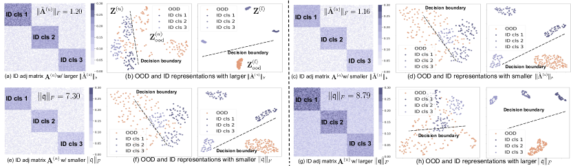
Figure 3: Additional example showcasing the contrast between adjacency matrices and representations w/ (l) and w/o (u) ID labels. (a) The ID adjacency matrix in the unlabeled case $\mathbf{A}^{(u)}$ with a larger $\|\tilde{\mathbf{A}}^{(u)}\|_{F}$ ($B_{1}=0.8,B_{2}=0.1,B_{3}=0.75,B_{4}=0.7$). (b) The contrast of the learned representations in both labeled and unlabeled cases when $\|\tilde{\mathbf{A}}^{(u)}\|_{F}=1.20$. (c) The ID adjacency matrix in the unlabeled case $\mathbf{A}^{(u)}$ with a smaller $\|\tilde{\mathbf{A}}^{(u)}\|_{F}$ ($B_{1}=0.7,B_{2}=0.1,B_{3}=0.65,B_{4}=0.6$). (d) The contrast of the learned representations in both labeled and unlabeled cases when $\|\tilde{\mathbf{A}}^{(u)}\|_{F}=1.16$. Compared with (b) where the difference in the linear probing loss $\mathcal{G}$ is 0.09, the linear probing loss reduces from 0.16 to 0.02. (e) The ID adjacency matrix in the unlabeled case $\mathbf{A}^{(u)}$ with a smaller $\|\mathfrak{q}\|_{F}$ ($B_{1}=0.7,B_{2}=0.1,B_{3}=0.65,B_{4}=0.6$). (f) The contrast of the learned representations in both labeled and unlabeled cases when $\|\mathfrak{q}\|_{F}=7.30$. (g) The ID adjacency matrix in the unlabeled case $\mathbf{A}^{(u)}$ with a larger $\|\mathfrak{q}\|_{F}$ ($B_{1}=0.8,B_{2}=0.2,B_{3}=0.75,B_{4}=0.7$). (h) The contrast of the learned representations in both labeled and unlabeled cases when $\|\mathfrak{q}\|_{F}=8.79$. Compared with (f) where the difference in the linear probing loss $\mathcal{G}$ is 0.14, the linear probing loss reduces from 0.16 to 0.00. The visualization aligns with our theoretical reasoning as shown in Section 4.3.

Appendix H Additional Experimental Details

We provide more training details for both contrastive learning and linear probing. For contrastive training, we use the same data augmentation strategies as SimSiam (Chen & He, 2021). For Cifar10, we set $\phi_{u}=0.5,\phi_{l}=0.25$ with training epoch 200, and we evaluate using features extracted from the layer preceding the projection. For Cifar100, we set $\phi_{u}=3,\phi_{l}=0.0225$ with 200 training epochs and assess based on the projection layer’s features. We use SGD with momentum 0.9 as an optimizer with cosine annealing (lr=0.03), weight decay 5e-4, and batch size 512.

For linear probing, we train a linear layer on the extracted features from the pretrained model by contrastive learning. We use SGD for 50 epochs with momentum 0.9 as an optimizer with a decayed learning rate in epoch 30 by 0.2 (The initial learning rate is 5), and batch size 512.

Appendix I Additional Experimental Results

Results on Cifar10. We present the experimental results on Cifar10 in Table 7, where the effect of the ID labels is similar to the results on Cifar100.

OOD category	OOD dataset	ID labels	FPR95	AUROC	LP error	FPR95	AUROC	LP error
			$\mathbb{P}_{\rm ood}^{\rm test}=\mathbb{P}_{\rm ood}^{\rm LP}$			$\mathbb{P}_{\rm ood}^{\rm test}\neq\mathbb{P}_{\rm ood}^{\rm LP}$
Far OOD	Svhn	-	0.05±0.01	99.98±0.00	0.01±0.00	36.60±2.84	91.71±1.90	0.33±0.11
		+	0.03±0.00	99.98±0.01	0.00±0.00	8.62±1.12	98.43±0.47	0.25±0.19
	Textures	-	0.21±0.03	99.96±0.01	0.01±0.00	10.16±0.72	98.13±2.03	0.52±0.10
		+	0.57±0.06	99.80±0.10	0.01±0.00	13.87±0.82	97.60±1.39	0.58±0.18
	Places365	-	0.36±0.01	99.91±0.00	0.02±0.00	20.19±1.23	96.18±0.28	0.43±0.16
		+	0.68±0.02	99.68±0.06	0.02±0.01	15.83±1.83	97.01±0.96	0.26±0.06
	Lsun-Resize	-	0.68±0.01	99.78±0.18	0.03±0.00	18.21±1.71	96.87±3.28	0.42±0.21
		+	0.56±0.23	99.78±0.10	0.01±0.01	10.83±1.18	97.94±0.23	0.39±0.03
	Lsun-C	-	0.68±0.12	99.80±0.05	0.04±0.02	11.10±1.78	97.93±1.89	0.42±0.07
		+	0.32±0.16	99.65±0.05	0.02±0.02	7.95±1.92	98.44±0.21	0.40±0.19
Near OOD	Cifar100	-	49.88±1.81	89.29±0.99	0.24±0.07	54.76±2.21	86.65±3.04	0.53±0.08
		+	41.56±1.49	92.83±0.73	0.10±0.02	40.04±2.92	92.42±0.18	0.41±0.19

Table 7: OOD detection results w/ and w/o ID labels (Cifar10 as ID). Mean and std are estimated on three different runs. Better results are highlighted in bold. “+,-” denotes the labeled and unlabeled case. “LP error” denotes the error of linear probing.

Results on using post-hoc OOD detection scores. Instead of using linear probing to evaluate the OOD detection performance, we investigate another approach, which directly calculates the $k$-NN score (Sun et al., 2022) on top of the extracted representations for both the ID and OOD data and then computes the OOD detection metrics for comparison. The result is shown in Table 8, where the OOD detection performance is usually better in the labeled case.

OOD category	OOD dataset	ID labels	FPR95	AUROC	FPR95	AUROC
			Cifar10 as ID		Cifar100 as ID
Far OOD	Svhn	-	37.35±3.12	88.08±2.91	27.27±0.88	93.85±2.16
		+	14.97±1.81	97.82±0.96	55.39±4.78	86.31±1.12
	Textures	-	63.91±2.16	78.29±3.06	77.87±1.97	61.68±1.68
		+	44.91±2.90	92.89±0.95	67.19±2.08	81.11±2.89
	Places365	-	65.90±4.02	86.91±3.38	76.52±4.29	70.68±2.90
		+	61.02±2.61	92.65±1.91	64.16±0.72	85.28±1.29
	Lsun-Resize	-	68.91±2.17	85.89±0.90	90.00±1.38	57.91±3.96
		+	56.81±0.61	92.81±1.74	67.40±3.19	85.89±3.77
	Lsun-C	-	26.08±1.48	93.21±0.27	62.57±0.97	75.50±1.98
		+	36.32±2.20	94.97±1.88	57.10±2.93	83.23±2.26
Near OOD	Cifar100/Cifar10	-	71.76±2.49	81.97±0.71	92.10±2.90	58.57±4.86
		+	53.22±2.10	90.94±1.17	84.12±2.26	74.31±0.63

Table 8: OOD detection results measured by post-hoc $k$-NN score w/ and w/o ID labels (Cifar10 and Cifar100 as ID). Mean and std are estimated on three different runs. Better results are highlighted in bold. “+,-” denotes the labeled and unlabeled case and $k$ is set to 25 for all the experiments.

$\|\tilde{\mathbf{A}}_{\mathrm{OI}}^{(u)}\|_{F}$	$\mathcal{G}$	Our bound
60	0.09	0.07
72	0.16	0.12
84	0.21	0.16
96	0.39	0.37
108	0.40	0.34
120	0.61	0.56

Table 9: Numerical results on the bound tightness.

Appendix J Tightness of the Bound

We provide the evidence to verify the tightness of our bound. Specifically, we present numerical results on the illustrative example (Figure 2) to show the proximity between the value of the error difference $\mathcal{G}$ and the bound in our Theorem in Table 9. Specifically, we set a different value of $\|\tilde{\mathbf{A}}_{\mathrm{OI}}^{(u)}\|_{F}$ and observed our lower bound is sufficiently close to the error difference $\mathcal{G}$ (The details of the dataset used are the same as those described in Appendix Section F except for the Frobenius norm of the OOD-ID adjacency matrix).

References

• Ahmed & Courville (2020) Ahmed, F. and Courville, A. Detecting semantic anomalies. In Proceedings of the AAAI Conference on Artificial Intelligence, volume 34, pp.  3154–3162, 2020.
• Argyriou et al. (2005) Argyriou, A., Herbster, M., and Pontil, M. Combining graph laplacians for semi–supervised learning. Advances in Neural Information Processing Systems, 18, 2005.
• Bai et al. (2023) Bai, H., Canal, G., Du, X., Kwon, J., Nowak, R. D., and Li, Y. Feed two birds with one scone: Exploiting wild data for both out-of-distribution generalization and detection. In International Conference on Machine Learning, 2023.
• Baksalary & Puntanen (1992) Baksalary, J. K. and Puntanen, S. An inequality for the trace of matrix product. IEEE transactions on automatic control, 37(2):239–240, 1992.
• Belkin & Niyogi (2003) Belkin, M. and Niyogi, P. Laplacian eigenmaps for dimensionality reduction and data representation. Neural computation, 15(6):1373–1396, 2003.
• Belkin et al. (2006) Belkin, M., Niyogi, P., and Sindhwani, V. Manifold regularization: A geometric framework for learning from labeled and unlabeled examples. Journal of Machine Learning Research, 7(85):2399–2434, 2006.
• Bendale & Boult (2016) Bendale, A. and Boult, T. E. Towards open set deep networks. In Proceedings of the IEEE/CVF Conference on Computer Vision and Pattern Recognition, pp.  1563–1572, 2016.
• Bengio et al. (2003) Bengio, Y., Paiement, J.-f., Vincent, P., Delalleau, O., Roux, N., and Ouimet, M. Out-of-sample extensions for lle, isomap, mds, eigenmaps, and spectral clustering. Advances in neural information processing systems, 16, 2003.
• Bevandić et al. (2018) Bevandić, P., Krešo, I., Oršić, M., and Šegvić, S. Discriminative out-of-distribution detection for semantic segmentation. arXiv preprint arXiv:1808.07703, 2018.
• Blum (2001) Blum, A. Learning form labeled and unlabeled data using graph mincuts. In Proc. 18th International Conference on Machine Learning, 2001, 2001.
• Chandola et al. (2009) Chandola, V., Banerjee, A., and Kumar, V. Anomaly detection: A survey. ACM computing surveys (CSUR), 41(3):1–58, 2009.
• Cheeger (2015) Cheeger, J. A lower bound for the smallest eigenvalue of the laplacian. In Problems in analysis, pp.  195–200. Princeton University Press, 2015.
• Chen et al. (2020) Chen, T., Kornblith, S., Norouzi, M., and Hinton, G. A simple framework for contrastive learning of visual representations. In International conference on machine learning, pp.  1597–1607. PMLR, 2020.
• Chen & He (2021) Chen, X. and He, K. Exploring simple siamese representation learning. In Proceedings of the IEEE/CVF conference on computer vision and pattern recognition, pp.  15750–15758, 2021.
• Chung (1997) Chung, F. R. Spectral graph theory, volume 92. American Mathematical Soc., 1997.
• Cimpoi et al. (2014) Cimpoi, M., Maji, S., Kokkinos, I., Mohamed, S., and Vedaldi, A. Describing textures in the wild. In Proceedings of the IEEE/CVF Conference on Computer Vision and Pattern Recognition, pp.  3606–3613, 2014.
• Djurisic et al. (2023) Djurisic, A., Bozanic, N., Ashok, A., and Liu, R. Extremely simple activation shaping for out-of-distribution detection. In International Conference on Learning Representations, 2023.
• Du et al. (2022a) Du, X., Gozum, G., Ming, Y., and Li, Y. Siren: Shaping representations for detecting out-of-distribution objects. In Advances in Neural Information Processing Systems, 2022a.
• Du et al. (2022b) Du, X., Wang, X., Gozum, G., and Li, Y. Unknown-aware object detection: Learning what you don’t know from videos in the wild. In Proceedings of the IEEE/CVF Conference on Computer Vision and Pattern Recognition, 2022b.
• Du et al. (2022c) Du, X., Wang, Z., Cai, M., and Li, Y. Vos: Learning what you don’t know by virtual outlier synthesis. In Proceedings of the International Conference on Learning Representations, 2022c.
• Du et al. (2023) Du, X., Sun, Y., Zhu, X., and Li, Y. Dream the impossible: Outlier imagination with diffusion models. In Advances in Neural Information Processing Systems, 2023.
• Du et al. (2024) Du, X., Fang, Z., Diakonikolas, I., and Li, Y. How does unlabeled data provably help out-of-distribution detection? In Proceedings of the International Conference on Learning Representations, 2024.
• Eckart & Young (1936) Eckart, C. and Young, G. The approximation of one matrix by another of lower rank. Psychometrika, 1(3):211–218, 1936.
• Fang et al. (1994) Fang, Y., Loparo, K., and Feng, X. Inequalities for the trace of matrix product. IEEE Transactions on Automatic Control, 39(12):2489–2490, 1994.
• Fang et al. (2022) Fang, Z., Li, Y., Lu, J., Dong, J., Han, B., and Liu, F. Is out-of-distribution detection learnable? In Advances in Neural Information Processing Systems, 2022.
• Fort et al. (2021) Fort, S., Ren, J., and Lakshminarayanan, B. Exploring the limits of out-of-distribution detection. Advances in Neural Information Processing Systems, 34:7068–7081, 2021.
• Gal & Ghahramani (2016) Gal, Y. and Ghahramani, Z. Dropout as a bayesian approximation: Representing model uncertainty in deep learning. In Proceedings of the International Conference on Machine Learning, pp.  1050–1059, 2016.
• Galil et al. (2023) Galil, I., Dabbah, M., and El-Yaniv, R. A framework for benchmarking class-out-of-distribution detection and its application to imagenet. In International Conference on Learning Representations, 2023.
• Geifman & El-Yaniv (2019) Geifman, Y. and El-Yaniv, R. Selectivenet: A deep neural network with an integrated reject option. In Proceedings of the International Conference on Machine Learning, pp.  2151–2159, 2019.
• Ghosal et al. (2024) Ghosal, S. S., Sun, Y., and Li, Y. How to overcome curse-of-dimensionality for ood detection? In Proceedings of the AAAI Conference on Artificial Intelligence, 2024.
• Greenbaum et al. (2020) Greenbaum, A., Li, R.-c., and Overton, M. L. First-order perturbation theory for eigenvalues and eigenvectors. SIAM review, 62(2):463–482, 2020.
• Han et al. (2022) Han, S., Hu, X., Huang, H., Jiang, M., and Zhao, Y. Adbench: Anomaly detection benchmark. Advances in Neural Information Processing Systems, 35:32142–32159, 2022.
• HaoChen et al. (2021) HaoChen, J. Z., Wei, C., Gaidon, A., and Ma, T. Provable guarantees for self-supervised deep learning with spectral contrastive loss. Advances in Neural Information Processing Systems, 34:5000–5011, 2021.
• HaoChen et al. (2022) HaoChen, J. Z., Wei, C., Kumar, A., and Ma, T. Beyond separability: Analyzing the linear transferability of contrastive representations to related subpopulations. Advances in Neural Information Processing Systems, 2022.
• He et al. (2016) He, K., Zhang, X., Ren, S., and Sun, J. Deep residual learning for image recognition. In Proceedings of the IEEE conference on computer vision and pattern recognition, pp.  770–778, 2016.
• He et al. (2023) He, R., Li, R., Han, Z., Yang, X., and Yin, Y. Topological structure learning for weakly-supervised out-of-distribution detection. In Proceedings of the 31st ACM International Conference on Multimedia, pp.  4858–4866, 2023.
• Hein et al. (2019) Hein, M., Andriushchenko, M., and Bitterwolf, J. Why relu networks yield high-confidence predictions far away from the training data and how to mitigate the problem. In Proceedings of the IEEE/CVF Conference on Computer Vision and Pattern Recognition, pp.  41–50, 2019.
• Hendrycks & Gimpel (2017) Hendrycks, D. and Gimpel, K. A baseline for detecting misclassified and out-of-distribution examples in neural networks. Proceedings of the International Conference on Learning Representations, 2017.
• Hendrycks et al. (2019) Hendrycks, D., Mazeika, M., and Dietterich, T. Deep anomaly detection with outlier exposure. In Proceedings of the International Conference on Learning Representations, 2019.
• Huang et al. (2021) Huang, R., Geng, A., and Li, Y. On the importance of gradients for detecting distributional shifts in the wild. In Advances in Neural Information Processing Systems, 2021.
• Jansen et al. (2015) Jansen, A., Sell, G., and Lyzinski, V. Scalable out-of-sample extension of graph embeddings using deep neural networks. arXiv preprint arXiv:1508.04422, 2015.
• Jeong & Kim (2020) Jeong, T. and Kim, H. Ood-maml: Meta-learning for few-shot out-of-distribution detection and classification. Advances in Neural Information Processing Systems, 33:3907–3916, 2020.
• Kannan et al. (2004) Kannan, R., Vempala, S., and Vetta, A. On clusterings: Good, bad and spectral. Journal of the ACM (JACM), 51(3):497–515, 2004.
• Katz-Samuels et al. (2022) Katz-Samuels, J., Nakhleh, J., Nowak, R., and Li, Y. Training ood detectors in their natural habitats. In International Conference on Machine Learning, 2022.
• Kristiadi et al. (2020) Kristiadi, A., Hein, M., and Hennig, P. Being bayesian, even just a bit, fixes overconfidence in relu networks. In International conference on machine learning, pp.  5436–5446, 2020.
• Krizhevsky et al. (2009) Krizhevsky, A., Hinton, G., et al. Learning multiple layers of features from tiny images. 2009.
• Lakshminarayanan et al. (2017) Lakshminarayanan, B., Pritzel, A., and Blundell, C. Simple and scalable predictive uncertainty estimation using deep ensembles. In Advances in Neural Information Processing Systems, volume 30, pp.  6402–6413, 2017.
• Lee et al. (2014) Lee, J. R., Gharan, S. O., and Trevisan, L. Multiway spectral partitioning and higher-order cheeger inequalities. Journal of the ACM (JACM), 61(6):1–30, 2014.
• Lee et al. (2018a) Lee, K., Lee, H., Lee, K., and Shin, J. Training confidence-calibrated classifiers for detecting out-of-distribution samples. In Proceedings of the International Conference on Learning Representations, 2018a.
• Lee et al. (2018b) Lee, K., Lee, K., Lee, H., and Shin, J. A simple unified framework for detecting out-of-distribution samples and adversarial attacks. Advances in Neural Information Processing Systems, 31, 2018b.
• Levin et al. (2018) Levin, K., Roosta, F., Mahoney, M., and Priebe, C. Out-of-sample extension of graph adjacency spectral embedding. In International Conference on Machine Learning, pp.  2975–2984. PMLR, 2018.
• Liang et al. (2018) Liang, S., Li, Y., and Srikant, R. Enhancing the reliability of out-of-distribution image detection in neural networks. In Proceedings of the International Conference on Learning Representations, 2018.
• Liu et al. (2020a) Liu, J., Lin, Z., Padhy, S., Tran, D., Bedrax Weiss, T., and Lakshminarayanan, B. Simple and principled uncertainty estimation with deterministic deep learning via distance awareness. Advances in Neural Information Processing Systems, 33:7498–7512, 2020a.
• Liu et al. (2020b) Liu, W., Wang, X., Owens, J., and Li, Y. Energy-based out-of-distribution detection. Advances in Neural Information Processing Systems, 33:21464–21475, 2020b.
• Maddox et al. (2019) Maddox, W. J., Izmailov, P., Garipov, T., Vetrov, D. P., and Wilson, A. G. A simple baseline for bayesian uncertainty in deep learning. Advances in Neural Information Processing Systems, 32:13153–13164, 2019.
• Malinin & Gales (2018) Malinin, A. and Gales, M. Predictive uncertainty estimation via prior networks. Advances in Neural Information Processing Systems, 31, 2018.
• Malinin & Gales (2019) Malinin, A. and Gales, M. Reverse kl-divergence training of prior networks: Improved uncertainty and adversarial robustness. In Advances in Neural Information Processing Systems, 2019.
• McSherry (2001) McSherry, F. Spectral partitioning of random graphs. In Proceedings 42nd IEEE Symposium on Foundations of Computer Science, pp.  529–537. IEEE, 2001.
• Meinke & Hein (2020) Meinke, A. and Hein, M. Towards neural networks that provably know when they don’t know. In Proceedings of the International Conference on Learning Representations, 2020.
• Ming & Li (2023) Ming, Y. and Li, Y. How does fine-tuning impact out-of-distribution detection for vision-language models? International Journal of Computer Vision, 2023.
• Ming et al. (2022a) Ming, Y., Cai, Z., Gu, J., Sun, Y., Li, W., and Li, Y. Delving into out-of-distribution detection with vision-language representations. In Advances in Neural Information Processing Systems, 2022a.
• Ming et al. (2022b) Ming, Y., Fan, Y., and Li, Y. POEM: out-of-distribution detection with posterior sampling. In Proceedings of the International Conference on Machine Learning, pp.  15650–15665, 2022b.
• Ming et al. (2022c) Ming, Y., Yin, H., and Li, Y. On the impact of spurious correlation for out-of-distribution detection. In Proceedings of the AAAI Conference on Artificial Intelligence, 2022c.
• Ming et al. (2023) Ming, Y., Sun, Y., Dia, O., and Li, Y. How to exploit hyperspherical embeddings for out-of-distribution detection? In Proceedings of the International Conference on Learning Representations, 2023.
• Morteza & Li (2022) Morteza, P. and Li, Y. Provable guarantees for understanding out-of-distribution detection. In Proceedings of the AAAI Conference on Artificial Intelligence, volume 36, pp.  7831–7840, 2022.
• Narasimhan et al. (2023) Narasimhan, H., Menon, A. K., Jitkrittum, W., and Kumar, S. Learning to reject meets ood detection: Are all abstentions created equal? arXiv preprint arXiv:2301.12386, 2023.
• Netzer et al. (2011) Netzer, Y., Wang, T., Coates, A., Bissacco, A., Wu, B., and Ng, A. Y. Reading digits in natural images with unsupervised feature learning. 2011.
• Ng et al. (2001) Ng, A., Jordan, M., and Weiss, Y. On spectral clustering: Analysis and an algorithm. Advances in neural information processing systems, 14, 2001.
• Park et al. (2023) Park, S., Mok, J., Jung, D., Lee, S., and Yoon, S. On the powerfulness of textual outlier exposure for visual ood detection. arXiv preprint arXiv:2310.16492, 2023.
• Quispe et al. (2016) Quispe, A. M., Petitjean, C., and Heutte, L. Extreme learning machine for out-of-sample extension in laplacian eigenmaps. Pattern Recognition Letters, 74:68–73, 2016.
• Ren et al. (2021) Ren, J., Fort, S., Liu, J., Roy, A. G., Padhy, S., and Lakshminarayanan, B. A simple fix to mahalanobis distance for improving near-ood detection. CoRR, abs/2106.09022, 2021.
• Ren et al. (2023) Ren, J., Luo, J., Zhao, Y., Krishna, K., Saleh, M., Lakshminarayanan, B., and Liu, P. J. Out-of-distribution detection and selective generation for conditional language models. In International Conference on Learning Representations, 2023.
• Sehwag et al. (2021a) Sehwag, V., Chiang, M., and Mittal, P. Ssd: A unified framework for self-supervised outlier detection. In International Conference on Learning Representations, 2021a.
• Sehwag et al. (2021b) Sehwag, V., Chiang, M., and Mittal, P. Ssd: A unified framework for self-supervised outlier detection. In Proceedings of the International Conference on Learning Representations, 2021b.
• Shaham et al. (2018) Shaham, U., Stanton, K., Li, H., Nadler, B., Basri, R., and Kluger, Y. Spectralnet: Spectral clustering using deep neural networks. In 6th International Conference on Learning Representations, ICLR 2018, 2018.
• Shen et al. (2022) Shen, K., Jones, R. M., Kumar, A., Xie, S. M., HaoChen, J. Z., Ma, T., and Liang, P. Connect, not collapse: Explaining contrastive learning for unsupervised domain adaptation. In International Conference on Machine Learning, pp.  19847–19878, 2022.
• Shi & Malik (2000) Shi, J. and Malik, J. Normalized cuts and image segmentation. IEEE Transactions on pattern analysis and machine intelligence, 22(8):888–905, 2000.
• Sun et al. (2022) Sun, Y., Ming, Y., Zhu, X., and Li, Y. Out-of-distribution detection with deep nearest neighbors. In Proceedings of the International Conference on Machine Learning, pp.  20827–20840, 2022.
• Sun et al. (2023a) Sun, Y., Shi, Z., and Li, Y. A graph-theoretic framework for understanding open-world representation learning. In Advances in Neural Information Processing Systems, 2023a.
• Sun et al. (2023b) Sun, Y., Shi, Z., Liang, Y., and Li, Y. When and how does known class help discover unknown ones? provable understandings through spectral analysis. In International Conference on Machine Learning, 2023b.
• Sussman et al. (2012) Sussman, D. L., Tang, M., Fishkind, D. E., and Priebe, C. E. A consistent adjacency spectral embedding for stochastic blockmodel graphs. Journal of the American Statistical Association, 107(499):1119–1128, 2012.
• Tack et al. (2020) Tack, J., Mo, S., Jeong, J., and Shin, J. Csi: Novelty detection via contrastive learning on distributionally shifted instances. In Advances in Neural Information Processing Systems, 2020.
• Tang et al. (2013) Tang, M., Sussman, D. L., and Priebe, C. E. Universally consistent vertex classification for latent positions graphs. The Annals of Statistics, 41(3):1406–1430, 2013.
• Tao et al. (2023) Tao, L., Du, X., Zhu, X., and Li, Y. Non-parametric outlier synthesis. In Proceedings of the International Conference on Learning Representations, 2023.
• Trosset & Priebe (2008) Trosset, M. W. and Priebe, C. E. The out-of-sample problem for classical multidimensional scaling. Computational statistics & data analysis, 52(10):4635–4642, 2008.
• Uppaal et al. (2023) Uppaal, R., Hu, J., and Li, Y. Is fine-tuning needed? pre-trained language models are near perfect for out-of-domain detection. In Annual Meeting of the Association for Computational Linguistics, 2023.
• van Amersfoort et al. (2020) van Amersfoort, J., Smith, L., Teh, Y. W., and Gal, Y. Uncertainty estimation using a single deep deterministic neural network. In Proceedings of the International Conference on Machine Learning, pp.  9690–9700, 2020.
• Von Luxburg (2007) Von Luxburg, U. A tutorial on spectral clustering. Statistics and computing, 17(4):395–416, 2007.
• Wang et al. (2021) Wang, H., Liu, W., Bocchieri, A., and Li, Y. Can multi-label classification networks know what they don’t know? Proceedings of the Advances in Neural Information Processing Systems, 2021.
• Wang et al. (2022a) Wang, Q., Liu, F., Zhang, Y., Zhang, J., Gong, C., Liu, T., and Han, B. Watermarking for out-of-distribution detection. Advances in Neural Information Processing Systems, 35:15545–15557, 2022a.
• Wang et al. (2023a) Wang, Q., Fang, Z., Zhang, Y., Liu, F., Li, Y., and Han, B. Learning to augment distributions for out-of-distribution detection. Advances in Neural Information Processing Systems, 2023a.
• Wang et al. (2023b) Wang, Q., Ye, J., Liu, F., Dai, Q., Kalander, M., Liu, T., HAO, J., and Han, B. Out-of-distribution detection with implicit outlier transformation. In International Conference on Learning Representations, 2023b.
• Wang et al. (2022b) Wang, Y., Zou, J., Lin, J., Ling, Q., Pan, Y., Yao, T., and Mei, T. Out-of-distribution detection via conditional kernel independence model. In Advances in Neural Information Processing Systems, 2022b.
• Wei et al. (2022) Wei, H., Xie, R., Cheng, H., Feng, L., An, B., and Li, Y. Mitigating neural network overconfidence with logit normalization. In Proceedings of the International Conference on Machine Learning, pp.  23631–23644, 2022.
• Wen et al. (2020) Wen, Y., Tran, D., and Ba, J. Batchensemble: an alternative approach to efficient ensemble and lifelong learning. In International Conference on Learning Representations, 2020.
• Wu et al. (2023) Wu, Q., Chen, Y., Yang, C., and Yan, J. Energy-based out-of-distribution detection for graph neural networks. In International Conference on Learning Representations, 2023.
• Yang et al. (2021a) Yang, J., Wang, H., Feng, L., Yan, X., Zheng, H., Zhang, W., and Liu, Z. Semantically coherent out-of-distribution detection. In Proceedings of the International Conference on Computer Vision, pp.  8281–8289, 2021a.
• Yang et al. (2021b) Yang, J., Zhou, K., Li, Y., and Liu, Z. Generalized out-of-distribution detection: A survey. arXiv preprint arXiv:2110.11334, 2021b.
• Yang et al. (2022) Yang, J., Wang, P., Zou, D., Zhou, Z., Ding, K., PENG, W., Wang, H., Chen, G., Li, B., Sun, Y., Du, X., Zhou, K., Zhang, W., Hendrycks, D., Li, Y., and Liu, Z. OpenOOD: Benchmarking generalized out-of-distribution detection. In Advances on Neural Information Processing Systems, Datasets and Benchmarks Track, 2022.
• Yang et al. (2023) Yang, P., Liang, J., Cao, J., and He, R. Auto: Adaptive outlier optimization for online test-time ood detection. arXiv preprint arXiv:2303.12267, 2023.
• Yu et al. (2015) Yu, F., Seff, A., Zhang, Y., Song, S., Funkhouser, T., and Xiao, J. Lsun: Construction of a large-scale image dataset using deep learning with humans in the loop. arXiv preprint arXiv:1506.03365, 2015.
• Zhang et al. (2023) Zhang, J., Yang, J., Wang, P., Wang, H., Lin, Y., Zhang, H., Sun, Y., Du, X., Zhou, K., Zhang, W., et al. Openood v1. 5: Enhanced benchmark for out-of-distribution detection. arXiv preprint arXiv:2306.09301, 2023.
• Zheng et al. (2023) Zheng, H., Wang, Q., Fang, Z., Xia, X., Liu, F., Liu, T., and Han, B. Out-of-distribution detection learning with unreliable out-of-distribution sources. arXiv preprint arXiv:2311.03236, 2023.
• Zhou et al. (2017) Zhou, B., Lapedriza, A., Khosla, A., Oliva, A., and Torralba, A. Places: A 10 million image database for scene recognition. IEEE transactions on pattern analysis and machine intelligence, 40(6):1452–1464, 2017.
• Zhou et al. (2021) Zhou, Z., Guo, L.-Z., Cheng, Z., Li, Y.-F., and Pu, S. STEP: Out-of-distribution detection in the presence of limited in-distribution labeled data. In Advances in Neural Information Processing Systems, 2021.
• Zhu et al. (2023a) Zhu, J., Li, H., Yao, J., Liu, T., Xu, J., and Han, B. Unleashing mask: Explore the intrinsic out-of-distribution detection capability. arXiv preprint arXiv:2306.03715, 2023a.
• Zhu et al. (2023b) Zhu, J., Yu, G., Yao, J., Liu, T., Niu, G., Sugiyama, M., and Han, B. Diversified outlier exposure for out-of-distribution detection via informative extrapolation. arXiv preprint arXiv:2310.13923, 2023b.
• Zhu et al. (2003) Zhu, X., Ghahramani, Z., and Lafferty, J. D. Semi-supervised learning using gaussian fields and harmonic functions. In Proceedings of the 20th International conference on Machine learning (ICML-03), pp.  912–919, 2003.
• Zhu et al. (2022) Zhu, Y., Chen, Y., Xie, C., Li, X., Zhang, R., Xue’, H., Tian, X., bolun zheng, and Chen, Y. Boosting out-of-distribution detection with typical features. In Advances in Neural Information Processing Systems, 2022.