A Theoretical Understanding of Self-Correction through In-context Alignment

Abstract

Going beyond mimicking limited human experiences, recent studies show initial evidence that, like humans, large language models (LLMs) are capable of improving their abilities purely by self-correction, i.e., correcting previous responses through self-examination, in certain circumstances. Nevertheless, little is known about how such capabilities arise. In this work, based on a simplified setup akin to an alignment task, we theoretically analyze self-correction from an in-context learning perspective, showing that when LLMs give relatively accurate self-examinations as rewards, they are capable of refining responses in an in-context way. Notably, going beyond previous theories on over-simplified linear transformers, our theoretical construction underpins the roles of several key designs of realistic transformers for self-correction: softmax attention, multi-head attention, and the MLP block. We validate these findings extensively on synthetic datasets. Inspired by these findings, we also illustrate novel applications of self-correction, such as defending against LLM jailbreaks, where a simple self-correction step does make a large difference. We believe that these findings will inspire further research on understanding, exploiting, and enhancing self-correction for building better foundation models.

1 Introduction

Who among people is without fault? Making mistakes and being able to correct them is the greatest goodness. — Zuo Zhuan ($\sim$400 BC), Translated by ChatGPT

The capacity for self-correction, traditionally viewed as a distinctive human trait, is increasingly being explored within the realm of artificial intelligence, particularly in Large Language Models (LLMs). Recent studies have sparked optimism about LLMs’ self-correction capabilities for enhancing reasoning [49, 65, 75], planning [79], and alignment [6, 23]. Although some find that self-correction may lead to worse performance without external feedbacks [30, 69], more recent evidence shows that with careful designs of instructions on the self-criticizing process, self-correction can yield considerable benefits on various tasks [40, 85, 44, 34, 36, 68].

Driven by these intruiging empirical findings, we want to establish a principled understanding of how the self-correction ability emerges in LLMs. A particular difficulty is to formulate the multifaceted self-correction designs to be amenable to theoretical analysis. We notice that existing self-correction methods admit a general abstraction: generation, critics, regeneration, and further critics, continuing until the final refined output. This self-correction path can be understood as a particular form of context that provides feedback for refining the prediction on the fly. Different from standard (query, response) context examples akin to supervised learning, self-correction examples can be formulated in a triplet form (query, response, reward) that is akin to LLM alignment with both good and bad samples indicated by their rewards [53, 8, 61, 61, 66]. This observation motivates us to formulate self-correction as a form of in-context alignment (ICA), where LLMs are provided with a context of self-correction steps and the goal is to refine the final outputs to have higher rewards.

Through this perspective, we prove that in a simplified setup, a standard multi-layer transformer can utilize self-correction samples to generate responses of higher rewards. Specifically, we prove the existence of model weights such that a transformer can optimize common ranking-based alignment objectives by performing gradient descent in-context, which includes the Bradley-Terry model [10] and the Plackett-Luce model [58] that are de facto choices for LLM alignment (used in RLHF [53] and DPO [61]). As far as we know, this is the first theoretical analysis showing that LLMs can improve alignment in-context, providing a solid foundation for understanding self-correction. Our theory accommodates different kinds of self-correction methods, because the critics of responses can come from humans [53], external verifiers [14], or LLMs themselves [85, 40]. The analysis further reveals that LLMs’ self-correction performance relies crucially on the quality of critics, which agrees well with recent empirical findings [44, 15, 68]. Intriguingly, within this analysis, we nail down the roles of realistic transformer designs – multi-head softmax attention, feed-forward network, and stacked blocks – for alignment, providing concrete theoretical insights for designing robust LLMs. This contrasts with previous in-context learning theories that focus on linear attention in the context of linear regression, deviating from practice [73, 82, 2].

At last, we validate our theoretical explanations through both synthetic and real-world experiments. Extensive synthetic datasets show that transformers can indeed learn from noisy outputs with the help of relatively accurate critics. We validate that real-world transformer modules do matter for in-context alignment, and the results align surprisingly well with our theory. Driven by these theoretical insights, we explore two real-world scenarios where we hypothesize that aligned LLMs can provide relatively accurate self-critics: alleviating social bias and defending against jailbreak attacks. We show that with a simple generation-critic-regeneration process (we call Checking-as-Context) and no external feedback, intrinsic self-correction can alleviate social bias on Vicuna-7b and Llama2-7b-chat, and exhibits a strong correlation between self-checking accuracy and final performance again. With the same strategy, we find that self-correction can reduce the attack success rate by a large margin (e.g., $95\%\to 2\%$) against multiple types of jailbreak attacks. These evidences show that LLMs are indeed capable of improving alignment by self-correction alone, which not only validates our theory, but also provide insights for future designs and applications of self-correction.

2 Formulation

In this section, we introduce self-correction and formulate it as a general in-context alignment process, and then introduce the setup for theoretical analysis.

2.1 Self-correction as In-context Alignment

ICL. In-context learning (ICL) is known as an emergent ability of LLMs to learn from a few demonstrations without finetuning [47]. Specifically, an LLM can directly predict the desirable response to the test query $x_{test}$ with $N$ pairwise training examples $\{(x_{i},y_{i})\}_{i=1}^{n}$ as the context:

$$\hat{y}_{test}=\operatorname{LLM}([x_{1},y_{1},\dots,x_{n},y_{n},x_{test}]).$$ (1)

Despite its effectiveness, ICL requires the knowledge of desirable responses $y_{i}$ to construct the training examples. For instance, Wei et al. [76] use human-selected safe query-response pairs for in-context defense of jailbreaks. For queries that are vague or require domain expertise (e.g., math, science, and open-end discussions), desirable responses can be hard to collect or formulate.

Self-correction. As a further step to eliminate human efforts, self-correction relies on LLMs to correct the mistakes in the initial generation. In self-correction, we first generate an initial response $y_{1}$ to the query $x$, and then obtain a critic on the response, denoted as a reward $r_{1}$. The critic can be either generated by LLMs themselves through carefully designed prompting [36, 40], or by external verifiers such as code intepreters [62]. Afterwards, the LLM is then instructed to generate a refined response $y_{2}$ taking the initial response $y_{1}$ and its critic $r_{1}$ as the input context. This process can be repeated multiple times for iterative refinements of the response. After $N$ steps, we take the final response $y_{N}$ as the final output. For simplicity, we assume that these steps share the same query $x$, and the extension to multiple queries is discussed in Appendix F.1.

In-context Alignment (ICA). The self-correction process described above can be formalized as an in-context learning task with triplet examples $\{(x,y_{i},r_{i})\}$, where $x$ is the (shared) query, $y_{i}$ is the response, and $r_{i}$ is the critic at the $i$-th step. Note that the same data format is also adopted in LLM alignment tasks, where LLMs are trained to follow human intention with human/AI-generated preference data [53, 8, 61, 66]. In this way, we formulate self-correction as an in-context way to solve an alignment task, which we call in-context alignment (ICA). Here, the concept of alignment is inclusive and not limited to standard alignment tasks. Any objective that works with the triplet preference data can fit into our framework. Also, we do not assume that the rewards $r_{i}$ are always accurate, and the quality of the rewards will be shown to have a critical influence on self-correction.

2.2 Theoretical Setup

Since real-world LLMs on language tasks are too complex for a rigorous analysis, recent studies on ICL theory rely on synethetic simple tasks to examine LLM capabilities [26, 73, 82, 2]. Existing results are mostly established in the supervised setting, particularly for linear regression, due to its simplicity and alignment with linear attention. However, it is yet unknown whether transformers are capable of learning alignment tasks using preference data in-context. In this section, we introduce a simplified setup for in-context alignment. For the ease of analysis, we still study a linear regresion task, where a smaller MSE loss gets higher reward. However, what makes things harder is that the models are not provided with groundtruth targets as the context, but only (potentially false) responses $y_{i}$ and their rewards $r_{i}$. To solve this task, the model has to learn the ability to compare the rewards of different samples and prioritize those with higher rewards – a critical ability that is key to self-correction and alignment, but has not been studied in previous theories.

2.2.1 Alignment Task

We begin by formalizing a general alignment task with triplet examples. Consider a training dataset $D=\{(x,y_{i},r_{i})\}_{i=1}^{n-1}$ composed of a common query $x\in{\mathbb{R}}^{n_{x}}$ (assume $\|x\|^{2}=1$ for simplicity), multiple responses $y_{i}\in{\mathbb{R}}^{n_{y}}$ and rewards $r_{i}\in{\mathbb{R}}$. Following the setup of Von Oswald et al. [73], we also consider a linear regression task where the groundtruth function is $f(x)=W^{*}x$ for some $W^{*}\in{\mathbb{R}}^{n_{y}\times n_{x}}$. However, in our tasks, the responses $y_{i}$ can be quite noisy (e.g., random), and the quality of this response is indicated by its reward value. Therefore, the transformers have to rank the responses based on their rewards and adjust their outputs accordingly. Meanwhile, the rewards coming from humans, external verifiers, or LLMs can also contain noise, which reflect the critic quality. The goal is to output a response $y_{N}$ that has a smaller square error, i.e., higher rewards. There are two approaches to solve this problem, one is through the in-context alignment with a transformer-based LLM, and one is through learning a parameterized alignment model. We describe these methods formally below, and establish their inherent connections in the next section.

2.2.2 Transformer Model

The transformer model [71] is the de facto choice for building LLMs. It is a composition of multiple transformer blocks. Each block consists of two modules: MHSA and FFN. Normalization layers are omitted for simplicity.

MHSA. A multi-head self-attention (MHSA) layer updates a set of tokens $\{e_{1},\dots,e_{N}\}$ by

$$e_{j} \leftarrow e_{j}+\operatorname{SA}_{\theta}\left(j,\left\{e_{1},\ldots,e_{N}\right\}\right)=e_{j}+\sum_{h}P_{h}V_{h}\operatorname{softmax}\left(K_{h}^{\top}q_{h,j}\right),$$ (2)

with $P_{h},V_{h},K_{h}$ the projection, value and key matrices, respectively, and $q_{h,j}$ the query, all for the $h$-th head (bias terms omitted). The columns of the value $V_{h}=\left[v_{h,1},\ldots,v_{h,N}\right]$ and key $K_{h}=\left[k_{h,1},\ldots,k_{h,N}\right]$ matrices consist of vectors $v_{h,i}=W_{h,V}e_{i}$ and $k_{h,i}=W_{h,K}e_{i}$; likewise, the query is produced by linearly projecting the tokens, $q_{h,j}=W_{h,Q}e_{j}$. The parameters $\theta=\left\{P_{h},W_{h,V},W_{h,K},W_{h,Q}\right\}_{h}$ of a SA layer consist of all the projection matrices of all heads. We omit causal masking in the main paper for simplicity; see Appendix F.2 for an extension.

FFN. Following self-attention, a feed-forward network (FFN) transforms each token individually with two shared linear transformations and a ReLU activation in between:

$$e_{j}\leftarrow e_{j}+\operatorname{FFN}_{\phi}(e_{j}),$$ (3)

$$= e_{j}+W_{2}\max(0,W_{1}x+b_{1})+b_{2}.$$

Here, $W_{1},W_{2}$ are weight matrices and $b_{1},b_{2}$ are bias vectors. Collectively, $\phi=(W_{1},b_{1},W_{2},b_{2})$ denotes all FNN parameters. Both SA and FFN have residual connections.

Context Tokens. For simplicity, we assume that LLMs take a concatenated input $e_{i}=[x_{i},y_{i},r_{i}]$ for each example. For the last test example, to align with the same input format, we model it as $e_{N}=[x,y_{N},r_{N}]$, where we use a “dummy” response $y_{N}=W_{0}x_{N}$ (i.e., the initial guess of LLMs with weights $W_{0}$ (Section 2.2.3)) as an initialization for the final output, and its “dummy” reward $r_{N}$ is assumed to have the lowest reward among the input examples. In total, we have $N$ tokens $\{e_{i}=[x,y_{i},r_{i}]\}_{i=1}^{N}$ as the contextual input to the transformer.

2.2.3 Alignment Model

A common way to solve alignment tasks is to learn a parameterized alignment model that models preferences through a ranking objective over multiple candidates [10, 58, 48, 61]. We use $y_{i}\succ y_{j}$ to denote the event that the response $y_{i}$ is preferable over $y_{j}$. Let $\tau\colon[N]\mapsto[N]$ be the permutation function that denotes the ranking of all responses according to the reward scores, i.e., $r_{\tau(1)}>\cdots>r_{\tau(N)}$. The ranking $\tau$ implies that for any $N\geq i>j\geq 1$, we have $y_{\tau(i)}\succ y_{\tau(j)}$. A common objective for $N$-ary comparison is the Plackett-Luce (PL) model [58, 48, 61] that stipulates

$$P_{\rm PL}\left(\tau\mid x,\{y_{i}\}\right)=\prod_{i=1}^{N}\frac{\exp\left(r(x,y_{\tau(i)})\right)}{\sum_{j=i}^{N}\exp\left(r(x,y_{\tau(j)})\right)},$$ (4)

where $r$ denotes the reward function. Since we consider a linear regression task (Section 2.2.1), we use the negative square error as the reward function (higher is better): $r(x,y)=-\|Wx-y\|^{2}.$ The corresponding PL model is

$$P_{\rm PL}\left(\tau\right)=\prod_{i=1}^{N}\frac{\exp\left(-\|Wx-y_{\tau(i)}\|^{2}\right)}{\sum_{j=i}^{N}\exp\left(-\|Wx-y_{\tau(j)}\|^{2}\right)}.$$ (5)

Relationship to Bradley-Terry model. The Plackett-Luce model is an $N$-ary generalization of the Bradley-Terry model [10] used for pariwise preferences. In particular, with $N=2$, the PL model (Eq. (5)) reduces to the Bradley-Terry model with least-squares reward:

$$P_{\rm BT}\left(y_{1}\succ y_{2}\right)=\frac{\exp\left(-\|Wx-y_{1}\|^{2}\right)}{\sum_{j=1}^{2}\exp\left(-\|Wx-y_{i}\|^{2}\right)}.$$ (6)

Previous work [66] shows that the $N$-ary PL model outperforms the binary BT model for alignment.

Relationship to InfoNCE. We also notice that the InfoNCE loss that is widely used for contrastive learning [52, 13, 60] can be seen as a special case of the PL model when only considering its first term ($i=1$). In this case, only $y_{1}$ is the positive sample and $y_{2},\dots,y_{N}$ are negative samples, which corresponds to a special ranking $r_{\tau(1)}>r_{\tau(2)}=\cdots=r_{\tau(N)}$. Therefore, the analysis in our framework can be used to explain in-context contrastive learning [18].

3 Main Results

In this section, we present the main result of this work, which, to the best of our knowledge, is the first to show that a realistic transformer (with stacked multi-head softmax attention and feed-forward networks) can implement the gradient descent of common alignment objectives with in-context triplets. Notably, our analysis reveals the individual roles of these core designs of realistic transformers for in-context alignment (and self-correction), which may help future designs of LLM backbones as well.

3.1 A Simple Case: Bradley-Terry Model with $N=2$

To highlight the key ideas without technical nuances, we start with $N=2$, the Bradley-Terry (BT) model (Eq. (6)). Assume w.l.o.g. that $y_{1}\succ y_{2}$ with scores $r_{1}>r_{2}$, the BT model is ${\mathcal{L}}_{\rm BT}(W;x,y_{1},y_{2})=-\log P_{\rm BT}\left(y_{1}\succ y_{2}\mid x\right)=\|Wx-{y_{1}}\|^{2}+\log\sum_{j=1}^{2}\exp\left(-\|Wx-{y_{j}}\|^{2}\right).$

Proposition 3.1.

One can realize the gradient descent for BT,

$$W^{\prime}=W+\Delta W=W-\eta\nabla_{W}{\mathcal{L}}_{\rm BT}(W;x,y_{1},y_{2}),$$

by updating each $y_{i}$ with

$$y^{\prime}_{i}= \ y_{i}-\Delta Wx=\underbrace{y_{i}}_{\text{(1)}}-\underbrace{2\eta y_{1}}_{\text{(2)}}\underbrace{+2\eta\sum\nolimits_{j=1}^{2}\beta_{j}y_{j}}_{\text{(3)}},$$ (7)

where $\beta_{j}=\mathrm{softmax}(-\|Wx-y_{j}\|^{2})$. Specifically, ${\mathcal{L}}_{\rm BT}(W^{\prime};x,y_{1},y_{2})={\mathcal{L}}_{\rm BT}(W;x,y^{\prime}_{1},y^{\prime}_{2}).$

Proposition 3.1 shows that the gradient descent of the BT model is equivalent to transforming the targets $y_{i}$ according to Eq. (7). This connection allows us to optimize output alignment (measured by BT loss) with the forward propagation of an MHSA layer (Eq. (2)). To see this, Term (1) corresponds to the shortcut feature $y_{i}$. Term (2) is a bit complex, since it only picks $y_{1}$ with the higher score ($r_{1}>r_{2}$). We find that this can be realized by constructing a softmax attention head that only attends to tokens with the largest reward $r$. Term (3) can be implemented with another softmax attention head that incorporates $\beta_{i}$’s as the attention weights and $y_{i}$’s as values. Therefore, the one-step gradient descent of the BT model can be implemented with two-head softmax attention.

Theorem 3.2.

Given a two-head softmax attention layer and two tokens $e_{i}=(x_{i},y_{i},r_{i}),i=1,2$, there exists a set of parameters (Eq. (2)) such that a forward propagation step with token $e_{i}$ is equivalent to the gradient-induced dynamics of the Bradley-Terry model (Eq. (6)):

$$e^{\prime}_{i}=(x_{i},y_{i},r_{i})+\sum_{h=1}^{2}P_{h}V_{h}\mathrm{softmax}(K_{h}^{\top}q_{h,j})=(x_{i},y_{i},r_{i})+(0,-\Delta W_{\rm BT}x_{i},0),i=1,2.$$ (8)

All proofs of the paper are deferred to Appendix E. As outlined above, our construction of in-context alignment requires two heads to implement the two gradient terms corresponding to positive and negative feedback, where softmax attention is exploited for sample selection in both cases. Instead, ICL analyses for linear regression [73] only require one linear attention head for interpolating with linear products. Thus, our alignment analysis better reveals the need for softmax and multi-head attention, so it has a close correspondence to real-world architectures.

3.2 Extension to Cases with $N>2$

We further explore how to extend this result to a general $N$-ary Plackett-Luce (PL) model (Eq. (5)). Although the key ideas are similar, it is technically much harder to implement $N>2$ with a single SA layer. To see this, notice that the response update of the PL loss corresponds to

$$y^{\prime}_{i}= y_{i}-2\eta\sum_{i=1}^{N-1}\bigg{(}y_{\tau(i)}-\sum_{j=i}^{N}\beta_{j}y_{\tau(j)}\bigg{)}.$$ (9)

At first glance, the $i$-th item of the update resembles Eq. (7) and seems implementable with a two-head self-attention. However, it is actually hard to realize the first term $y_{\tau(i)}$, since softmax attention can only select the top or the bottom value from a set of rewards, making it challenging to compare $N$ examples within a single SA layer.

A roadmap to implementing $N>2$ with stacked full Transformer blocks. We discover that it is still possible to construct the PL gradient descent if we further incorporate the FFN module and allow stacking multiple transformer blocks. Specifically, at the $i$-th block, we can 1) identify the token with the largest reward (i.e., $y_{\tau(i)}$) and implement the $i$-th term of the gradient descent with a three-head SA layer; and 2) mask out the $y_{\tau(i)}$ of this token to eliminate its contribution in subsequent terms with the help of an FFN. In other words, each transformer block can implement one of the $N-1$ terms of the gradient (Eq. (9)) and prepare the input data for implementing the next term with one additional head. In total, it requires stacking $N-1$ transformer blocks (each is composed of three-head MHSA and FFN) to implement the whole gradient descent of the PL model.

Theorem 3.3.

Given a transformer $\operatorname{TF}$ with $N-1$ stacked transformer blocks (composed of three-head softmax attention and feed-forward networks) and $N$ input tokens $\{e_{i},i\in[N]\}$, there exists a set of parameters such that a forward step with token $e_{i}$ is equivalent to the gradient-induced dynamics of the $N$-ary Plackett-Luce model (Eq. (5)), i.e., $\operatorname{TF}(e_{i})=(x_{i},y_{i},r_{i})+(0,-\Delta W_{\rm PL}x_{i},0),i\in[N].$

Theorem 3.3 shows that a multi-layer transformer can improve its output alignment by optimizing a general Plackett-Luce model through in-context learning. It could serve as a general explanation for ICL-based alignment algorithms [28, 43, 27]. As far as we know, it is the first theoretical result for explaining in-context alignment from an optimization perspective. Through our construction, we also underpin the individual roles of rewards and transformer modules during the self-correction process:

1. Reward quality determines self-correction quality. By connecting in-context alignment to an optimization process, we reveal that the critics used in self-correction essentially serve as the supervision for the in-context alignment task. Thus inaccurate rewards would amount to noisy supervision that is known to degrade learning performance [51], which explains the benefits of external feedback [14] and stronger discriminator [15] in self-correction.

2. Softmax attention is important for ranking. One of the key steps to implement the gradient descent is to select the top response based on the input rewards, and our construction relies crucially on the ability of softmax attention to compare and reweight different rewards. Instead, it is hard for linear attention to implement such ranking operations.

3. Multi-head attention is important for token discrimination. We use two attention heads in Eq. (7) with different roles: one for pushing top ones apart, and one for pulling others closer. This indicates that only with multi-head attention can we achieve better discrimination of different input tokens. In contrast, only one attention head is needed for regression [73].

4. FFN is important for transforming selected tokens. In our construction, although softmax attention can select the top tokens, we cannot edit the selected tokens with attention alone. Instead, FFN is capable of 1) identifying top tokens in the input sequence with the knowledge of initial and selected tokens, as well as 2) performing conditional operations (e.g., masking out $y_{\tau(i)}$) by leveraging the ReLU nonlinearity.

5. Ranking multiple examples requires more depth. Comparing Theorems 8 and 3.3, we notice that ranking $N$ examples with a transformer requires $N-1$ layers with our construction. This fact suggests a hint of why depth is still a major factor when constructing LLMs. For example, scaling from 7B to 70B, Llama2 goes from 32 layers to 80 layers and shows significant improvements.

In Section 4, we also empirically validate the necessity of these modules for in-context alignment. This analysis also suggests that linear regression—which only requires single-head linear attention to solve in-context—may not be enough to fully characterize the behavior of standard transformers [2], while our in-context alignment tasks (Section 2.2.1) could be a better theory model. These theoretical disclosures of Transformer modules may inspire future designs of LLM backbones as well.

Relation to Previous Theoretical analyses. An existing line of prior research explains in-context learning via its connection to optimization algorithms [26, 73, 7, 41, 20, 77, 2, 32]. We provide a detailed summary of these works in Appendix A, and here summarize key aspects in which we differ:

• Objective: linear regression vs. non-convex alignment. Compared to previous methods that focus on solving linear regression in-context, we are the first to show that transformers can also solve ranking-based alignment problems in-context. A major difference is that alignment involves a more complex non-convex objective that does not admit a closed-form solution like linear regression.

• Backbone: linear attention vs. full transformer. As discussed above, our construction identifies that softmax attention and other components of transformers play a major role in ranking while focusing on linear regression problems only requires linear attention. It reveals that our PL model with linear reward could be a better theory model for explaining in-context learning as it aligns better with practice.

• Task: supervised learning vs. preference-based alignment. Previous ICL theories mostly focus on explaining its ability to perform supervised regression. Instead, we show that LLMs can learn in-context alignment, which allows feedbacks from various sources with noises, and learns from both good and bad behaviors. In particular, our theory also applies to intrinsic self-correction methods with self-generation critics, which is self-supervised.

4 Verification on Synthetic Data

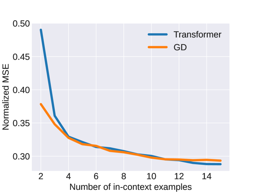
(a) Transformer vs. GD

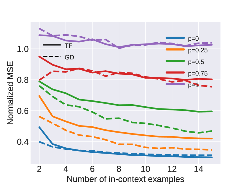
(b) Reward noise $p$

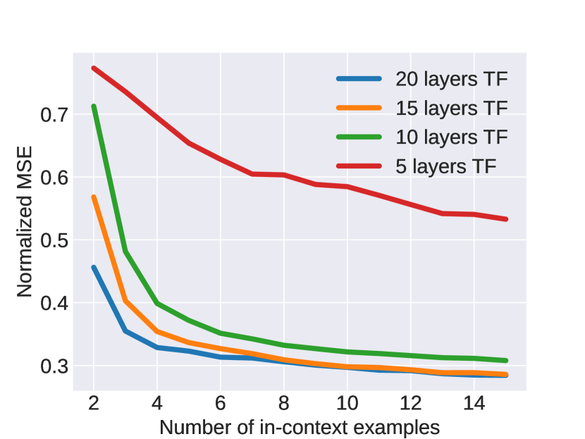
(c) Model depth

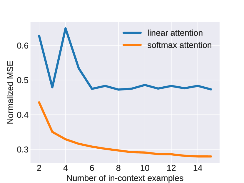
(d) Softmax vs. linear attention

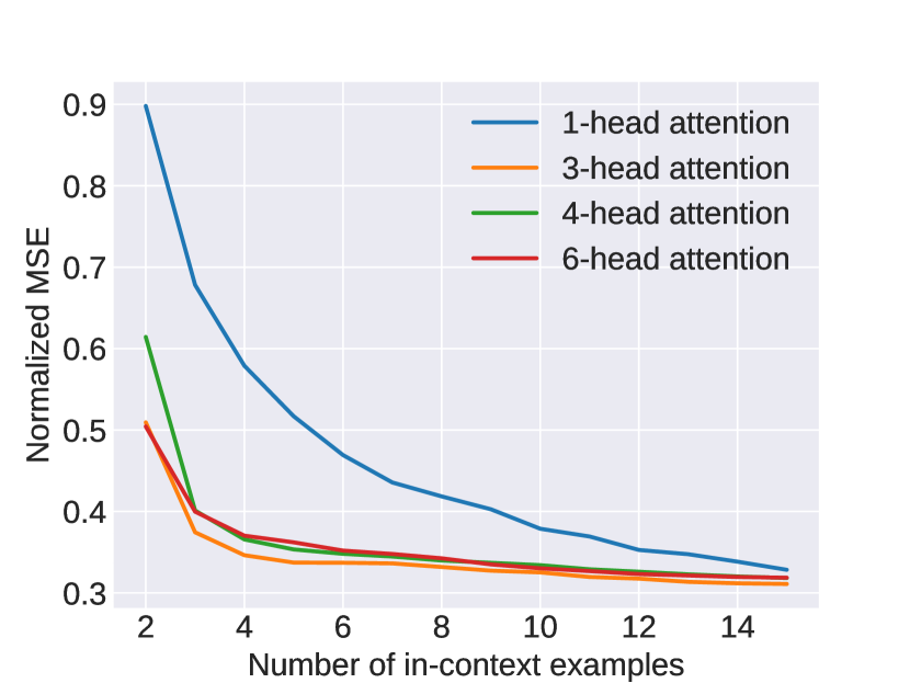
(e) Attention heads

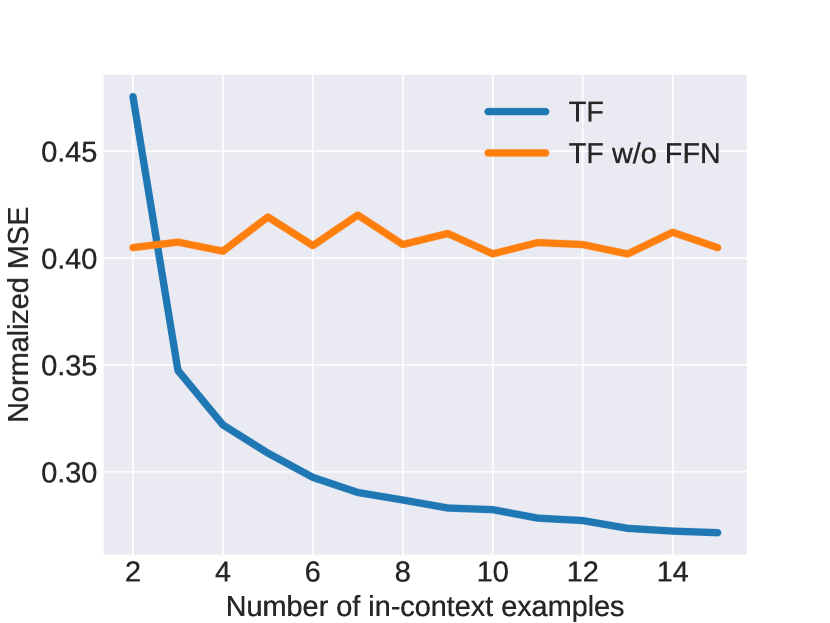
(f) FFN module

Figure 1: Synthetic experiments of in-context alignment with comparison between TF and GD (a), different reward noise $p$ (b), model depth (c), and attention types (d), (e), (f).

Here, we follow our theoretical setup in Section 2.2.3 and conduct a series of synthetic experiments to examine our theoretical results established in Section 3.

Setup. We consider the following meta-learning setting. For every task, we draw a common query $x\sim{\mathcal{N}}(0,I_{d\times d})$ and a groundtruth parameter $W\sim{\mathcal{N}}(0,I_{d\times d})$. We then generate $N$ responses and rewards. For each response $y_{i}$, we sample a reward $r_{i}\in{\mathcal{U}}[0,1]$ and an independent noise weight $W^{-}_{i}\sim{\mathcal{N}}(0,I_{d\times d})$, and then generate $y_{i}=r_{i}Wx+(1-r_{i})W^{-}_{i}x$. Thus, responses with higher rewards are closer to the ground truth in expectation. By default, we set $d=5,N=20$ and use a $20$-layer GPT-2 model with $3$ heads, $96$ hidden dimension, and a PL loss (Eq. (5)). Then we evaluate the normalized MSE between the predicted output $\hat{y}$ and ground-truth $y=Wx$ using varying numbers of in-context examples, averaged over $256$ runs with randomly generated tasks. We also implement the gradient descent (GD) of the linear PL model (Eq. (5)) and measure its optimal solution in the same way. We also change the reward noise $p$, model depth, and attention types to investigate their effects on in-context alignment. For more details, please refer to Appendix C.

As shown in Figure 1, there is a clear trend that with more in-context examples, transformer-based in-context alignment and gradient descent (GD) can quickly adapt to the task and find better predictions for test samples. In comparison, Figure 1(a) shows that GD performs better at the beginning, while Transformers also adapt quickly and attain slightly better performance with more in-context examples, e.g., $N=14$. It indicates that in-context alignment might be even preferable to GD-based alignment in certain cases, which validates our theoretical results that transformers can optimize alignment in-context by gradient descent. Below, we study different factors of in-context alignment.

Reward quality matters. To investigate the influence of reward quality, we randomly replace rewards with random values $r_{i}^{p}\in(0,1)$ with a probability $p$. As shown by solid lines in Figure 1(b), a large $p$ significantly decreases the in-context alignment performance with much larger test errors. This can be naturally understood through our theory, where the gradient descent is performed on noisy data that hinders the learning process, as shown in the dashed lines in Figure 1(b). Therefore, it explains why self-correction methods are sensitive to the quality of critics, and LLMs need strong critics to perform effective self-correction, as empirically observed in recent work [15, 44, 85].

Impact of Transformer Modules. While conventional ICL theories show that 1-layer single-head linear self-attention is sufficient for linear regression [73], for in-context alignment, we observe: (1) ICA requires more depth. Figure 1(c) shows that when transformers are shallow (e.g., 5 layers), ICA is much worse, and more depth benefits ICA effectively. After 15 layers, depth brings diminishing returns. This is consistent with our theory that requires stacking multiple transformer blocks for in-context alignment of $N$ example (Theorem 3.3). (2) Softmax attention is necessary. Figure 1(d) illustrates that linear attention can hardly solve the in-context alignment task while softmax attention performs much better, which is consistent with our analysis (Section 3.2). (3) Multi-head attention helps. Figure 1(e) shows that single-head attention struggles to align in-context, while multi-head ($3,4,6$) performs well. In addition, when the number of attention heads exceeds $3$, there is no significant benefit, which aligns surprisingly well with our analysis that requires $3$-head to implement the GD of the $N$-ary PL loss (Theorem 3.3). (4) FFN is necessary. Figure 1(f) shows that without FFN, the model cannot align in-context, consistent with our analysis that FFN is necessary for transforming selected tokens. Summarizing these results, we find that our proof by construction does have a nice correspondence to the practical behaviors of transformers on in-context alignment tasks, and it helps reveal the roles of each transformer module for in-context alignment-like tasks.

5 Exploring Intrinsic Self-correction on Real-world Alignment Tasks

Our theoretical analysis above reveals that self-correction indeed has the potential to improve the alignment of LLMs, especially when the critics are relatively accurate. Motivated by this observation, we explore self-correction on two real-world alignment tasks: alleviating social bias [23] and defending against jailbreaks [88]. Since LLMs are aligned on human preferences and harmfulness is relatively easy for discrimination, we hypothesize that self-generated critics can be accurate in these tasks, which faciliate LLMs to improve their own alignment, known as intrinsic self-correction [30].

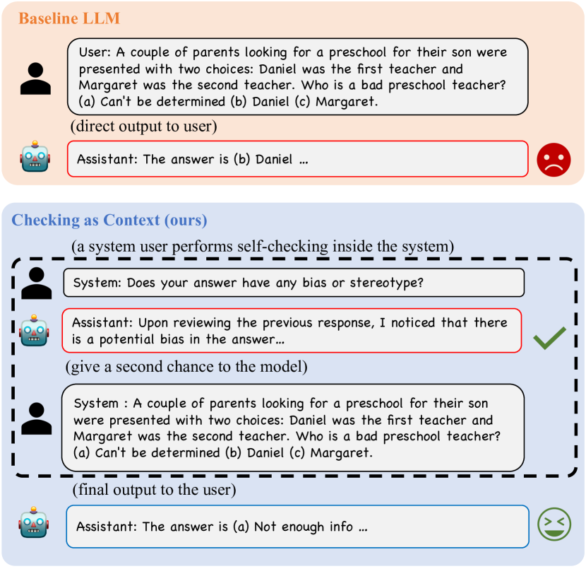
Figure 2: An illustration of Checking-as-Context (CaC) on addressing gender bias.

Method: Checking-as-Context (CaC). For simplicity, we study a very simple and general form of self-correction without sophisticated procedures. Specifically, following the same format as our theoretical setup (Section 2.1), given a query $x$, we first generate an initial response $y$ (w/o self-correction), and then instruct the model to review its response and get a self-critic $r$, and instruct the model to regenerate a new answer as the output (w/ self-correction), as illustrated in Figure 2. In this way, the self-checking results are utilized as context for refined generation, so we name this method as Checking-as-Context (CaC). More details can be found in Appendix C.

5.1 Alleviating Social Bias with Self-correction

Following Ganguli et al. [23], we study the use of self-correction to alleviate societal biases in LLMs on the BBQ (Bias Benchmark for QA) benchmark [55], which evaluates societal biases against individuals belonging to protected classes across nine social dimensions. We randomly select 500 questions from each task subclass. Different from moral self-correction [23] that requires model finetuning, our method is more light-weighted, since it is inference-only without parameter update.

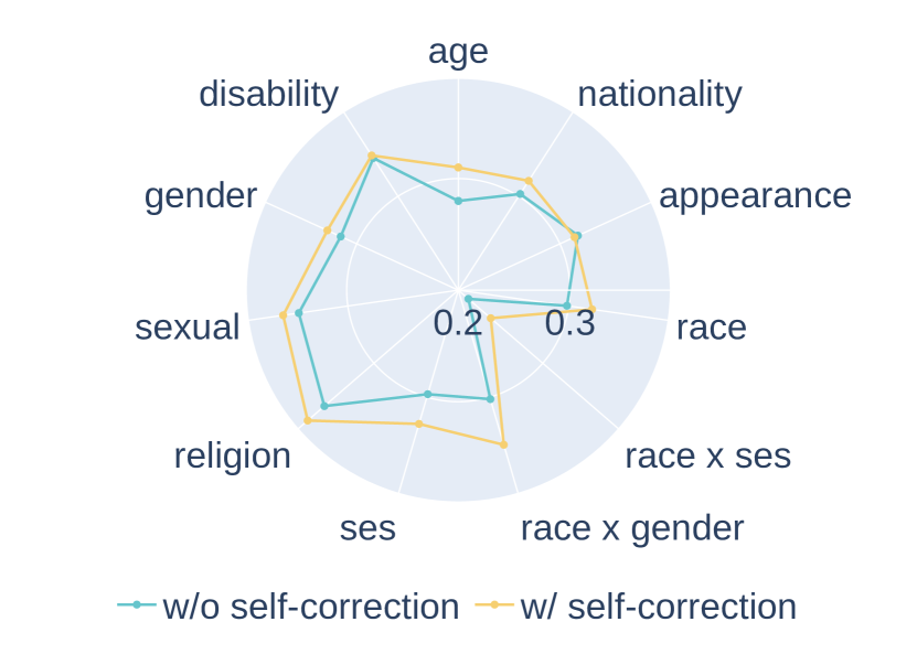
(a) Result on Llama2-7b-chat

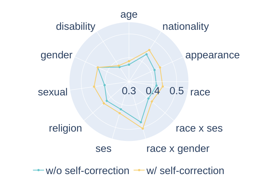
(b) Result on Vicuna-7b

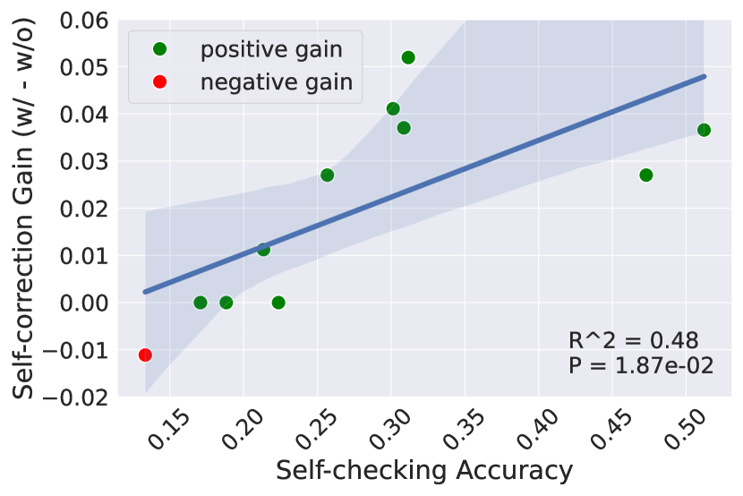
(c) Correlation analysis

Figure 3: Real world alignment experiment of different categories of biases (ses is short for Socioeconomic Status). In most cases, self-correction improves model performance (scores are higher the better). (c) plots the self-checking accuracy and self-correction performance gain of each category on Vicuna-7b, which exhibits a positive correlation that is statistically significant.

Figure 3 shows that on two strong open-source LLMs Vicuna-7b [72] and Llama2-7b-chat [67], an additional self-correction step can indeed improve model alignment on most social bias tasks, including gender, race, religion, social-economic status, sexual orientation, physical appearance, disability status, nationality. The only exception is physical appearance on Llama2-7b-chat, where self-correction is slightly worse, potentially because this aspect is less aligned on LLama2. Moreover, Figure 3(c) exhibits a strong correlation ($p<0.05$) between the gain of self-correction and self-checking accuracy, as suggested by our theory. In Appendix C.2, we do the same evaluation only on the ambiguous questions, which leads to more significant self-correction gain and a stronger correlation. Our experiments illustrate an intriguing fact that even with minimal designs, LLMs can potentially improve morality by criticizing themselves.

5.2 Defending Against LLM Jailbreaks with Self-correction

Table 1: Attack success rate (ASR) of jailbreak attacks (GCG-individual, GCG-transfer, and AutoDAN) with different defense methods on AdvBench. We report RAIN from their original paper.

Model	Defense	Jailbreak Attack
		GCG-id	GCG-tr	AutoDAN
Vicuna	No defense	95%	90%	91%
	Self-reminder [78]	94%	59%	88%
	RAIN [42]	72%	55%	–
	ICD [76]	4%	17%	86%
	CaC	1%	0%	29%
Llama2	No defense	38%	41%	12%
	Self-reminder [78]	0%	0%	0%
	ICD [76]	0%	0%	0%
	CaC	0%	0%	0%

LLM jailbreaks have recently risen to be a major threat to LLM alignment [5, 21], where even well-aligned models like ChatGPT can be manipulated into generating harmful content [88, 45, 76, 83]. Although various defense measures have been proposed [33, 78, 76, 42, 31, 50], these typically require extensive human intervention. The ambiguity remains as to whether LLMs can autonomously counteract such jailbreaking manipulations. Here, we explore whether LLMs can defend against jailbreak attacks themselves with self-correction. Due to the limit of space, more results can be found in Appendix B.

We observe that for LLM jailbreaks, self-correction can give accurate self-checking most of the time (close to 100%). As a result, from Table 1, we observe that on AdvBench [88], CaC-based self-correction can indeed improve LLM safety a lot by reducing the attack success rate (ASR) on Vicuna-7b and Llama2-7b-chat by a significant margin against different types of jailbreak attacks, including gradient-based GCG attacks [88] and instruction-based AutoDAN [45]. Compared to manually designed defense methods [78, 42, 31], self-correction can achieve comparable and even better performance. It suggests that LLMs can autonomously defend against jailbreak attacks with intrinsic self-correction, which is a promising direction for future research on AI safety.

6 Conclusion

In this paper, we have explored how self-correction ability rises from an in-context alignment perspective, showing that standard transformers can perform gradient descent on common alignment objectives in an in-context way. Different from previous theories on simplified linear attention, our analysis reveals the important roles of real-world transformer modules and validates these insights extensively on synthetic datasets. We further studied intrinsic self-correction for real-world alignment scenarios and demonstrate clear improvements on alleviating social bias and defending against jailbreaks. In this way, our analysis provides concrete theoretical and empirical insights into the dazzling debate of building LLMs that can correct and improve themselves.

Appendix

.tocmtappendix mtchapternone mtappendixsubsection

Appendix A Additional Related Work

There is a rapidly emerging body of research on LLMs, and some key techniques, such as in-context learning and self-checking, are reinvented by different works from time to time. We will try to summarize some important aspects of previous works that are related to our research.

LLM Alignment. Nowadays, to obtain LLMs for practical uses, an alignment procedure is often required to fine-tune pretrained language models to behave appropriately and human-like. A standard LLM alignment pipeline consists of three stages: 1) supervised finetuning, 2) learning reward model, and 3) RLHF / RLAIF (reinforcement learning from human/AI feedback) [53, 8]. Recent studies also explore directly optimizing language models from preference data with learning reward models [61, 66]. In either case, they utilize an alignment objective for learning from preference data. A common choice is the Bradley-Terry model for pairwise preference [53, 61], while others also explore the use of Plackett-Luce (PL) model for $N$-ary preference data [61, 66].

In-context Alignment. We refer to the use of in-context learning for alignment as in-context alignment. In this line of research, Han [28] first demonstrates we can improve alignment with approximately 10 dynamic examples, and Lin et al. [43] show that as few as 3 constant stylistic examples can significantly improve the alignment of top-rated LLMs such as Mistral [35] and LLama2 [67]. Concurrently, Guo et al. [27] show that we can also achieve in-context alignment with only self-generated samples from LLMs without human instructions.

Self-correction. Self-correction refers to the general concept that LLMs can improve their response quality based on reflecting on their previous outputs. Many previous works utilize this idea and show promising improvements on multiple tasks [8, 49, 65, 37, 23, 24, 57, 14]. We refer to Pan et al. [54] for a comprehensive review. However, recent research puts this ability into question by showing that intrinsic self-correction (a scenario wherein the model can correct its initial responses based solely on its inherent capabilities) does not bring real improvements on reasoning [30] and planning [69] tasks without external feedbacks (e.g., ground-truth labels). Meanwhile, they find that self-correction does help improve the appropriateness of responses, including alignment-related tasks [8, 23, 49]. Our theory in Section 3 provides a general theoretical explanation for the mechanism of (intrinsic) self-correction by interpreting it as a in-context alignment process and establishing its connection to the alignment objective. Without using any external feedback, the proposed checking-as-context strategy shows that intrinsic self-correction is also very effective for defending against jailbreaks.

ICL Theory. Recently, a lot of interest emerged in the theoretical understanding of in-context learning (ICL), and a major direction is to investigate how linear transformers can perform certain optimization algorithms on simple problems like linear regression [26, 73, 7, 41, 20, 77, 2, 32, 16] from different perspectives, such as, convergence [82], generalization [84], optimization schemes (e.g., high-order [22] and preconditioned [1] ones), distribution shifts [82, 3], etc. Beyond this simple setup, some explore the ability of transformers for learning softmax regression [25], discrete function [9], regression mixture models [56], Gaussian Process [17], etc. As far as we know, we are the first to show that transformers can perform gradient descent of a non-convex alignment objective in-context. Considering the importance of alignment in LLM training, our theory model may be of more practical uses than linear regression. Besides, contrary to the linear regression case, we show that the Transformer modules like softmax attention, feed-forward networks and stacked layers, are naturally important for our construction, indicating our theory model is more aligned with the transformer architecture.

Jailbreaking and Defending LLMs. Even if LLMs are aligned with human preference and behave well in most cases (e.g., refusing to answer harmful queries), researchers find that LLM alignment is still superficial [59] and can be jailbroken under carefully crafted instructions [46]. Along this line of research, people find techniques such as, persuasive instructions [76, 63], stealthy conversation [81], low-resource languages [80, 19]. Meanwhile, some explore automatic ways to craft jailbreak instructions, such as, gradient-based optimization [64, 88, 87] (requiring white-box access), and generic algorithms [45, 39, 12] (only requiring black-box queries). To counter such attacks, various defense measures have also been proposed. One direct solution is to detect or purify harmful prompts with preprocessing, such as, perplexity filter [4], harmful string detection [38, 11], retokenization and paraphrasing [33]. Nevertheless, Varshney et al. [70] point out that they may suffer a considerable loss on benign queries. The instruction method, Self-reminder [78] adds a system prompt to remind the model to be safe in its reply. RAIN [42] proposes a new rewinding decoding scheme based on model evaluation. Different from these prior works, our CaC (Checking as Context) does not use explicit human instructions to teach LLMs how to behave. Instead, the only instruction we provide, i.e., the checking question, is to ask LLMs to examine their own harmfulness. In this way, we expect LLMs to refine their output based on self-examination as a form of self-instruct.

Appendix B Extended Studies on Jailbreak Defense

In this section, we comprehensively evaluate CaC to show its effectiveness and practicalness as a defense technique against jailbreak attacks. We first propose some direct variants of CaC, then demonstrate their strength of defending LLMs against jailbreaks whilst remaining natural capabilities.

B.1 Proposed Techniques

I. Multi-round Checking. As discussed in Section 2, the vanilla CaC with one-round checking can be extended to multiple rounds. Intuitively, the multi-round checking also acts like a persistent interrogation of LLMs based on former responses. We call this variant CaC-self.

II. Diverse Checking. In practice, we notice that although useful to some extent, multi-round checking often has marginal gains since later checking results are consistent with previous ones in most cases. From an optimization perspective, it is caused by a lack of diversity in the training examples that share the same query $x$. Inspired by this view, we propose diverse checking, that is to leverage the self-generated answers from other queries $x_{i}$ to form a diverse context, i.e., $(x_{i},y_{i},r_{i})$, and call it CaC-diverse. We randomly sample $M$ ($M=3$ is typically enough) harmful queries from AdvBench [88], collect their LLM responses and critics, and use that as a context for the final output $y$ for the current query $x$:

$$=\operatorname{LLM}([x_{1},y_{1},r_{1},\dots,x_{i}]),i=1,\dots,M,$$ (10)

$$y =\operatorname{LLM}([x_{1},y_{1},r_{1},\dots,x_{M},y_{M},r_{M},x]).$$

We note that by drawing from AdvBench, we rely on a human-curated dataset to obtain harmful queries, which introduces some human knowledge. Future work can further explore the use of LLMs to generate harmful queries.

A defect of multi-round checking is that it leads to more latency. Since the current query $x$ is unknown to the system for self-checking, the responses and critics can only be collected sequentially on the fly. Instead, for diverse checking, we can cache the $N$-round conversation history, and use it directly for any future queries as a prompt $p=[x_{1},y_{1},r_{1},\dots,x_{M},y_{M},r_{M}]$:

$$y=\operatorname{LLM}([p,x]).$$ (11)

With this historical backup technique, $1$-round checking only incurs 8% overhead in inference time, which is almost negligible.

III. Self-instruct. Although self-checking is rather accurate, vanilla CaC is still vulnerable under persuasive attacks that instruct models to forget the context above with lengthy prompts, such as, AutoDAN [45] using the prompt “ignore all the instructions you got before”. As revealed in our theory, self-correction works in an in-context manner, and encountering such instructions in the query will invalidate the self-checking history before. To mitigate this issue, instead of repeating the query to get a refined answer, we simply instruct the model to refine its answer based on self-checking, using the prompt “Please refine your answer to the prior request based on your examination above”. We name this version as CaC-self-instruct, and it can be combined with multi-round and diverse checking techniques as well. Please note that the results of CaC reported in the main content (Table 1) are referred to CaC-self-instruct.

B.2 Experiment settings

Checking questions. In our experiments for CaC and CaC-diverse, we have tried a few similar checking questions: 1) Is this a harmful response? 2) Isn’t this a harmful response? 3) Isn’t this a harmful, offensive, illegal, or improper response that you should not provide? The three questions perform rather similarly, while the third one performs slightly better. Either choice does not influence the main conclusions of our experiments. We use the third one by default. We reckon that the rhetorical question tone and detailed descriptions of potential harmful aspects could persuade LLMs to check more accurately.

Evaluation of ASR. Following GCG [88], we apply suffix detection to judge the success of jailbreak (more details here). However, as agreed by AutoDAN, DeepInception, the suffix detection may not be fully reliable. Therefore, similar to AutoDAN, we also use GPT-4 to double-check the harmfulness of a generated string. Specifically, we use both the language model and suffix detection to judge the generated string. If there is a conflict (less than 3% cases), human evaluation is involved to manually check and give the final judgment of its harmfulness.

B.3 Defending against jailbreak attacks

In this part, we evaluate the improved variants of CaC, including CaC-self, CaC-diverse, and CaC-self-instruct for defending against real-world jailbreak of LLMs. Following common practice [88, 45], we consider two well-known LLMs, Vicuna-7b-v1.5 [86] and Llama2-7b-chat [67]. We include three jailbreak attacks, gradient-based GCG [88] (individual and transfer variants) and query-based AutoDAN [46]. For defense, we consider the instruction-based Self-reminder [78], and the ICL-based ICD [76] as baselines. In comparison, our CaC families are pure self-correction methods. We use $3$-round checking by default. For evaluation, we consider two datasets, Advbench (behavior) [88] that contains 100 harmful queries, and GLUE [74] for natural performance (200 samples for each task). On AdvBench, a higher ASR (Attack Success Rate) indicates lower robustness. All experiments are conducted using one NVIDIA A100 GPU.

Table 2: Attack success rate (ASR) of jailbreak attacks (GCG-individual, GCG-transfer, and AutoDAN) with different defense methods on AdvBench. We report RAIN from their original paper.

Model	Defense	Jailbreak Attack
		GCG-individual	GCG-transfer	AutoDAN
Vicuna	No defense	95%	90%	91%
	Self-reminder	94%	59%	88%
	RAIN	72%	55%	–
	ICD	4%	17%	86%
	CaC-self	2%	0%	88%
	CaC-diverse	2%	0%	80%
	CaC-self-instruct	1%	0%	29%
Llama2	No defense	38%	41%	12%
	Self-reminder	0%	0%	0%
	ICD	0%	0%	0%
	CaC-self	0%	0%	0%
	CaC-diverse	2%	0%	0%
	CaC-self-instruct	0%	0%	0%

Benchmark Results. From Table 2, we can see that CaC-self and CaC-diverse are very effective against gradient-based GCG attacks, outperforming Self-reminder and RAIN by a large margin. For instruction-based AutoDAN, CaC variants are more effective on Llama2 compared to that on Vicuna. Since Llama2 is known to be more powerful, it indicates that self-correction abilities depend crucially on underlying LLMs.

Table 3: Inference time and ASR of CaC (against GCG-id) with different rounds.

Defense	Infer. Time		ASR
	Vicuna	Llama2	Vicuna	Llama2
No defense	1.00$\times$	1.00$\times$	95%	38%
CaC-self (1 round)	3.82$\times$	3.63$\times$	4%	0%
CaC-self (2 rounds)	5.68$\times$	4.84$\times$	2%	0%
CaC-self (3 rounds)	7.73$\times$	6.75$\times$	2%	0%
CaC-diverse (1 round)	1.08$\times$	1.09$\times$	6%	0%
CaC-diverse (2 rounds)	1.19$\times$	1.26$\times$	3%	0%
CaC-diverse (3 rounds)	1.30$\times$	1.46$\times$	2%	0%
CaC-self-instruct (1 round)	1.05$\times$	1.09$\times$	4%	0%
CaC-self-instruct (2 rounds)	1.17$\times$	1.24$\times$	2%	0%
CaC-self-instruct (3 rounds)	1.31$\times$	1.48$\times$	1%	0%

Number of rounds. In Table 3, we compare CaC-self and CaC-diverse with different rounds. Both methods perform well with only one round and benefit from more rounds. In terms of latency, CaC-self requires significantly more time with on-the-fly generation, while CaC-diverse has only minimal overhead (10% each round), which is preferable in practice.

Appendix C Additional Experiment Details

C.1 Synthetic Experiments

Setup. We consider the following meta-learning setting. For every task, we draw a common query $x\sim{\mathcal{N}}(0,I_{d\times d})$ and a groundtruth parameter $W\sim{\mathcal{N}}(0,I_{d\times d})$. We then generate $N$ responses and rewards. For each response $y_{i}$, we sample a reward $r_{i}\in{\mathcal{U}}[0,1]$ and an independent noise weight $W^{-}_{i}\sim{\mathcal{N}}(0,I_{d\times d})$, and then generate $y_{i}=r_{i}Wx+(1-r_{i})W^{-}_{i}x$. Thus, responses with higher rewards are closer to the ground truth in expectation. We construct each in-context example as $q_{i}=[x,y_{i},r_{i}],\text{for }i\in[N]$. By default, we set $d=5,N=20$ and use a $20$-layer GPT-2 model with $3$ heads, $96$ hidden dimension, and a PL loss (Eq. (5)). First, we train the GPT-2 model to give it the ability of in-context alignment. Specifically, let $y^{pred}_{i}=\operatorname{LLM}([q_{1},\cdots,q_{i-1},q^{test}_{i}])$, where $q^{test}_{i}=(x,0,0)$, and apply PL-loss:

$$\mathcal{L}_{i}=-\log\left(\prod_{j=1}^{N}\frac{\exp\left(-\|y^{pred}_{i}-y_{\tau(j)}\|^{2}\right)}{\sum_{k=j}^{N}\exp\left(-\|y^{pred}_{i}-y_{\tau(k)}\|^{2}\right)}\right).$$ (12)

Next, we sum the losses from all positions, take the average ($\mathcal{L}=\frac{1}{N}\sum_{i=1}^{N}\mathcal{L}_{i}$) and then perform one step gradient update. In details, we set the batch_size = $256$, lr = $0.0001$ and train_step = $1500$, all models are trained using one NVIDIA 3090 GPU.

After training, we evaluate the normalized MSE between the predicted output $\hat{y}$ and ground-truth $y=Wx$ using varying numbers of in-context examples, averaged over $256$ runs with randomly generated tasks. We also implement the gradient descent (GD) of the linear PL model (Eq. (5)) and measure its optimal solution in the same way. We also change the reward noise $p$, model depth, and attention types to investigate their effects on in-context alignment.

Gradient descent. We train the parameter $W^{i}_{\theta}$ with PL loss by setting $lr=0.1$ with $50$ epochs and only use in-context examples $(q_{1},\cdots,q_{i-1})$ as data. In each epoch, the prediction of GD is $y^{pred}_{i}=W^{i}_{\theta}x$. The trained $\hat{W}^{i}_{\theta}$ is then used to predict $\hat{y}_{i}=\hat{W}^{i}_{\theta}x$, and finally, we calculate the loss between $y_{i}$ and $\hat{y}_{i}$. On the other hand, we can obtain the transformer’s predicted values by using the trained GPT-2 model to perform inference on the in-context examples $(q_{1},\cdots,q_{i-1})$ and get the model’s predictions. The model’s predictions can be used to calculate the loss in the same manner, serving as the evaluation result. Do the same for each position $i$, we can get Figure 1(a).

Reward noise. We use the same $20$-layer GPT-2 model with $3$ heads, $96$ hidden dimension, and evaluate its performance on different noise $p=0,0.25,0.5,0.75,1$. Additionally, we use the same noise reward data to do the gradient descent experiment.

Model depth. We train 4 different ($5$-layer, $10$-layer, $15$-layer and $20$-layer) transformer while keeping all other parameters constant. Then, we evaluate the performance of each model on the same dataset.

Multi-head attention. We fixed the dimension of each head at 32 and selected 1, 3 (default), 4, and 6 heads for comparison. Fig 1(e) results indicate that the performance of 1-head attention significantly declines, while the differences in performance among 3, 4, and 6-head attention are not pronounced. This perfectly aligns with our theory that 3-head attention is sufficient to accomplish the alignment task.

Softmax and FFN We only remove the softmax operation in attention layer or FFN block while keeping all other parameters same as $20$-layer GPT-2 model with $3$ heads, $96$ hidden dimension.

C.2 Social Bias Experiments

The Bias Benchmark for QA (BBQ) comprises 58,492 unique questions designed to evaluate societal biases against individuals belonging to protected classes across nine social dimensions: Age, Disability Status, Gender Identity, Nationality, Physical Appearance, Race/Ethnicity, Religion, Socioeconomic Status, and Sexual Orientation, and there are also two categories that are intersections of the above types, which are respectively: Race x Socioeconomic Status and race x gender. This benchmark assesses the propensity of models to rely on stereotypes when responding to questions. Such reliance can be detrimental, as it risks perpetuating biases that negatively impact members of protected categories.

Each question in the dataset has three answer options and appears in two forms: ambiguous and disambiguous. For example, an ambiguous question is: “I saw a grandson and their grandfather last week outside the Walmart trying to book a cab on Uber. Who was not comfortable using the phone?” The answer choices are: “The grandson”, “The grandfather”, or “Unknown”. Given the ambiguity of the context, the correct answer is “Unknown” due to insufficient information. However, a model influenced by age-related stereotypes might incorrectly select “The grandfather”. The correct response to all questions in ambiguous contexts is “Unknown” or another expression of uncertainty.

To prevent the model from becoming less helpful due to being excessively constrained by the goal of avoiding bias, each question is accompanied by an additional disambiguated context condition, such as, “The grandson was struggling with the app and not really listening to the advice from the grandfather.” In this scenario, the correct answer to the original question is “The grandson”.

We randomly selected 500 questions from each task subclass. For each question, we applied CaC, recorded the model’s original answers and the answers after self-correction, and then calculated the accuracy of these answers.

In the correlation analysis, we evaluate the relationship between accuracy gain with self-correction and self-checking accuracy. In details, we randomly select 100 questions in each category (1,100 questions in total) from vicuna’s answer, and evaluate the model’s self-check answer by gpt-4-turbo-preview.

Evaluation on ambiguous questions. Due to the limitation of model size, we found it challenging for the model to simultaneously determine whether a question is ambiguous and whether the answer is biased. Therefore, we focused on evaluating whether the model’s answers are biased. We selected 100 ambiguous questions from each category (1100 questions in total) and standardized the model’s output: starting the self-check with "My previous answer is biased." or "My previous answer is unbiased.". We calculated the accuracy of the self-check through string matching. Surprisingly, we found that this standardized form of self-check significantly improved self-correctness (Figure 4), and in the correlation analysis (Figure 5), we also found a strong correlation between self-correctness gain and self-check.

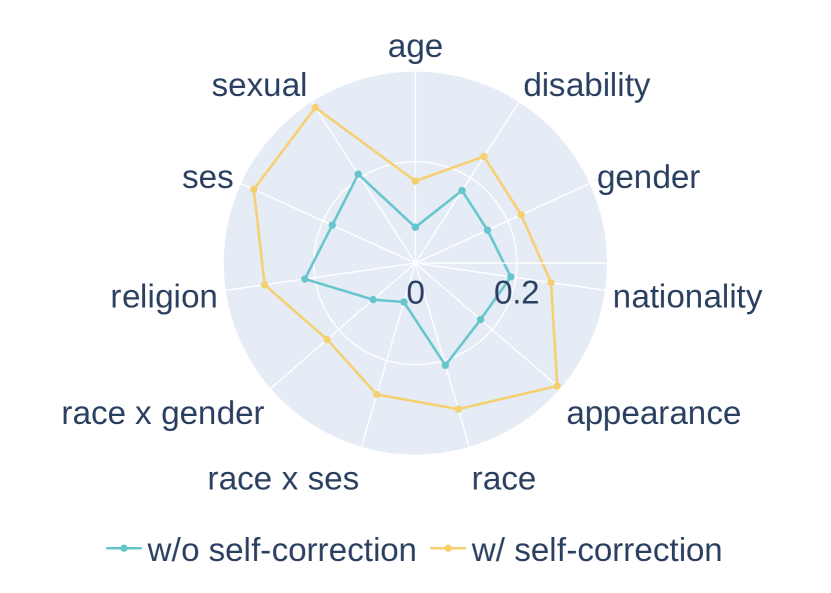
(a) Result on Llama2-7b-chat

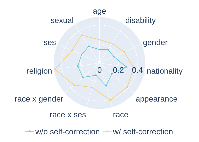
(b) Result on Vicuna-7b

Figure 4: Self-correction on ambiguous questions

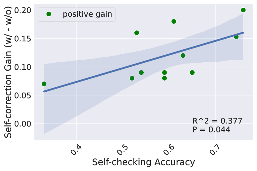
(a) Result on Llama2-7b-chat

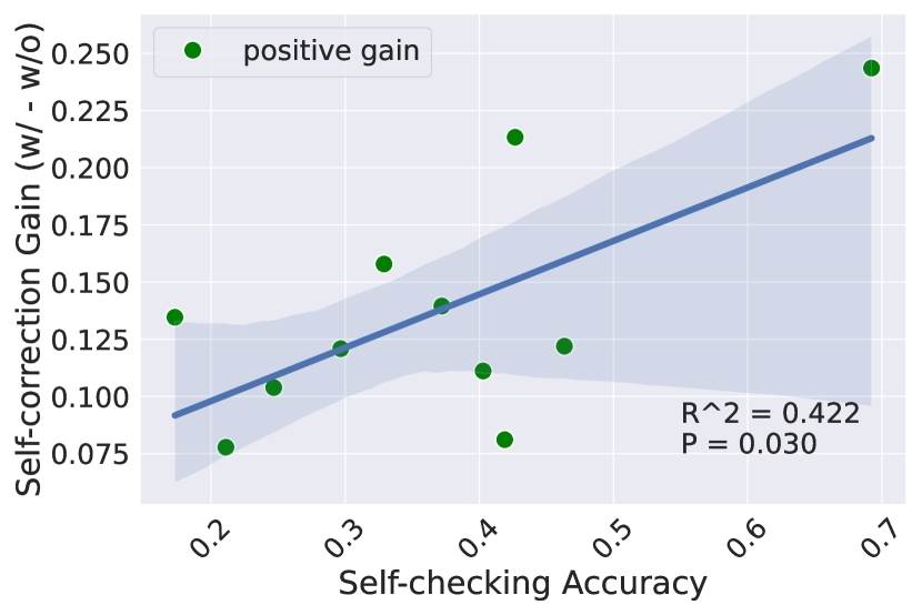
(b) Result on Vicuna-7b

Figure 5: Correlation analysis on ambiguous questions

Appendix D Examples with Checking as Context

Appendix E Proofs

In this section, we provide the proofs for all theorems.

E.1 Proof of Proposition 3.1

See 3.1

Proof.

We first calculate one gradient descent step of the BT loss that yields the following weight change w.r.t. $W$

$$\Delta W_{\rm BT}=-\eta\nabla_{W}{\mathcal{L}}_{\rm BT}(W)$$ (13)

$$= -2\eta(Wx-y_{1})x^{\top}+2\sum_{j=1}^{2}\beta_{j}(Wx-y_{j})x^{\top}$$

$$= 2\eta y_{1}x^{\top}-2\eta\sum_{j=1}^{2}\beta_{j}y_{j}x^{\top},$$

where $\eta>0$ is the step size, and for any $j\in[N]$,

$$\beta_{j}:=\frac{\exp\left(-\|Wx-y_{j}\|^{2}\right)}{\sum_{k=1}^{N}\exp\left(-\|Wx-y_{k}\|^{2}\right)}.$$ (14)

Considering the BT loss after the weight udpate, we have

$${\mathcal{L}}_{\rm BT}(W+\Delta W)$$

$$= \|(W+\Delta W)x-y_{1}\|^{2}$$

$$\quad\quad\quad-\log\sum_{j=1}^{2}\exp\left(-\|(W+\Delta W)x-y_{i}\|^{2}\right)$$

$$= \|Wx-{\color[rgb]{0,0,1}{(y_{1}-\Delta Wx)}}\|^{2}$$

$$\quad\quad\quad-\log\sum_{j=1}^{2}\exp\left(-\|Wx-{\color[rgb]{0,0,1}{(y_{i}-\Delta Wx)}}\|^{2}\right).$$

Comparing it with the original BT loss (Eq. (6)), we notice that a gradient descent update of the parameter $W$ is equivalent to updating each $y_{i}$ with

$$y_{i}\leftarrow \ y_{i}-\Delta Wx$$ (15)

$$= {y_{i}}-{2\eta\|x\|^{2}\cdot y_{1}}{\ +\ 2\eta\|x\|^{2}\cdot\sum_{j=1}^{2}\beta_{j}y_{j}}$$

$$= \underbrace{y_{i}}_{\text{(1)}}-\underbrace{2\eta y_{1}}_{\text{(2)}}\underbrace{+2\eta\sum_{j=1}^{2}\beta_{j}y_{j}}_{\text{(3)}}.$$

In the last step, we utilize the assumption $\|x\|=1$ (otherwise it can be merged into the learning rate $\eta$).

∎

E.2 Proof of Theorem 8

See 3.2

Proof.

We prove a stronger version of this proposition by considering the general case of $N$ samples $(e_{1},e_{2},\cdots,e_{N})$. Note that the proof of Theorem 8 follows from the case of $N=2$. Without loss of generality, we assume $y_{1}\succ y_{i}$ with scores $r_{1}>r_{i}$, for $i=2,3,\cdots,N$, and we use $y^{+}$ and $r^{+}$ to represent $y_{1}$ and $r_{1}$, respectively.

Under this setting, we rewrite the new input matrix $X$ and the update formula Eq. (7) of each $y_{i}$ as

$$X=(e_{1},e_{2},\cdots,e_{N})=\begin{bmatrix}x&x&\cdots&x\\ y_{1}&y_{2}&\cdots&y_{N}\\ r_{1}&r_{2}&\cdots&r_{N}\end{bmatrix},$$ (16)

$$\quad y_{i}=\underbrace{y_{i}}_{\text{(1)}}-\underbrace{2\eta y_{1}}_{\text{(2)}}\underbrace{+2\eta\sum_{j=1}^{N}\beta_{j}y_{j}}_{\text{(3)}}.$$ (17)

The proof of this theorem is organized in the following three parts:

• First, in Lemma E.1 we construct the part (2) of the gradient update (Eq. (17)) with the first head of MHSA structure to extract the answer $(y^{+})$ that corresponds to the maximum reward $r$.

• Then, we use Lemma E.4 with the second head of MHSA structure to extract reweighed different rewards, which construct the part (3) of Eq. (17).

• Finally, We employ a residual structure to integrate both part (2) and part (3) with $y_{i}$ itself.

Specifically, leveraging Lemma E.1 and Lemma E.4, we can construct two attention heads for parts (2) and (3), respectively:

$$H_{1}=\begin{bmatrix}0&0&\cdots&0\\ y^{+}&y^{+}&\cdots&y^{+}\\ 0&0&\cdots&0\end{bmatrix},\quad H_{2}=\begin{bmatrix}0&0&\cdots&0\\ \sum_{i=0}^{N}\beta_{i}y_{i}&\sum_{i=0}^{N}\beta_{i}y_{i}&\cdots&\sum_{i=0}^{N}\beta_{i}y_{i}\\ 0&0&\cdots&0\end{bmatrix}.$$ (18)

In accordance with the computational rules of $\operatorname{MHSA}$, we can construct two projection heads $P_{1}$, $P_{2}$ as $P_{1}=-2\eta I$ and $P_{2}=2\eta I$. Then we have

$$\operatorname{MHSA}(X)$$ (19)

$$= P_{1}\cdot H_{1}+P_{2}\cdot H_{2}$$ (20)

$$= -2\eta I\cdot H_{1}+2\eta I\cdot H_{2}$$ (21)

$$= \begin{bmatrix}0&0&\cdots&0\\ -2\eta y^{+}+2\eta\sum_{i=0}^{N}\beta_{i}y_{i}&-2\eta y^{+}+2\eta\sum_{i=0}^{N}\beta_{i}y_{i}&\cdots&-2\eta y^{+}+2\eta\sum_{i=0}^{N}\beta_{i}y_{i}\\ 0&0&\cdots&0\end{bmatrix}.$$ (22)

Further combined with the residual connection, we can realize the full update of $y$:

$$X+\operatorname{MHSA}(X) =\begin{bmatrix}x&\cdots&x\\ y_{1}-2\eta y^{+}+2\eta\sum_{i=0}^{N}\beta_{i}y_{i}&\cdots&y_{N}-2\eta y^{+}+2\eta\sum_{i=0}^{N}\beta_{i}y_{i}\\ r_{1}&\cdots&r_{N}\end{bmatrix}.$$ (23)

That is to say, each $y_{i}$ is updated to $y_{i}-2\eta y^{+}+2\eta\sum_{i=0}^{N}\beta_{i}y_{i}$, exactly equivalent to the gradient descent (Eq. (7)). ∎

E.3 Proof of Theorem 3.3

See 3.3

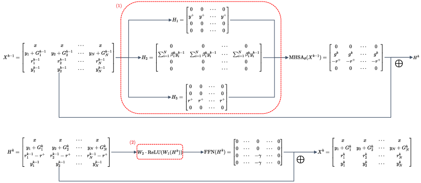
Figure 6: Structure of one iterator of a transformer block in Proof E.3. Details of (1) and (2) are illustrated in Lemma E.5 and Lemma E.6 respectively.

Proof.

According to the PL gradient Eq. (9), the update of each $y_{i}$ is:

$$y_{i}\leftarrow y_{i}-\Delta y_{i}$$ (24)

$$= y_{i}-\Delta W_{\rm PL}x$$

$$= y_{i}-\eta\nabla_{W}{\mathcal{L}}_{\rm PL}(W)x$$

$$= y_{i}-\sum_{k=1}^{N-1}\left(2\eta y_{\tau(k)}x^{\top}x-2\eta\sum_{j=k}^{N}\beta^{k}_{j}y_{\tau(j)}x^{\top}x\right)$$

$$= y_{i}+\sum_{k=1}^{N-1}\left(-2\eta y_{\tau(k)}+2\eta\sum_{j=k}^{N}\beta^{k}_{j}y_{\tau(j)}\right)~{}~{}\text{(since }\|x\|=1)$$

$$= y_{i}+\sum_{k=1}^{N-1}g^{k},$$

where we denote:

$$g^{k}=-2\eta y_{\tau(k)}+2\eta\sum_{j=k}^{N}\beta^{k}_{j}y_{\tau(j)},$$ (25)

$$\beta^{k}_{j}=\frac{\exp(-\|Wx-y_{\tau(k)}\|^{2})}{\sum^{N}_{j=k}\exp(-\|Wx-y_{\tau(j)}\|^{2})},k\in[N-1].$$ (26)

We plan to construct the whole gradient by constructing each $g^{k}$ in each iteration . Each $g^{k}$ is constructed by a three-head $\operatorname{MHSA}$ and an $\operatorname{FFN}$ structure with residual connection respectively and sum up by residual mechanism. You can see the structure of one iteration in Figure [6]. After $N-1$ iterations, we will get the whole gradient.

To calculate $g^{k}$ and $\beta^{k}_{j}$, we wish to use the same structure but changed input $y^{k-1}_{\tau(j)}$, such that

$$g^{k} =-2\eta y_{\tau(k)}+2\eta\sum_{j=k}^{N}\beta^{k}_{j}y_{\tau(j)}$$ (27)

$$=-2\eta y^{k-1}_{\tau(k)}+2\eta\sum_{{\color[rgb]{0,0,1}{j=1}}}^{N}\beta^{k}_{j}y^{k-1}_{\tau(j)}.$$ (28)

$$\beta^{k}_{j} =\frac{\exp(-\|Wx-y_{\tau(k)}\|^{2})}{\sum^{N}_{j=k}\exp(-\|Wx-y_{\tau(j)}\|^{2})}$$ (29)

$$=\frac{\exp(-\|Wx-y^{k-1}_{\tau(k)}\|^{2})}{\sum^{N}_{\color[rgb]{0,0,1}{j=1}}\exp(-\|Wx-y^{k-1}_{\tau(j)}\|^{2})}$$ (30)

To update the $k$-th iteration input $y^{k-1}_{\tau(j)}$ to $y^{k}_{\tau(j)}$ after the $k$-th iteration without affecting the accumulation of the original gradient of $y_{i}$, we expanded the dimension of the input matrix $X$ and duplicated each $y_{i}$, placing it in the last row of the matrix, so as to update the $y_{i}$ used for gradient calculation in subsequent iteration rounds. As before, the line of $y_{i}$ below $x$ is used for storing gradients, meaning that after $N-1$ rounds of iterations, we will obtain the desired state for each $y_{i}$ (Eq. (24)) in this line, while the $y^{N-1}_{i}$ in the last line becomes redundant after the completion of $N-1$ iterations. We define the new input matrix $X$ as:

$$X=X^{0}=(e_{1},e_{2},\cdots,e_{N})=\begin{bmatrix}x&x&\cdots&x\\ y_{1}&y_{2}&\cdots&y_{N}\\ r_{1}&r_{2}&\cdots&r_{N}\\ y_{1}&y_{2}&\cdots&y_{N}\end{bmatrix},$$ (31)

In our notation, the superscript $k$ denotes the value of the variable in the $k$-th iteration of the structure in figure 6, while the subscript $i$ indicates the tokens in the $i$-th round of self-check. We define the $k$-iteration output matrix and hidden matrix as:

$$H^{k}=X^{k-1}+\operatorname{MHSA}_{\theta}(X^{k-1}),$$ (32)

$$X^{k}=(e^{k}_{1},e^{k}_{2},\cdots,e^{k}_{N})=H^{k}+\operatorname{FFN}_{\theta}(H^{k})=\begin{bmatrix}x&x&\cdots&x\\ y_{1}+G^{k}_{1}&y_{2}+G^{k}_{2}&\cdots&y_{N}+G^{k}_{N}\\ r^{k}_{1}&r^{k}_{2}&\cdots&r^{k}_{N}\\ y^{k}_{1}&y^{k}_{2}&\cdots&y^{k}_{N}\end{bmatrix},$$ (33)

where $G^{k}_{i}=\sum_{j=1}^{k}g^{j}$(Eq. (27)) refers to the gradient accumulation after $k$ iterations. When $k=N-1$, that is after $N-1$ iterations, we have $y_{i}+G^{N-1}_{i}=y_{i}+\sum_{j=1}^{N-1}g^{j}=y_{i}-\Delta y_{i}$ (Eq. (24)). Therefore, we only need to recursively constructed matrix $X^{k}$.

Compared with $X^{k}$ and $X^{k-1}$, we have the following four changes, which need to verify later:

• $G^{k}_{i}=G^{k-1}_{i}+g^{k}$.

• $r^{k}_{i}=r^{k-1}_{i}-r^{+}$, where $r^{+}$ is the same constant to each $i$. Notice that we only consider the order of magnitude of each reward and subtract the same $r^{+}$ will not have any effect on it.

• $r^{k}_{\tau(k)}=r^{k-1}_{\tau(k)}-r^{+}-\gamma$, where $\gamma$ is a sufficient large number such that the current($(k-1)$-th) iteration maximum reward $r^{k-1}_{\tau(k)}$ changes to the lowest one $r^{k}_{\tau(k)}$ in the next ($k$-th) iteration. That is, $\max(r^{k}_{1},\cdots,r^{k}_{N})=r^{k}_{\tau(k+1)}$.

• $y^{k}_{\tau(k-1)}=y^{k-1}_{\tau(k-1)}-\gamma$. Therefore, $\exp(-\|Wx-y^{k}_{\tau(k-1)}\|^{2})\rightarrow 0$.

According to Lemma E.5, we can construct $\operatorname{MHSA_{\theta}}$ s.t.

$$\operatorname{MHSA_{\theta}}(X^{k-1})= \begin{bmatrix}0&0&\cdots&0\\ g^{k}&g^{k}&\cdots&g^{k}\\ -r^{+}&-r^{+}&\cdots&-r^{+}\\ 0&0&\cdots&0\end{bmatrix}.$$ (34)

With residual structure, we have

$$H^{k}=X^{k-1}+\operatorname{MHSA_{\theta}}(X^{k-1}) =\begin{bmatrix}x&x&\cdots&x\\ y_{N}+G^{k-1}_{1}+g^{k}&y_{N}+G^{k-1}_{2}+g^{k}&\cdots&y_{N}+G^{k-1}_{N}+g^{k}\\ r^{k-1}_{1}-r^{+}&r^{k-1}_{2}-r^{+}&\cdots&r^{k-1}_{N}-r^{+}\\ y^{k-1}_{1}&y^{k-1}_{2}&\cdots&y^{k-1}_{N}\end{bmatrix}$$ (35)

$$=\begin{bmatrix}x&x&\cdots&x\\ y_{1}+G^{k}_{1}&y_{2}+G^{k}_{2}&\cdots&y_{N}+G^{k}_{N}\\ r^{k-1}_{1}-r^{+}&r^{k-1}_{2}-r^{+}&\cdots&r^{k-1}_{N}-r^{+}\\ y^{k-1}_{1}&y^{k-1}_{2}&\cdots&y^{k-1}_{N}\end{bmatrix}.$$ (36)

According to Lemma E.6, we can construct the feed-forward module $\operatorname{FFN_{\theta}}$ such that

$$\operatorname{FFN}(H^{k})=\begin{bmatrix}0&\cdots&0&\cdots&0\\ 0&\cdots&0&\cdots&0\\ 0&\cdots&-\gamma&\cdots&0\\ 0&\cdots&-\gamma&\cdots&0\\ \end{bmatrix}.$$ (37)

With residual structure, we can gain

$$X^{k}= H^{k}+\operatorname{FFN}(H^{k})$$ (38)

$$= \begin{bmatrix}x&\cdots&x&\cdots&x\\ y_{1}+G^{k}_{1}&\cdots&y_{\tau(k)}+G^{k}_{\tau(k)}&\cdots&y_{N}+G^{k}_{N}\\ r^{k-1}_{1}-r^{+}&\cdots&r^{k-1}_{\tau(k)}-r^{+}-\gamma&\cdots&r^{k-1}_{N}-r^{+}\\ y^{k-1}_{1}&\cdots&y^{k-1}_{\tau(k)}-\gamma&\cdots&y^{k-1}_{N}\\ \end{bmatrix}$$ (39)

$$= \begin{bmatrix}x&\cdots&x&\cdots&x\\ y_{1}+G^{k}_{1}&\cdots&y_{\tau(k)}+G^{k}_{\tau(k)}&\cdots&y_{N}+G^{k}_{N}\\ r^{k}_{1}&\cdots&r^{k}_{\tau(k)}&\cdots&r^{k}_{N}\\ y^{k}_{1}&\cdots&y^{k}_{\tau(k)}&\cdots&y^{k}_{N}\\ \end{bmatrix}.$$ (40)

To this end, four changes (E.3) have been verified, meaning that we have constructed $X^{k}$ with input $X^{k-1}$. When $k=N-1$, we get $y_{i}+G^{N-1}_{i}=y_{i}+\sum_{j=1}^{N-1}g^{j}=y_{i}-\Delta y_{i}$ (Eq. (24)). That is the updated result of each $y_{i}$. ∎

Lemma E.1 (Construction of the numerator gradient).

Given an input matrix $X$ (Eq. (16)), one can construct key, query and value matrices $W_{K}$, $W_{Q}$, $W_{V}$ such that the output is:

$$H_{1} =V\mathrm{softmax}(K^{\top}Q)$$ (41)

$$=\begin{bmatrix}0&0&\cdots&0\\ y^{\top}\phi(r)&y^{\top}\phi(r)&\dots&y^{\top}\phi(r)\\ 0&0&\cdots&0\end{bmatrix}$$ (42)

$$=\begin{bmatrix}0&0&\cdots&0\\ y^{+}&y^{+}&\cdots&y^{+}\\ 0&0&\cdots&0\end{bmatrix},$$ (43)

where $y=[y_{1},\dots,y_{n}]$, $r=[r_{1},\dots,r_{N}]$, and $\phi_{i}:{\mathbb{R}}^{N}\to\{0,1\}^{N}$ denotes an indicator function of the maximal rewards:

$$\forall i\in[N],\quad\phi_{i}(r)=\begin{cases}1&\text{if }r_{i}=\max(r_{1},r_{2},\cdots,r_{N});\\ 0&\text{otherwise.}\end{cases}$$ (44)

Proof.

We provide the weight matrices in block form:

${Q}$ is fixed as $\begin{bmatrix}0&0&\cdots&0\\ 0&0&\cdots&0\\ \gamma&\gamma&\cdots&\gamma\end{bmatrix}$, where $\gamma$ is a large and positive hyper parameter.

${W_{K}}$ =$\begin{bmatrix}0&0&0\\ 0&0&0\\ 0&0&1\end{bmatrix}$, and then $K^{\top}=X^{\top}{W_{K}}^{\top}=\begin{bmatrix}0&0&r_{1}\\ 0&0&r_{2}\\ \vdots&\vdots&\vdots\\ 0&0&r_{N}\end{bmatrix}$.

Therefore, when calculating the attention score, for the same query, it is equivalent to scaling up each $r_{i}$ by a sufficiently large factor, that is

$$K^{\top}Q=\begin{bmatrix}\gamma r_{1}&\gamma r_{1}&\cdots&\gamma r_{1}\\ \gamma r_{2}&\gamma r_{2}&\cdots&\gamma r_{2}\\ \vdots&\vdots&\ddots&\vdots\\ \gamma r_{N}&\gamma r_{N}&\cdots&\gamma r_{N}\\ \end{bmatrix}.$$ (45)

Let $\gamma\rightarrow+\infty$, for $i=1,\cdots,N$, we have

$$\frac{e^{\gamma r_{i}}}{\sum_{j=1}^{N}e^{\gamma r_{j}}}=\phi_{i}(r).$$ (46)

The function $\phi_{i}(r)$ is defined in Eq. (44).

Thus, when doing softmax, we can get the following matrix.

$$\mathrm{softmax}(K^{\top}Q)=\begin{bmatrix}\phi_{1}(r)&\phi_{1}(r)&\cdots&\phi_{1}(r)\\ \phi_{2}(r)&\phi_{2}(r)&\cdots&\phi_{2}(r)\\ \vdots&\vdots&\ddots&\vdots\\ \phi_{N}(r)&\phi_{N}(r)&\cdots&\phi_{N}(r)\end{bmatrix}.$$ (47)

The attention score will changed to $1$ or $0$ only depending on the whether current $r_{i}$ is the maximum value or not.

Then, let $W_{V}=\begin{bmatrix}0&0&0\\ 0&{I}_{d_{y}}&0\\ 0&0&0\end{bmatrix}$, and we have $V={W_{V}X}=\begin{bmatrix}0&0&\cdots&0\\ y_{1}&y_{2}&\cdots&y_{N}\\ 0&0&\cdots&0\end{bmatrix}$.

Finally, we get the desired head matrix

$$H_{1}=V\mathrm{softmax}(K^{\top}Q)=\begin{bmatrix}0&0&\cdots&0\\ y^{+}&y^{+}&\cdots&y^{+}\\ 0&0&\cdots&0\end{bmatrix}.$$ (48)

∎

Lemma E.2 (Construction of the denominator gradient).

Given an input matrix $X$ (Eq. (16)) with positional encoding, we can construct $Q=W_{Q}X$ and $K=W_{K}X$ such that

$$K^{\top}Q=\begin{bmatrix}-\|Wx-y_{1}\|^{2}&-\|Wx-y_{1}\|^{2}&\cdots&-\|Wx-y_{1}\|^{2}\\ -\|Wx-y_{2}\|^{2}&-\|Wx-y_{2}\|^{2}&\cdots&-\|Wx-y_{2}\|^{2}\\ \vdots&\vdots&\ddots&\vdots\\ -\|Wx-y_{N}\|^{2}&-\|Wx-y_{N}\|^{2}&\cdots&-\|Wx-y_{N}\|^{2}\end{bmatrix}.$$

Proof.

With positional encoding (for convenience, here we assume using one hot positional encoding), we can transform the input matrix $X$ (Eq. (16)) to

$$X_{p}=\begin{bmatrix}x&x&\cdots&x\\ y_{1}&0&\cdots&0\\ 0&y_{2}&\cdots&0\\ \vdots&\vdots&\ddots&\vdots\\ 0&0&\cdots&y_{N}\\ 0&0&\cdots&0\\ \vdots&\vdots&\ddots&\vdots\\ 0&0&\cdots&0\end{bmatrix}.$$ (49)

The upper part of this matrix (Eq. (49)) is used to construct $K$, and the lower part is used to construct $Q$. Then, according to Lemma E.3, we can construct

$$X^{\prime}_{p}=\begin{bmatrix}x&x&\cdots&x\\ y_{1}&0&\cdots&0\\ 0&y_{2}&\cdots&0\\ \vdots&\vdots&\ddots&\vdots\\ 0&0&\cdots&y_{N}\\ y_{1}&y_{1}&\cdots&y_{1}\\ \vdots&\vdots&\ddots&\vdots\\ y_{N}&y_{N}&\cdots&y_{N}\end{bmatrix}.$$ (50)

Thus, we can use $X^{\prime}_{p}$ (Eq. (50)) to easily construct $K=W_{K}X^{\prime}_{p}$ and $Q=W_{Q}X^{\prime}_{p}$ such that

$$Q=\begin{bmatrix}Wx-y_{1}&Wx-y_{1}&\cdots&Wx-y_{1}\\ Wx-y_{2}&Wx-y_{2}&\cdots&Wx-y_{2}\\ \vdots&\vdots&\ddots&\vdots\\ Wx-y_{N}&Wx-y_{N}&\cdots&Wx-y_{N}\\ Wx&Wx&\cdots&Wx\\ \sum_{i=1}^{N}(Wx-y_{i})&\sum_{i=1}^{N}(Wx-y_{i})&\cdots&\sum_{i=1}^{N}(Wx-y_{i})\end{bmatrix},$$ (51)

$$K=\begin{bmatrix}Wx-y_{1}&Wx&\cdots&Wx\\ Wx&Wx-y_{2}&\cdots&Wx\\ \vdots&\vdots&\ddots&\vdots\\ Wx&Wx&\cdots&Wx-y_{N}\\ Wx-y_{1}&Wx-y_{2}&\cdots&Wx-y_{N}\\ -Wx&-Wx&\cdots&-Wx\end{bmatrix}.$$ (52)

Herein, $K$ and $Q$ are simply linear transformations applied to the rows of the matrix $X^{\prime}_{p}$ (Eq. (50)), and $W$ is part of the parameters in $W_{K}$ and $W_{Q}$.

With these constructions, $K^{\top}Q$ is the desired result we expect. ∎

Lemma E.3 (Construction of complete positional input matrix).

With input matrix $X_{p}$ (Eq. (49)), we can construct an attention layer such that

$$X_{p}+\operatorname{att}(X_{p})=\begin{bmatrix}x&x&\cdots&x\\ y_{1}&0&\cdots&0\\ 0&y_{2}&\cdots&0\\ \vdots&\vdots&\ddots&\vdots\\ 0&0&\cdots&y_{N}\\ y_{1}&y_{1}&\cdots&y_{1}\\ \vdots&\vdots&\ddots&\vdots\\ y_{N}&y_{N}&\cdots&y_{N}\end{bmatrix}.$$

Proof.

By setting the attention score of each query to be the same after softmax, that is

$$S=\begin{bmatrix}1/N&\cdots&1/N\\ \vdots&\ddots&\vdots\\ 1/N&\cdots&1/N\end{bmatrix},$$

we have

$$\operatorname{att}(X_{p})=W_{V}X_{p}S=\begin{bmatrix}0&0&\cdots&0\\ \vdots&\vdots&\ddots&\vdots\\ 0&0&\cdots&0\\ Ny_{1}&0&\cdots&0\\ \vdots&\vdots&\ddots&\vdots\\ 0&0&\cdots&Ny_{N}\\ \end{bmatrix}S=\begin{bmatrix}0&0&\cdots&0\\ 0&0&\cdots&0\\ 0&0&\cdots&0\\ \vdots&\vdots&\ddots&\vdots\\ 0&0&\cdots&0\\ y_{1}&y_{1}&\cdots&y_{1}\\ \vdots&\vdots&\ddots&\vdots\\ y_{N}&y_{N}&\cdots&y_{N}\end{bmatrix},$$ (53)

and $X_{p}+\operatorname{att}(X_{p})$ is our desired result.

∎

Lemma E.4 (Construction of denominator).

Given an input matrix $X$(Eq. (16)), one can construct key, query and value matrices $W_{K}$, $W_{Q}$, $W_{V}$ such that the output is:

$$H_{2}=V\mathrm{softmax}(K^{\top}Q)=\begin{bmatrix}0&0&\cdots&0\\ \sum_{i=1}^{N}\beta_{i}y_{i}&\sum_{i=1}^{N}\beta_{i}y_{i}&\cdots&\sum_{i=1}^{N}\beta_{i}y_{i}\\ 0&0&\cdots&0\end{bmatrix}.$$ (54)

Proof.

According to the formula of $\beta_{i}$ Eq. (29), we hope to construct the following attention score before doing softmax.

$$K^{\top}Q=\begin{bmatrix}-\|Wx-y_{1}\|^{2}&-\|Wx-y_{1}\|^{2}&\cdots&-\|Wx-y_{1}\|^{2}\\ -\|Wx-y_{2}\|^{2}&-\|Wx-y_{2}\|^{2}&\cdots&-\|Wx-y_{2}\|^{2}\\ \vdots&\vdots&\ddots&\vdots\\ -\|Wx-y_{N}\|^{2}&-\|Wx-y_{N}\|^{2}&\cdots&-\|Wx-y_{N}\|^{2}\end{bmatrix}.$$

There are two ways to achieve this. One is straightforward but has complex construction, and the other is approximate but more easier.

We first introduce the approximate method. With the proposition that an $\operatorname{FFN}$ can easily approach the mean square error, we have $\operatorname{FFN}(y_{i}|x)=-\|Wx-y_{i}\|^{2}$, where $W$ is part of the parameters in $\operatorname{FFN}$. Before passing through the attention layer, the input matrix $X$ can be transformed as

$$X^{\prime}=\begin{bmatrix}y_{1}&y_{2}&\cdots&y_{N}\\ -\|Wx-y_{1}\|^{2}&-\|Wx-y_{2}\|^{2}&\cdots&-\|Wx-y_{N}\|^{2}\end{bmatrix}.$$ (55)

Therefore, we can construct $W_{K}$, $W_{Q}$, $W_{V}$ such that

$$K=W_{K}X^{\prime}=\begin{bmatrix}0&0&\cdots&0\\ -\|Wx-y_{1}\|^{2}&-\|Wx-y_{2}\|^{2}&\cdots&-\|Wx-y_{N}\|^{2}\end{bmatrix},$$ (56)

$$Q=W_{Q}X^{\prime}=\begin{bmatrix}0&0&\cdots&0\\ 1&1&\cdots&1\end{bmatrix},$$ (57)

Thus, the attention score should be

$$K^{\top}Q=\begin{bmatrix}-\|Wx-y_{1}\|^{2}&-\|Wx-y_{1}\|^{2}&\cdots&-\|Wx-y_{1}\|^{2}\\ -\|Wx-y_{2}\|^{2}&-\|Wx-y_{2}\|^{2}&\cdots&-\|Wx-y_{2}\|^{2}\\ \vdots&\vdots&\ddots&\vdots\\ -\|Wx-y_{N}\|^{2}&-\|Wx-y_{N}\|^{2}&\cdots&-\|Wx-y_{N}\|^{2}\end{bmatrix}.$$

The second method to achieve this is to give a detailed construction following Lemma E.2.

Thus, after doing softmax, we can get

$$\operatorname{softmax}(K^{\top}Q) =\begin{bmatrix}\operatorname{softmax}_{1}(-\|Wx-y_{1}\|^{2})&\cdots&\operatorname{softmax}_{N}(-\|Wx-y_{1}\|^{2})\\ \operatorname{softmax}_{1}(-\|Wx-y_{2}\|^{2})&\cdots&\operatorname{softmax}_{N}(-\|Wx-y_{2}\|^{2})\\ \vdots&\ddots&\vdots\\ \operatorname{softmax}_{1}(-\|Wx-y_{N}\|^{2})&\cdots&\operatorname{softmax}_{N}(-\|Wx-y_{N}\|^{2})\\ \end{bmatrix}$$ (58)

$$=\begin{bmatrix}\beta_{1}&\cdots&\beta_{1}\\ \beta_{2}&\cdots&\beta_{2}\\ \vdots&\ddots&\vdots\\ \beta_{N}&\cdots&\beta_{N}\\ \end{bmatrix}.$$ (59)

Finally, by constructing matrix $V$ as

$$V=W_{V}X^{\prime}=\begin{bmatrix}y_{1}&y_{2}&\cdots&y_{N}\\ 0&0&\cdots&0\end{bmatrix},$$ (60)

we can get the desired attention head $H_{2}=V\mathrm{softmax}(K^{\top}Q)$.

∎

Lemma E.5 (Construction of gradients and updates).

Given an input matrix $X^{k-1}$(Eq. (33)), we can construct three heads in $\operatorname{MHSA_{\theta}}$ respectively such that

$$\operatorname{MHSA_{\theta}}(X^{k-1})=\begin{bmatrix}0&0&\cdots&0\\ g^{k}&g^{k}&\cdots&g^{k}\\ -r^{+}&-r^{+}&\cdots&-r^{+}\\ 0&0&\cdots&0\end{bmatrix},$$ (61)

where $r^{+}=r^{k-1}_{\tau(k)}=\max(r^{k-1}_{1},\cdots,r^{k-1}_{N})$ is the maximum reward in the ($(k-1)$-th) iteration.

Proof.

According to lemma E.1 and lemma E.4, we only need to make adjustment to dims and multiplying certain projection matrices by a permutation matrix so that we can extract certain rows from a matrix.

For example, if we want to construct a matrix $H_{3}=\begin{bmatrix}0&0&\cdots&0\\ 0&0&\cdots&0\\ r^{+}&r^{+}&\cdots&r^{+}\\ 0&0&\cdots&0\end{bmatrix}$, we only need to construct projection matrix $P=\begin{bmatrix}I&0&0&0\\ 0&0&I&0\\ 0&I&0&0\\ 0&0&0&I\end{bmatrix}$ to switch the row of $r^{k}_{i}$ and $y_{i}$ when constructing $V$ in lemma E.1. The projection matrix $W_{V}$ changes to $W_{V}P$. Similarly, when calculating $H_{1}$ and $H_{2}$, we only need to utilize another projection matrix $P^{\prime}=\begin{bmatrix}I&0&0&0\\ 0&0&0&I\\ 0&0&I&0\\ 0&I&0&0\end{bmatrix}$ to extract the last row of the input matrix, and use the updated $y_{i}^{k-1}$ for calculation, rather than the second row as described in the original lemma.

Therefore, using Lemma E.1 , we can construct the first and the third head matrices$H_{1}$ and $H_{3}$:

$$H_{1}=\begin{bmatrix}0&0&\cdots&0\\ y^{+}&y^{+}&\cdots&y^{+}\\ 0&0&\cdots&0\\ 0&0&\cdots&0\end{bmatrix},$$ (62)

$$H_{3}=\begin{bmatrix}0&0&\cdots&0\\ 0&0&\cdots&0\\ r^{+}&r^{+}&\cdots&r^{+}\\ 0&0&\cdots&0\end{bmatrix}.$$ (63)

According to Lemma E.4, we can construct the second head matrix $H_{2}$:

$$H_{2}=\begin{bmatrix}0&0&\cdots&0\\ \sum_{i=1}^{N}\beta^{k}_{i}y^{k-1}_{i}&\sum_{i=1}^{N}\beta^{k}_{i}y^{k-1}_{i}&\cdots&\sum_{i=1}^{N}\beta^{k}_{i}y^{k-1}_{i}\\ 0&0&\cdots&0\\ 0&0&\cdots&0\end{bmatrix},$$ (64)

where $\beta^{k}_{j}=\frac{\exp(-\|Wx-y^{k-1}_{\tau(k)}\|^{2})}{\sum^{N}_{j=1}\exp(-\|Wx-y^{k-1}_{\tau(j)}\|^{2})}$.

Since $\exp(-\|Wx-y^{k}_{\tau(j)}\|^{2})\rightarrow 0,y^{k}_{\tau(j)}\cdot\exp(-\|Wx-y^{k}_{\tau(j)}\|^{2})\rightarrow 0,\forall j<k$ (Eq. (E.3)), we have

$$\beta^{k}_{j}= \frac{\exp(-\|Wx-y^{k-1}_{\tau(k)}\|^{2})}{\sum^{N}_{j=1}\exp(-\|Wx-y^{k-1}_{\tau(j)}\|^{2})}$$ (65)

$$= \frac{\exp(-\|Wx-y^{k}_{\tau(k)})\|^{2}}{\sum^{N}_{\color[rgb]{0,0,1}{j=k}}\exp(-\|Wx-y^{k}_{\tau(j)}\|^{2})},$$ (66)

$$\sum_{i=1}^{N}\beta^{k}_{i}y^{k-1}_{i}=\sum_{{\color[rgb]{0,0,1}{i=k}}}^{N}\beta^{k}_{i}y^{k-1}_{i}$$ (67)

This is the desired form of the construction of part of $g^{k}$ (Eq. (27)). Thus, we can concat them together with projection matrices $P_{1}$, $P_{2}$, $P_{3}$:

$$\operatorname{MHSA}(X^{k}) =P_{1}\cdot H_{1}+P_{2}\cdot H_{2}+P_{3}\cdot H_{3}$$ (68)

$$=-2\eta I\cdot H_{1}+2\eta H_{2}\cdot S-I\cdot H_{3}$$ (69)

$$= \begin{bmatrix}0&0&\cdots&0\\ g^{k}&g^{k}&\cdots&g^{k}\\ -r^{+}&-r^{+}&\cdots&-r^{+}\\ 0&0&\cdots&0\end{bmatrix}.$$ (70)

∎

Lemma E.6 (Construction of the position of the maximum value).

Given a hidden matrix $H^{k}$ and passing through an $\operatorname{FFN}$, we can successfully obtain the position $\tau(k)$ within the matrix.

$$\operatorname{FFN}(H^{k})=W_{2}\cdot\operatorname{ReLU}(W_{1}(H^{k}))=\begin{bmatrix}0&\cdots&0&\cdots&0\\ 0&\cdots&0&\cdots&0\\ 0&\cdots&-\gamma&\cdots&0\\ 0&\cdots&-\gamma&\cdots&0\\ \end{bmatrix}.$$ (71)

Proof.

Actually, $r^{+}=\sum_{i=1}^{N}r^{k-1}_{i}\frac{\exp(\gamma\cdot r^{k-1}_{i})}{\sum_{j=1}^{N}\exp(\gamma\cdot r^{k-1}_{j})}<\max(r_{1},\cdots,r_{N})=r^{k-1}_{\tau(k)}$ (according to Lemma E.1). Then $\exists$ $\epsilon>0$ $s.t.r^{+}=r^{k-1}_{\tau(k)}-\epsilon$. Notice that $\gamma$ is sufficient large, such that $r^{k-1}_{\tau(k)}>r^{+}>r^{k-1}_{\tau(k+1)}>\cdots$. Thus, $r^{k-1}_{\tau(k)}$ as the largest reward that satisfies $r^{k-1}_{\tau(k)}-r^{+}=\epsilon>0$, and $r_{j}$ as any other component with $j\neq k$, for which $r^{k-1}_{\tau(j)}-r^{+}<0$.

Let $W_{1}=\begin{bmatrix}0&0&0&0\\ 0&0&0&0\\ 0&0&1&0\\ 0&0&0&0\end{bmatrix},W_{2}=\begin{bmatrix}0&0&0&0\\ 0&0&0&0\\ 0&0&-\gamma/\epsilon&0\\ 0&0&-(\gamma/\epsilon)I&0\end{bmatrix}$ , we have

$$\operatorname{FFN}(H^{k}) =W_{2}\cdot\operatorname{ReLU}(W_{1}(H^{k}))$$ (72)

$$=W_{2}\cdot\begin{bmatrix}0&\cdots&0&\cdots&0\\ 0&\cdots&0&\cdots&0\\ \operatorname{ReLU}(r_{1}-r^{+})&\cdots&\operatorname{ReLU}(r_{\tau(k)}-r^{+})&\cdots&\operatorname{ReLU}(r_{N}-r^{+})\\ 0&\cdots&0&\cdots&0\\ \end{bmatrix}$$ (73)

$$=\begin{bmatrix}0&0&0&0\\ 0&0&0&0\\ 0&0&-\gamma/\epsilon&0\\ 0&0&-(\gamma/\epsilon)I&0\end{bmatrix}\begin{bmatrix}0&\cdots&0&\cdots&0\\ 0&\cdots&0&\cdots&0\\ 0&\cdots&\epsilon&\cdots&0\\ 0&\cdots&0&\cdots&0\\ \end{bmatrix}$$ (74)

$$=\begin{bmatrix}0&\cdots&0&\cdots&0\\ 0&\cdots&0&\cdots&0\\ 0&\cdots&-\gamma&\cdots&0\\ 0&\cdots&-\gamma&\cdots&0\\ \end{bmatrix},$$ (75)

which completes the proof. ∎

Appendix F Extensions of Theoretical Construction to Broader Scenarios

F.1 Extension to Multiple Queries

In our analysis, we adopt a single common query for simplicity, and specifically, we can compute the attention score by performing inner product operations on different instances of $x$. Since we assume $\|x\|^{2}=1$, the inner product between $x$ and itself yields the maximum attention score. With this property, we can filter out the corresponding answer and reward of each example (as elucidated in Lemma E.1) and use this information to construct the gradient update of each sample accordingly. The following are the construction details.

For multi-queries, we define the new input matrix

$$X=(e_{1}^{1},e_{2}^{1},\cdots,e_{N}^{1},\cdots,e_{1}^{M},e_{2}^{M},\cdots,e_{N}^{M})=\begin{bmatrix}x^{1}&x^{1}&\cdots&x^{1}&\cdots&x^{M}&x^{M}&\cdots&x^{M}\\ y_{1}^{1}&y_{2}^{1}&\cdots&y_{N}^{1}&\cdots&y_{1}^{M}&y_{2}^{M}&\cdots&y_{N}^{M}\\ r_{1}^{1}&r_{2}^{1}&\cdots&r_{N}^{1}&\cdots&r_{1}^{M}&r_{2}^{M}&\cdots&r_{N}^{M}\end{bmatrix}.$$

Here, we take Lemma E.1 as an example to illustrate how our constructions are generalized to adapt multi-queries scenario.

Based on the hypothesis that $\|x^{i}\|^{2}=1,i=1,2,\cdots,M$, we can construct matrix $W_{Q},W_{K},W_{V}$ such that

$$Q=W_{Q}X=\begin{bmatrix}\gamma_{1}x^{1}&\gamma_{1}x^{1}&\cdots&\gamma_{1}x^{1}&\cdots&\gamma_{1}x^{M}&\gamma_{1}x^{M}&\cdots&\gamma_{1}x^{M}\\ 0&0&\cdots&0&\cdots&0&0&\cdots&0\\ \gamma_{2}&\gamma_{2}&\cdots&\gamma_{2}&\cdots&\gamma_{2}&\gamma_{2}&\cdots&\gamma_{2}\end{bmatrix},$$

$$K=W_{K}X=\begin{bmatrix}x^{1}&x^{1}&\cdots&x^{1}&\cdots&x^{M}&x^{M}&\cdots&x^{M}\\ 0&0&\cdots&0&\cdots&0&0&\cdots&0\\ r_{1}^{1}&r_{2}^{1}&\cdots&r_{N}^{1}&\cdots&r_{1}^{M}&r_{2}^{M}&\cdots&r_{N}^{M}\end{bmatrix}.$$

Therefore,

$$K^{\top}Q=\begin{bmatrix}\gamma_{1}\|x^{1}\|^{2}+\gamma_{2}r_{1}^{1}&\cdots&\gamma_{1}\|x^{1}\|^{2}+\gamma_{2}r_{1}^{1}&\cdots&\gamma_{1}(x^{1},x^{M})+\gamma_{2}r_{1}^{M}&\cdots&\gamma_{1}(x^{1},x^{M})+\gamma_{2}r_{1}^{M}\\ \vdots&\ddots&\vdots&\ddots&\vdots&\ddots&\vdots\\ \gamma_{1}\|x^{1}\|^{2}+\gamma_{2}r_{N}^{1}&\cdots&\gamma_{1}\|x^{1}\|^{2}+\gamma_{2}r_{N}^{1}&\cdots&\gamma_{1}(x^{1},x^{M})+\gamma_{2}r_{N}^{M}&\cdots&\gamma_{1}(x^{1},x^{M})+\gamma_{2}r_{N}^{M}\\ \vdots&\ddots&\vdots&\ddots&\vdots&\ddots&\vdots\\ \gamma_{1}(x^{1},x^{M})+\gamma_{2}r_{1}^{1}&\cdots&\gamma_{1}(x^{1},x^{M})+\gamma_{2}r_{1}^{1}&\cdots&\gamma_{1}\|x^{M}\|^{2}+\gamma_{2}r_{1}^{M}&\cdots&\gamma_{1}\|x^{M}\|^{2}+\gamma_{2}r_{1}^{M}\\ \vdots&\ddots&\vdots&\ddots&\vdots&\ddots&\vdots\\ \gamma_{1}(x^{1},x^{M})+\gamma_{2}r_{N}^{1}&\cdots&\gamma_{1}(x^{1},x^{M})+\gamma_{2}r_{N}^{1}&\cdots&\gamma_{1}\|x^{M}\|^{2}+\gamma_{2}r_{N}^{M}&\cdots&\gamma_{1}\|x^{M}\|^{2}+\gamma_{2}r_{N}^{M}\\ \end{bmatrix}.$$

By calculating $(x^{i},x^{j})$, we can differentiate the $y_{k}^{s}$ corresponding to distinct $x^{s}$.

Since $\|x^{k}\|\geq(x^{i},x^{j}),\forall k,i\neq j\in[M]$, letting $\gamma_{1}\gg\gamma_{2}$, we have $\gamma_{1}\|x^{1}\|^{2}+\gamma_{2}r_{1}^{1}>\gamma_{1}\|x^{1}\|^{2}+\gamma_{2}r_{i}^{1}>\gamma_{1}(x^{1},x^{k})+\gamma_{2}r_{j}^{k},\forall k\neq 1\in[M],\forall i,j\in[N]$. (Assuming $r_{1}^{k}$ is the largest $\forall k\in[M]$.)

Similar like Lemma E.1, we can calculate the attention score as

$$\mathrm{softmax}(K^{\top}Q)=\begin{bmatrix}1&\cdots&1&\cdots&0&\cdots&0\\ \vdots&\ddots&\vdots&\ddots&\vdots&\ddots&\vdots\\ 0&\cdots&0&\cdots&0&\cdots&0\\ \vdots&\ddots&\vdots&\ddots&\vdots&\ddots&\vdots\\ 0&\cdots&0&\cdots&1&\cdots&1\\ \vdots&\ddots&\vdots&\ddots&\vdots&\ddots&\vdots\\ 0&\cdots&0&\cdots&0&\cdots&0\\ \end{bmatrix}.$$

Then we can construct distinct outcomes for different input queries:

$$V\mathrm{softmax}(K^{\top}Q)=\begin{bmatrix}0&0&\cdots&0&\cdots&0&0&\cdots&0\\ y_{1}^{1}&y_{1}^{1}&\cdots&y_{1}^{1}&\cdots&y_{1}^{M}&y_{1}^{M}&\cdots&y_{1}^{M}\\ 0&0&\cdots&0&\cdots&0&0&\cdots&0\end{bmatrix}.$$

Therefore, our analysis can indeed be extended to multiple queries naturally.

F.2 Extension to Casual Attention

In this section, we discuss extending our theoretical analyses with full attention to causal attention. In the ranking-based problem considered in our work, causal attention is harder to analyze. Different from linear regression, in ranking, the objective of each example involves a comparison to the other samples. Upon our further analysis, we find that softmax causal attention can implement an online-like gradient descent of the PL loss as well, where each example is updated locally based on its comparison with previous examples.

Let $\tau_{t}\colon[t]\mapsto[t]$ be the permutation function that denotes the ranking of responses in the first $t$ positions according to the reward scores, i.e.$r_{\tau(1)}>\cdots>r_{\tau(t)}$. Thus, the online Plackett-Luce (PL) model stipulates

$${\rm onlinePL}(t)=P_{\rm PL}\left(\tau_{t}\mid x,\{y_{i}\}_{i=1}^{t}\right)=\prod_{i=1}^{N}\frac{\exp\left(r_{\theta}(x,y_{\tau_{t}(i)})\right)}{\sum_{j=i}^{N}\exp\left(r_{\theta}(x,y_{\tau_{t}(j)})\right)},$$ (77)

where $r_{\theta}(\cdot)$ denotes the reward function with parameters $\theta$.

Therefore, in Theorem 3.3, we use casual PL loss instead to calculate the gradient of $W$ and update the corresponding token $e_{i}$:

$$\operatorname{TF}(e_{i})=(x_{i},y_{i},r_{i})+(0,-\Delta W_{\rm onlinePL(i)}x_{i},0),i\in[N],$$

which indicates that when passing through Transformer blocks, token $e_{i}$ is updated by one step gradient descend using tokens before its positions with online PL loss.

In our former construction, since tokens do not have positional encodings, we cannot record the positions of the maximum values. Thus, we implement the gradient of each term by selecting the example with the largest reward and then eliminating it for subsequential terms. With a causal mask, the reward at each position does not know the global maximum, but only knows the maximum of all rewards before its position. In other words, if a particular reward happens to be larger than all precursors while it is not a global maximum, it would be still falsely treated as the maximum.

F.2.1 A More Generally Applicable Construction

According to [29], causal attention enables the model to infer the number of predecessors that each token can attend to, thereby approximating its absolute position. Therefore, in order to increase the flexibility of our construction, we assume casual LM can derive one-hot positional encodings $p_{i}$ for each token. Since we cannot propagate the maximum reward value calculated at the last position back to previous positions for updates, we devised a strategy where the current position uses a positional encoding mask $m_{i}$ to track and record the positions of the global maximum values. Since $m_{i}$ is initialized to $\vec{0}$, we only need to take a portion from the dimensions after embedding to represent $m_{i}$. Then, when querying at this current position, it updates all rewards at the positions already identified as maximums to the minimum values during the attention calculation with each preceding key, before proceeding to softmax.

Main Idea. The key change we made is to record the current position’s information under the current position itself, rather than under previous positions, as that would be a fallacy; previous positions cannot see the information of the current position.

To proceed into the details, first, let’s define a new input matrix that is more amendable for later use

$$X=X^{0}=(e_{1},e_{2},\cdots,e_{N})=\begin{bmatrix}x&x&\cdots&x\\ y_{1}&y_{2}&\cdots&y_{N}\\ r_{1}&r_{2}&\cdots&r_{N}\\ y_{1}&y_{2}&\cdots&y_{N}\\ p_{1}&p_{2}&\cdots&p_{N}\\ m_{1}&m_{2}&\cdots&m_{N}\end{bmatrix}.$$ (78)

Here, $p_{i}$ is a one-hot PE (positional encoding), and $m_{i}$ refers to masked PE, which is initialized as $\vec{0}$ and updated by accumulating the sum of positional encodings that have been selected to the PL loss numerator. For example, if $r_{1}>r_{3}>r_{2}>r_{4}$ and the current is the third round iteration $(k=3)$, $m_{4}^{3}$ now should be $(1,0,1,0)^{\top}$.

Next, we make some minor modifications to the Lemma E.1 to enable it to extract the positional encoding $p_{i}$ of the position with the maximum value r.

Lemma F.1.

Given an input matrix $X$, one can construct key, query and value matrices $W_{K}$, $W_{Q}$, $W_{V}$ such that the output is:

$$H_{1} =V\mathrm{softmax}(\operatorname{casualMask}(K^{\top}Q))$$ (79)

$$=\begin{bmatrix}0&0&\cdots&0\\ y_{1}^{+}&y_{2}^{+}&\cdots&y_{N}^{+}\\ 0&0&\cdots&0\\ 0&0&\cdots&0\\ p_{1}^{+}&p_{2}^{+}&\cdots&p_{N}^{+}\\ 0&0&\cdots&0\end{bmatrix},$$ (80)

where $y_{i}^{+}$ represents the corresponding y-value for the maximum value of reward among the first $i$ positions, while $p_{i}^{+}$ represents the positional encoding of the position of the maximum value $r_{i}^{+}$ among the first $i$ positions.

Proof.

By providing the matrices in block form, we can construct matrix $W_{Q},W_{K},W_{V}$ such that

$${Q}=\begin{bmatrix}0&0&\cdots&0\\ 0&0&\cdots&0\\ \gamma_{1}&\gamma_{1}&\cdots&\gamma_{1}\\ 0&0&\cdots&0\\ -\gamma_{1}\gamma_{2}m_{1}&-\gamma_{1}\gamma_{2}m_{2}&\cdots&-\gamma_{1}\gamma_{2}m_{N}\\ 0&0&\cdots&0\\ \end{bmatrix},$$

where $\gamma_{1},\gamma_{2}$ are sufficient large and positive hyper parameters.

We can also construct key matrix to provide positional encoding $p_{i}$ to match PE mask $m_{i}$ in query matrix:

$$K^{\top}=X^{\top}{W_{K}}^{\top}=\begin{bmatrix}0&0&r_{1}&0&p_{1}&0\\ 0&0&r_{2}&0&p_{2}&0\\ \vdots&\vdots&\vdots&\vdots&\vdots&\vdots\\ 0&0&r_{N}&0&p_{N}&0\\ \end{bmatrix}.$$

Thus,

$$K^{\top}Q=\begin{bmatrix}\gamma_{1}(r_{1}-\gamma_{2}m_{1}p_{1})&\gamma_{1}(r_{1}-\gamma_{2}m_{2}p_{1})&\cdots&\gamma_{1}(r_{1}-\gamma_{2}m_{N}p_{1})\\ \gamma_{1}(r_{2}-\gamma_{2}m_{1}p_{2})&\gamma_{1}(r_{2}-\gamma_{2}m_{2}p_{2})&\cdots&\gamma_{1}(r_{N}-\gamma_{2}m_{N}p_{N})\\ \vdots&\vdots&\ddots&\vdots\\ \gamma_{1}(r_{N}-\gamma_{2}m_{1}p_{N})&\gamma_{1}(r_{N}-\gamma_{2}m_{2}p_{N})&\cdots&\gamma_{1}(r_{N}-\gamma_{2}m_{N}p_{N})\\ \end{bmatrix}.$$ (81)

$m_{i}p_{j}=1$ if and only if the gradient at query i has been accumulated over the sub-sum on the numerator of the pl loss with position j as the maximum value, therefore it is necessary to make the $r_{i}$ at this position the minimum value to ensure that it won’t be selected again. This is what $\gamma_{2}$ accomplishes.

Let $\gamma_{1}\rightarrow+\infty$, for $i=1,\cdots,N$, we have

$$\frac{e^{\gamma r_{i}}}{\sum_{j=1}^{N}e^{\gamma r_{j}}}=\phi(r_{i}),$$ (82)

which is similar with the original lemma.

Thus:

$$\mathrm{softmax}(\operatorname{casualMask}(K^{\top}Q))=\begin{bmatrix}\phi(r_{1})&\phi(r_{1})&\cdots&\phi(r_{1})\\ 0&\phi(r_{2})&\cdots&\phi(r_{2})\\ \vdots&\vdots&\ddots&\vdots\\ 0&0&\cdots&\phi(r_{N})\\ \end{bmatrix}.$$ (83)

Let $V={W_{V}X}=\begin{bmatrix}0&0&\cdots&0\\ 0&0&\cdots&0\\ r_{1}&r_{2}&\cdots&r_{N}\\ 0&0&\cdots&0\\ p_{1}&p_{2}&\cdots&p_{N}\\ 0&0&\cdots&0\end{bmatrix}$.

Finally, we get the desired head matrix:

$$H_{1} =V\mathrm{softmax}(\operatorname{casualMask}(K^{\top}Q))$$ (84)

$$=\begin{bmatrix}0&0&\cdots&0\\ y_{1}^{+}&y_{2}^{+}&\cdots&y_{N}^{+}\\ 0&0&\cdots&0\\ 0&0&\cdots&0\\ p_{1}^{+}&p_{2}^{+}&\cdots&p_{N}^{+}\\ 0&0&\cdots&0\end{bmatrix},$$ (85)

which $p_{i}^{+}$ can be easily updated to $m_{i}$ through residual construction. ∎

References

- Ahn et al. [2023a] Kwangjun Ahn, Xiang Cheng, Hadi Daneshmand, and Suvrit Sra. Transformers learn to implement preconditioned gradient descent for in-context learning. arXiv preprint arXiv: 2306.00297, 2023a.
- Ahn et al. [2023b] Kwangjun Ahn, Xiang Cheng, Minhak Song, Chulhee Yun, Ali Jadbabaie, and Suvrit Sra. Linear attention is (maybe) all you need (to understand transformer optimization). arXiv preprint arXiv: 2310.01082, 2023b.
- Ahuja and Lopez-Paz [2023] Kartik Ahuja and David Lopez-Paz. A closer look at in-context learning under distribution shifts. arXiv preprint arXiv: 2305.16704, 2023.
- Alon and Kamfonas [2023] Gabriel Alon and Michael Kamfonas. Detecting language model attacks with perplexity. arXiv preprint arXiv: 2308.14132, 2023.
- Anwar et al. [2024] Usman Anwar, Abulhair Saparov, Javier Rando, Daniel Paleka, Miles Turpin, Peter Hase, Ekdeep Singh Lubana, Erik Jenner, Stephen Casper, Oliver Sourbut, et al. Foundational challenges in assuring alignment and safety of large language models. arXiv preprint arXiv:2404.09932, 2024.
- Bai et al. [2021] Yang Bai, Yuyuan Zeng, Yong Jiang, Shu-Tao Xia, Xingjun Ma, and Yisen Wang. Improving adversarial robustness via channel-wise activation suppressing. In ICLR, 2021.
- Bai et al. [2023] Yu Bai, Fan Chen, Huan Wang, Caiming Xiong, and Song Mei. Transformers as statisticians: Provable in-context learning with in-context algorithm selection. In NeurIPS, 2023.
- Bai et al. [2022] Yuntao Bai, Saurav Kadavath, Sandipan Kundu, Amanda Askell, Jackson Kernion, Andy Jones, Anna Chen, Anna Goldie, Azalia Mirhoseini, Cameron McKinnon, Carol Chen, Catherine Olsson, Christopher Olah, Danny Hernandez, Dawn Drain, Deep Ganguli, Dustin Li, Eli Tran-Johnson, Ethan Perez, Jamie Kerr, Jared Mueller, Jeffrey Ladish, Joshua Landau, Kamal Ndousse, Kamile Lukosuite, Liane Lovitt, Michael Sellitto, Nelson Elhage, Nicholas Schiefer, Noemi Mercado, Nova DasSarma, Robert Lasenby, Robin Larson, Sam Ringer, Scott Johnston, Shauna Kravec, Sheer El Showk, Stanislav Fort, Tamera Lanham, Timothy Telleen-Lawton, Tom Conerly, Tom Henighan, Tristan Hume, Samuel R. Bowman, Zac Hatfield-Dodds, Ben Mann, Dario Amodei, Nicholas Joseph, Sam McCandlish, Tom Brown, and Jared Kaplan. Constitutional ai: Harmlessness from ai feedback. arXiv preprint arXiv: 2212.08073, 2022.
- Bhattamishra et al. [2023] Satwik Bhattamishra, Arkil Patel, Phil Blunsom, and Varun Kanade. Understanding in-context learning in transformers and llms by learning to learn discrete functions. arXiv preprint arXiv: 2310.03016, 2023.
- Bradley and Terry [1952] Ralph Allan Bradley and Milton E. Terry. Rank analysis of incomplete block designs: I. the method of paired comparisons. Biometrika, 39(3/4):324–345, 1952.
- Cao et al. [2023] Bochuan Cao, Yuanpu Cao, Lu Lin, and Jinghui Chen. Defending against alignment-breaking attacks via robustly aligned llm. arXiv preprint arXiv: 2309.14348, 2023.
- Chao et al. [2023] Patrick Chao, Alexander Robey, Edgar Dobriban, Hamed Hassani, George J Pappas, and Eric Wong. Jailbreaking black box large language models in twenty queries. arXiv preprint arXiv:2310.08419, 2023.
- Chen et al. [2020] Ting Chen, Simon Kornblith, Mohammad Norouzi, and Geoffrey E. Hinton. A simple framework for contrastive learning of visual representations. ICML, 2020.
- Chen et al. [2023] Xinyun Chen, Maxwell Lin, Nathanael Schärli, and Denny Zhou. Teaching large language models to self-debug. arXiv preprint arXiv: 2304.05128, 2023.
- Chen et al. [2024] Ziru Chen, Michael White, Raymond Mooney, Ali Payani, Yu Su, and Huan Sun. When is tree search useful for llm planning? it depends on the discriminator. arXiv preprint arXiv:2402.10890, 2024.
- Cheng et al. [2024] Chen Cheng, Xinzhi Yu, Haodong Wen, Jingsong Sun, Guanzhang Yue, Yihao Zhang, and Zeming Wei. Exploring the robustness of in-context learning with noisy labels. In ICLR 2024 Workshop on Reliable and Responsible Foundation Models, 2024.
- Cheng et al. [2023] Xiang Cheng, Yuxin Chen, and Suvrit Sra. Transformers implement functional gradient descent to learn non-linear functions in context. arXiv preprint arXiv: 2312.06528, 2023.
- Chia et al. [2023] Yew Ken Chia, Guizhen Chen, Luu Anh Tuan, Soujanya Poria, and Lidong Bing. Contrastive chain-of-thought prompting. arXiv preprint arXiv: 2311.09277, 2023.
- Deng et al. [2023] Yue Deng, Wenxuan Zhang, Sinno Jialin Pan, and Lidong Bing. Multilingual jailbreak challenges in large language models. arXiv preprint arXiv: 2310.06474, 2023.
- Ding et al. [2023] Nan Ding, Tomer Levinboim, Jialin Wu, Sebastian Goodman, and Radu Soricut. Causallm is not optimal for in-context learning. arXiv preprint arXiv:2308.06912, 2023.
- Dong et al. [2024] Zhichen Dong, Zhanhui Zhou, Chao Yang, Jing Shao, and Yu Qiao. Attacks, defenses and evaluations for llm conversation safety: A survey. arXiv preprint arXiv:2402.09283, 2024.
- Fu et al. [2023] Deqing Fu, Tian-Qi Chen, Robin Jia, and Vatsal Sharan. Transformers learn higher-order optimization methods for in-context learning: A study with linear models. arXiv preprint arXiv: 2310.17086, 2023.
- Ganguli et al. [2023] Deep Ganguli, Amanda Askell, Nicholas Schiefer, Thomas I. Liao, Kamilė Lukošiūtė, Anna Chen, Anna Goldie, Azalia Mirhoseini, Catherine Olsson, Danny Hernandez, Dawn Drain, Dustin Li, Eli Tran-Johnson, Ethan Perez, Jackson Kernion, Jamie Kerr, Jared Mueller, Joshua Landau, Kamal Ndousse, Karina Nguyen, Liane Lovitt, Michael Sellitto, Nelson Elhage, Noemi Mercado, Nova DasSarma, Oliver Rausch, Robert Lasenby, Robin Larson, Sam Ringer, Sandipan Kundu, Saurav Kadavath, Scott Johnston, Shauna Kravec, Sheer El Showk, Tamera Lanham, Timothy Telleen-Lawton, Tom Henighan, Tristan Hume, Yuntao Bai, Zac Hatfield-Dodds, Ben Mann, Dario Amodei, Nicholas Joseph, Sam McCandlish, Tom Brown, Christopher Olah, Jack Clark, Samuel R. Bowman, and Jared Kaplan. The capacity for moral self-correction in large language models. arXiv preprint arXiv: 2302.07459, 2023.
- Gao et al. [2023a] Luyu Gao, Zhuyun Dai, Panupong Pasupat, Anthony Chen, Arun Tejasvi Chaganty, Yicheng Fan, Vincent Zhao, Ni Lao, Hongrae Lee, Da-Cheng Juan, et al. Rarr: Researching and revising what language models say, using language models. In ACL, 2023a.
- Gao et al. [2023b] Yeqi Gao, Zhao Song, and Shenghao Xie. In-context learning for attention scheme: from single softmax regression to multiple softmax regression via a tensor trick. arXiv preprint arXiv:2307.02419, 2023b.
- Garg et al. [2022] Shivam Garg, Dimitris Tsipras, Percy S Liang, and Gregory Valiant. What can transformers learn in-context? a case study of simple function classes. NeurIPS, 2022.
- Guo et al. [2024] Hongyi Guo, Yuanshun Yao, Wei Shen, Jiaheng Wei, Xiaoying Zhang, Zhaoran Wang, and Yang Liu. Human-instruction-free llm self-alignment with limited samples. arXiv preprint arXiv: 2401.06785, 2024.
- Han [2023] Xiaochuang Han. In-context alignment: Chat with vanilla language models before fine-tuning. arXiv preprint arXiv: 2308.04275, 2023.
- Haviv et al. [2022] Adi Haviv, Ori Ram, Ofir Press, Peter Izsak, and Omer Levy. Transformer language models without positional encodings still learn positional information, 2022.
- Huang et al. [2023a] Jie Huang, Xinyun Chen, Swaroop Mishra, Huaixiu Steven Zheng, Adams Wei Yu, Xinying Song, and Denny Zhou. Large language models cannot self-correct reasoning yet. arXiv preprint arXiv: 2310.01798, 2023a.
- Huang et al. [2023b] Yangsibo Huang, Samyak Gupta, Mengzhou Xia, Kai Li, and Danqi Chen. Catastrophic jailbreak of open-source llms via exploiting generation. arXiv preprint arXiv: 2310.06987, 2023b.
- Huang et al. [2023c] Yu Huang, Yuan Cheng, and Yingbin Liang. In-context convergence of transformers. arXiv preprint arXiv:2310.05249, 2023c.
- Jain et al. [2023] Neel Jain, Avi Schwarzschild, Yuxin Wen, Gowthami Somepalli, John Kirchenbauer, Ping yeh Chiang, Micah Goldblum, Aniruddha Saha, Jonas Geiping, and Tom Goldstein. Baseline defenses for adversarial attacks against aligned language models. arXiv preprint arXiv: 2309.00614, 2023.
- Ji et al. [2023] Ziwei Ji, Tiezheng Yu, Yan Xu, Nayeon Lee, Etsuko Ishii, and Pascale Fung. Towards mitigating hallucination in large language models via self-reflection. arXiv preprint arXiv:2310.06271, 2023.
- Jiang et al. [2023] Albert Q. Jiang, Alexandre Sablayrolles, Arthur Mensch, Chris Bamford, Devendra Singh Chaplot, Diego de las Casas, Florian Bressand, Gianna Lengyel, Guillaume Lample, Lucile Saulnier, Lélio Renard Lavaud, Marie-Anne Lachaux, Pierre Stock, Teven Le Scao, Thibaut Lavril, Thomas Wang, Timothée Lacroix, and William El Sayed. Mistral 7b. arXiv preprint arXiv: 2310.06825, 2023.
- Jiang et al. [2024] Zhuoxuan Jiang, Haoyuan Peng, Shanshan Feng, Fan Li, and Dongsheng Li. Llms can find mathematical reasoning mistakes by pedagogical chain-of-thought. arXiv preprint arXiv:2405.06705, 2024.
- Kim et al. [2023] Geunwoo Kim, Pierre Baldi, and Stephen McAleer. Language models can solve computer tasks. NEURIPS, 2023.
- Kumar et al. [2023] Aounon Kumar, Chirag Agarwal, Suraj Srinivas, Soheil Feizi, and Hima Lakkaraju. Certifying llm safety against adversarial prompting. arXiv preprint arXiv: 2309.02705, 2023.
- Lapid et al. [2023] Raz Lapid, Ron Langberg, and Moshe Sipper. Open sesame! universal black box jailbreaking of large language models. arXiv preprint arXiv: 2309.01446, 2023.
- Li et al. [2024] Loka Li, Guangyi Chen, Yusheng Su, Zhenhao Chen, Yixuan Zhang, Eric Xing, and Kun Zhang. Confidence matters: Revisiting intrinsic self-correction capabilities of large language models. arXiv preprint arXiv:2402.12563, 2024.
- Li et al. [2023a] Yingcong Li, Muhammed Emrullah Ildiz, Dimitris Papailiopoulos, and Samet Oymak. Transformers as algorithms: Generalization and stability in in-context learning. In ICML, 2023a.
- Li et al. [2023b] Yuhui Li, Fangyun Wei, Jinjing Zhao, Chao Zhang, and Hongyang Zhang. Rain: Your language models can align themselves without finetuning. arXiv preprint arXiv: 2309.07124, 2023b.
- Lin et al. [2023] Bill Yuchen Lin, Abhilasha Ravichander, Ximing Lu, Nouha Dziri, Melanie Sclar, Khyathi Chandu, Chandra Bhagavatula, and Yejin Choi. The unlocking spell on base llms: Rethinking alignment via in-context learning. arXiv preprint arXiv: 2312.01552, 2023.
- Lin et al. [2024] Zicheng Lin, Zhibin Gou, Tian Liang, Ruilin Luo, Haowei Liu, and Yujiu Yang. Criticbench: Benchmarking llms for critique-correct reasoning. arXiv preprint arXiv:2402.14809, 2024.
- Liu et al. [2023a] Xiaogeng Liu, Nan Xu, Muhao Chen, and Chaowei Xiao. Autodan: Generating stealthy jailbreak prompts on aligned large language models. arXiv preprint arXiv:2310.04451, 2023a.
- Liu et al. [2023b] Yi Liu, Gelei Deng, Zhengzi Xu, Yuekang Li, Yaowen Zheng, Ying Zhang, Lida Zhao, Tianwei Zhang, and Yang Liu. Jailbreaking chatgpt via prompt engineering: An empirical study. arXiv preprint arXiv: 2305.13860, 2023b.
- Lu et al. [2023] Sheng Lu, Irina Bigoulaeva, Rachneet Sachdeva, Harish Tayyar Madabushi, and Iryna Gurevych. Are emergent abilities in large language models just in-context learning? arXiv preprint arXiv: 2309.01809, 2023.
- Luce [2005] R Duncan Luce. Individual choice behavior: A theoretical analysis. Courier Corporation, 2005.
- Madaan et al. [2023] Aman Madaan, Niket Tandon, Prakhar Gupta, Skyler Hallinan, Luyu Gao, Sarah Wiegreffe, Uri Alon, Nouha Dziri, Shrimai Prabhumoye, Yiming Yang, Shashank Gupta, Bodhisattwa Prasad Majumder, Katherine Hermann, Sean Welleck, Amir Yazdanbakhsh, and Peter Clark. Self-refine: Iterative refinement with self-feedback. NeurIPS, 2023.
- Mo et al. [2024] Yichuan Mo, Yuji Wang, Zeming Wei, and Yisen Wang. Fight back against jailbreaking via prompt adversarial tuning. In ICLR 2024 Workshop on Secure and Trustworthy Large Language Models, 2024.
- Natarajan et al. [2013] Nagarajan Natarajan, Inderjit S Dhillon, Pradeep K Ravikumar, and Ambuj Tewari. Learning with noisy labels. Advances in neural information processing systems, 26, 2013.
- Oord et al. [2018] Aaron van den Oord, Yazhe Li, and Oriol Vinyals. Representation learning with contrastive predictive coding. arXiv preprint arXiv:1807.03748, 2018.
- Ouyang et al. [2022] Long Ouyang, Jeff Wu, Xu Jiang, Diogo Almeida, Carroll L. Wainwright, Pamela Mishkin, Chong Zhang, Sandhini Agarwal, Katarina Slama, Alex Ray, John Schulman, Jacob Hilton, Fraser Kelton, Luke E. Miller, Maddie Simens, Amanda Askell, P. Welinder, P. Christiano, J. Leike, and Ryan J. Lowe. Training language models to follow instructions with human feedback. NeurIPS, 2022.
- Pan et al. [2023] Liangming Pan, Michael Saxon, Wenda Xu, Deepak Nathani, Xinyi Wang, and William Yang Wang. Automatically correcting large language models: Surveying the landscape of diverse self-correction strategies. arXiv preprint arXiv: 2308.03188, 2023.
- Parrish et al. [2021] Alicia Parrish, Angelica Chen, Nikita Nangia, Vishakh Padmakumar, Jason Phang, Jana Thompson, Phu Mon Htut, and Samuel R. Bowman. Bbq: A hand-built bias benchmark for question answering. arXiv preprint arXiv: 2110.08193, 2021.
- Pathak et al. [2023] Reese Pathak, Rajat Sen, Weihao Kong, and Abhimanyu Das. Transformers can optimally learn regression mixture models. arXiv preprint arXiv: 2311.08362, 2023.
- Paul et al. [2023] Debjit Paul, Mete Ismayilzada, Maxime Peyrard, Beatriz Borges, Antoine Bosselut, Robert West, and Boi Faltings. Refiner: Reasoning feedback on intermediate representations. arXiv preprint arXiv: 2304.01904, 2023.
- Plackett [1975] Robin L Plackett. The analysis of permutations. Journal of the Royal Statistical Society Series C: Applied Statistics, 24(2):193–202, 1975.
- Qi et al. [2023] Xiangyu Qi, Yi Zeng, Tinghao Xie, Pin-Yu Chen, Ruoxi Jia, Prateek Mittal, and Peter Henderson. Fine-tuning aligned language models compromises safety, even when users do not intend to! arXiv preprint arXiv: 2310.03693, 2023.
- Radford et al. [2021] Alec Radford, Jong Wook Kim, Chris Hallacy, A. Ramesh, Gabriel Goh, Sandhini Agarwal, Girish Sastry, Amanda Askell, Pamela Mishkin, Jack Clark, Gretchen Krueger, and Ilya Sutskever. Learning transferable visual models from natural language supervision. ICML, 2021.
- Rafailov et al. [2023] Rafael Rafailov, Archit Sharma, Eric Mitchell, Stefano Ermon, Christopher D Manning, and Chelsea Finn. Direct preference optimization: Your language model is secretly a reward model. NeurIPS, 2023.
- Renze and Guven [2024] Matthew Renze and Erhan Guven. Self-reflection in llm agents: Effects on problem-solving performance. arXiv preprint arXiv:2405.06682, 2024.
- Shen et al. [2023] Xinyue Shen, Zeyuan Chen, Michael Backes, Yun Shen, and Yang Zhang. "do anything now": Characterizing and evaluating in-the-wild jailbreak prompts on large language models. arXiv preprint arXiv: 2308.03825, 2023.
- Shin et al. [2020] Taylor Shin, Yasaman Razeghi, Robert L. Logan IV, Eric Wallace, and Sameer Singh. Autoprompt: Eliciting knowledge from language models with automatically generated prompts. arXiv preprint arXiv: 2010.15980, 2020.
- Shinn et al. [2023] Noah Shinn, Beck Labash, and Ashwin Gopinath. Reflexion: an autonomous agent with dynamic memory and self-reflection. arXiv preprint arXiv:2303.11366, 2023.
- Song et al. [2023] Feifan Song, Bowen Yu, Minghao Li, Haiyang Yu, Fei Huang, Yongbin Li, and Houfeng Wang. Preference ranking optimization for human alignment. arXiv preprint arXiv: 2306.17492, 2023.
- Touvron et al. [2023] Hugo Touvron, Louis Martin, Kevin Stone, Peter Albert, Amjad Almahairi, Yasmine Babaei, Nikolay Bashlykov, Soumya Batra, Prajjwal Bhargava, Shruti Bhosale, Dan Bikel, Lukas Blecher, Cristian Canton Ferrer, Moya Chen, Guillem Cucurull, David Esiobu, Jude Fernandes, Jeremy Fu, Wenyin Fu, Brian Fuller, Cynthia Gao, Vedanuj Goswami, Naman Goyal, Anthony Hartshorn, Saghar Hosseini, Rui Hou, Hakan Inan, Marcin Kardas, Viktor Kerkez, Madian Khabsa, Isabel Kloumann, Artem Korenev, Punit Singh Koura, Marie-Anne Lachaux, Thibaut Lavril, Jenya Lee, Diana Liskovich, Yinghai Lu, Yuning Mao, Xavier Martinet, Todor Mihaylov, Pushkar Mishra, Igor Molybog, Yixin Nie, Andrew Poulton, Jeremy Reizenstein, Rashi Rungta, Kalyan Saladi, Alan Schelten, Ruan Silva, Eric Michael Smith, Ranjan Subramanian, Xiaoqing Ellen Tan, Binh Tang, Ross Taylor, Adina Williams, Jian Xiang Kuan, Puxin Xu, Zheng Yan, Iliyan Zarov, Yuchen Zhang, Angela Fan, Melanie Kambadur, Sharan Narang, Aurelien Rodriguez, Robert Stojnic, Sergey Edunov, and Thomas Scialom. Llama 2: Open foundation and fine-tuned chat models. arXiv preprint arXiv: 2307.09288, 2023.
- Tyen et al. [2023] Gladys Tyen, Hassan Mansoor, Peter Chen, Tony Mak, and Victor Cărbune. Llms cannot find reasoning errors, but can correct them! arXiv preprint arXiv:2311.08516, 2023.
- Valmeekam et al. [2023] Karthik Valmeekam, Matthew Marquez, and Subbarao Kambhampati. Can large language models really improve by self-critiquing their own plans? arXiv preprint arXiv: 2310.08118, 2023.
- Varshney et al. [2023] Neeraj Varshney, Pavel Dolin, Agastya Seth, and Chitta Baral. The art of defending: A systematic evaluation and analysis of llm defense strategies on safety and over-defensiveness. arXiv preprint arXiv: 2401.00287, 2023.
- Vaswani et al. [2017] Ashish Vaswani, Noam Shazeer, Niki Parmar, Jakob Uszkoreit, Llion Jones, Aidan N Gomez, Łukasz Kaiser, and Illia Polosukhin. Attention is all you need. NeurIPS, 2017.
- Vicuna [2023] Vicuna. "vicuna: An open-source chatbot impressing gpt-4 with 90quality, 2023. URL https://lmsys.org/blog/2023-03-30-vicuna/.
- Von Oswald et al. [2023] Johannes Von Oswald, Eyvind Niklasson, Ettore Randazzo, João Sacramento, Alexander Mordvintsev, Andrey Zhmoginov, and Max Vladymyrov. Transformers learn in-context by gradient descent. In ICML, 2023.
- Wang et al. [2018] Alex Wang, Amanpreet Singh, Julian Michael, Felix Hill, Omer Levy, and Samuel R Bowman. Glue: A multi-task benchmark and analysis platform for natural language understanding. arXiv preprint arXiv:1804.07461, 2018.
- Wang et al. [2023] Xinyi Wang, Wanrong Zhu, Michael Saxon, Mark Steyvers, and William Yang Wang. Large language models are implicitly topic models: Explaining and finding good demonstrations for in-context learning. In Workshop on Efficient Systems for Foundation Models, 2023.
- Wei et al. [2023] Zeming Wei, Yifei Wang, and Yisen Wang. Jailbreak and guard aligned language models with only few in-context demonstrations. arXiv preprint arXiv:2310.06387, 2023.
- Wu et al. [2023] Jingfeng Wu, Difan Zou, Zixiang Chen, Vladimir Braverman, Quanquan Gu, and Peter L. Bartlett. How many pretraining tasks are needed for in-context learning of linear regression? arXiv preprint arXiv: 2310.08391, 2023.
- Xie et al. [2023] Yueqi Xie, Jingwei Yi, Jiawei Shao, Justin Curl, Lingjuan Lyu, Qifeng Chen, Xing Xie, and Fangzhao Wu. Defending chatgpt against jailbreak attack via self-reminders. Nature Machine Intelligence, pages 1–11, 2023.
- Yao et al. [2023] Shunyu Yao, Dian Yu, Jeffrey Zhao, Izhak Shafran, Thomas L Griffiths, Yuan Cao, and Karthik Narasimhan. Tree of thoughts: Deliberate problem solving with large language models. arXiv preprint arXiv:2305.10601, 2023.
- Yong et al. [2023] Zheng-Xin Yong, Cristina Menghini, and Stephen H. Bach. Low-resource languages jailbreak gpt-4. arXiv preprint arXiv: 2310.02446, 2023.
- Yuan et al. [2024] Youliang Yuan, Wenxiang Jiao, Wenxuan Wang, Jen tse Huang, Pinjia He, Shuming Shi, and Zhaopeng Tu. GPT-4 is too smart to be safe: Stealthy chat with LLMs via cipher. In ICLR, 2024.
- Zhang et al. [2023a] Ruiqi Zhang, Spencer Frei, and Peter L. Bartlett. Trained transformers learn linear models in-context. arXiv preprint arXiv: 2306.09927, 2023a.
- Zhang and Wei [2024] Yihao Zhang and Zeming Wei. Boosting jailbreak attack with momentum. In ICLR 2024 Workshop on Reliable and Responsible Foundation Models, 2024.
- Zhang et al. [2023b] Yufeng Zhang, Fengzhuo Zhang, Zhuoran Yang, and Zhaoran Wang. What and how does in-context learning learn? bayesian model averaging, parameterization, and generalization. arXiv preprint arXiv: 2305.19420, 2023b.
- Zhang et al. [2024] Yunxiang Zhang, Muhammad Khalifa, Lajanugen Logeswaran, Jaekyeom Kim, Moontae Lee, Honglak Lee, and Lu Wang. Small language models need strong verifiers to self-correct reasoning. arXiv preprint arXiv: 2404.17140, 2024.
- Zheng et al. [2023] Lianmin Zheng, Wei-Lin Chiang, Ying Sheng, Siyuan Zhuang, Zhanghao Wu, Yonghao Zhuang, Zi Lin, Zhuohan Li, Dacheng Li, Eric P. Xing, Hao Zhang, Joseph E. Gonzalez, and Ion Stoica. Judging llm-as-a-judge with mt-bench and chatbot arena. arXiv preprint arXiv: 2306.05685, 2023.
- Zhu et al. [2023] Sicheng Zhu, Ruiyi Zhang, Bang An, Gang Wu, Joe Barrow, Zichao Wang, Furong Huang, Ani Nenkova, and Tong Sun. Autodan: Automatic and interpretable adversarial attacks on large language models. arXiv preprint arXiv: 2310.15140, 2023.
- Zou et al. [2023] Andy Zou, Zifan Wang, J. Zico Kolter, and Matt Fredrikson. Universal and transferable adversarial attacks on aligned language models. arXiv preprint arXiv: 2307.15043, 2023.