Finite-temperature Rydberg arrays: quantum phases and entanglement characterization

Abstract

As one of the most prominent platforms for analog quantum simulators, Rydberg atom arrays are a promising tool for exploring quantum phases and transitions. While the ground state properties of one-dimensional Rydberg systems are already thoroughly examined, we extend the analysis towards the finite-temperature scenario. For this purpose, we develop a tensor network-based numerical toolbox for constructing the quantum many-body states at thermal equilibrium, which we exploit to probe classical correlations as well as entanglement monotones. We clearly observe ordered phases continuously shrinking due to thermal fluctuations at finite system sizes. Moreover, by examining the entanglement of formation and entanglement negativity of a half-system bipartition, we numerically confirm that a conformal scaling law of entanglement extends from the zero-temperature critical points into the low-temperature regime.

With one or more electrons in a highly excited energy state, Rydberg atoms display strong interparticle interactions Urban et al. (2009); Löw et al. (2012); Weber et al. (2017), making them excellent candidates for programmable quantum devices Wu et al. (2021); Browaeys and Lahaye (2020). With the possibility of arranging individual Rydberg atoms in arrays of arbitrary geometries using optical tweezers Kaufman and Ni (2021); Barredo et al. (2018); Endres et al. (2016); Manetsch et al. (2024), recent advancements in quantum computing with neutral atoms have demonstrated high-fidelity qubit gates Levine et al. (2019); Zhuo et al. (2022); Evered et al. (2023) and arbitrary connectivity Bluvstein et al. (2022, 2023). Moreover, the progress in analog quantum simulation enables the preparation and control of hundreds of neutral atom qubits, allowing to probe quantum many-body properties directly through measurements Gross and Bloch (2017); Browaeys and Lahaye (2020); Wurtz et al. (2023). Quantum simulators have demonstrated to be successful in exploring the various quantum phases, critical behavior, and underlying universal properties Bernien et al. (2017); Keesling et al. (2019); De Léséleuc et al. (2019); Scholl et al. (2021); Ebadi et al. (2021); Zhang et al. (2024).

A crucial resource for quantum technologies is entanglement, which in turn makes characterizing and quantifying the entanglement a fundamental task Amico et al. (2008). From the experimental perspective, even though there exist different methods for entanglement certification Baccari et al. (2017); Friis et al. (2018), promising approaches offered by two-copy schemes Daley et al. (2012); Islam et al. (2015); Bluvstein et al. (2022), or randomized measurement sampling protocols Elben et al. (2023); Notarnicola et al. (2023); Elben et al. (2020), measuring the entanglement still poses significant challenges. Thus, theoretical analyses and numerical simulations remain pivotal in quantifying the entanglement of quantum many-body systems Eisert et al. (2010); Laflorencie (2016).

When considering bipartite entanglement, an important point to emphasize is the difference between pure-state and mixed-state entanglement characterization. For pure states, entanglement between the subsystems is well-defined, for example, as the entropy of the reduced density matrix of either subsystem, whether in terms of the von Neumann entropy Bennett et al. (1996a) or the Renyi entropies Cui et al. (2013). However, physical systems are never fully isolated from their surroundings and experimental platforms are never cooled down to absolute zero temperature, requiring to switch towards the mixed-state framework. There is no unique way of characterizing mixed-state entanglement, and different measures, each with their own different physical interpretations, have been constructed Bruß (2002); Plenio and Virmani (2007). From a technical standpoint, estimating these measures is hard because it requires dedicated strategies, capable of discriminating quantum correlations from classical ones. Additionally, some mixed-state entanglement measures, such as entanglement of formation Bennett et al. (1996b), require performing minimizations over all possible pure-state decompositions of the density matrix Arceci et al. (2021).

Here, we numerically analyze the finite-temperature physics of a Rydberg atom chain at thermal equilibrium and characterize its bipartite entanglement properties. Towards this goal, we employ the Tree Tensor Operator (TTO) Arceci et al. (2021), a tensor network ansatz for representing a density matrix, highly suitable for the estimation of the mixed state properties. The TTO provides a global purification of the many-body state and efficiently encodes entanglement content. In previous work Arceci et al. (2021), thermal TTOs were constructed by manually stacking individually computed Hamiltonian eigenstates, an approach posing strict limitations on the accessible temperature range. In contrast, our algorithm performs the numerical conversion from a Locally Purified Tensor Network (LPTN) Werner et al. (2016) to the TTO, where the LPTN is suitable for imaginary time evolution Schollwöck (2011). As a result, the number of included eigenstates is simply controlled by setting the corresponding bond dimension. We estimate the system’s purity and track the resilience of the system’s ordered phases while increasing the temperature, and probe the behavior of entanglement negativity Vidal and Werner (2002); Wichterich et al. (2010); Calabrese et al. (2014) and entanglement of formation as the mixed-state entanglement measures. Finally, we test for finite-temperature extensions of zero-temperature quantum critical scalings in the vicinity of quantum phase transitions.

The paper is structured as follows: in Section I, we explain the numerical method. Then in Section II, we introduce the Rydberg Hamiltonian that we simulate, and give a short overview of the previous findings regarding the structure of the ground state phase diagram. We show our results in Sections III and IV. Finally, we summarize the conclusions in Section V. Details on the numerical method can be found in Appendices A and B.

I Method

In order to construct an efficient numerical algorithm for studying finite-temperature physics, it is important to choose an appropriate representation of the density matrix. Since the TTO representation is well-suited for the extraction of the otherwise hardly accessible mixed-state properties in a low-temperature regime, here we develop the algorithm for constructing the TTO density matrix for quantum many-body systems at thermal equilibrium. In this section, we first provide a recap of TTOs and their advantages in representing and compressing the density matrix. Then, we present the main steps of our numerical algorithm.

I.1 Tree Tensor Operator

A TTO (Fig. 1a) is a natural tensor network ansatz for encoding a mixed state density matrix; by construction, it is loopless, guarantees positivity of the corresponding density matrix and, by performing isometrisation Silvi et al. (2019), allows us to compress all information about the mixed state probabilities and bipartite entanglement into a single tensor (Fig. 1b).

The main mechanism with which TTO algorithms gain their efficiency is based on the following reasoning. A quantum system at thermal equilibrium is described with the density matrix

$$\begin{split}&\hat{\rho}=\sum_{j}p_{j}\ket{\psi_{j}}\bra{\psi_{j}},\ \ p_{j}=\frac{e^{-\beta E_{j}}}{Z},\\ \end{split}$$ (1)

where $\ket{\psi_{j}}$ is the $j^{\mathrm{th}}$ eigenstate of the system’s Hamiltonian with corresponding eigenenergy $E_{j}$, $p_{j}$ are the classical probabilities of finding a system in a state $\ket{\psi_{j}}$, $Z$ is the partition function, and $\beta=1/T$ with $T$ being temperature (in Boltzmann’s constant units, i.e. $k_{B}=1$). Even though, in principle, the number of eigenstates that contribute to the density matrix grows exponentially with the system size, the probabilities $p_{j}$ decay exponentially with the eigenstate’s energy. The temperature factor in the probabilities regulates the flatness of the distribution and one can see that only the low-energy states have a non-negligible contribution to the density matrix in the low-temperature regime (Fig. 1c). In the TTO structure, the middle connecting link corresponds to the sum over eigenstates in Eq. (1), and thus we have direct access to the number of states kept in the density matrix, determined by the corresponding bond dimension $K_{0}$ (Fig. 1a). With the ability to keep only the first $K_{0}$ eigenstates and discard the information about the rest, we keep the computational cost of TTO algorithms low, while retaining the physically accurate approximation. Altogether, we employ two separate bond dimension bounds in the TTO: $m$ as the bond dimension bounding system-to-system correlations and $K_{0}$ as the bound for the mixing bond dimension, i.e. for system-environment correlations.

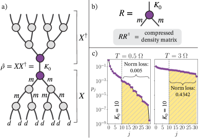
Figure 1: Tree Tensor Operator (TTO) density matrix. (a) A density matrix can be decomposed as $\hat{\rho}=XX^{{\dagger}}$, with columns of $X$ corresponding to $\sqrt{p_{j}}\ket{\psi_{j}}$. In the TTO ansatz, $X$ and $X^{{\dagger}}$ are represented with the tree tensor network-like structures where the connecting link corresponds to the sum over the pure states $\ket{\psi_{j}}$. The bond dimension $m$ corresponds to the bound for system-to-system correlation, and the bond dimension $K_{0}$ is the number of pure states we keep in the density matrix. (b) When isometrized towards the uppermost tensor $R$, the remaining (gray) tensors in a TTO are local unitary transformations. Thus, all the information about bipartite entanglement between the system’s halves is concentrated in the tensor $R$ of controllable dimensions, and its singular values are the square roots of mixed state probabilities $\sqrt{p_{j}}$. (c) Example comparison between thermal probabilities distribution for different temperatures $T$ and the corresponding norm loss after truncating to $K_{0}=10$ lowest-energy states. The norm loss is larger for the higher temperature (right) with respect to the lower temperature (left). The distributions are obtained for a chain of $N=5$ Rydberg atoms ($R_{B}/a=1.14,\Delta/\Omega=2.9$, see Hamiltonian in Eq. (3)).

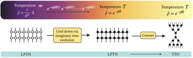
Figure 2: An algorithm for obtaining the thermal density matrix in the TTO form. An infinite-temperature density matrix is always proportional to an identity matrix, and it is therefore straightforward to write in the LPTN form. We take this infinite-temperature density matrix as an initial state and evolve it via the imaginary time evolution, i.e. consecutively applying the operator $e^{-\mathrm{d}\beta\hat{H}/2}$ on both sides of the LPTN. Here, $\mathrm{d}\beta/2$ is an imaginary time step which, in terms of physical interpretation, represents a small decrease in temperature. This way, we can reach a density matrix at an arbitrarily low temperature. Once we reach the desired temperature, we convert the LPTN into the TTO form with the procedure described in Appendix A.

I.2 Obtaining the Tree Tensor Operator density matrix

To access the system’s properties at an arbitrary temperature, we evolve the infinite-temperature density matrix according to the imaginary time evolution Verstraete et al. (2004); Zwolak and Vidal (2004). This is possible due to the fact that an infinite-temperature density matrix, $\hat{\rho}_{\infty}$, is proportional to an identity matrix, allowing to us write:

$$\begin{split}\hat{\rho}&=e^{-\beta\hat{H}}=e^{-\beta\hat{H}/2}\mathds{1}e^{-\beta\hat{H}/2}\\ &\propto e^{-\beta\hat{H}/2}\hat{\rho}_{\infty}e^{-\beta\hat{H}/2}.\end{split}$$ (2)

Therefore, obtaining the density matrix at a certain temperature is mathematically equivalent to performing a time evolution of the identity matrix with an imaginary timestep.

However, we cannot perform imaginary time evolution directly on a TTO: the representation of an identity matrix as a TTO would require the $K_{0}$ dimension to scale exponentially with system size which prohibits the simulation in terms of computational resources. For this reason, we take a deviation via the matrix product state’s mixed state counterpart - the LPTN, which encodes the identity matrix in a trivial way.

We evolve LPTN in imaginary time using the time-dependent variational principle (TDVP) Haegeman et al. (2011, 2016) algorithm. Once we obtain the finite-temperature LPTN density matrix, we convert it to a TTO with an iterative procedure described in Appendix A. The whole procedure for obtaining a TTO thermal density matrix is summarized in Fig. 2.

The timestep we use in imaginary time evolution is $d\beta/2=0.05$ for obtaining the finite temperature phase diagrams in Section III. The value is chosen based on the convergence study, showing that eventual errors are the largest in the vicinity of quantum critical transitions. The value of $d\beta/2$ taken for the analysis at critical regions carried out in Section IV is thus further reduced to $d\beta/2=0.025$. The maximal entanglement bond dimension in LPTN and TTO is $m=50$, and the maximal number of pure states we keep in the TTO density matrix is $K_{0}=100$. The error resulting from truncation in LPTN to TTO conversion is analyzed in Section III.

II Rydberg atom Hamiltonian

We consider a system of two-level Rydberg atoms pinned by optical tweezers. Such system realizes a spin-$1/2$ model by associating the two spin states with the ground state $\ket{g}$ and Rydberg state $\ket{r}$ Browaeys and Lahaye (2020). Rydberg interactions and laser-driven excitations can be encoded through the local Pauli matrix operators $\sigma_{x}=\outerproduct{g}{r}+\outerproduct{r}{g}$ and $n_{z}=\outerproduct{r}{r}$, and in the rotating wave approximation the resulting $N$-site Hamiltonian is:

$$\hat{H} =\frac{\Omega}{2}\sum_{i=1}^{N}\sigma^{i}_{x}-\Delta\sum_{i=1}^{N}n^{i}_{z}+\sum_{i\neq j}\frac{C_{6}}{R_{ij}^{6}}n^{i}_{z}n^{j}_{z},$$ (3)

with indices $i$ and $j$ going over the system sites, $C_{6}$ as the Van der Waals interaction strength, and $R_{ij}$ as the distance between two sites in the lattice. The Rabi frequency $\Omega$ and detuning $\Delta$ are the laser-atom coupling parameters. The units are chosen such that the reduced Planck constant is $\hbar=1$. It is convenient to express the long-range Rydberg interactions in terms of the Rydberg blockade radius per lattice spacing $R_{B}/a$, where $R_{B}=\sqrt[6]{\frac{C_{6}}{\Omega}}$. The blockade radius $R_{B}$ separates a regime in which the interaction is much larger than the Rabi frequency, so the state with more than one excited atom within that radius is shifted far from resonance and thus dynamically decoupled Urban et al. (2009).

We study a chain of $N$ Rydberg atoms described by the Hamiltonian in Eq. (3) with open boundary conditions. In numerical simulations, we set to zero all the interactions that are more than four lattice spacings apart. We choose the lattice spacing $a$ as the unit of length and Rabi frequency $\Omega$ as the unit of energy.

As thoroughly analyzed in the literature, ground states of many-body Rydberg chains are known to exhibit a rich phase diagram Weimer and Büchler (2010); Bernien et al. (2017); Samajdar et al. (2018); Rader and Lauchli (2019); Yu et al. (2022); Maceira et al. (2022). In the regime of small detuning $\Delta/\Omega$, the leading contribution comes from the Rabi term, resulting in a low occupancy of the Rydberg state throughout a system and a disordered phase without any excitation pattern. Increasing the detuning $\Delta/\Omega$, the system starts to favor excitations of the atoms, however, the Rydberg interaction contribution tends to suppress nearby excitations. The interplay between these two contributions results in different excitation patterns, depending on the blockade radius $R_{B}/a$. The emergent phases turn out to be the crystalline phases of $\mathds{Z}_{p}$ symmetry-breaking order (period-$p$), starting from $\mathds{Z}_{2}$ in the low $R_{B}/a$ region, and going towards the higher orders as $R_{B}/a$ increases Bernien et al. (2017); Yu et al. (2022). Accordingly, the transitions between these phases belong to variety of different criticality classes. Moreover, it was shown that the Rydberg phase diagram hosts as well the incommensurate floating phases between disordered and crystalline phases Weimer and Büchler (2010); Rader and Lauchli (2019); Yu et al. (2022); Maceira et al. (2022); Zhang et al. (2024), located in the regions from above the $\mathds{Z}_{3}$ lobe and higher.

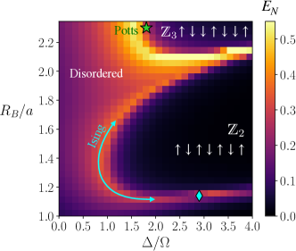
Figure 3: Ground state phase diagram of Rydberg atom Hamiltonian. To detect the phase transition lines of a Rydberg atom Hamiltonian in Eq. (3), we measured the entanglement negativity as the function of the Rydberg blockade radius $R_{B}$ and detuning $\Delta$ for $N=31$ sites at temperature $T=0.025\ \Omega$. The temperature is low enough for the system to approximately be in the ground state (see Section III). We can distinguish two crystalline phases, the ones with $\mathds{Z}_{2}$ and $\mathds{Z}_{3}$ symmetry-breaking order regimes respectively. The transition between the $\mathds{Z}_{2}$ and disordered phase corresponds to the Ising universality class. The green star and blue diamond mark the critical transition points that are analyzed in Section IV, corresponding to the three-state Potts Yu et al. (2022) and Ising universality classes, respectively. Since the position of the marked quantum critical points corresponds to its value in the thermodynamical limit, the line of maximal entanglement is slightly shifted with respect to the Potts critical point position as a consequence of the finite-size effect.

To identify the ground state phases in the parameter range of our simulations, we measure the entanglement negativity $E_{N}$ between two halves of the system at temperature $T=0.025\ \Omega$ in Fig. 3. As shown in the analysis in Section III, this temperature is low enough for the system to be approximately in the ground state. The entanglement negativity is a mixed-state entanglement measure defined as

$$\begin{split}&E_{N}=\frac{\lVert\hat{\rho}^{T_{N/2}}\rVert_{1}-1}{2},\end{split}$$ (4)

where $\hat{\rho}^{T_{N/2}}$ is the partial transpose of $\hat{\rho}$ with respect to half of the system and $\lVert A\rVert_{1}$ is the trace norm, $\lVert A\rVert_{1}=Tr(\sqrt{A^{{\dagger}}A})$. Even though entanglement negativity is constructed as a mixed-state entanglement measure, here we show that it can also be used for quantifying the pure state entanglement, as the phase diagram in Fig. 3 is in line with the existing results obtained via the entanglement entropy Rader and Lauchli (2019); Yu et al. (2022); Maceira et al. (2022). The phase transition lines correspond to maxima in Fig. 3 where one can differentiate three phases in our parameter range: a disordered phase and two crystalline phases. It is known that the transition line between the $\mathds{Z}_{2}$ and disordered phase exhibits the Ising universality behavior. The transition between the $\mathds{Z}_{3}$ and the disordered phase is more complex, and in the parameter range of our simulations, it contains the non-conformal chiral transition line and an isolated point of the three-state Potts universality class.

To avoid edge effects and ensure the non-degeneracy of the ground state in ordered phases, in our simulations, we focus on systems of $6n+1$ sites, which are compatible with non-degenerate configurations both for period-2 and period-3 crystalline orders. In particular, we analyze the systems of $N=13$, $25$, and $31$ sites.

III Finite temperature phase diagrams

In this section, we analyze the thermalized Rydberg systems and assess the resilience of their ground state phases to temperature. For this purpose, we compute the purity

$$\gamma=Tr(\hat{\rho}^{2})=\sum_{j=1}^{K_{0}}p_{j}^{2}$$ (5)

for every point in the phase diagram in Fig. 3 for different temperatures. Since purity can be expressed via the thermal probabilities $p_{j}$, it is straightforward to compute from TTO with a negligible computational cost. In the same way, with TTOs we have access to the global von Neumann entropy and Renyi entropies of any order.

The purity tells us directly about the mixedness of the system; for a pure state, the purity is equal to $1$, and the value decreases as the state becomes more mixed. Therefore, we gain a clear insight into how the ground state turns into a mixture of excited states at finite temperatures (Fig. 4).

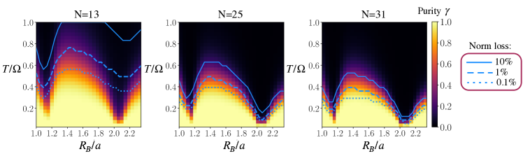
Figure 4: Purity computed for Rydberg atom Hamiltonian. The behavior of the purity with temperature $T$ as the function of Rydberg blockade radius $R_{B}$, computed at $\Delta/\Omega=3.034$, for $N=13$, $25$, $31$ sites. We can observe how the system transitions from the pure ground state at low temperature into the finite-temperature mixture of states. The drops in purity for certain values of $R_{b}/a$ correspond to the points of quantum phase transitions. Moreover, we can clearly see that as the system size increases, the ground state resilience to temperature decreases. The reason why at quantum critical transition points we can observe almost pure state even at finite temperatures is because the system size is finite. Blue curves track the accuracy of the results and denote a temperature above which the norm loss caused by truncation error becomes larger than the certain value indicated in the legend.

The temperature dependence of the purity for different Hamiltonian parameters reflects the structure of the low-energy part of the spectrum. In general, the most important factor deciding on the (non-degenerate) ground state’s resilience to temperature is the energy gap between the ground state and the first excited state, because it directly determines the ratio of the first two largest thermal probabilities, $p_{2}/p_{1}$. Indeed, in the vicinity of quantum critical points in Fig. 4 where the gap decreases (and in thermodynamic limit closes), we can observe the drops in the purity. The fact that at quantum critical transition points we observe a pure state even at finite temperatures is a consequence of finite system size. As we go towards the larger system sizes, the energy levels become more dense and the transition into the finite-temperature mixed phase occurs at lower temperatures.

Recall that the accuracy of our method is limited by the number of excited states we keep in a density matrix, $K_{0}$. This means that, when the state becomes more mixed, the state truncation error becomes larger at fixed $K_{0}$. An easy way of estimating the error induced by discarding the excited states is by tracking the norm loss during the LPTN to TTO conversion. The blue lines in Fig. 4 indicate the temperatures after which the preserved norm falls under a certain factor. As expected, the error increases with the system size for a fixed temperature value. This is because the number of excited states in the spectrum grows exponentially with the system size, and thus, increasing the system size, the number of states $K_{0}$ will represent a smaller ratio of all possible states.

To get an overview of the temperature resilience of ground state phases over the entire phase diagram, we plot the threshold temperature at which the purity falls below a chosen cutoff value, across the entire Hamiltonian parameter range. The obtained finite-temperature phase diagrams for two different values of threshold purity value, $\gamma_{cut}=\{0.5,0.9\}$, are shown in Fig. 5 and one can see that they outline the features of a ground state phase diagram from Fig. 3. The plot minima correspond to the borders between the phases, and the ground state becomes more stable as we go deeper into the crystalline phases. Again, we observe that the transition from the ground state to a mixture of excited states occurs faster for larger systems, i.e. as we go towards the thermodynamic limit.

Since analog quantum simulation experiments often target the ground state, it is instructive to compare our temperature scale to realistic temperature values in Rydberg experiments. The usual experimental Rabi frequency $\Omega$ values are within the MHz range. Taking $\Omega=2.5$ MHz Wurtz et al. (2023), our temperature range $[0.025$, $1]\ \Omega$ from Fig. 5 translates to $[3,\ 120]\ \mu\mathrm{K}$ (or $[0.0625,\ 2.5]$ MHz). Rydberg atom devices usually operate at $\lessapprox 10\ \mu$K ($\simeq 0.2$ MHz) Hölzl et al. (2023); Wurtz et al. (2023), and therefore our results are in line with the fact that the ground state is within the experimental reach for the majority of the Hamiltonian parameter values. However, it should be noted that an experimental system is subject to various additional decoherence effects and motional degrees of freedom, and thus cannot necessarily be considered to be at thermal equilibrium so the temperature of an entire system is not precisely defined. Nevertheless, our results can still provide insight into the ground state resilience on a qualitative level.

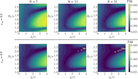
Figure 5: Finite temperature phase diagrams computed for Rydberg atom Hamiltonian. To get an overview of how resilient the ground state ordered phases are to the temperature $T$, we plot the threshold temperature after which the purity $\gamma$ falls below the cutoff value $\gamma_{cut}=0.5$ (up) and $\gamma_{cut}=0.9$ (bottom) as a function of blockade radius $R_{B}/a$ and detuning $\Delta/\Omega$. The results are shown for $N=13$, $25$, $31$ sites. The temperature range is $T=[0.025,\ 1]\ \Omega$. The plots outline the features of the ground phase state diagram, and one can distinguish the $\mathds{Z}_{2}$ and $\mathds{Z}_{3}$ symmetry-breaking phases shrinking as the temperature increases. We can see that, for almost all the Hamiltonian parameter values, the temperature of $T=0.025\ \Omega$ is low enough for purity to be higher than $\gamma_{cut}=0.9$, i.e. for $T=0.025\ \Omega$ we can expect to find the system in the ground state. The exceptions are gray regions in case of $N=25$ and $N=31$ for $\gamma_{cut}=0.9$, located between $\mathds{Z}_{2}$ and $\mathds{Z}_{3}$ lobe, for which our temperature range was not low enough to determine the threshold temperature.

IV Mixed-state entanglement at quantum critical points

In this section, we focus on the conformal phase transition points. In particular, we compute the mixed-state entanglement monotones at two points belonging to the Ising universality class and the Potts universality class Yu et al. (2022) (marked with a blue diamond and a green star in Fig. 3). Exploiting the TTO ansatz, we measure the temperature dependence of the bipartite entanglement between the two halves of the system via two mixed-state entanglement measures: the entanglement negativity defined in Eq. (4), and the entanglement of formation. The entanglement of formation is the mixed-state generalization of entanglement entropy. Mathematically, it is defined as a weighted sum of entanglement entropies minimized over all the possible pure-state decompositions of $\hat{\rho}$, and is defined as:

$$\begin{split}&E_{F}=\inf_{\psi_{j},p_{j}}\Bigl{\{}\sum_{j}p_{j}\mathcal{S}_{E}(\ket{\psi_{j}})\ \ :\ \ \hat{\rho}=\sum_{j}p_{j}\ket{\psi_{j}}\bra{\psi_{j}}\Bigr{\}},\\ \end{split}$$ (6)

with $\mathcal{S}_{E}$ denoting the entanglement entropy of half-system bipartition. In general, calculating the entanglement of formation is an extremely challenging task, and exact solutions are known only for small system sizes Hill and Wootters (1997); Wootters (1998) or very specific cases Terhal and Vollbrecht (2000); Vollbrecht and Werner (2001).

Here, we compute it using the procedure presented in Arceci et al. (2021), improved as described in Appendix B. In order to improve the convergence of the results, we truncate the $K_{0}$ dimension even further and keep the first $K_{0}=10$ states in the density matrix for the computation of entanglement of formation. Note that, as discussed in Section III, reducing the number of states in the density matrix increases the error in the high-temperature region. Therefore, we carry out the entanglement of formation analysis only in the low-temperature region in which the norm loss is smaller than $1\%$.

The results for Ising and Potts quantum critical points are plotted in Fig. 6. From both entanglement measures, we observe that entanglement is approximately constant up to a certain temperature, after which it starts to decrease. Following the analysis from Section III, the temperature region in which the entanglement is constant corresponds to the temperature region in which the state remains approximately pure.

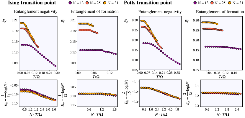
Figure 6: Thermal state entanglement at quantum critical points. Finite-temperature decay and scaling of entanglement negativity $E_{N}$ and entanglement of formation $E_{F}$ in the vicinity of the Ising critical point at $R_{B}/a=1.142$, $\Delta/\Omega=2.9$ (left) and the Potts critical point at $R_{B}/a=2.3$, $\Delta/\Omega=1.808$ Yu et al. (2022) (right), computed for $N=13$, $25$, and $31$ sites. The insets show the entanglement curves after rescaling according to Eq. (7). The curves show a good agreement in scaling with respect to the order of magnitude of entanglement values. The shape of the rescaled curves correspond to the functions $g_{N}(\cdot)$ and $g_{F}(\cdot)$ from Eq. (7).

The next step is to analyze and quantify finite-size effects, i.e. how entanglement scales with system size and temperature. The numerical results on the entanglement of formation $E_{F}$ in low-temperature Ising and Luttinger liquid XXZ model Arceci et al. (2021) predicted that in the vicinity of the conformal quantum critical point, $E_{F}$ should follow the logarithmic scaling. This scaling relation is the finite-temperature extension of the conformal field theory scaling for entanglement entropy. For open boundary conditions, central charge $c$, and dynamical critical exponent $z$ it reads:

$$\begin{split}&E_{F}(T,N)=\frac{c}{6}\mathrm{log}(N)+g_{F}(TN^{z}),\end{split}$$ (7)

where $g_{F}(\cdot)$ is a function depending on the model characteristics. Here, we neglect the corrections coming from the odd number of sites and the unequal length of the two system halves. We check if the same scaling holds in our Hamiltonian in the vicinity of the Ising and the three-state Potts transition point when the correct exponents are used ($c=1/2$, $z=1$ for Ising and $c=4/5$, $z=1$ for Potts). Moreover, we check if the analogous scaling is valid as well for entanglement negativity. Rescaling both entanglement measure curves, the results in Fig. 6 show a good agreement with Eq. (7). The slight discrepancy in the scaling of $N=13$ entanglement negativity at the Ising critical point is most likely due to the finite system size. Altogether, Eq. (7) represents a tool for estimating the many-body mixed-state entanglement measures in the low-temperature region of conformal critical points, based on the results for small system size.

V Conclusions

We have presented a tensor network algorithm for obtaining a thermal many-body density matrix and exploited our approach to study the finite-temperature effects on one-dimensional Rydberg atom systems of up to 31 particles. By computing the purity for different Hamiltonian parameters, we have studied the transition from the low-temperature pure state to the finite-temperature mixed state and demonstrated how the system’s response to the temperature depends strongly on the structure of the low-energy part of the spectrum. Indeed, the transition from the gapped to the gapless point in the phase diagram is characterized by sudden drops in the property’s resilience to the temperature. By plotting the temperature resilience of the system’s purity over the Hamiltonian parameters, we have identified the crystalline $\mathds{Z}_{2}$ and $\mathds{Z}_{3}$ - symmetry-breaking phases and clearly observed how they shrink when increasing the temperature. We have recognized the ground state phase transition curves as the curves where the system’s properties are the most sensitive to temperature. Moreover, as expected, larger systems have shown higher sensitivity to temperature effects in comparison to smaller systems.

The Rydberg chain ground state phase diagram hosts a variety of different criticality classes, and we have analyzed the temperature effects on the entanglement at the Ising and the three-state Potts quantum critical points using the mixed-state entanglement monotones negativity and entanglement of formation. Both monotones have shown the same behavior where entanglement stays unaltered up to a certain temperature and then decreases towards higher temperatures. By performing a finite-size scaling analysis of both entanglement monotones, we have provided numerical evidence that the entanglement scaling law at conformal critical points extends from the zero temperature point to the low-temperature region. Therefore, this scaling law can be used to estimate the many-body mixed-state entanglement for large system sizes, based on the results obtained for a small system size.

Overall, we have stressed that addressing finite temperature equilibrium problems requires dedicated algorithms. From a computational perspective, simulating finite-temperature, i.e. mixed many-body quantum states, represents an additional difficulty in comparison to the already computationally demanding zero-temperature quantum many-body simulations. Our algorithm represents an efficient way of obtaining the density matrix and provides adaptability to convert from LPTN geometry, suitable for imaginary time evolution, to TTO geometry, suitable for characterization of the mixed state properties. The procedure is flexible to use beyond Rydberg systems and therefore can be employed as a toolbox for studying finite temperature physics of a general quantum many-body model.

Data and code availability

The simulations were performed using the Quantum Green Tea software version 0.3.23 and Quantum Tea Leaves version 0.4.46 Ballarin et al. (2024). All the simulation scripts, full datasets, and metadata are available on Zenodo Reinić et al. (2024a), and all the figures are available at Reinić et al. (2024b).

Appendix A LPTN to TTO conversion

Here, we explain the algorithm for converting the LPTN density matrix into TTO form. Since both LPTN and TTO contain two sides of the network that are Hermitian conjugated to each other, referred to as $X$ and $X^{{\dagger}}$ in Fig. 1, it is enough to discard one of them and perform all the computations on only one of the sides. The procedure follows the steps in Fig. 7. Starting from the $N$-site LPTN, where $N=2^{n}$, $n$ being an integer, we first contract pairs of tensors (Fig. 7a). Then, we apply a truncated singular value decomposition (SVD) to the obtained tensors over a bipartition of links as indicated with purple dashed lines in Fig. 7b. The singular values are contracted to the upper tensors, and the lower tensors will remain unitary with respect to the corresponding bipartition of links. These lower tensors represent the log($N$)-th layer of the TTO. To create a base for building the next layer, we again apply a truncated SVD to the yellow tensors according to the specified bipartition (Fig. 7c), and this time contract the singular values to the lower tensors. In this case, the upper tensors stay unitary. Since the total density matrix contains as well the Hermitian conjugate part contracted over the upper bonds, we can ignore these upper unitary tensors because they contract with their Hermitian conjugates to an identity (Fig. 7d). We obtain the tensor network form as in Fig. 7e. The upper layer of tensors in Fig. 7e has the LPTN-like form of half as many particles. Therefore, we can iterate the described procedure to build the rest of the TTO layers. Notice that this procedure by its construction guarantees that the isometry center is installed to the uppermost tensor. Moreover, to increase the accuracy of our method we make sure that at each singular value truncation, the isometry center of LPTN is placed at that tensor.

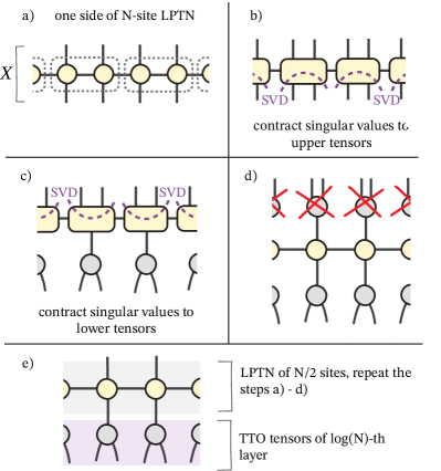
Figure 7: Conversion from Locally Purified Tensor Network to Tree Tensor Operator. Black dotted rectangles denote the contraction of the enclosed tensors. The purple dashed line defines the bipartition of links for singular value decomposition (SVD). Moreover, the gray color of a tensor denotes that the tensor is unitary with respect to the appropriate bipartition of links defined by the preceding SVD.

As noted above, TTOs are compatible only with the number of sites that are powers of two, however, the system sizes needed to realize the period-2 and period-3 phases in the Rydberg phase diagram are not powers of two. To overcome this issue, we run the imaginary time evolution on the odd-sited LPTN, and then insert the dummy sites decoupled from the rest of the system on the LPTN’s edges. This way, the sites are artificially padded on both ends of the LPTN such that the new total number of sites is a power of two, without affecting any of the properties that we measure.

Appendix B Entanglement of formation minimization

To minimize entanglement of formation in Eq. (6), we need to find the optimal pure state decomposition of the density matrix. As explained in Ref. Arceci et al. (2021), a certain pure state decomposition of a density matrix is parametrized by a unitary matrix applied to TTO’s uppermost tensor. Therefore, the optimization time depends heavily on how we sample the unitary matrices.

Here, we improve the method proposed in Ref. Arceci et al. (2021), which relied on constructing the unitary matrix as an exponential of the Hermitian matrix. The drawback of such an approach is that a small change in a parameter of the Hermitian matrix can, in general, result in a large change in the elements of the corresponding unitary matrix.

We solve this issue by using the Nelder-Mead algorithm, which is a simplex-based optimization method. We construct each point of the simplex by multiplying the initial guess for the unitary matrix with squashed Haar-random unitary matrices, defined as

$$\begin{split}&U_{\mathrm{squash}}=U^{\dagger}D^{\alpha}U,\end{split}$$ (8)

where $U_{\mathrm{Haar}}=U^{\dagger}DU$ is an eigenvalue decomposition of the Haar-random unitary matrix Mezzadri (2007), and $\alpha\in[0,1]$. This way, we ensure that in every iteration of the search algorithm, the elements of a new guess for the unitary matrix are arbitrarily close to the elements of a previous guess, controlled with the parameter $\alpha$.

Moreover, using physical intuition we can pick a convenient initial guess for the unitary matrix based on the following reasoning. The properties of the density matrix change continuously with increasing temperature. Therefore, if we run the entanglement of formation computation for temperature points starting from the lowest temperature, we can choose the initial guess of every new point to be the optimized unitary matrix from a previous point. Such a choice additionally speeds up the computation.

References

- Urban et al. (2009) E. Urban, T. A. Johnson, T. Henage, L. Isenhower, D. D. Yavuz, T. G. Walker, and M. Saffman, “Observation of Rydberg blockade between two atoms,” Nature Physics 5, 110–114 (2009).
- Löw et al. (2012) Robert Löw, Hendrik Weimer, Johannes Nipper, Jonathan B. Balewski, Björn Butscher, Hans Peter Büchler, and Tilman Pfau, “An experimental and theoretical guide to strongly interacting Rydberg gases,” J. Phys. B: At. Mol. Opt. Phys. 45 (2012).
- Weber et al. (2017) Sebastian Weber, Christoph Tresp, Henri Menke, Alban Urvoy, Ofer Firstenberg, Hans Peter Büchler, and Sebastian Hofferberth, “Calculation of Rydberg interaction potentials,” J. Phys. B: At. Mol. Opt. Phys. 50 (2017).
- Wu et al. (2021) Xiaoling Wu, Xinhui Liang, Yaoqi Tian, Fan Yang, Cheng Chen, Yong-Chun Liu, Meng Khoon Tey, and Li You, “A concise review of Rydberg atom based quantum computation and quantum simulation,” Chinese Physics B 30 (2021).
- Browaeys and Lahaye (2020) Antoine Browaeys and Thierry Lahaye, “Many-body physics with individually controlled Rydberg atoms,” Nature Physics 16, 132–142 (2020).
- Kaufman and Ni (2021) Adam M. Kaufman and Kang-Kuen Ni, “Quantum science with optical tweezer arrays of ultracold atoms and molecules,” Nature Physics 17, 1324–1333 (2021).
- Barredo et al. (2018) Daniel Barredo, Vincent Lienhard, Sylvain de Léséleuc, Thierry Lahaye, and Antoine Browaeys, “Synthetic three-dimensional atomic structures assembled atom by atom,” Nature 561, 79–82 (2018).
- Endres et al. (2016) Manuel Endres, Hannes Bernien, Alexander Keesling, Harry Levine, Eric R. Anschuetz, Alexandre Krajenbrink, Crystal Senko, Vladan Vuletic, Markus Greiner, and Mikhail D. Lukin, “Atom-by-atom assembly of defect-free one-dimensional cold atom arrays,” Science 354, 1024–1027 (2016).
- Manetsch et al. (2024) Hannah J. Manetsch, Gyohei Nomura, Elie Bataille, Kon H. Leung, Xudong Lv, and Manuel Endres, “A tweezer array with 6100 highly coherent atomic qubits,” arXiv preprint (2024).
- Levine et al. (2019) Harry Levine, Alexander Keesling, Giulia Semeghini, Ahmed Omran, Tout T. Wang, Sepehr Ebadi, Hannes Bernien, Markus Greiner, Vladan Vuletić, Hannes Pichler, and Mikhail D. Lukin, “Parallel implementation of high-fidelity multiqubit gates with neutral atoms,” Nature 123 (2019).
- Zhuo et al. (2022) Fu Zhuo, Xu Peng, Sun Yuan, Liu Yang-Yang, He Xiao-Dong, Li Xiao, Liu Min, Li Run-Bing, Wang Jin, Liu Liang, , and Zhan Ming-Sheng, “High-fidelity entanglement of neutral atoms via a Rydberg-mediated single-modulated-pulse controlled-phase gate,” Phys. Rev. A 105 (2022).
- Evered et al. (2023) Simon J. Evered, Dolev Bluvstein, Marcin Kalinowski, Sepehr Ebadi, Tom Manovitz, Hengyun Zhou, Sophie H. Li, Alexandra A. Geim, Tout T. Wang, Nishad Maskara, Harry Levine, Giulia Semeghini, Markus Greiner, Vladan Vuletić, and Mikhail D. Lukin, “High-fidelity parallel entangling gates on a neutral-atom quantum computer,” Nature 622, 268–272 (2023).
- Bluvstein et al. (2022) Dolev Bluvstein, Harry Levine, Giulia Semeghini, Tout T. Wang, Sepehr Ebadi, Marcin Kalinowski, Alexander Keesling, Nishad Maskara, Hannes Pichler, Markus Greiner, Vladan Vuletić, and Mikhail D. Lukin, “A quantum processor based on coherent transport of entangled atom arrays,” Nature 604, 451–456 (2022).
- Bluvstein et al. (2023) Dolev Bluvstein, Simon J. Evered, Alexandra A. Geim, Sophie H. Li, Hengyun Zhou, Tom Manovitz, Sepehr Ebadi, Madelyn Cain, Marcin Kalinowski, Dominik Hangleiter, J. Pablo Bonilla Ataides, Nishad Maskara, Iris Cong, Xun Gao, Pedro Sales Rodriguez, Thomas Karolyshyn, Giulia Semeghini, Michael J. Gullans, Markus Greiner, Vladan Vuletić, and Mikhail D. Lukin, “Logical quantum processor based on reconfigurable atom arrays,” Nature 626, 58–65 (2023).
- Gross and Bloch (2017) Christian Gross and Immanuel Bloch, “Quantum simulations with ultracold atoms in optical lattices,” Science 357, 995–1001 (2017).
- Wurtz et al. (2023) Jonathan Wurtz, Alexei Bylinskii, Boris Braverman, Jesse Amato-Grill, Sergio H. Cantu, Florian Huber, Alexander Lukin, Fangli Liu, Phillip Weinberg, John Long, Sheng-Tao Wang, Nathan Gemelke, and Alexander Keesling, “Aquila: Quera’s 256-qubit neutral-atom quantum computer,” arXiv preprint (2023).
- Bernien et al. (2017) H. Bernien, S. Schwartz, A. Keesling, H. Levine, A. Omran, H. Pichler, S. Choi, A. S. Zibrov, M. En. M. Greiner, V. Vuletić, and M. D. Lukin, “Probing many-body dynamics on a 51-atom quantum simulator,” Nature 551, 579–584 (2017).
- Keesling et al. (2019) A. Keesling, A. Omran, H. Levine, H. Bernien, H. Pichler, S. Choi, R. Samajdar, S. Schwartz, P. Silvi, S. Sachdev, P. Zoller, M. Endres, M. Greiner, V. Vuletić, and M. D. Lukin, “Quantum Kibble–Zurek mechanism and critical dynamics on a programmable Rydberg simulator,” Nature 568, 207–211 (2019).
- De Léséleuc et al. (2019) Sylvain De Léséleuc, Vincent Lienhard, Pascal Scholl, Daniel Barredo, Sebastian Weber, Nicolai Lang, Hans Peter Büchler, Thierry Lahaye, and Antoine Browaeys, “Observation of a symmetry-protected topological phase of interacting bosons with Rydberg atoms,” Science 365, 775–780 (2019).
- Scholl et al. (2021) Pascal Scholl, Michael Schuler, Hannah J. Williams, Alexander A. Eberharter, Daniel Barredo, Kai-Niklas Schymik, Vincent Lienhard, Louis-Paul Henry, Thomas C. Lang, Thierry Lahaye, Andreas M. Läuchli, and Antoine Browaeys, “Quantum simulation of 2d antiferromagnets with hundreds of Rydberg atoms,” Nature 595, 233–238 (2021).
- Ebadi et al. (2021) Sepehr Ebadi, Tout T. Wang, Harry Levine, Alexander Keesling, Giulia Semeghini, Ahmed Omran, Dolev Bluvstein, Rhine Samajdar, Hannes Pichler, Wen Wei Ho, Soonwon Choi, Subir Sachdev, Markus Greiner, Vladan Vuletić, and Mikhail D. Lukin, “Quantum phases of matter on a 256-atom programmable quantum simulator,” Nature 595, 227–232 (2021).
- Zhang et al. (2024) Jin Zhang, Sergio H. Cantú, Fangli Liu, Alexei Bylinskii, Boris Braverman, Florian Huber, Jesse Amato-Grill, Alexander Lukin, Nathan Gemelke, Alexander Keesling, Sheng-Tao Wang, Y. Meurice, and S.-W. Tsai, “Probing quantum floating phases in Rydberg atom arrays,” arXiv preprint 2401.08087 (2024).
- Amico et al. (2008) Luigi Amico, Rosario Fazio, Andreas Osterloh, and Vlatko Vedral, “Entanglement in many-body systems,” Rev. Mod. Phys. 80 (2008).
- Baccari et al. (2017) Flavio Baccari, Daniel Cavalcanti, Peter Wittek, and Antonio Acín, “Efficient device-independent entanglement detection for multipartite systems,” Phys. Rev. X 7 (2017).
- Friis et al. (2018) Nicolai Friis, Giuseppe Vitagliano, Mehul Malik, and Huber Marcus, “Entanglement certification from theory to experiment,” Nature Reviews Physics 1, 72–87 (2018).
- Daley et al. (2012) Andrew J. Daley, Hannes Pichler, Johannes Schachenmayer, and Peter Zoller, “Measuring entanglement growth in quench dynamics of bosons in an optical lattice,” Phys. Rev. Lett. 109 (2012).
- Islam et al. (2015) Rajibul Islam, Ruichao Ma, Philipp M. Preiss, M. Eric Tai, Alexander Lukin, Matthew Rispoli, and Markus Greiner, “Measuring entanglement entropy in a quantum many-body system,” Nature 528, 77–83 (2015).
- Elben et al. (2023) Andreas Elben, Steven T. Flammia, Hsin-Yuan Huang, Richard Kueng, John Preskill, Benoît Vermersch, and Peter Zoller, “The randomized measurement toolbox,” Nature Reviews Physics 5, 9–24 (2023).
- Notarnicola et al. (2023) Simone Notarnicola, Andreas Elben, Thierry Lahaye, Antoine Browaeys, Simone Montangero, and Benoît Vermersch, “A randomized measurement toolbox for an interacting Rydberg-atom quantum simulator,” New Journal of Physics 25 (2023).
- Elben et al. (2020) Andreas Elben, Richard Kueng, Hsin-Yuan (Robert) Huang, Rick van Bijnen, Christian Kokail, Marcello Dalmonte, Pasquale Calabrese, Barbara Kraus, John Preskill, Peter Zoller, and Benoît Vermersch, “Mixed-state entanglement from local randomized measurements,” Phys. Rev. Lett. 125 (2020).
- Eisert et al. (2010) J. Eisert, M. Cramer, and M. B. Plenio, “Colloquium: Area laws for the entanglement entropy,” Rev. Mod. Phys. 82 (2010).
- Laflorencie (2016) Nicolas Laflorencie, “Quantum entanglement in condensed matter systems,” Rev. Mod. Phys. 646, 1–59 (2016).
- Bennett et al. (1996a) Charles H. Bennett, Herbert J. Bernstein, Sandu Popescu, and Benjamin Schumacher, “Concentrating partial entanglement by local operations,” Phys. Rev. A 53 (1996a).
- Cui et al. (2013) Jian Cui, Luigi Amico, Heng Fan, Mile Gu, Alioscia Hamma, and Vlatko Vedral, “Local characterization of one-dimensional topologically ordered states,” Phys. Rev. B 88 (2013).
- Bruß (2002) Dagmar Bruß, “Characterizing entanglement,” J. Math. Phys. 43, 4237–4251 (2002).
- Plenio and Virmani (2007) Martin B. Plenio and Shashank Virmani, “An introduction to entanglement measures,” Quant. Inf. Comput. 7, 1–51 (2007).
- Bennett et al. (1996b) Charles H. Bennett, David P. DiVincenzo, John A. Smolin, and William K. Wootters, “Mixed-state entanglement and quantum error correction,” Phys. Rev. A 54 (1996b).
- Arceci et al. (2021) L. Arceci, P. Silvi, and S. Montangero, “Entanglement of formation of mixed many-body quantum states via tree tensor networks,” Phys. Rev. Lett. 128 (2021).
- Werner et al. (2016) A. H. Werner, D. Jaschke, P. Silvi, M. Kliesch, T. Calarco, J. Eisert, and Montangero S., “Positive tensor network approach for simulating open quantum many-body systems,” Phys. Rev. Lett. 116 (2016).
- Schollwöck (2011) Ulrich Schollwöck, “The density-matrix renormalization group in the age of matrix product states,” Annals of Physics 326, 96–192 (2011).
- Vidal and Werner (2002) G. Vidal and R. F. Werner, “Computable measure of entanglement,” Phys. Rev. A 65 (2002).
- Wichterich et al. (2010) Hannu Wichterich, Julien Vidal, and Sougato Bose, “Universality of the negativity in the Lipkin-Meshkov-Glick model,” Phys. Rev. A 81 (2010).
- Calabrese et al. (2014) Pasquale Calabrese, John Cardy, and Erik Tonni, “Finite temperature entanglement negativity in conformal field theory,” J. Phys. A: Math. Theor. 48 (2014).
- Silvi et al. (2019) P. Silvi, F. Tschirsich, M. Gerster, J. Jünemann, D. Jaschke, M. Rizzi, and S. Montangero, “The tensor networks anthology: Simulation techniques for many-body quantum lattice systems,” SciPost Phys. Lect. Notes 8 (2019).
- Verstraete et al. (2004) F. Verstraete, J. J. García-Ripoll, and J. I. Cirac, “Matrix product density operators: Simulation of finite-temperature and dissipative systems,” Phys. Rev. Lett. 93 (2004).
- Zwolak and Vidal (2004) Michael Zwolak and Guifré Vidal, “Mixed-state dynamics in one-dimensional quantum lattice systems: A time-dependent superoperator renormalization algorithm,” Phys. Rev. Lett. 93, 207205 (2004).
- Haegeman et al. (2011) Jutho Haegeman, J. Ignacio Cirac, Tobias J. Osborne, Iztok Pižorn, Henri Verschelde, and Frank Verstraete, “Time-dependent variational principle for quantum lattices,” Phys. Rev. Lett. 107 (2011).
- Haegeman et al. (2016) Jutho Haegeman, Christian Lubich, Ivan Oseledets, Bart Vandereycken, and Verstraete Frank, “Unifying time evolution and optimization with matrix product states,” Phys. Rev. B 94 (2016).
- Weimer and Büchler (2010) Hendrik Weimer and Hans Peter Büchler, “Two-stage melting in systems of strongly interacting Rydberg atoms,” Phys. Rev. Lett. 105 (2010).
- Samajdar et al. (2018) Rhine Samajdar, Soonwon Choi, Hannes Pichler, Mikhail D. Lukin, and Subir Sachdev, “Numerical study of the chiral quantum phase transition in one spatial dimension,” Phys. Rev. A 98 (2018).
- Rader and Lauchli (2019) M. Rader and A. M. Lauchli, “Floating phases in one-dimensional Rydberg Ising chains,” arXiv preprint 1908.02068 (2019).
- Yu et al. (2022) X. Yu, S. Yang, J. Xu, and L. Xu, “Fidelity susceptibility as a diagnostic of the commensurate-incommensurate transition: A revisit of the programmable Rydberg chain,” Phys. Rev. B 106 (2022).
- Maceira et al. (2022) Ivo A. Maceira, Natalia Chepiga, and Frédéric Mila, “Conformal and chiral phase transitions in Rydberg chains,” Phys. Rev. Research 4 (2022).
- Hölzl et al. (2023) C. Hölzl, A. Götzelmann, M. Wirth, M. S. Safronova, S. Weber, and F. Meinert, “Motional ground-state cooling of single atoms in state-dependent optical tweezers,” Phys. Rev. Research 5 (2023).
- Hill and Wootters (1997) S. A. Hill and W. K. Wootters, “Entanglement of a pair of quantum bits,” Phys. Rev. Lett. 78 (1997).
- Wootters (1998) W. K. Wootters, “Entanglement of formation of an arbitrary state of two qubits,” Phys. Rev. Lett. 80 (1998).
- Terhal and Vollbrecht (2000) Barbara M. Terhal and Karl Gerd H. Vollbrecht, “Entanglement of formation for isotropic states,” Phys. Rev. Lett. 85 (2000).
- Vollbrecht and Werner (2001) K. G. H. Vollbrecht and R. F. Werner, “Entanglement measures under symmetry,” Phys. Rev. A 64 (2001).
- Ballarin et al. (2024) Marco Ballarin, Giovanni Cataldi, Aurora Costantini, Daniel Jaschke, Giuseppe Magnifico, Simone Montangero, Simone Notarnicola, Alice Pagano, Luka Pavesic, Marco Rigobello, Nora Reinić, Simone Scarlatella, and Pietro Silvi, “Quantum TEA: qtealeaves,” (2024).
- Reinić et al. (2024a) Nora Reinić, Daniel Jaschke, Darvin Wanisch, Pietro Silvi, and Simone Montangero, “Simulation scripts for "Finite-temperature Rydberg arrays: quantum phases and entanglement characterization",” (2024a).
- Reinić et al. (2024b) Nora Reinić, Daniel Jaschke, Darvin Wanisch, Pietro Silvi, and Simone Montangero, “Figures for "Finite-temperature Rydberg arrays: quantum phases and entanglement characterization",” (2024b).
- Mezzadri (2007) Francesco Mezzadri, “How to generate random matrices from the classical compact groups,” Notices of the American Mathematical Society 54, 592–604 (2007).