Classifying Overlapping Gaussian Mixtures in High Dimensions: From Optimal Classifiers to Neural Nets
Abstract
We derive closed-form expressions for the Bayes optimal decision boundaries in binary classification of high dimensional overlapping Gaussian mixture model (GMM) data, and show how they depend on the eigenstructure of the class covariances, for particularly interesting structured data. We empirically demonstrate, through experiments on synthetic GMMs inspired by real-world data, that deep neural networks trained for classification, learn predictors which approximate the derived optimal classifiers. We further extend our study to networks trained on authentic data, observing that decision thresholds correlate with the covariance eigenvectors rather than the eigenvalues, mirroring our GMM analysis. This provides theoretical insights regarding neural networks’ ability to perform probabilistic inference and distill statistical patterns from intricate distributions.
1 Introduction
There is a well-accepted understanding in machine learning that inherent correlations or statistical structure within the data play a crucial role in enabling effective modeling. The presence of structure in the data provides important context that machine learning algorithms can leverage for accurate and meaningful knowledge extraction and generalization. Harnessing any inherent structure is widely seen as an important factor for achieving successful learning outcomes.
Determining the characteristics of natural datasets that contribute to effective training and good generalization has tremendous theoretical and practical significance. Regrettably, real-world datasets are typically viewed as samples drawn from some unknown, intricate, high-dimensional underlying population, rendering analyses that depend on accurately modeling the true distribution enormously challenging. Connecting properties of the data to learning outcomes is difficult because real data does not readily yield its generative process or population distribution.
While fully characterizing natural data distributions remains difficult, progress can still be made by considering simplified models that capture key aspects of the true distribution. One approach is to model the data via the moment expansion of the underlying population. For a random vector representing a single sample, its distribution can be described by the moment generating function . Approximating this by retaining a finite number of moments provides a tractable model of the data distribution.
A simple starting point is the Gaussian model, which posits that a dataset’s statistical properties can be fully captured by its first two moments - the mean vector and sample covariance matrix. This assumes higher-order dependencies are negligible such that the distribution is characterized solely by its first and second central statistical moments.
In the last decade, analyzing the behavior of machine learning algorithms on idealized i.i.d. Gaussian datasets has emerged as an important area of research in high-dimensional statistics (Donoho and Tanner, 2009; Korada and Montanari, 2011; Monajemi et al., 2013; Candès et al., 2020; Bartlett et al., 2020). Studying these simplified synthetic distributions has provided valuable insights, such as neural network scaling laws (Maloney et al., 2022; Kaplan et al., 2020), universal convergence properties (Seddik et al., 2020) and an improved understanding of the "Double Descent" phenomenon (Montanari and Saeed, 2022). Examining learning on Gaussian approximations of real data distributions has helped establish foundational understandings of algorithmic behavior in high-dimensional settings.
A particular case of interest is that of data which is divided into a set number of classes. In certain instances, the data can be described by a mixture model, where each sample is generated separately for each class. The simplest example of such distributions is that of a Gaussian Mixture Model (GMM), on which we focus in this work.
Gaussian mixtures are a popular model in high-dimensional statistics since, besides being an universal approximator, they often lead to mathematically tractable problems. Indeed, a recent line of work has analyzed the asymptotic performance of a large class of machine learning problems in the proportional high-dimensional limit under the Gaussian mixture data assumption, see e.g. Mai and Liao (2019); Mignacco et al. (2020a); Taheri et al. (2020); Kini and Thrampoulidis (2021); Wang and Thrampoulidis (2021); Refinetti et al. (2021); Loureiro et al. (2021a).
In light of the insights gained by studying the unsupervised, perspective on GMM classification, we focus here on a complementary direction. Namely, we consider the supervised setting, where a single neural network is trained on a dataset generated from a GMM, to perform binary classification where the true labels are given. To connect the GMM with real-world data, we restrict ourselves to the case of strictly non-linearly separable GMMs, such that the class means difference is negligible compared to the class covariance difference. We refer to this setup as overlapping GMM classification.
Our main contributions are as follows:
-
•
In Section 3, we derive the Bayes Optimal Classifiers (BOCs) and decision boundaries for overlapping GMM classification problems, both in the population and the empirical limits.
-
•
In Section 4, under the assumptions of correlated features and Haar distributed eigenvectors, we are able to provide approximate closed form equations for the decision boundaries and discriminator distributions, as a function of the eigenvalues and eigenvectors of the different class covariances.
-
•
In Section 5, we present empirical evidence, demonstrating that some networks trained to perform binary classification on a GMM, approximate the BOC. We further relate these observations to existing results, namely convergence of homogeneous networks to a KKT point.
-
•
In Section 6, we demonstrate empirically that for high dimensional data, the covariance eigenvectors and not the eigenvalues determine the classification threshold for deep neural networks trained on real-world datasets, and provide an explanation inspired by our results on GMMs. In Section 7 we summarize our conclusions and outlook.
2 Background and Related Work
There has been significant work aimed at understanding the classification capabilities of Gaussian mixture models (GMMs), that is, recovering the cluster label for each data point rather than using labels provided by a teacher. For binary classification problems, examples include methods proposed by Mai et al. (2019), Mignacco et al. (2020b), and Deng et al. (2022), with the latter also demonstrating an equivalence between classification and single-index models. In multi-class settings, (Thrampoulidis et al., 2020) analyzed the performance of ridge regression classifiers. The most general results in this area are from Gaussian Mix Group (Loureiro et al., 2021b), which considers the use of GMMs with any convex loss function for classification. Additional results regarding kernels and GMMs include (Couillet et al., 2018; Liao and Couillet, 2019; Kammoun and Couillet, 2023; Refinetti et al., 2021), precise asymptotics (Loureiro et al., 2021c) and the connection between GMMs and real-world vision data (Ingrosso and Goldt, 2022). Additionally, work has been done to understand Quadratic Discriminant Analysis (QDA) in high dimensions (Elkhalil et al., 2017; Ghojogh and Crowley, 2019; Das and Geisler, 2021), which we rely heavily upon in this work.
3 Overlapping Gaussian Mixtures in High Dimensions
Consider the task of performing binary classification on samples drawn from a two class GMM, where the underlying Gaussian distributions have similar means but different covariance matrices. We generate two datasets of equal size , and the same data dimensions . Here, each sample vector is drawn from a jointly normal distribution, either or , where the two means and covariance matrices distinguish between the two classes. In this setup, we assign a label value to samples drawn from class and for the class samples. Throughout this work, we consider the large number of features and large number of samples limit , while the ratio is constant. We denote as the population limit, while as the empirical limit.
In the following sections, we discuss the optimal classifiers obtained first from the population and then the empirical data distributions. We then apply our results to a simplified model dataset which captures some of the properties of real-world datasets, and distinguish the roles of the covariance eigenvectors and eigenvalues for this case.
3.1 Optimal Classification on Population Data
The Bayes-optimal classifier (BOC) assigns each sample to the class that maximizes the expected value gain or its logarithm defined as
| (1) |
where is the class density with the number of classes in the case of a balanced dataset. Here, is the conditional in-class density. The decision boundary between any two classes is given when , where the probabilities of a sample being classified as or are equal. For a two-class GMM, this is obtained by simply equating the class conditional probability densities, i.e., , leading to the quadratic decision rule, derived in Elkhalil et al. (2017) as well as Das and Geisler (2021), to pick class if
| (2) | ||||
where is the determinant of the matrix . This quadratic is the Bayes classifier, or the Bayes decision variable that, when compared to zero, maximizes expected gain.
Note that the term in Equation 2 determines the linear decision boundary, while determines the nonlinear part. For the rest of this work, we consider the nonlinear, overlapping mixture configuration, where , while , as a proxy for the behavior of many real world datasets (Schilling et al., 2021). Without loss of generality, we may set , since we can always shift away the mean of the distributions, resulting in the simpler form of
| (3) |
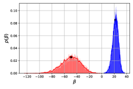
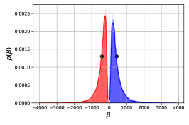
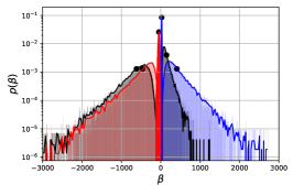
where the last transition in Equation 3 is valid since is given by a sum of distributed random variables, known as the generalized chi-squared distribution (Das and Geisler, 2021), where , are the eigenvalues of , and . The probability density function (PDF) of does not have a closed analytic form, but can be obtained numerically by various methods (Ferrari, 2019; Das and Geisler, 2021). In Figure 1, we show the -distribution for high-dimensional Gaussian data with different covariances, obtained both empirically from Equation 3 and by drawing from a sum of variables matching Equation 3.
While the full PDF of cannot be written in a simple form, the empirical expectation value on a given set of measurements can be derived. Namely, given a set of samples , taken from a normal distribution , the expectation value of the Bayes classifier on these samples is simply
| (4) |
where indicates averaging over the data distribution. It can be used to define what it means for a sample to belong to class or , by computing the average distance between the expectation value of on any dataset and the class values, given by
| (5) |
where we averaged over samples from the distributions, and . We show these values as black dots in Figure 1.
3.2 Empirical Optimal Classification
So far, we have assumed that we have access to the population covariances . Here, we comment on the classification problem changes when relaxing this assumption and consider the empirical covariances which are obtained at finite dimension to sample number ratio
In particular, we consider the case where we have access only to finitely sampled versions of the population moments, but have infinitely many samples of this noisy distribution. Here, the distributions in question for classes are still gaussian, but their respective moments are not the population ones, implying that the BOC is deformed. The covariance matrices we have access to are given by measurements, that define the empirical covariances for each class , where is the design matrix, and is a random matrix with eigenvalues (Biroli and Mézard, 2023)111 This result holds in the limit of . In the case of , is a Wishart matrix, which requires more careful treatment such as given in Liao and Couillet (2019); Tiomoko et al. (2019); Zhang et al. (2018), which we leave for future work.. We can therefore rewrite the empirical BOC as
| (6) |
where we expand to leading order in . This implies that the empirical distribution remains a generalized with the substitution of coefficients to be the eigenvalues of and the constant is shifted by the term. Therefore, the empirical deviation from the BOC is estimated by
| (7) |
which decreases with . This setting is exhibited in Figure 1, which is meant to mimic the real-world setting, where we do not have access to the population covariance, and we can only estimate how close the empirical moments are to the population ones.
4 Analysis for a Toy Model of Complex Data
In order to connect the BOC with real world classification tasks, we focus on a specific modeling of natural data. Here, we consider a simple model of a correlated GMM inspired by the neural scaling law literature (Maloney et al., 2022; Montanari and Saeed, 2022; Levi and Oz, 2023a) as well as the signal recovery literature (Loureiro et al., 2021d, 2022). Concretely, we assume a power law scaling spectrum, and a different basis matrix for each class
| (8) |
where is the dimensional identity matrix and is a random orthogonal matrix. In the following sections, we distinguish the role of eigenvalues and eigenvectors in determining the BOC for overlapping GMMs.
4.1 Diagonal Correlated Covariances
As a first example, we consider the case where are both diagonal matrices with different eigenvalues, such that , and . Given a model of power law scaling dataset with , we can define the power law exponent of the dataset to be . Here, we can obtain explicit expressions for as
| (9) |
where is the Harmonic number, and is the Gamma function. In the limit of , one obtains that at leading order. This is a rapidly growing function in , showing that even a small difference in spectra can be magnified simply by dimensionality, leading to correct classification.
4.2 Rotated Correlated Covariances
Next, we consider the case where share the same spectrum, but are rotated with respect to one another, such that . The sample expectation for the BOC reads
| (10) |
where is itself a random orthogonal matrix. In the limit of , we may replace the expectation value over the dataset with its integral with respect to the Haar measure on the rotation group, and obtain a closed form expression as
| (11) |
where the final expression is given for a power law scaling dataset. In the limit of , Equation 11 grows as , which is a faster growing function than Equation 9 for indicating that it requires a large difference in the relative eigenvalue scaling exponents to shift the BOC distribution, when compared to the effect of a basis difference. We show this effect explicitly in the different panels of Figure 1. This implies that the eigenvectors are likely to play a more significant role than eigenvalues in datasets which are well modeled by the above setup.
5 Neural Networks as Nearly Optimal Classifiers
Having established the BOC behavior on overlapping GMMs, we can now ask how these conclusions translate to the learning process in some neural network architectures. Namely, NNs have been shown to achieve optimal classification in some cases (Radhakrishnan et al., 2023). We demonstrate that NNs quite generically approximate the quadratic BOC, and provide some intuition as to how it may occur by appealing to the directional convergence of gradient descent to a KKT point.
5.1 Neural Network Classifier
Let be a binary classification training dataset. Let be a neural network parameterized by . For a loss function the empirical loss of on the dataset is . We focus on the logistic loss (a.k.a. binary cross entropy), namely, .
The network function , can therefore be interpreted as the equivalent of the BOC variable in the previous sections. With this intuition in mind, we expect that neural networks trained to perform binary classification should converge to the BOC, i.e., with sufficient with sufficient network expressivity, number of samples and successful optimization dynamics.
The simplest network architecture that one may employ is a linear classifier, where . Such linear networks of any depth cannot approximate the BOC given by Equation 3, as it is fully nonlinear.
Next, we consider a non-trivial case, by taking a two layer network, with the activation function , i.e. the quadratic activation. Quadratic activations are natural in the context of signal processing, where often detectors can only measure the amplitude (and not phase) of a signal, e.g. the phase retrieval problem (Jaganathan et al., 2015; Dong et al., 2023). It has also gained in popularity recently as a prototypical non-convex optimization problem with strict saddles, e.g. Candes et al. (2014); Chen et al. (2019); Arnaboldi et al. (2024); Martin et al. (2023). It has also been shown such two-layer blocks can be used to simulate higher-order polynomial neural networks and sigmoidal activated neural networks (Livni et al., 2014; Soltani and Hegde, 2018). Concretely, a sufficiently expressive network function to fully realize the BOC is
| (12) |
where , are weight matrices at the input and hidden layers, is the number of hidden units, and is the bias at the last layer. In this setup, a predictor function can be easily matched to the BOC by matching
| (13) |
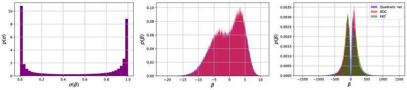
where the number of hidden neurons correspond to the minimal number required to match the rank of the BOC matrix , hence . Since this network is expressive enough to fully reproduce the BOC, our analysis in Section 3.1 holds, and the importance of eigenvalues and eigenvectors is manifest. We show the result of a quadratic network converging to the BOC in Figure 2 where .
5.2 Karush–Kuhn–Tucker (KKT) Convergence
Another source of intuition for the value of may be found in the KKT convergence equation (Ji and Telgarsky, 2020; Lyu and Li, 2020), which states, in a nutshell, that the weights of a homogeneous neural network 222Homogeneity, i.e. , where is the output of the network, are the network parameters, and , a quadratic network satisfies this requirement as it is composed of monomials., trained with the logistic loss for binary classification, using an infinitesimal learning rate and infinite iterations , will converge in direction to a KKT fixed point given by
| (14) |
where are the network weights at convergence, are the samples and are the sample labels. Here, , and are nonzero only for samples on the decision boundary. The full theorem and requirements are provided in Appendix B. We can apply Equation 14 to the quadratic network as
| (15) |
where we assume no biases (consistent with the case of similar spectrum and different basis). We posit, that in high dimensions , since at large every sample in the dataset should lie on the margin and contribute an equal amount, and the decision hyper-surface area should be comparable to the entire volume (Hsu et al., 2022). Under this ansatz, the above equations can be solved numerically, and indeed approximate the BOC as increases. We present evidence that the Bayes optimal decision boundary can be realized by a two-layer neural network with quadratic activation, and increasing the number of hidden units increases the probability of converging to this minima under gradient flow in Figure 2.
6 Results Extending to Realistic Data and Networks
In the previous section, we showed that small differences in eigenvalues and eigenvectors are magnified by the dimension, making classification easier. We further demonstrated that differences in the eigenvectors are faster growing in the dimension of the data, suggesting eigenvectors play a more significant role in the Bayesian decision boundary. Next, we will provide clear evidence that these conclusions hold, and extend to real-world datasets, by performing a set of tests related to the various properties of the covariance matrices. We train two common network architectures to perform binary classification, both on GMMs and on real images, exploring their performance as we change the covariance structure of each class.
Concretely, we consider two popular network architectures: fully connected (FC) and convolutional neural networks (CNN), tested on the CIFAR10 (Krizhevsky, 2012) and Fashion-MNIST (Xiao et al., 2017) datasets. For each training procedure, the model is optimized to classify samples from two classes in the given dataset (class 0 versus classes 1-9 aggregated).
The optimization procedure proceeds as follows: for each class, the samples are split into training and evaluation subsets. We then compute the covariance matrix of the training and evaluation subsets separately for the first and second classes. New synthetic data is generated by sampling from a multivariate Gaussian distribution with zero mean and the corresponding covariance matrix. This synthetic data is used to train the model to distinguish between the two classes (i.e. classify the Gaussians). When trained on real images, the model is tested on real images and not gaussians.
The optimization objective is the binary cross-entropy loss. The FC architecture consists of 3 dense layers with 2048 units each utilizing ReLU activations, followed by a softmax output layer. For CNNs, we employ ResNet-18 (He et al., 2015). All models are optimized with the Adam optimizer, a learning rate of 0.001, and Cosine Annealing LR scheduling over 50 epochs with a batch size of 256. The synthetic datasets contain 1,280 images per class, split 80-20 for training and validation. Our computational resource was a single NVIDIA GeForce GTX 1650 GPU, with 16GB RAM.
6.1 Tests on GMMs
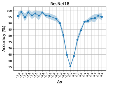
We first perform an experiment to quantitatively evaluate a network’s ability to utilize covariance matrix eigenvalue scaling for classification tasks. Specifically, two random covariance matrices are constructed using Equation 8, with one covariance has the spectral scaling of and the other of . Critically, both matrices share the same basis of eigenvectors. Approximately 500 samples are then drawn from each covariance matrix.
A model is trained to classify between the two classes defined by the distinct covariance matrices. Figure 3 shows the results for a fully connected network, as well as for a ResNet18 architecture (He et al., 2015). To assess the performance variability, the results are averaged over an ensemble of five independent training runs.
By varying only the scaling exponent between the covariances while keeping the eigenvectors fixed, this experiment protocol directly tests a network’s capability to leverage the eigenvalue scaling imparted by the covariance matrix for discriminative learning. The stability of the classifications indicate the degree to which these deep models can extract and utilize the intrinsic geometrical information encoded in the covariance descriptors.
6.2 Flip Tests on GMMs Constructed from Real Data
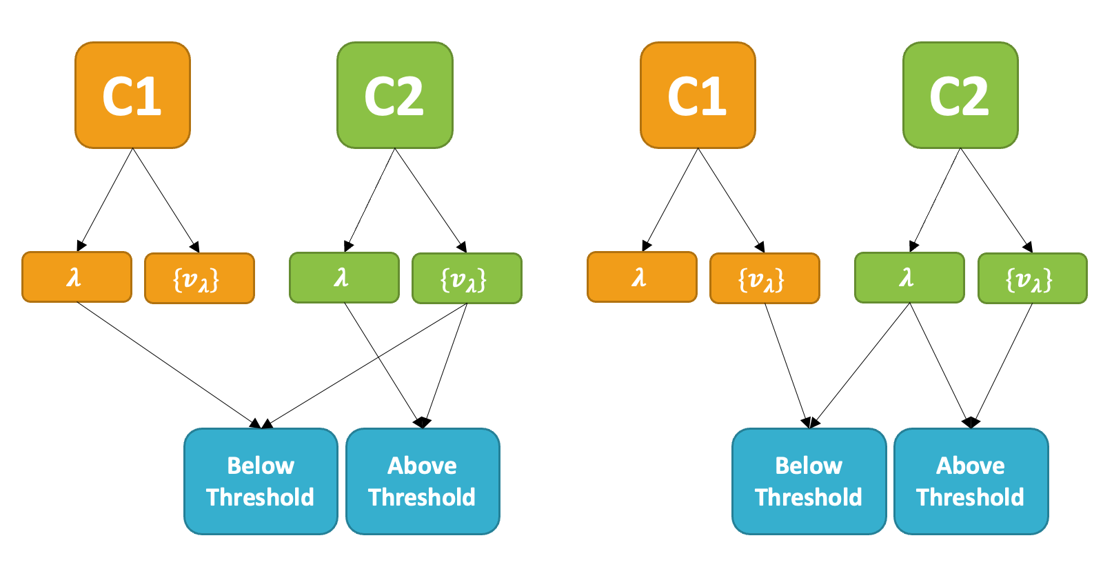
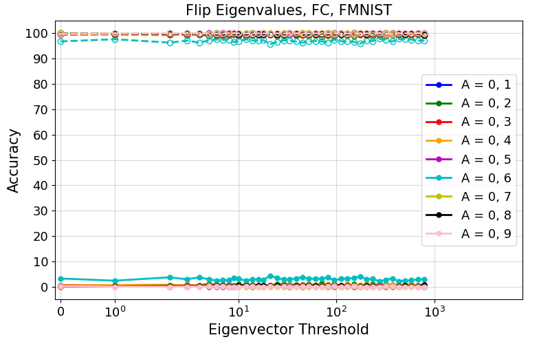
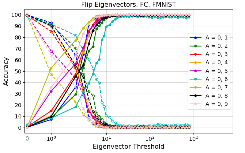
Next, we consider the role of eigenvectors and eigenvalues in classifying overlapping GMMs, as well as real images. It is known that the eigenvectors and eigenvalues of the data covariance matrix reveal different aspects of the data. In order to understand which of the two contains pertinent information for NN classification performance, we consider the following setup: we study two datasets, with covariance matrices and , and decompose each one of them to a set of eigenvectors and eigenvalues: , . We then construct a new covariance matrix by combining some of the eigenvalues and eigenvectors of and . To quantify the ratio of eigenvectors/eigenvalues coming from each class, we define two threshold indices for the eigenvalues and for the eigenvectors , where each of them is an integer between 0 and the dimension of , given by . The new covariance matrix reads:
| (16) |
where and are the new basis, and eigenvalues, respectively, which are composed by a mixture between the two classes:
| (17) |
This process is denoted as a flip test, illustrated in Figure 8.
It is worth noting that when composing the rotation matrix , we must ensure that it is nearly orthogonal to maintain the properties of a true basis, which is not guaranteed in our scheme. However, we find that this matrix is very close to orthogonal in the following sense: we define the following error, and require
| (18) |
where is the Frobenius norm. Equation 18 sets an upper bound for the error over all of the thresholds . We practically found that , while computing it for a randomly generated matrix composed of unit norm vectors gives .
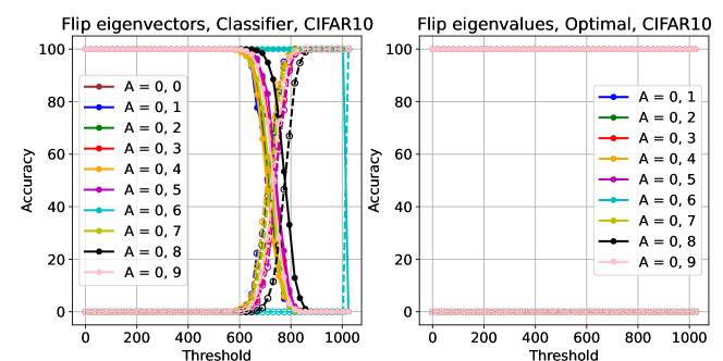
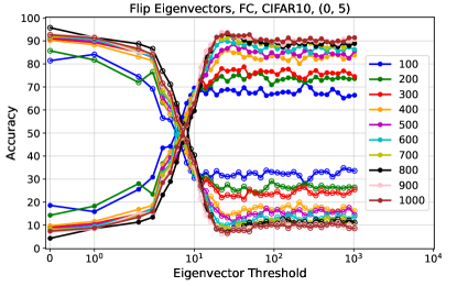
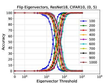
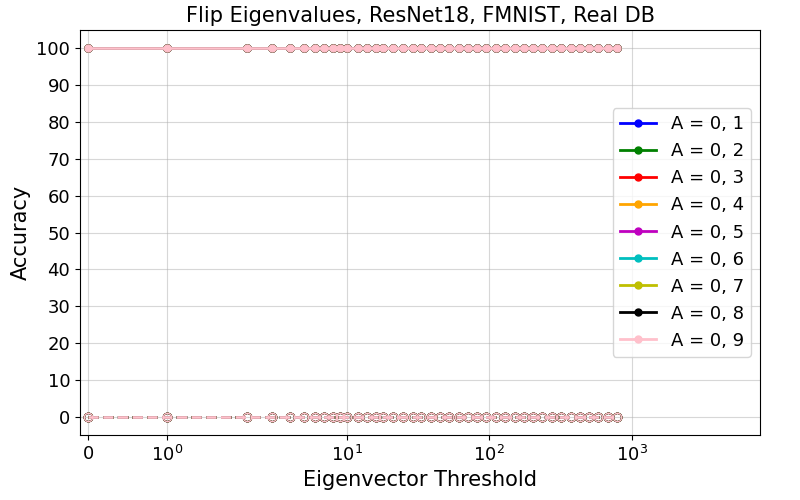
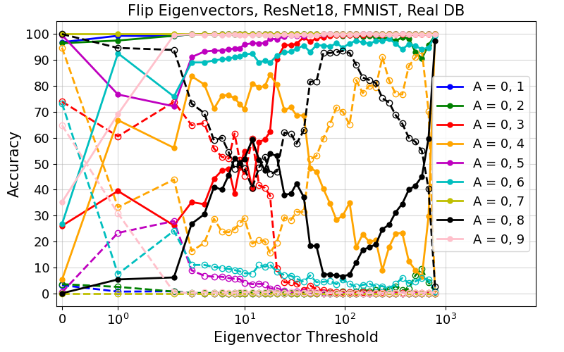
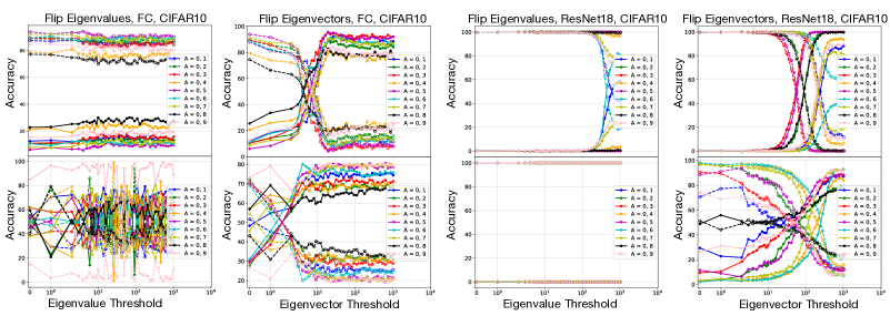
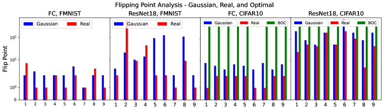
In Figure 4 (top row), we show the results of training a FC and ResNet18 networks to classify GMMs constructed from different and tested on samples drawn from . The baseline results are that the network classifies samples as coming from if has both the eigenvalues and eigenvectors of . When constructing with the eigenvectors of and the eigenvalues of , the network still classifies samples as coming from . This is not the case when taking the eigenvalues from but some of the eigenvectors from . Evidently, it requires a eigenvectors from to convince the network that the samples came from .
In Figure 4 (bottom row), we show that this result is architecture dependent, but the existence of an eigenvector flipping point persists throughout our experiments. We further compare this result with the BOC prediction, showing that indeed the BOC requires more eigenvectors to be flipped before determining that samples belong in rather than . This is shown in detail in Figure 11.
We further analyze the above flip tests for different data sizes used to construct and . We find that the results do not change above a certain number of samples, as the covariance matrices are well approximated beyond that point. Figure 12 shows the results.
6.3 Flip Tests on Real Data
To ensure that the overlapping mixture model holds for real-data, we examined the effect of adding the vector class means computed from the CIFAR10 and FMNIST datasets. We observed no qualitative change in the results, indicating that the assumption of zero mean is justified in these cases.
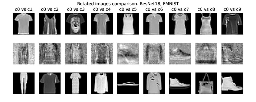
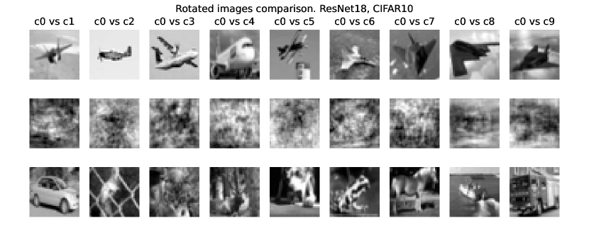
In order to perform the same flipping tests on real images, we simply perform a whitening transformation, followed by a rescaling, and then rotating to the basis of choice (Belhumeur et al., 1997). For an illustration of the resulting images see Figure 9 and Figure 10. This process ensures that the class covariance matrices of the data have been matched to our design, but inherently affects all the higher moments of the underlying distribution in an unpredictable way. Interestingly, as can be seen in Figure 4 (top row), the occurrence of a clear flipping point which depends on eigenvectors and not eigenvalues is manifest in real images. In Figure 4 (bottom row) we show a comparison between the thresholds for GMMs and real images, where the results indicate a close similarity, particularly for ResNet18 trained on CIFAR10, which can be attributed to its high expressivity.
7 Conclusions and Limitations
We studied binary classification of high dimensional overlapping GMM data as a framework to model real-world image datasets and to quantify the importance for the classification tasks of the eigenvalues and the eigenvectors of the data covariance matrix. We showed that deep neural networks trained for classification, learn predictors that approximate the Bayes optimal classifiers, and demonstrated that the decision thresholds for networks trained on authentic data correlate with the covariance eigenvectors rather than the eigenvalues, compatible with the GMM analysis. Our results reveal new theoretical insights to the neural networks’ ability to perform probabilistic inference and distill statistical patterns from complex distributions.
Limitations: Firstly, we focused on the regime of the estimated class covariances, while in many real-world cases, the empirical limit may be more applicable Levi and Oz (2023b). In Section 5.2, our ansatz neglected the dependence of on and the spectral density, which nonlinearly determines the number of points which lie on the decision surface. It might be possible to derive a similar result to Hsu et al. (2022) by taking a feature map approach to the quadratic net, but we postpone this to future work. Finally, while we quantified the significance of the detailed structure of the data covariance matrix, i.e. its eigenvalues and eigenvectors and their relative importance for classification, we are still left with the open question regarding the relative importance of the higher moments of the distribution, which we leave for a future study.
8 Acknowledgements
We would like to thank Amir Globerson, Yohai Bar-Sinai, Yue Lu and Bruno Loureiro for useful discussions. NL would like to thank G-Research for the award of a research grant, as well as the CERN-TH department for their hospitality during various stages of this work. The work of Y.O. is supported in part by Israel Science Foundation Center of Excellence.
References
- Donoho and Tanner (2009) David Donoho and Jared Tanner. Observed universality of phase transitions in high-dimensional geometry, with implications for modern data analysis and signal processing. Philosophical Transactions of the Royal Society A: Mathematical, Physical and Engineering Sciences, 367(1906):4273–4293, 2009.
- Korada and Montanari (2011) Satish Babu Korada and Andrea Montanari. Applications of the lindeberg principle in communications and statistical learning. IEEE Transactions on Information Theory, 57(4):2440–2450, 2011. doi: 10.1109/TIT.2011.2112231.
- Monajemi et al. (2013) Hatef Monajemi, Sina Jafarpour, Matan Gavish, David L. Donoho, Sivaram Ambikasaran, Sergio Bacallado, Dinesh Bharadia, Yuxin Chen, Young Choi, Mainak Chowdhury, Soham Chowdhury, Anil Damle, Will Fithian, Georges Goetz, Logan Grosenick, Sam Gross, Gage Hills, Michael Hornstein, Milinda Lakkam, Jason Lee, Jian Li, Linxi Liu, Carlos Sing-Long, Mike Marx, Akshay Mittal, Albert No, Reza Omrani, Leonid Pekelis, Junjie Qin, Kevin Raines, Ernest Ryu, Andrew Saxe, Dai Shi, Keith Siilats, David Strauss, Gary Tang, Chaojun Wang, Zoey Zhou, and Zhen Zhu. Deterministic matrices matching the compressed sensing phase transitions of gaussian random matrices. Proceedings of the National Academy of Sciences, 110(4):1181–1186, 2013. doi: 10.1073/pnas.1219540110.
- Candès et al. (2020) Emmanuel J Candès, Pragya Sur, et al. The phase transition for the existence of the maximum likelihood estimate in high-dimensional logistic regression. The Annals of Statistics, 48(1):27–42, 2020.
- Bartlett et al. (2020) Peter L. Bartlett, Philip M. Long, Gábor Lugosi, and Alexander Tsigler. Benign overfitting in linear regression. Proceedings of the National Academy of Sciences, 117(48):30063–30070, 2020. ISSN 0027-8424. doi: 10.1073/pnas.1907378117.
- Maloney et al. (2022) Alexander Maloney, Daniel A. Roberts, and James Sully. A solvable model of neural scaling laws, 2022.
- Kaplan et al. (2020) Jared Kaplan, Sam McCandlish, Tom Henighan, Tom B. Brown, Benjamin Chess, Rewon Child, Scott Gray, Alec Radford, Jeffrey Wu, and Dario Amodei. Scaling laws for neural language models, 2020.
- Seddik et al. (2020) Mohamed El Amine Seddik, Cosme Louart, Mohamed Tamaazousti, and Romain Couillet. Random matrix theory proves that deep learning representations of gan-data behave as gaussian mixtures, 2020.
- Montanari and Saeed (2022) Andrea Montanari and Basil N. Saeed. Universality of empirical risk minimization. In Proceedings of Thirty Fifth Conference on Learning Theory, volume 178 of Proceedings of Machine Learning Research, pages 4310–4312. PMLR, 02–05 Jul 2022.
- Mai and Liao (2019) Xiaoyi Mai and Zhenyu Liao. High-dimensional classification via empirical risk minimization: Improvements and optimality. arXiv: 1905.13742, 2019.
- Mignacco et al. (2020a) Francesca Mignacco, Florent Krzakala, Yue Lu, Pierfrancesco Urbani, and Lenka Zdeborova. The role of regularization in classification of high-dimensional noisy gaussian mixture. In International Conference on Machine Learning, pages 6874–6883. PMLR, 2020a.
- Taheri et al. (2020) Hossein Taheri, Ramtin Pedarsani, and Christos Thrampoulidis. Optimality of least-squares for classification in gaussian-mixture models. In 2020 IEEE International Symposium on Information Theory (ISIT), pages 2515–2520. IEEE, 2020.
- Kini and Thrampoulidis (2021) Ganesh Ramachandra Kini and Christos Thrampoulidis. Phase transitions for one-vs-one and one-vs-all linear separability in multiclass gaussian mixtures. In ICASSP 2021-2021 IEEE International Conference on Acoustics, Speech and Signal Processing (ICASSP), pages 4020–4024. IEEE, 2021.
- Wang and Thrampoulidis (2021) Ke Wang and Christos Thrampoulidis. Benign overfitting in binary classification of gaussian mixtures. In ICASSP 2021-2021 IEEE International Conference on Acoustics, Speech and Signal Processing (ICASSP), pages 4030–4034. IEEE, 2021.
- Refinetti et al. (2021) Maria Refinetti, Sebastian Goldt, Florent Krzakala, and Lenka Zdeborová. Classifying high-dimensional gaussian mixtures: Where kernel methods fail and neural networks succeed, 2021.
- Loureiro et al. (2021a) Bruno Loureiro, Gabriele Sicuro, Cedric Gerbelot, Alessandro Pacco, Florent Krzakala, and Lenka Zdeborova. Learning gaussian mixtures with generalized linear models: Precise asymptotics in high-dimensions. In Advances in Neural Information Processing Systems, volume 34, pages 10144–10157, 2021a.
- Mai et al. (2019) Xiaoyi Mai, Zhenyu Liao, and Romain Couillet. A Large Scale Analysis of Logistic Regression: Asymptotic Performance and New Insights. In ICASSP 2019 - 2019 IEEE International Conference on Acoustics, Speech and Signal Processing (ICASSP), pages 3357–3361, May 2019. doi: 10.1109/ICASSP.2019.8683376. ISSN: 2379-190X.
- Mignacco et al. (2020b) Francesca Mignacco, Florent Krzakala, Yue M. Lu, and Lenka Zdeborová. The role of regularization in classification of high-dimensional noisy gaussian mixture. 2020b. doi: 10.48550/ARXIV.2002.11544. URL https://arxiv.org/abs/2002.11544.
- Deng et al. (2022) Zeyu Deng, Abla Kammoun, and Christos Thrampoulidis. A model of double descent for high-dimensional binary linear classification. Information and Inference: A Journal of the IMA, 11(2):435–495, June 2022. ISSN 2049-8772. doi: 10.1093/imaiai/iaab002. URL https://doi.org/10.1093/imaiai/iaab002.
- Thrampoulidis et al. (2020) Christos Thrampoulidis, Samet Oymak, and Mahdi Soltanolkotabi. Theoretical insights into multiclass classification: a high-dimensional asymptotic view. In Proceedings of the 34th International Conference on Neural Information Processing Systems, NIPS’20, pages 8907–8920, Red Hook, NY, USA, December 2020. Curran Associates Inc. ISBN 9781713829546.
- Loureiro et al. (2021b) Bruno Loureiro, Gabriele Sicuro, Cédric Gerbelot, Alessandro Pacco, Florent Krzakala, and Lenka Zdeborová. Learning gaussian mixtures with generalised linear models: Precise asymptotics in high-dimensions. 2021b. doi: 10.48550/ARXIV.2106.03791. URL https://arxiv.org/abs/2106.03791.
- Couillet et al. (2018) Romain Couillet, Zhenyu Liao, and Xiaoyi Mai. Classification asymptotics in the random matrix regime. In 2018 26th European Signal Processing Conference (EUSIPCO), pages 1875–1879, 2018. doi: 10.23919/EUSIPCO.2018.8553034.
- Liao and Couillet (2019) Zhenyu Liao and Romain Couillet. A large dimensional analysis of least squares support vector machines. IEEE Transactions on Signal Processing, 67(4):1065–1074, February 2019. ISSN 1941-0476. doi: 10.1109/tsp.2018.2889954. URL http://dx.doi.org/10.1109/TSP.2018.2889954.
- Kammoun and Couillet (2023) Abla Kammoun and Romain Couillet. Covariance discriminative power of kernel clustering methods. Electronic Journal of Statistics, 17(1):291 – 390, 2023. doi: 10.1214/23-EJS2107. URL https://doi.org/10.1214/23-EJS2107.
- Loureiro et al. (2021c) Bruno Loureiro, Gabriele Sicuro, Cedric Gerbelot, Alessandro Pacco, Florent Krzakala, and Lenka Zdeborová. Learning gaussian mixtures with generalized linear models: Precise asymptotics in high-dimensions. In M. Ranzato, A. Beygelzimer, Y. Dauphin, P.S. Liang, and J. Wortman Vaughan, editors, Advances in Neural Information Processing Systems, volume 34, pages 10144–10157. Curran Associates, Inc., 2021c. URL https://proceedings.neurips.cc/paper_files/paper/2021/file/543e83748234f7cbab21aa0ade66565f-Paper.pdf.
- Ingrosso and Goldt (2022) Alessandro Ingrosso and Sebastian Goldt. Data-driven emergence of convolutional structure in neural networks. Proceedings of the National Academy of Sciences, 119(40), September 2022. ISSN 1091-6490. doi: 10.1073/pnas.2201854119. URL http://dx.doi.org/10.1073/pnas.2201854119.
- Elkhalil et al. (2017) Khalil Elkhalil, Abla Kammoun, Romain Couillet, Tareq Y Al-Naffouri, and Mohamed-Slim Alouini. Asymptotic performance of regularized quadratic discriminant analysis based classifiers. In 2017 IEEE 27th International Workshop on Machine Learning for Signal Processing (MLSP), pages 1–6. IEEE, 2017.
- Ghojogh and Crowley (2019) Benyamin Ghojogh and Mark Crowley. Linear and quadratic discriminant analysis: Tutorial, 2019.
- Das and Geisler (2021) Abhranil Das and Wilson S. Geisler. A method to integrate and classify normal distributions. Journal of Vision, 21(10):1, September 2021. ISSN 1534-7362. doi: 10.1167/jov.21.10.1. URL http://dx.doi.org/10.1167/jov.21.10.1.
- Schilling et al. (2021) Achim Schilling, Andreas Maier, Richard Gerum, Claus Metzner, and Patrick Krauss. Quantifying the separability of data classes in neural networks. Neural Networks, 139:278–293, July 2021. ISSN 0893-6080. doi: 10.1016/j.neunet.2021.03.035. URL http://dx.doi.org/10.1016/j.neunet.2021.03.035.
- Ferrari (2019) Alberto Ferrari. A note on sum and difference of correlated chi-squared variables, 2019.
- Biroli and Mézard (2023) Giulio Biroli and Marc Mézard. Generative diffusion in very large dimensions. Journal of Statistical Mechanics: Theory and Experiment, 2023(9):093402, September 2023. ISSN 1742-5468. doi: 10.1088/1742-5468/acf8ba. URL http://dx.doi.org/10.1088/1742-5468/acf8ba.
- Tiomoko et al. (2019) Malik Tiomoko, Romain Couillet, Eric Moisan, and Steeve Zozor. Improved estimation of the distance between covariance matrices. In ICASSP 2019 - 2019 IEEE International Conference on Acoustics, Speech and Signal Processing (ICASSP), pages 7445–7449, 2019. doi: 10.1109/ICASSP.2019.8682621.
- Zhang et al. (2018) Guodong Zhang, Chaoqi Wang, Bowen Xu, and Roger B. Grosse. Three mechanisms of weight decay regularization. CoRR, abs/1810.12281, 2018. URL http://arxiv.org/abs/1810.12281.
- Levi and Oz (2023a) Noam Levi and Yaron Oz. The underlying scaling laws and universal statistical structure of complex datasets. arXiv preprint arXiv:2306.14975, 2023a.
- Loureiro et al. (2021d) Bruno Loureiro, Cedric Gerbelot, Hugo Cui, Sebastian Goldt, Florent Krzakala, Marc Mezard, and Lenka Zdeborova. Learning curves of generic features maps for realistic datasets with a teacher-student model. In Advances in Neural Information Processing Systems, volume 34, 2021d.
- Loureiro et al. (2022) Bruno Loureiro, Cedric Gerbelot, Hugo Cui, Sebastian Goldt, Florent Krzakala, Marc Mezard, and Lenka Zdeborova. Learning curves of generic features maps for realistic datasets with a teacher-student model. Journal of Statistical Mechanics: Theory and Experiment, 2022(11):114001, nov 2022. doi: 10.1088/1742-5468/ac9825. URL https://doi.org/10.1088%2F1742-5468%2Fac9825.
- Radhakrishnan et al. (2023) Adityanarayanan Radhakrishnan, Mikhail Belkin, and Caroline Uhler. Wide and deep neural networks achieve consistency for classification. Proceedings of the National Academy of Sciences, 120(14), March 2023. ISSN 1091-6490. doi: 10.1073/pnas.2208779120. URL http://dx.doi.org/10.1073/pnas.2208779120.
- Jaganathan et al. (2015) Kishore Jaganathan, Yonina C. Eldar, and Babak Hassibi. Phase retrieval: An overview of recent developments, 2015.
- Dong et al. (2023) Jonathan Dong, Lorenzo Valzania, Antoine Maillard, Thanh-an Pham, Sylvain Gigan, and Michael Unser. Phase retrieval: From computational imaging to machine learning: A tutorial. IEEE Signal Processing Magazine, 40(1):45–57, 2023. doi: 10.1109/MSP.2022.3219240.
- Candes et al. (2014) Emmanuel J. Candes, Xiaodong Li, and Mahdi Soltanolkotabi. Phase retrieval via wirtinger flow: Theory and algorithms. CoRR, abs/1407.1065, 2014. URL http://arxiv.org/abs/1407.1065.
- Chen et al. (2019) Yuxin Chen, Yuejie Chi, Jianqing Fan, and Cong Ma. Gradient descent with random initialization: fast global convergence for nonconvex phase retrieval. Mathematical Programming, 176(1–2):5–37, February 2019. ISSN 1436-4646. doi: 10.1007/s10107-019-01363-6. URL http://dx.doi.org/10.1007/s10107-019-01363-6.
- Arnaboldi et al. (2024) Luca Arnaboldi, Florent Krzakala, Bruno Loureiro, and Ludovic Stephan. Escaping mediocrity: how two-layer networks learn hard generalized linear models with sgd, 2024.
- Martin et al. (2023) Simon Martin, Francis Bach, and Giulio Biroli. On the impact of overparameterization on the training of a shallow neural network in high dimensions, 2023.
- Livni et al. (2014) Roi Livni, Shai Shalev-Shwartz, and Ohad Shamir. On the computational efficiency of training neural networks, 2014.
- Soltani and Hegde (2018) Mohammadreza Soltani and Chinmay Hegde. Towards provable learning of polynomial neural networks using low-rank matrix estimation. In Amos Storkey and Fernando Perez-Cruz, editors, Proceedings of the Twenty-First International Conference on Artificial Intelligence and Statistics, volume 84 of Proceedings of Machine Learning Research, pages 1417–1426. PMLR, 09–11 Apr 2018. URL https://proceedings.mlr.press/v84/soltani18a.html.
- Ji and Telgarsky (2020) Ziwei Ji and Matus Telgarsky. Directional convergence and alignment in deep learning, 2020.
- Lyu and Li (2020) Kaifeng Lyu and Jian Li. Gradient descent maximizes the margin of homogeneous neural networks, 2020.
- Hsu et al. (2022) Daniel Hsu, Vidya Muthukumar, and Ji Xu. On the proliferation of support vectors in high dimensions, 2022.
- Krizhevsky (2012) Alex Krizhevsky. Learning multiple layers of features from tiny images. University of Toronto, 05 2012. URL https://www.cs.toronto.edu/~kriz/learning-features-2009-TR.pdf.
- Xiao et al. (2017) Han Xiao, Kashif Rasul, and Roland Vollgraf. Fashion-mnist: A novel image dataset for benchmarking machine learning algorithms. arXiv: 1708.07747, 2017. doi: 10.48550/ARXIV.1708.07747.
- He et al. (2015) Kaiming He, Xiangyu Zhang, Shaoqing Ren, and Jian Sun. Deep residual learning for image recognition, 2015.
- Belhumeur et al. (1997) Peter N. Belhumeur, João P. Hespanha, and David J. Kriegman. Eigenfaces vs. fisherfaces: Recognition using class specific linear projection. IEEE Trans. Pattern Anal. Mach. Intell., 19(7):711–720, jul 1997. ISSN 0162-8828. doi: 10.1109/34.598228. URL https://doi.org/10.1109/34.598228.
- Levi and Oz (2023b) Noam Levi and Yaron Oz. The universal statistical structure and scaling laws of chaos and turbulence. arXiv preprint arXiv:2311.01358, 2023b.
- Papyan et al. (2020) Vardan Papyan, X. Y. Han, and David L. Donoho. Prevalence of neural collapse during the terminal phase of deep learning training. Proceedings of the National Academy of Sciences, 117(40):24652–24663, September 2020. ISSN 1091-6490. doi: 10.1073/pnas.2015509117. URL http://dx.doi.org/10.1073/pnas.2015509117.
Appendix A Neural Collapse on Overlapping GMM Data
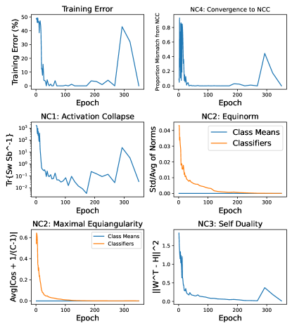
Here, we explore the concept of Neural Collapse (NC) on overlapping GMMs generated from real data. Practically, we employ the metrics given in Papyan et al. [2020] to measure the NC when training a ResNet18 on gaussian versions of CIFAR10 images. In Figure 5, we show that NC occurs on overlapping GMMs even when the class mean vector of the data has been set to zero, indicating that expressive networks are able to perform nonlinear transformations that generate class means, where none were present, and at the final layer still perform linear classification.
Various metrics of Neural Collapse, as given by Papyan et al. [2020], are shown for GMMs generated from two classes of CIFAR10. Here, we use 5000 samples per class, training a ResNet18 to perform binary classification using cross-entropy loss, on GMMs generated from greyscale versions of CIFAR10 images. Each sample has dimension , and the training is done using the default specifications provided in the supplementary code of Papyan et al. [2020]
Appendix B KKT formulation
As discussed in the main text, we posit that the approach towards a BOC for a NN can be explained by convergence to a KKT point.
Our reasoning follows Theorem Theorem B.1 below, which holds for gradient flow (i.e., gradient descent with an infinitesimally small step size). Before stating the theorem, we need the following definitions: (1) We say that gradient flow converges in direction to if , where is the parameter vector at time ; (2) We say that a network is homogeneous w.r.t. the parameters if there exists such that for every and we have . Thus, scaling the parameters by any factor scales the outputs by . We note that essentially any fully-connected or convolutional neural network with ReLU activations is homogeneous w.r.t. the parameters if it does not have any skip-connections (i.e., residual connections) or bias terms, except possibly for the first layer.
Theorem B.1 (Paraphrased from Lyu and Li [2020], Ji and Telgarsky [2020]).
Let be a homogeneous ReLU neural network. Consider minimizing the logistic loss over a binary classification dataset using gradient flow. Assume that there exists time such that 333This ensures that for all , i.e. at some time classifies every sample correctly.. Then, gradient flow converges in direction to a first order stationary point (KKT point) of the following maximum-margin problem:
| (19) |
Moreover, as .
The above theorem guarantees directional convergence to a first order stationary point (of the optimization problem (Equation 19)), which is also called Karush–Kuhn–Tucker point, or KKT point for short. The KKT approach allows inequality constraints, and is a generalization of the method of Lagrange multipliers, which allows only equality constraints.
The great virtue of Theorem B.1 is that it characterizes the implicit bias of gradient flow with the logistic loss for homogeneous networks. Namely, even though there are many possible directions of that classify the dataset correctly, gradient flow converges only to directions that are KKT points of Problem (Equation 19). In particular, if the trajectory of gradient flow under the regime of Theorem B.1 converges in direction to a KKT point , then we have the following: There exist such that
| (stationarity) | (20) | |||
| (primal feasibility) | (21) | |||
| (dual feasibility) | (22) | |||
| (complementary slackness) | (23) |
Our main insight is based on Equation 20, which implies that the parameters are a linear combinations of the derivatives of the network at the training data points. We say that a data point is on the margin if (i.e. ) . Note that Equation 23 implies that only samples which are on the margin affect Equation 20, since samples not on the margin have a coefficient . In sufficiently high dimension we expect no samples to be off the margin in GMM classification therefore all should be nonzero and contribute a similar amount.
Appendix C Dataset Properties
We show the eigenvalues scaling structure and the Inverse Participation Ratio (IPR) of the eigenvectors. We separate the eigenvalues to three parts: I. The large eigenvalues, II. The bulk eigenvalues, and III. The small eigenvalues, as can be seen in Figure 6. These three regimes are seen also in real datasets as shown in previous work [Levi and Oz, 2023a, b]. Figure 6 shows the eigenvalues for each of the classes in the FMNIST and CIFAR10 datasets, respectively.
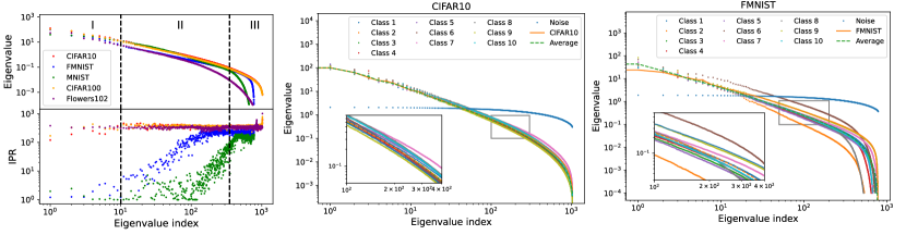
The IPR defined as:
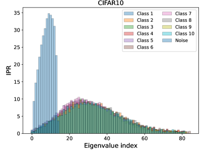
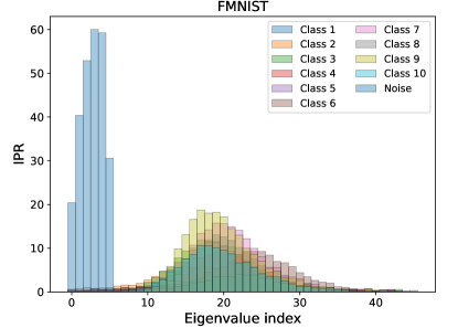
| (24) |
is used to measure the localization rate (entropy) of a vector. Figure 7 shows the IPR of the eigenvectors of the covariance matrices for the different classes in the CIFAR10 dataset and FMNIST. As can be seen from the Figure, the changes in the eigenvalues structure and the IPR is small.
Appendix D Appendix - Flipping tests examples
We include the different figures concerning the classification flipping tests referred to in the main text. The diagram in Figure 8 outlines the structure of the flipping tests. In Figure 9 and Figure 10 we see rotated images of FMNIST and CIFAR10, respectively. In Figure 11, Figure 12 and Figures 13 and 14 we plot the eigenvalues and eigenvectors thresholds.
The code for our experiments is provded in https://github.com/khencohen/FlippingsTests.