GFlow: Recovering 4D World from Monocular Video

Abstract

Reconstructing 4D scenes from video inputs is a crucial yet challenging task. Conventional methods usually rely on the assumptions of multi-view video inputs, known camera parameters, or static scenes, all of which are typically absent under in-the-wild scenarios. In this paper, we relax all these constraints and tackle a highly ambitious but practical task, which we termed as AnyV4D: we assume only one monocular video is available without any camera parameters as input, and we aim to recover the dynamic 4D world alongside the camera poses. To this end, we introduce GFlow, a new framework that utilizes only 2D priors (depth and optical flow) to lift a video (3D) to a 4D explicit representation, entailing a flow of Gaussian splatting through space and time. GFlow first clusters the scene into still and moving parts, then applies a sequential optimization process that optimizes camera poses and the dynamics of 3D Gaussian points based on 2D priors and scene clustering, ensuring fidelity among neighboring points and smooth movement across frames. Since dynamic scenes always introduce new content, we also propose a new pixel-wise densification strategy for Gaussian points to integrate new visual content. Moreover, GFlow transcends the boundaries of mere 4D reconstruction; it also enables tracking of any points across frames without the need for prior training and segments moving objects from the scene in an unsupervised way. Additionally, the camera poses of each frame can be derived from GFlow, allowing for rendering novel views of a video scene through changing camera pose. By employing the explicit representation, we may readily conduct scene-level or object-level editing as desired, underscoring its versatility and power. Visit our project website at: littlepure2333.github.io/GFlow.

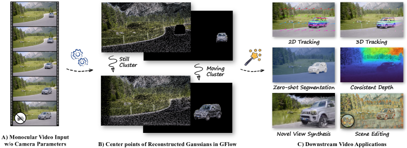
Figure 1: A) Given a monocular video in the wild, B) our proposed GFlow can reconstruct the underlying 4D world, i.e. the dynamic scene represented by 3D Gaussian splatting [10] and associated camera poses. The Gaussians are split into still and moving clusters and are densified within GFlow. C) From GFlow we can straightforwardly enable various capacities, such as tracking, segmentation, novel view synthesis, and editing. Best viewed by zooming in.

1 Introduction

The quest for accurate reconstruction of 4D worlds (3D + t) from video inputs stands at the forefront of contemporary research in computer vision and graphics. This endeavor is crucial for the advancement of virtual and augmented reality, video analysis, and multimedia applications. The challenge primarily stems from capturing the transient essence of dynamic scenes and the often absent camera pose information. Traditional approaches are typically split between two types: one relies on pre-calibrated camera parameters or multi-view video inputs to reconstruct dynamic scenes [35, 17, 30, 1, 3, 5, 12, 15, 16, 25], while the other estimates camera poses from static scenes using multi-view stereo techniques [2, 6, 32, 14, 34, 36, 27, 26, 31, 4]. This division highlights a missing piece in this field:

Is it possible to reconstruct dynamic 3D scenes and camera motion from a single, uncalibrated video input along?

We name this task "Any Video-to-4D", or "AnyV4D" for short. Addressing this challenge is particularly difficult due to the problem’s inherent complexity. Attempting to reconstruct dynamic 3D worlds from single-camera footage involves deciphering a puzzle where multiple solutions might visually seem correct but do not adhere to the physical composition of our world. Although NeRF-based methods attempt to solve this problem, they fall short of accurately capturing the physical constraints of the real world. This limitation stems from their implicit representation, which struggles to encode the underlying physical properties of materials and enforce real-world physical interactions.

Recent developments in 3D Gaussian Splatting (3DGS) [10] and its extensions [35, 17, 40, 39] into dynamic scenes have emerged as promising alternatives. These techniques have shown promise in handling the complexities associated with the dynamic nature of real-world scenes and the intricacies of camera movement and positioning. Yet, they still operate under the assumption of a known camera sequence [27, 26]. To overcome these limitations and unlock the full potential of dynamic scene reconstruction, we propose a new approach based on the following insight:

Given 2D characters such as RGB, depth and optical flow from one video, we actually have enough clues to model the 4D (3D+t) world behind the video(2D+t).

Based on this intuition, we introduce "GFlow", a novel framework that leverages the explicit representation power of 3D Gaussian Splatting [10] and conceptualizes the video content as a fluid flow of Gaussian points through space and time, effectively reconstructing a 4D world without direct camera input.

The key to GFlow is conducting scene clustering that separates the scene into still and moving parts, followed by a sequential optimization process that seamlessly integrates precise tuning of camera poses with dynamic adjustments of 3D Gaussian points. This dual optimization utilizes depth and optical flow priors to ensure that each video frame is accurately rendered, mirroring the dynamic flux of the original scene while incorporating new visual information through our newly designed pixel-wise densification strategy. This framework not only maintains cross-frame rendering fidelity but also ensures smooth transitions and movements among points, addressing the critical challenge of temporal coherence.

Moreover, through our experiments, GFlow has demonstrated not just its potential as a tool for 3D scene recovery but as a transformative force in video analysis and manipulation. Its ability to track any points across frames in 3D world coordinates without prior training and segment moving objects from the scene in an unsupervised manner redefines the landscape of video understanding. By employing explicit representation through 3DGS, GFlow can render enthralling new views of video scenes by easily changing camera poses and editing objects or entire scenes as desired, showcasing its unparalleled versatility and power.

2 Preliminaries

2.1 3D gaussian splatting

3D Gaussian Splatting (3DGS) [10] exhibits strong performance and efficiency in recent advances in 3D representation. 3DGS fits a scene as a set of Gaussians $\{G_{i}\}$ from multi-view images $\{V_{k}\}$ and paired camera poses $\{P_{k}\}$ in an optimization pipeline. Adaptive densification and pruning of Gaussians are applied in this iterative optimization to control the total number of Gaussians. Generally, each Gaussian is composed of its center coordinate $\mu\in\mathbb{R}^{3}$, 3D scale $s\in\mathbb{R}^{3}$, opacity $\alpha\in\mathbb{R}$, rotation quaternion $q\in\mathbb{R}^{4}$, and associated view-dependent color represented as spherical harmonics $c\in\mathbb{R}^{3(d+1)^{2}}$, where $d$ is the degree of spherical harmonics.

These parameters can be collectively denoted by $G$, with $G_{i}=\{\mu_{i},s_{i},\alpha_{i},q_{i},c_{i}\}$ denoting the parameters of the $i$-th Gaussian. The core of 3DGS is its tile-based differentiable rasterization pipeline to achieve real-time optimization and rendering. To render $\{G_{i}\}$ into a 2D image, each Gaussian is first projected into the camera coordinate frame given the camera pose $P_{i}$ to determine the depth of each Gaussian. Then colors, depth, or other attributes in pixel space are rendered in parallel by alpha composition with the depth order of adjacent 3D Gaussians. Specifically, in our formulation, we do not consider view-dependent color variations for simplicity, thus the degree of spherical harmonics is set as $d=0$, i.e., only the RGB color $c\in\mathbb{R}^{3}$.

2.2 Camera model

To project the 3D point coordinates $\mu\in\mathbb{R}^{3}$ into the camera view, we use the pinhole camera model. The camera intrinsics is $K\in\mathbb{R}^{3\times 3}$ and the camera extrinsics which define the world-to-camera transformation is $E=[R|t]\in\mathbb{R}^{3\times 4}$. The camera-view 2D coordinates $x\in\mathbb{R}^{2}$ are calculated as $dh(x)=KEh(\mu)$, where $d\in\mathbb{R}$ is the depth, and $h(\cdot)$ represents the homogeneous coordinate mapping.

3 Recovering 4D World as Gaussian Flow

Problem definition

The task "Any Video-to-4D", short for "AnyV4D" is defined as: Given a set of image frames taken from a monocular video input without any camera parameters, the goal is to create a model that represents the video’s 4D world. This model includes the 3D scene dynamics and the camera pose for each frame. The main challenge of this task is the complexity of video dynamics, which require simultaneously recovery of both camera pose and scene content.

Figure 2: Overview of GFlow. A) Given a monocular video input consisting of image sequence $\{I_{i}\}$, the associated depth $\{D_{i}\}$, optical flow $\{F_{i}\}$ and camera intrinsic $K$ are obtained using off-the-shelf prior. B) For each frame , GFLow first clustering the scene into still part $G_{i}^{s}$ and moving part $G_{i}^{m}$. Then optimization process in GFlow consists of two steps: C1) Only the camera pose $P_{t}$ is optimized by aligning the depth and optical flow within the still cluster. C2) Under the optimized camera pose $P_{t}^{*}$, the Gaussian points $\{G_{i}\}$ are optimized and densified based on RGB, depth, optical flow and the two scene clusters. D) The same procedure of steps B, C1, and C2 loops for the next frame. The colorful graphics under the dashed line represent the variables involved in the optimization.

Overview

To deal with above challenges, we propose GFlow, a framework that represent the videos through a flow of 3D Gaussian splatting [10]. At it essence, GFlow alternately optimizes the camera pose and Gaussian points for each frame in sequential order to reconstruct the 4D world. This process involves clustering Gaussian points into moving and still categories, along with densification of Gaussian points. The camera poses are determined based on the still points, while the moving points are optimized to accurately represent dynamic content in the video.

Pipeline

As shown in Figure 2, given an image sequence $\{I_{t}\}_{t=0}^{T}$ of monocular video input, we first utilizes off-the-shelf algorithms [38, 37, 32] to derive the corresponding depth $\{D_{t}\}_{t=0}^{T}$, optical flow $\{F_{t}\}_{t=0}^{T}$ and camera intrinsic $K$. The initialization of the Gaussians is performed using the prior-driven initialization, as described in Sec 3.2.1. Then for each frame $I_{t}$ at time $t$, GFlow first divides the Gaussian points $\{G_{i}\}_{t}$ into still cluster $\{G_{i}^{s}\}_{t}$ and moving cluster $\{G_{i}^{m}\}_{t}$ in Sec 3.1.1. The optimization process then proceeds in two steps. In the first step, only the camera extrinsics $E_{t}$ is optimized. This is achieved by aligning the Gaussian points within the still cluster with the depth $D_{t}$ and optical flow $F_{t-1}$, in Sec 3.1.2. Following this, under the optimized camera extrinsics $E_{t}^{*}$, the Gaussian points $G_{t}$ are further refined using constraints from the RGB $I_{t}$, depth $D_{t}$, optical flow $F_{t-1}$, in Sec 3.1.3. Additionally, the Gaussian points are densified using our proposed pixel-wise strategy to incorporate newly visible scene content, as outlined in Sec 3.2.2. After optimizing the current frame, the procedure — scene clustering, camera optimization, and Gaussian point optimization — is repeated for subsequent frames.

3.1 Alternating Gaussian-camera optimization

While the 3D Gaussian Splatting (3DGS) method [10] is adept at modeling static scenes, we have expanded its capabilities to represent videos by simulating a flow of Gaussian points through space and time. In this approach, the Gaussian points are initialized and optimized directly in the first frame as described in Sec 3.2.1. For subsequent frames, we adopt a alternating optimization strategy for the camera poses $\{P_{i}\}$ and the Gaussians $\{G_{i}\}$. This method allows us to effectively account for both camera movement and dynamic changes in the scene content.

3.1.1 Scene clustering

In constructing dynamic scenes that include both camera and object movements, treating these scenes as static can lead to inaccuracies and loss of crucial temporal information. To better manage this, we propose a method to cluster the scene into still and moving parts, which will be Incorporated in the optimisation stage.

At time $t$, We first employ K-Means [7] algorithm to separate Gaussian points into two groups based on their movements from the optical flow [38, 37] map map $F_{t}$. We assume the still part covers the most areas in the visual content. So the cluster with the larger area in the image, identified by its concave hull [20], is considered the still cluster $\{G_{i}^{s}\}_{t}\subseteq\{G_{i}\}_{t}$. The other is the moving cluster $\{G_{i}^{m}\}_{t}\subseteq\{G_{i}\}_{t}$.

In the first frame, we cluster the Gaussian points using this method. For later frames, as new points are added through densification, we need to update the clusters. Existing points keep their previous labels. For new points, we first cluster all points together. The new Gaussian point is labeled as ‘still’ if its current belonging cluster share the most common Guassian points with last frame’s still cluster $\{G_{i}^{s}\}_{t-1}$; otherwise, it’s labeled ‘moving’.

3.1.2 Camera optimization

Between two consecutive frames, we assume the camera intrinsic keep the same, while camera extrinsic undergo a slight transformation. Our goal is to identify and capture this transformation to maintain geometric consistency for elements in the scene that do not move.

We start with the assumption that the camera intrinsic, denoted as $K$, is known and derived from a widely-used stereo model [32]. The camera extrinsic $E=[R|t]$ consists of a rotation $R\in\mathbf{SO}(3)$ and a translation $t\in\mathbb{R}^{3}$.

For a given frame at time $t$, we optimize the camera extrinsic $E_{t}$ by minimizing the errors in its depth estimation and optical flow. During this optimization, only the Gaussian points within the still cluster $\{G_{i}^{s}\}_{t}$ are considered in the error calculation.

$$E_{t}^{*}=\mathop{\arg\min}\limits_{E_{t}}\Big{\{}\lambda_{d}\mathcal{L}_{dep}(\{G_{i}^{s}\}_{t},E_{t})+\lambda_{f}\mathcal{L}_{flo}(\{G_{i}^{s}\}_{t},E_{t})\Big{\}},$$ (1)

where $\lambda_{d}$ and $\lambda_{f}$ are weighting factors for depth loss $\mathcal{L}_{dep}$ and flow loss $\mathcal{L}_{flo}$, respectively.

Depth loss. The depth loss, $\mathcal{L}_{dep}$, is calculated using the L1 loss between the estimated and actual depths of Gaussian points. Specifically, for each Gaussian point $G_{i,t}$ within the cluster $\{G_{i}^{s}\}_{t}$ at time $t$, we define $d(G_{i,t};E_{t})$ as its depth from the camera and $x(G_{i,t};E_{t})$ as its projected 2D coordinate in the image. The corresponding depth from the depth map $D_{t}$ at these coordinates is $D_{t}(x(G_{i,t};E_{t}))$. To address discrepancies in scale between the estimated and actual depths, the loss is normalized by the sum of these two depth values.

The formal expression for the depth loss, considering all Gaussian points in the still cluster $\{G_{i}^{s}\}_{t}$ with respect to the extrinsic $E_{t}$ is given by:

$$\mathcal{L}_{dep}(\{G_{i}\}_{t},E_{t})=\sum_{\forall G_{i,t}\in\{G_{i}\}_{t}}\frac{|d(G_{i,t};E_{t})-D_{t}(x(G_{i,t};E_{t}))|}{d(G_{i,t};E_{t})+D_{t}(x(G_{i,t};E_{t}))};$$ (2)

Optical flow loss. The optical flow loss, denoted by $\mathcal{L}_{flo}$, quantifies the mean squared error (MSE) between the actual movements of Gaussian points between frames and the expected optical flow, ensuring the temporal smoothness of the Gaussian flow. Specifically, the loss compares the positional change of a Gaussian point, $x(G_{i,t};E_{t})-x(G_{i,t-1};E_{t})$, with the optical flow $F_{t-1}(x(G_{i,t-1};E_{t}))$ from the previous frame:

$$\mathcal{L}_{flo}(\{G_{i}\}_{t},E_{t})=\sum_{\forall G_{i,t}\in\{G_{i}\}_{t}}\Big{|}\Big{|}\big{(}x(G_{i,t};E_{t})-x(G_{i,t-1};E_{t})\big{)}-F_{t-1}\big{(}x(G_{i,t-1};E_{t})\big{)}\Big{|}\Big{|}_{2}^{2};$$ (3)

3.1.3 Gaussians optimization

In this section, we focus on optimizing Gaussian points in a scene at a specific time $t$, with optimized camera extrinsics $E_{t}^{*}$. Initially, we update the positions of the Gaussian points to reflect movement detected in previous frame. Subsequently, we optimize these points to ensure they align with the scene in terms of RGB appearance, depth, and optical flow.

Pre-optimization gaussian relocation.

Once we have the optimized camera extrinsics $E_{t}^{*}$, we proceed with updating the positions of moving Gaussian points. Initially, we track the 2D coordinates of moving Gaussian points from the previous frame $\{x(G_{i,t-1}^{m})\}$. Using these coordinates, we calculate their movement based on the previous frame’s optical flow map $\{F_{t-1}(x(G_{i,t-1}^{m}))\}$ and update their current position: $x(G_{i,t}^{m})=x(G_{i,t-1}^{m})+F_{t-1}(x(G_{i,t-1}^{m}))$. With the updated coordinates, we then extract the depth from the current frame’s depth map $\{D_{t}(x(G_{i,t}^{m}))\}$, and project these points from the camera view to world coordinates using $E_{t}^{*}$. This step ensures that the moving Gaussian points are accurately positioned for subsequent optimization.

Optimization objectives

The primary focus in optimizing Gaussian points is on minimizing photometric loss, which combines MSE and structural similarity index (SSIM) [33] between the rendered image from Gaussian points and the actual frame image $I_{t}$.

$$\mathcal{L}_{pho}(\{G_{i}\}_{t})=\mathcal{L}_{mse}(\mathcal{R}(\{G_{i}\}_{t}),I_{t})+\mathcal{L}_{ssim}(\mathcal{R}(\{G_{i}\}_{t}),I_{t});$$ (4)

Here, $\mathcal{R}(\cdot)$ denotes the 3D Gaussian splatting rendering process. To maintain the positional consistency of still Gaussian points, a stillness loss is implemented to minimize changes in their 3D center $\{\mu(G_{i},t)\}$ coordinates between frames:

$$\mathcal{L}_{sti}(\{G_{i}\}_{t})=\sum_{\forall G_{i,t}\in\{G_{i}\}_{t}}||\mu(G_{i,t})-\mu(G_{i,t-1})||$$ (5)

The total optimization objective of Gaussian points is to minimize a composite of losses:

$$\{G_{i}^{*}\}_{t}=\mathop{\arg\min}\limits_{\{G_{i}\}_{t}}\left(\lambda_{p}\mathcal{L}_{pho}(\{G_{t}\})+\lambda_{d}\mathcal{L}_{dep}(\{G_{t}^{m}\})+\lambda_{f}\mathcal{L}_{flo}(\{G_{t}^{m}\})+\lambda_{s}\mathcal{L}_{sti}(\{G_{t}^{s}\})\right)$$ (6)

Photometric loss is universally applied to all Gaussian points, whereas the depth and optical flow losses focus specifically on the moving cluster, and the stillness loss targets the stationary cluster. This approach ensures a tailored optimization that accounts for both the dynamics and stability of Gaussian points in the scene.

3.2 Gaussian initialization and densification

Building on the optimization process described earlier, this section focuses on how we initialize and add Gaussian points in accordance with the video content.

3.2.1 Single frame initialization

The original 3D Gaussian Splatting [10] initializes Gaussian points using point clouds derived from Structure-from-Motion (SfM) [26, 27], which are only viable for static scenes with dense views. However, our task involves dynamically changing scenes in both space and time, making SfM infeasible.

To address this, we developed a new method called prior-driven initialization for single frames. This method fully utilizes the texture information and depth estimation obtained from the image to initialize the Gaussian points.

Intuitively, image areas with more edges usually indicate more complex textures, so more Gaussian points should be initialized in these areas. To achieve this, we use the edge map to guide the initialization. Given an image $I\in\mathbb{R}^{H\times W}$, we extract its texture map $T\in\mathbb{R}^{H\times W}$ using an edge detection operator, such as the Sobel operator [8]. We then normalize this texture map to create a probability map $P\in\mathbb{R}^{H\times W}$, from which we sample $N$ to obtain their 2D coordinates $\{x_{i}\}_{i=1}^{N}$.

To obtain their position in the 3D space, we use an off-the-shelf monocular depth estimator [32] to generate the depth map $D$ of frame image $I$, as it can offer strong geometric information. The depth $\{d_{i}\}_{i=1}^{N}$ of sampled points can be retrieved from depth map $D$ using 2D coordinates.

The 3D center coordinate $\{\mu_{i}\}_{i=1}^{N}$ of Gaussian points is initialized by unprojecting depth $\{d_{i}\}_{i=1}^{N}$ and camera-view 2D coordinates $\{x_{i}\}_{i=1}^{N}$ according to the pinhole model, as described in Sec 2.2. The scale $\{s_{i}\}_{i=1}^{N}$ and color $\{c_{i}\}_{i=1}^{N}$ of the Gaussian points are initialized based on the probability values and pixel colors retrieved from the image, respectively.

3.2.2 Pixel-wise Gaussian point densification

3D Gaussian Splatting [10], designed for static scenes, uses gradient thresholding to densify Gaussian points; points exceeding a gradient threshold are cloned or split based on their scale. However, this method struggles in dynamic scenes, particularly when camera movements reveal new scene areas where no Gaussian points exist.

To address this, we introduce a new densification strategy that leverages image content, specifically targeting areas yet to be fully reconstructed. Our approach utilizes a pixel-wise photometric error map $E_{pho}\in\mathbb{R}^{H\times W}$ as the basis for densification. This error map is optionally enhanced by a new content mask $M_{new}\in\mathbb{R}^{H\times W}$, detected via a forward-backward consistency check using bidirectional flow from advanced optical flow estimators [37, 38]. These maps identify image areas needing additional Gaussian points.

Specifically, we zero out error map below a threshold $\tau$, and convert the remaining data into a normalized probability map $P_{e}\in\mathbb{R}^{H\times W}$. To densify new Gaussian points, the same initialization method described in Sec 3.2.1 is adopted, with the exception of sampling from $P_{e}$. The number of new Gaussian points introduced is $p_{1}$ proportionate to the non-zero element number of thresholded error map, and no more than another portion $p_{2}$ of the existing points within the frame’s view, ensuring controlled expansion of the point set and targeted densification where necessary.

4 Experiments

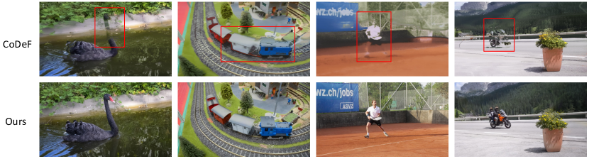
Figure 3: Visual comparison of reconstruction quality on the DAVIS [24] dataset. Based on explicit representation, 3DGS [10], our GFlow can recover dynamic scenes in high quality. In contrast, CoDeF [19], which is based on implicit representation, fails to model highly dynamic scenes. Better viewed by zooming in and in color.

Datasets

We conduct experiments on two challenging video datasets, DAVIS [24] and Tanks and Temples [11] to evaluate the video reconstruction quality and camera pose accuracy. While segmentation as a by-product, the object segmentation accuracy is also evulated. DAVIS dataset contains real-world videos of about 30~100 frames with various scenarios and motion dynamics. The salient object segmentation mask is labeled. We evaluate video reconstruction quality and object segmentation accuracy on DAVIS 2016 val dataset. Tanks and Temples [11] dataset contains videos with complex camera pose movement. And the corresponding camera poses are computed by COLMAP algorithm [26, 27]. Following [2], we evaluate camera pose accuracy on 8 scenes which cover both indoor and outdoor scenarios. We also evaluate video reconstruction quality on this dataset. Due to the long duration of videos in this dataset, we sample 1 frame every 4 frames for efficient evaluation.

Evaluation metrics

To quantitatively evaluation our GFlow’s capabilities, we adopt following metrics. For reconstruction quality, we report standard PSNR (Peak Signal-to-Noise Ratio), SSIM (Structural Similarity Index) and LPIPS [41] (Learned Perceptual Image Patch Similarity) metrics. As for camera pose accuracy, we report standard visual odometry metrics [29, 42], including the Absolute Trajectory Error (ATE) and Relative Pose Error (RPE) of rotation and translation as in [2, 14].

Implementation details

All image sequences are resized so that the shortest side is 480 pixels. The initial number of Gaussian points is set to 40,000. The camera intrinsics $K$ are averaged from the camera intrinsics of all frames predicted by DUSt3R [32]. We use two Adam optimizers for the two optimization procedures. The learning rate for Gaussian optimization is set to $1e\text{-}3$, and for camera optimization, it is set to $1e\text{-}4$. The number of optimization iterations is set to 500 for Gaussian optimization in the first frame, 150 for camera optimization, and 300 for Gaussian optimization in subsequent frames. The color gradient is set to zero, enforcing Gaussian points to move rather than lazily changing color. We balance the loss term by setting hyper-parameters $\lambda_{p}=1$, $\lambda_{d}=1e\text{-}4$, $\lambda_{s}=1$, and $\lambda_{f}=1e\text{-}2$. Densification is conducted at the 150-th and 300-th steps in the first frame optimization. For subsequent frames, the densification of Gaussian points occurs at the first step with a new content mask applied and at the 100-th step without any mask applied. The threshold $\tau$, portion $p_{1}$, portion $p_{2}$ in densification are set to $1e\text{-}2$, $20\%$ and $20\%$ respectively. All experiments are conducted on a single NVIDIA RTX A5000 GPU, taking tens of minutes per video. Unless otherwise specified, the experimental setup for evaluation is as mentioned above. Note that the dynamics within each video could be distinct, so for better reconstruction, the hyperparameters could be tuned in practice.

4.1 Evaluation results

4.1.1 Video reconstruction

Quantitative results

Reconstructing the 4D world, particularly with camera and content movement, is an extremely challenging task. As we are the first to address this problem, we choose CoDeF [19], the method closest to tackle this task, as our baseline. CoDeF employs implicit representation to learn a canonical template for modeling monocular video, which lacks physical interpretability, such as estimating camera pose. As shown in Table 1, our GFlow demonstrates significant advantages in reconstruction quality. This improvement stems from its explicit representation, which can adapt positions over time while maintaining visual content coherence.

Table 1: Reconstruction quality results on DAVIS[24] dataset. Average PSNR, SSIM and LPIPS scores on all videos are reported.

Method	DAVIS			Tanks and Temples
	PSNR$\uparrow$	SSIM$\uparrow$	LPIPS$\downarrow$	PSNR$\uparrow$	SSIM$\uparrow$	LPIPS$\downarrow$
CoDeF [19]	24.8904	0.7703	0.2932	26.8442	0.8160	0.1760
GFlow (Ours)	29.5508	0.9387	0.1067	32.7258	0.9720	0.0363
w/o scene clustering	26.3831	0.9032	0.1478	32.4098	0.9706	0.0387

Qualitative results

The visual comparison in Figure 3 shows that CoDeF [19] struggles to reconstruct videos with significant movement due to its reliance on representing a video as a canonical template. Since the essence of a canonical template is a 2D image, so CoDeF cannot handle complex spatial relationships and dynamic changes as effectively as our GFlow.

4.1.2 Object segmentation

Table 2: Object segmentation results on DAVIS[24] dataset. Region similarity ($\mathcal{J}$), contour accuracy ($\mathcal{F}$) and temporal stability ($\mathcal{T}$) [24] are reported. It is worth noting that our GFlow framework was not specifically trained for object segmentation; this capability emerges as a by-product. One-shot / zero-shot refers to whether the mask prompt of the first frame is given.

Method	One-shot			Zero-shot
	$\mathcal{J}\uparrow$	$\mathcal{F}\uparrow$	$\mathcal{J}\&\mathcal{F}\uparrow$	$\mathcal{J}\uparrow$	$\mathcal{F}\uparrow$	$\mathcal{J}\&\mathcal{F}\uparrow$
GFlow (Ours)	36.1	34.9	35.5	38.3	39.5	38.9
w/o scene clustering	15.1	11.6	13.4	-	-	-

Since GFlow drives the Gaussian points to follow the movement of the visual content, given an initial one-shot mask prompt, all Gaussian points within this mask can propagate to subsequent frames. This propagation forms a new mask as a concave hull [20] around these points. Notably, this capability is a by-product of GFlow, achieved without extra intended training. The evaluation results are shown in Table 2. Even without an initial mask prompt, GFlow can still generate high-quality zero-shot segmentation masks. These masks are produced based on the moving Gaussian points resulting from scene clustering in an unsupervised manner, as demonstrated in Figure 1.

4.1.3 Point tracking

The tracking trajectories are illustrated in Figure 4. Due to the nature of GFlow, all Gaussian points can serve as query tracking points, enabling tracking in both 2D and 3D coordinates. In conventional 2D tracking, the tracking occurs in the camera-view, which includes the joint motion of both the camera and the content. In contrast, the Gaussian points of GFlow reside in the 3D world-coordinates, representing only content movement. As a result, some 3D tracking trajectories tend to remain in their original locations, as shown in Figure 4 B), because they are part of the still background.

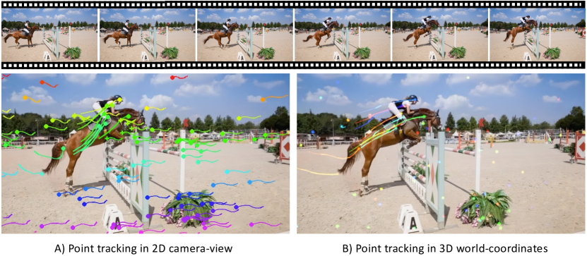
Figure 4: Point tracking visualization on DAVIS [24] dataset. A) shows tracking in the 2D camera-view which contains joint motion of camera and content movement. B) shows tracking in the 3D world-coordinates which only present content movement.

4.1.4 Camera pose estimation

Our method can reconstruct the 4D world along with corresponding camera poses. Since some components of GFlow are specifically designed for dynamic scenes, we slightly adjust the settings for evaluating camera pose accuracy on the Tanks and Temples dataset, which consists of static scenes. We modify the scene clustering procedure to treat all Gaussian points as static, as there’s no need to distinguish moving parts in a static scene. The results are shown in Table 3. As an on-the-fly optimization method, we achieve comparable results to global optimization methods that repeatedly observe each view, while requiring significantly less time.

Table 3: Camera pose estimation results on Tanks and Temples [11] dataset. Absolute trajectory error (ATE) and relative pose error (RPE) are reported. The unit of RPE_r is in degrees, ATE is in the ground truth scale and RPE_t is scaled by 100.

Method	Time$\downarrow$	$\textit{RPE}_{t}\downarrow$	$\textit{RPE}_{r}\downarrow$	$\textit{ATE}\downarrow$
Global Optimization
NoPe-NeRF [2]	~25 hrs	0.080	0.038	0.006
BARF [14]	-	1.046	0.441	0.078
NeRFmm [34]	-	1.735	0.477	0.123
On-the-fly Optimization
GFlow (Ours)	~15 mins	1.653	0.177	0.016

4.2 Ablation study

Effect of scene clustering

One of the biggest challenges in this task could be the dynamic nature of the scene, involving both content and camera movements. Therefore, as a key component of our framework, scene clustering plays a crucial role in distinguishing between moving and static parts. As can be seen from Table 1, without scene clustering, the framework degenerates to static scene reconstruction, compromising the reconstruction quality of dynamic scenes. Similarly, from Table 2, we observe negative influences on segmentation when scene clustering is not applied.

4.3 Downstream video applications

Various downstream applications could be extended from our GFlow framework. Since explicit representation can be easily edited: Camera-level manipulation: Changing the camera extrinsics can render novel views of dynamic scenes. When combined with camera intrinsics, it can create visual effects like dolly zoom. Object-level editing: With the cluster labels of moving Gaussian points, we can add, remove, resize, or stylize these points, allowing for precise object-level editing. Scene-level editing: Editing can also be applied to the entire scene, enabling the application of visual effects globally, as illustrated in Figure 1.

5 Related works

4D reconstruction from video, also known as dynamic 3D scene reconstruction, NeRFs [18] are implicit representations initially proposed for reconstructing static scenes. Subsequent works extended NeRFs to handle dynamic scenes [21, 22, 25, 13], typically using grids, triplanes [3, 5, 28], or learning deformable fields to map a canonical template [19, 9]. Although some efforts have accelerated the training speed of NeRFs [15, 23], achieving real-time rendering for dynamic scenes remains challenging, especially with monocular input.

Recent developments in 3D Gaussian Splatting (3DGS) [10] have set new records in rendering speed. Extensions of 3DGS [35, 17, 40, 39] have begun exploring dynamic scene reconstruction. However, they still operate under the assumption of a known camera sequence [27, 26].

While all these methods either rely on pre-calibrated camera parameters or multi-view video inputs to reconstruct dynamic scenes [35, 17, 30, 1, 3, 5, 12, 15, 16, 25], or estimate camera poses from static scenes using multi-view stereo techniques [2, 6, 32, 14, 34, 36, 27, 26, 31, 4]. The key difference between our GFlow and these approaches lies in our ability to perform dynamic scene reconstruction from a single, unposed monocular video.

6 Limitations

Although GFlow effectively reconstructs the 4D world from monocular unposed video and enables numerous applications, several key challenges remain: Our approach relies on off-the-shelf depth and optical flow components, where inaccuracies can compromise the precision and fidelity of our reconstruction. Specifically, inaccurate depth maps may lead to incorrect spatial placements of Gaussian points, while erroneous optical flow can result in improper motion estimation and dynamic scene representation. To address these issues, we could integrate more advanced multi-frame stereo methods to refine depth estimation and incorporate semantic features to better associate and track moving objects. Additionally, the current use of K-Means clustering for scene clustering may be inadequate for complex scenarios, suggesting the need for a more sophisticated and comprehensive clustering strategy. Furthermore, our on-the-fly online optimization can introduce and accumulate errors over time; thus, implementing a look-back or global optimization method could mitigate these accumulated errors and enhance overall accuracy. Addressing these challenges is crucial for improving the precision and robustness of GFlow in reconstructing dynamic 4D scenes.

7 Conclusion

We have presented "GFlow", a novel framework designed to address the challenging task of reconstructing the 4D world from monocular video inputs, termed "AnyV4D". Through scene clustering and sequential optimization of camera and Gaussian points, coupled with pixel-wise densification, GFlow enables the recovery of dynamic scenes alongside camera poses across frames. Further capabilities such as tracking, segmentation, editing, and novel view rendering, highlighting the potential for GFlow to revolutionize video understanding and manipulation.

References

- [1] Aayush Bansal, Minh Vo, Yaser Sheikh, Deva Ramanan, and Srinivasa Narasimhan. 4d visualization of dynamic events from unconstrained multi-view videos. In Proceedings of the IEEE/CVF Conference on Computer Vision and Pattern Recognition, pages 5366–5375, 2020.
- [2] Wenjing Bian, Zirui Wang, Kejie Li, Jia-Wang Bian, and Victor Adrian Prisacariu. Nope-nerf: Optimising neural radiance field with no pose prior. In Proceedings of the IEEE/CVF Conference on Computer Vision and Pattern Recognition, pages 4160–4169, 2023.
- [3] Ang Cao and Justin Johnson. Hexplane: A fast representation for dynamic scenes. In Proceedings of the IEEE/CVF Conference on Computer Vision and Pattern Recognition, pages 130–141, 2023.
- [4] David Charatan, Sizhe Li, Andrea Tagliasacchi, and Vincent Sitzmann. pixelsplat: 3d gaussian splats from image pairs for scalable generalizable 3d reconstruction. arXiv preprint arXiv:2312.12337, 2023.
- [5] Sara Fridovich-Keil, Giacomo Meanti, Frederik Rahbæk Warburg, Benjamin Recht, and Angjoo Kanazawa. K-planes: Explicit radiance fields in space, time, and appearance. In Proceedings of the IEEE/CVF Conference on Computer Vision and Pattern Recognition, pages 12479–12488, 2023.
- [6] Yang Fu, Sifei Liu, Amey Kulkarni, Jan Kautz, Alexei A Efros, and Xiaolong Wang. Colmap-free 3d gaussian splatting. arXiv preprint arXiv:2312.07504, 2023.
- [7] John A Hartigan and Manchek A Wong. Algorithm as 136: A k-means clustering algorithm. Journal of the royal statistical society. series c (applied statistics), 28(1):100–108, 1979.
- [8] Nick Kanopoulos, Nagesh Vasanthavada, and Robert L Baker. Design of an image edge detection filter using the sobel operator. IEEE Journal of solid-state circuits, 23(2):358–367, 1988.
- [9] Yoni Kasten, Dolev Ofri, Oliver Wang, and Tali Dekel. Layered neural atlases for consistent video editing. ACM Transactions on Graphics (TOG), 40(6):1–12, 2021.
- [10] Bernhard Kerbl, Georgios Kopanas, Thomas Leimkühler, and George Drettakis. 3d gaussian splatting for real-time radiance field rendering. ACM Transactions on Graphics, 42(4):1–14, 2023.
- [11] Arno Knapitsch, Jaesik Park, Qian-Yi Zhou, and Vladlen Koltun. Tanks and temples: Benchmarking large-scale scene reconstruction. ACM Transactions on Graphics (ToG), 36(4):1–13, 2017.
- [12] Tianye Li, Mira Slavcheva, Michael Zollhoefer, Simon Green, Christoph Lassner, Changil Kim, Tanner Schmidt, Steven Lovegrove, Michael Goesele, Richard Newcombe, et al. Neural 3d video synthesis from multi-view video. In Proceedings of the IEEE/CVF Conference on Computer Vision and Pattern Recognition, pages 5521–5531, 2022.
- [13] Zhengqi Li, Qianqian Wang, Forrester Cole, Richard Tucker, and Noah Snavely. Dynibar: Neural dynamic image-based rendering. In Proceedings of the IEEE/CVF Conference on Computer Vision and Pattern Recognition, pages 4273–4284, 2023.
- [14] Chen-Hsuan Lin, Wei-Chiu Ma, Antonio Torralba, and Simon Lucey. Barf: Bundle-adjusting neural radiance fields. In Proceedings of the IEEE/CVF International Conference on Computer Vision, pages 5741–5751, 2021.
- [15] Haotong Lin, Sida Peng, Zhen Xu, Tao Xie, Xingyi He, Hujun Bao, and Xiaowei Zhou. High-fidelity and real-time novel view synthesis for dynamic scenes. In SIGGRAPH Asia 2023 Conference Papers, pages 1–9, 2023.
- [16] Kai-En Lin, Lei Xiao, Feng Liu, Guowei Yang, and Ravi Ramamoorthi. Deep 3d mask volume for view synthesis of dynamic scenes. In Proceedings of the IEEE/CVF International Conference on Computer Vision, pages 1749–1758, 2021.
- [17] Jonathon Luiten, Georgios Kopanas, Bastian Leibe, and Deva Ramanan. Dynamic 3d gaussians: Tracking by persistent dynamic view synthesis. arXiv preprint arXiv:2308.09713, 2023.
- [18] Ben Mildenhall, Pratul P Srinivasan, Matthew Tancik, Jonathan T Barron, Ravi Ramamoorthi, and Ren Ng. Nerf: Representing scenes as neural radiance fields for view synthesis. Communications of the ACM, 65(1):99–106, 2021.
- [19] Hao Ouyang, Qiuyu Wang, Yuxi Xiao, Qingyan Bai, Juntao Zhang, Kecheng Zheng, Xiaowei Zhou, Qifeng Chen, and Yujun Shen. Codef: Content deformation fields for temporally consistent video processing. arXiv preprint arXiv:2308.07926, 2023.
- [20] Jin-Seo Park and Se-Jong Oh. A new concave hull algorithm and concaveness measure for n-dimensional datasets. Journal of Information science and engineering, 28(3):587–600, 2012.
- [21] Keunhong Park, Utkarsh Sinha, Jonathan T Barron, Sofien Bouaziz, Dan B Goldman, Steven M Seitz, and Ricardo Martin-Brualla. Nerfies: Deformable neural radiance fields. In Proceedings of the IEEE/CVF International Conference on Computer Vision, pages 5865–5874, 2021.
- [22] Keunhong Park, Utkarsh Sinha, Peter Hedman, Jonathan T Barron, Sofien Bouaziz, Dan B Goldman, Ricardo Martin-Brualla, and Steven M Seitz. Hypernerf: A higher-dimensional representation for topologically varying neural radiance fields. arXiv preprint arXiv:2106.13228, 2021.
- [23] Sida Peng, Yunzhi Yan, Qing Shuai, Hujun Bao, and Xiaowei Zhou. Representing volumetric videos as dynamic mlp maps. In Proceedings of the IEEE/CVF Conference on Computer Vision and Pattern Recognition, pages 4252–4262, 2023.
- [24] Federico Perazzi, Jordi Pont-Tuset, Brian McWilliams, Luc Van Gool, Markus Gross, and Alexander Sorkine-Hornung. A benchmark dataset and evaluation methodology for video object segmentation. In Proceedings of the IEEE conference on computer vision and pattern recognition, pages 724–732, 2016.
- [25] Albert Pumarola, Enric Corona, Gerard Pons-Moll, and Francesc Moreno-Noguer. D-nerf: Neural radiance fields for dynamic scenes. In Proceedings of the IEEE/CVF Conference on Computer Vision and Pattern Recognition, pages 10318–10327, 2021.
- [26] Johannes L Schonberger and Jan-Michael Frahm. Structure-from-motion revisited. In Proceedings of the IEEE conference on computer vision and pattern recognition, pages 4104–4113, 2016.
- [27] Johannes L Schönberger, Enliang Zheng, Jan-Michael Frahm, and Marc Pollefeys. Pixelwise view selection for unstructured multi-view stereo. In Computer Vision–ECCV 2016: 14th European Conference, Amsterdam, The Netherlands, October 11-14, 2016, Proceedings, Part III 14, pages 501–518. Springer, 2016.
- [28] Ruizhi Shao, Zerong Zheng, Hanzhang Tu, Boning Liu, Hongwen Zhang, and Yebin Liu. Tensor4d: Efficient neural 4d decomposition for high-fidelity dynamic reconstruction and rendering. In Proceedings of the IEEE/CVF Conference on Computer Vision and Pattern Recognition, pages 16632–16642, 2023.
- [29] Jürgen Sturm, Nikolas Engelhard, Felix Endres, Wolfram Burgard, and Daniel Cremers. A benchmark for the evaluation of rgb-d slam systems. In 2012 IEEE/RSJ international conference on intelligent robots and systems, pages 573–580. IEEE, 2012.
- [30] Jiakai Sun, Han Jiao, Guangyuan Li, Zhanjie Zhang, Lei Zhao, and Wei Xing. 3dgstream: On-the-fly training of 3d gaussians for efficient streaming of photo-realistic free-viewpoint videos. arXiv preprint arXiv:2403.01444, 2024.
- [31] Fengrui Tian, Shaoyi Du, and Yueqi Duan. Mononerf: Learning a generalizable dynamic radiance field from monocular videos. In Proceedings of the IEEE/CVF International Conference on Computer Vision, pages 17903–17913, 2023.
- [32] Shuzhe Wang, Vincent Leroy, Yohann Cabon, Boris Chidlovskii, and Jerome Revaud. Dust3r: Geometric 3d vision made easy. arXiv preprint arXiv:2312.14132, 2023.
- [33] Zhou Wang, Alan C Bovik, Hamid R Sheikh, and Eero P Simoncelli. Image quality assessment: from error visibility to structural similarity. IEEE transactions on image processing, 13(4):600–612, 2004.
- [34] Zirui Wang, Shangzhe Wu, Weidi Xie, Min Chen, and Victor Adrian Prisacariu. Nerf–: Neural radiance fields without known camera parameters. arXiv preprint arXiv:2102.07064, 2021.
- [35] Guanjun Wu, Taoran Yi, Jiemin Fang, Lingxi Xie, Xiaopeng Zhang, Wei Wei, Wenyu Liu, Qi Tian, and Xinggang Wang. 4d gaussian splatting for real-time dynamic scene rendering. arXiv preprint arXiv:2310.08528, 2023.
- [36] Yitong Xia, Hao Tang, Radu Timofte, and Luc Van Gool. Sinerf: Sinusoidal neural radiance fields for joint pose estimation and scene reconstruction. arXiv preprint arXiv:2210.04553, 2022.
- [37] Haofei Xu, Jing Zhang, Jianfei Cai, Hamid Rezatofighi, and Dacheng Tao. Gmflow: Learning optical flow via global matching. In Proceedings of the IEEE/CVF conference on computer vision and pattern recognition, pages 8121–8130, 2022.
- [38] Haofei Xu, Jing Zhang, Jianfei Cai, Hamid Rezatofighi, Fisher Yu, Dacheng Tao, and Andreas Geiger. Unifying flow, stereo and depth estimation. IEEE Transactions on Pattern Analysis and Machine Intelligence, 2023.
- [39] Zeyu Yang, Hongye Yang, Zijie Pan, Xiatian Zhu, and Li Zhang. Real-time photorealistic dynamic scene representation and rendering with 4d gaussian splatting. arXiv preprint arXiv:2310.10642, 2023.
- [40] Ziyi Yang, Xinyu Gao, Wen Zhou, Shaohui Jiao, Yuqing Zhang, and Xiaogang Jin. Deformable 3d gaussians for high-fidelity monocular dynamic scene reconstruction. arXiv preprint arXiv:2309.13101, 2023.
- [41] Richard Zhang, Phillip Isola, Alexei A Efros, Eli Shechtman, and Oliver Wang. The unreasonable effectiveness of deep features as a perceptual metric. In CVPR, 2018.
- [42] Zichao Zhang and Davide Scaramuzza. A tutorial on quantitative trajectory evaluation for visual (-inertial) odometry. In 2018 IEEE/RSJ International Conference on Intelligent Robots and Systems (IROS), pages 7244–7251. IEEE, 2018.