RealTimeTransport: An open-source C++ library for quantum transport simulations in the strong coupling regime

Abstract

The description of quantum transport in the strong system-reservoir coupling regime poses a significant theoretical and computational challenge that demands specialized tools for accurate analysis. RealTimeTransport is a new open-source C++ library that enables the computation of both stationary and transient transport observables for generic quantum systems connected to metallic reservoirs. It computes the Nakajima-Zwanzig memory kernels for both dynamics and transport in real-time going beyond traditional expansions in the bare system-reservoir couplings. Currently, several methods are available: (i) A renormalized perturbation theory in leading and next-to-leading order which avoids the low-temperature breakdown that limits the traditional theory. (ii) Starting from this well-behaved reference solution a 2- and 3-loop self-consistent renormalization-group transformation of the memory kernels is implemented. This allows refined quantitative predictions even in the presence of many body resonances, such as the Kondo enhancement of cotunneling. This paper provides an overview of the theory, the architecture of RealTimeTransport and practical demonstrations of the currently implemented methods. In particular, we analyze the stationary transport through a serial double quantum dot and showcase for the $T=0$ interacting Anderson model the complete time-development of single-electron tunneling (SET), cotunneling-assisted SET (CO-SET) and inelastic cotunneling resonances throughout the entire gate-bias stability diagram. We discuss the range of applicability of the implemented methods and benchmark them against other advanced approaches.

I Introduction

The accurate description of quantum transport phenomena is fundamental to the understanding of quantum dot devices. These are interesting platforms to study fundamental aspects of open quantum systems, featuring a rich interplay of non-equilibrium physics and many-body effects, as well as for various (quantum) technologies. CODE(0x6545b244c318)hough their stationary transport properties are by now fairly well-understood, their dynamical aspects remain challenging.

From a methodological perspective an accurate description in extended parameter regimes is challenging. Non-equilibrium Green’s function methods are well-suited to study systems at low temperature, but struggle to treat strong Coulomb interactions which are typically incorporated perturbatively or in mean-field approximation. CODE(0x6545b244c318)s has been improved by various means, in particular by applying renormalization group (RG) methods within this framework. CODE(0x6545b244c318)he other hand, a plethora of quantum master equation (QME) approaches exist, CODE(0x6545b244c318)ch treat the quantum dot energy scales non-perturbatively. These instead assume that the system-reservoir coupling is weak, which prohibits their usage at temperatures below the energy scale set by the tunnel rate. Just like Green’s function approaches, master equation-like methods can be improved by applying RG ideas, but in this case to approach stronger system-reservoir couplings and lower temperatures. CODE(0x6545b244c318) above mentioned methods are semi-analytical, which often aids the understanding of the results, and the work reported here follows this line. Fully numerical approaches such as scattering state numerical renormalization groups, CODE(0x6545b244c318)me-dependent) density matrix renormalization groups CODE(0x6545b244c318)uantum monte carlo methods CODE(0x6545b244c318)st to name a few, have also been successfully applied.

In this paper we present RealTimeTransport, a C++ library which implements several methods to analyze both transient and stationary quantum transport quantities based on the Nakajima-Zwanzig memory kernel of the open system.  As the name suggests, the package is consistently based on the time-domain representation of the dynamics and transport. It thereby maintains a useful connection to the intuition of traditional quantum master equations (QMEs): inside the “black box” one can still identify rates for state transitions and Bloch coherence-vector dynamics. At the same time it fixes shortcomings of these QMEs by fully accounting for renormalization and memory effects. Key technical steps of our approach were heavily inspired by the so-called “$E$-flow” RG formulated in frequency domain ($E$), which was successfully used to analytically and numerically describe the non-equilibrium Kondo effect in the stationary and time-dependent case. CODE(0x6545b244c318)nstead remain in the time domain noting that there the memory kernel is typically well-behaved and can be efficiently resolved using well-developed Chebyshev interpolation techniques. CODE(0x6545b244c318)

Roughly speaking our approach works as follows: In ordinary bare perturbation theory one initially eliminates all dissipation from the problem by setting the coupling to the reservoir to zero. One then computes the corrections to this “too small dissipation” to increase it. In our approach we do exactly the opposite: We initially analytically solve the problem in the physical limit of infinite temperature leading to “too large dissipation” and then compute corrections to this. In prior work this was done by a “$T$-flow” from infinitely high temperature to the low temperature of interest. CODE(0x6545b244c318)s involved solving a differential RG equation with respect to the physical temperature $T$, which at low $T$ approaches a fixed point (in the space of time-dependent memory kernels and vertex functions).

In the present work we perform this computation in a new way. We exploit that the “too large dissipation” computed at $T=\infty$ allows to construct an ansatz which is well-behaved even at $T=0$. This reference solution incorporates all $T=\infty$ effects and is the leading term of a much simplified renormalized perturbation series. In particular, this ansatz is very similar to the bare perturbation expression whose virtual intermediate evolutions are regularized as $i0^{+}\to\Sigma_{\infty}$, i.e., by replacing the problematic zero-dissipation by the $T=\infty$ Lindblad generator. Importantly, this superoperator-valued regularization is systematically derived from a physical limit and not put in “by hand”. Our main result is that from this ansatz one can initiate a discrete RG iteration which converges stepwise to the same fixed point as the previous continuous $T$-flow, thus reducing the “too large dissipation” to the desired correct value. Importantly, for the low temperature of interest this discrete iteration turns out to be more efficient then the continous $T$-flow.

Although the RG aspects of the outlined method make it stand out, it is firmly routed in the well-developed line of quantum master equation approaches for which various numerical packages have been published. For example, the QuTiP (Quantum Toolbox in Python) package CODE(0x6545b244c318)lements phenomenological and leading order approaches in the system-reservoir coupling, such as the Lindblad, Bloch-Redfield and Floquet-Markov QMEs. QmeQ (Quantum master equations for Quantum dot transport calculations) CODE(0x6545b244c318)o implements several leading order methods, but additionally provides next-to-leading order approximations of the stationary state and particle/energy current through a consistent expansion of the memory kernel or the second-order von Neumann approach.

The paper is structured as follows: In Sec. II we first present the time-space perturbation theory for the memory kernel of the density operator and then develop the above mentioned renormalized version of this. Based on this we set up the new discrete iterative RG transformation and comment on some implementation details in Sec. III. In Sec. IV we then showcase the practical library usage for several examples. In particular, we analyze the stationary transport through a serial double quantum dot and present the time evolution of the non-equilibrium interacting Anderson model in a magnetic field at zero temperature. This showcases the emergence of different strongly-correlated phenomena at distinct time-scales which is mapped out for all applied bias and gate voltages. We note that the stationary limit of this problem has by now been experimentally probed in detail in many types of quantum dots, ranging from semi-conductor heterostructures, carbon-based materials to molecular and atomic quantum dots. CODE(0x6545b244c318)ally, we benchmark our methods against the density matrix renormalization group and quantum Monte Carlo approach.

II Computation of the memory kernel

In the following we set $\hbar=k_{B}=e=1$.

II.1 Model and notation

We consider a quantum dot system connected to several non-interacting electron reservoirs in the thermodynamic limit. Each of the reservoirs labeled by $r$ is assumed to be initially in a grand canonical equilibrium with temperature $T_{r}$ and chemical potential $\mu_{r}$. Thus the Hamiltonian describing the isolated reservoirs is given by

$$H_{R}=\sum_{r\nu}\int d\omega(\omega+\mu_{r})a^{\dagger}_{r\nu}(\omega)a_{r\nu}(\omega),$$ (1)

and the initial state of the reservoirs is

$$\rho_{R}=\prod_{r}\frac{1}{Z_{r}}e^{-\beta_{r}\sum_{\nu}\int d\omega\omega a^{\dagger}_{r\nu}(\omega)a_{r\nu}(\omega)}.$$ (2)

Here $\nu$ denotes a generic channel index of the reservoirs, which is often just the spin $\sigma$. The field operators $a^{\dagger}_{r\nu}$ ($a_{r\nu}$) create (destroy) an electron with channel index $\nu$ in reservoir $r$ and anti-commute as

$$\big{\{}a_{r\nu}(\omega),a^{\dagger}_{r^{\prime}\nu^{\prime}}(\omega^{\prime})\big{\}} =\delta_{rr^{\prime}}\delta_{\nu\nu^{\prime}}\delta(\omega-\omega^{\prime}),$$ (3a)

$$\big{\{}a_{r\nu}(\omega),a_{r^{\prime}\nu^{\prime}}(\omega^{\prime})\big{\}} =0.$$ (3b)

It is useful to introduce an additional particle-hole index $\eta$ and define

$$a_{\eta r\nu\omega} \coloneqq\left\{\begin{array}[]{lrl}a^{\dagger}_{r\nu}(\omega)&\text{for}&\eta=+\\ a_{r\nu}(\omega)&\text{for}&\eta=-\end{array}\right..$$ (6)

For notational convenience we collect all indices into a multi-index written as a number,

$$1\equiv\eta,r,\nu,\omega;\quad\bar{1}\equiv-\eta,r,\nu,\omega,$$ (7)

where the overbar indicates the inversion of the particle-hole index. This allows us to rewrite the anti-commutation relations (3) compactly as

$$\{a_{1},a_{2}\}=\delta_{1\bar{2}}.$$ (8)

Electrons can tunnel between the reservoirs and quantum dot system, which is captured by the tunneling Hamiltonian

$$H_{T}=\sum_{r\nu l}\int d\omega\sqrt{\lambda_{r\nu}}t_{r\nu l}d^{\dagger}_{l}a_{r\nu}(\omega)+\text{h.c.}$$ (9)

Here $d_{l}$ denotes a field operator of the quantum dot system and $l$ a (multi)index labeling the single particle states, including the spin and orbital quantum numbers. Importantly, the Fock space can always be constructed such that the field operators $d_{l}$ of the system and $a_{r\nu}(\omega)$ of the reservoir commute, rather than anti-commute. This is explained in Sec. II. A. of Ref. [Saptsov and Wegewijs, 2014]: one transforms from the conventional anti-commutation to commutation using the fermion parity operators of the system and reservoir, respectively. This is crucial for tracing out the fermionic reservoir degrees of freedom later on, because it avoids keeping track of various minus signs.

We assume that the density of states $\lambda_{r\nu}$ and tunneling amplitudes $t_{r\nu l}$ are energy independent (wideband limit) and real-valued. They will later enter the transport equations via the spectral density, which we define as

$$\Gamma_{rll^{\prime}}\coloneqq 2\pi\sum_{\nu}\lambda_{r\nu}t_{r\nu l}t_{r\nu l^{\prime}}.$$ (10)

The Hamiltonian $H$ describing the isolated quantum dot system is only constrained by the assumption that it should commute with the fermion parity (as any physical Hamiltonian should). CODE(0x6545b244c318)s is because the fermion parity superselection principle is explicitly incorporated into the superfermionic perturbation theory introduced later. Thus, the total Hamiltonian we consider is given by

$$H_{\text{tot}}=H+H_{R}+H_{T}.$$ (11)

II.2 Superfermionic perturbation theory

For initial total states that factorize, $\rho^{0}_{\text{tot}}=\rho_{0}\otimes\rho_{R}$, the dynamics of the reduced density operator $\rho(t)\coloneqq\operatorname{Tr}_{R}\rho_{\text{tot}}(t)$ can be described using the superoperator-valued propagator $\Pi(t)$ as $\rho(t)=\Pi(t)\rho_{0}$. The dynamics of $\Pi(t)$ follows the time-nonlocal Nakajima-Zwanzig quantum master equation, CODE(0x6545b244c318)Π(t) = -i LΠ(t) - i ∫_0^t ds K(t-s) Π(s), where $\mathcal{L}\bullet=[H,\bullet]$ denotes the bare Liouvillian, $\mathcal{K}$ the memory kernel and the bullet an arbitrary operator argument. Our main goal is to compute the memory kernel $\mathcal{K}$. The perturbative expansion of $\mathcal{K}$ in the system-environment coupling is well-established, CODE(0x6545b244c318) most commonly done in frequency space and in particular done at $\omega=0$, where the stationary state can be extracted. However, in order to implement the renormalization group transformation presented in Sec. II.4, it is necessary to resolve the memory kernel either for all frequencies or alternatively for all times. Because the memory kernel as a function of time is typically well behaved and (at finite temperatures) exponentially decaying, it can be efficiently interpolated using Chebyshev polynomials, CODE(0x6545b244c318)ch is done within RealTimeTransport. We will therefore outline the main steps to derive a time-space perturbation theory for $\mathcal{K}$ using the superfermionic formulation as presented in detail in Refs. [Saptsov and Wegewijs, 2012, 2014]. This formulation is also at the heart of the more powerful methods presented in the subsequent sections. The crucial starting point is the definition of superfield operators as

$$J^{p}_{1}\bullet\coloneqq\frac{1}{\sqrt{2}}\,\Big{[}a_{1}\bullet+p(-\mathds{1})^{n_{R}}\bullet(-\mathds{1})^{n_{R}}a_{1}\Big{]},$$ (12)

where $(-\mathds{1})^{n_{R}}$ denotes the fermion parity of the reservoirs. These superfields are called superfermions, because they act analogously to ordinary field operators $a_{1}$ in Liouville space. For example, they anticommute as

$$\left\{J_{1}^{p_{1}},J_{2}^{p_{2}}\right\}=\delta_{p_{1}\bar{p}_{2}}\delta_{1\bar{2}}$$ (13)

and obey a super-Pauli principle $(J^{p}_{1})^{2}=0$. CODE(0x6545b244c318)s, $J^{+}_{1}$ ($J^{-}_{1}$) can be thought of as creating (annihilating) an excitation in Liouville space. By defining similar superfermions in the quantum dot systems Liouville space,

$$D^{p}_{1}\bullet\coloneqq\frac{1}{\sqrt{2}}\,\Big{[}d_{1}\bullet+p(-\mathds{1})^{n}\bullet(-\mathds{1})^{n}d_{1}\Big{]},$$ (14)

we can express the tunneling Liouvillian $\mathcal{L}_{T}\coloneqq[H_{T},\bullet]$ as

$$\mathcal{L}_{T}=\sqrt{\lambda_{1}}t_{1}D_{1}^{p}J_{\bar{1}}^{\bar{p}}.$$ (15)

Here $\bar{p}\coloneqq-p$ and we implicitly sum/integrate over $p$ and $1=\eta,l,r,\nu,\omega$. Note that in writing Eq. (15) we explicitly used the fermion parity superselection principle $(-\mathds{1})^{n_{\text{tot}}}\rho_{\text{tot}}(-\mathds{1})^{n_{\text{tot}}}=\rho_{\text{tot}}$, where $(-\mathds{1})^{n_{\text{tot}}}$ denotes the fermion parity of the total system and $\rho_{\text{tot}}$ any physical state. CODE(0x6545b244c318)fining the unperturbed propagators of the dot and reservoir as $\Pi_{0}(t)\coloneqq e^{-i\mathcal{L}t}$ and $\Pi_{R}(t)\coloneqq e^{-i\mathcal{L}_{R}t}$ respectively, we can expand the full propagator $\Pi$ in orders of the tunneling Liouvillian $\mathcal{L}_{T}$. By implicitly summing over $n\in\mathbbm{N}_{0}$ and integrating over all intermediate times $\tau_{i}$ in a time-ordered fashion $t\geq\tau_{1}\geq\dots\geq\tau_{n}\geq 0$ we obtain

$$\Pi(t)= (-i)^{n}\big{\langle}\Pi_{0R}(t-\tau_{1})\mathcal{L}_{T}\dots\mathcal{L}_{T}\Pi_{0R}(\tau_{n})\big{\rangle}_{R}$$ (16)

$$= (-i)^{n}\sqrt{\lambda_{1}}t_{1}\dots\sqrt{\lambda_{n}}t_{n}\Pi_{0}(t-\tau_{1})D_{1}^{p_{1}}\dots D_{n}^{p_{n}}\Pi_{0}(\tau_{n})$$

$$\times\big{\langle}\Pi_{R}(t-\tau_{1})J_{\bar{1}}^{\bar{p}_{1}}\Pi_{R}(\tau_{1}-\tau_{2})\dots J_{\bar{n}}^{\bar{p}_{n}}\Pi_{R}(\tau_{n})\big{\rangle}_{R}.$$ (17)

In (16) we used the shorthand notation $\Pi_{0R}=\Pi_{0}\Pi_{R}$ and $\langle\dots\rangle_{R}\coloneqq\operatorname{Tr}_{R}(\dots)\rho_{R}$. In (17) we inserted (15) and used that by construction all system superoperators commute with those of the reservoir, allowing us to pull all of them to the left. The last line of Eq. (17) only involves reservoir fields and can be evaluated using a superoperator version of Wick’s theorem, CODE(0x6545b244c318)ch decomposes the $n$-point expectation value $\langle J_{1}^{p_{1}}\dots J_{n}^{p_{n}}\rangle_{R}$ into sums of products of two-point expectation values $\langle J_{1}^{p_{1}}J_{2}^{p_{2}}\rangle_{R}$. A key simplification achieved by the superfermions (12) is that out of the four two-point expectation values one obtains by setting $p_{1/2}=\pm$, only two are non-zero. These are given by

$$\langle J_{1}^{-}J_{2}^{+}\rangle_{R} =\delta_{1\bar{2}},$$ (18a)

$$\langle J_{1}^{-}J_{2}^{-}\rangle_{R} =\delta_{1\bar{2}}\tanh\left(\frac{\eta_{2}\beta_{r_{2}}\omega_{2}}{2}\right).$$ (18b)

The internal $\omega_{i}$ integrations within Eq. (17) can then be incorporated into time-space contraction functions defined by

$$\gamma_{\eta_{1}l_{1},\eta_{2}l_{2}}^{p}(\tau)\coloneqq\sqrt{\lambda_{1}\lambda_{2}}t_{1}t_{2}\langle J_{\bar{1}}^{-}J_{\bar{2}}^{p}\rangle_{R}e^{-i\eta_{1}(\omega_{1}+\mu_{r_{1}})\tau},$$ (19)

where we again implicitly sum/integrate over all indices on the right hand side which do not occur on the left hand side. Evaluating the frequency integrals we obtain

$$\gamma_{\eta_{1}l_{1},\eta_{2}l_{2}}^{+}(\tau) =\delta_{\eta_{1}\bar{\eta}_{2}}\tfrac{1}{2}\sum_{r}\Gamma_{rl_{1}l_{2}}\bar{\delta}(\tau),$$ (20a)

$$\gamma_{\eta_{1}l_{1},\eta_{2}l_{2}}^{-}(\tau) =\delta_{\eta_{1}\bar{\eta}_{2}}\sum_{r}\frac{-i\Gamma_{rl_{1}l_{2}}T_{r}}{\sinh(\pi T_{r}\tau)}e^{-i\eta_{1}\mu_{r}\tau}.$$ (20b)

The $\bar{\delta}$ distribution occurring in $\gamma^{+}$ – defined as $\int_{0}^{t}\bar{\delta}(t-s)f(s)ds=f(t)$ – stems from the wideband limit taken in the definition of the tunneling Hamiltonian (9). Thus, we obtain the series expansion of the propagator in orders of the system-environment coupling, in a form where all reservoir degrees of freedom have been integrated out:

$$\Pi(t)= (-i)^{n}\sum_{\text{contr.}}(-1)^{N_{p}}\big{(}\prod_{\text{pairs $i<j$}}\delta_{p_{i}+}\gamma_{ij}^{\bar{p}_{j}}(\tau_{i}-\tau_{j})\big{)}$$

$$\times\Pi_{0}(t-\tau_{1})D_{1}^{p_{1}}\Pi_{0}(\tau_{1}-\tau_{2})\dots D_{n}^{p_{n}}\Pi_{0}(\tau_{n}).$$ (21)

Each term in Eq. (21) can be represented by a diagram, where vertices (superfermions), drawn as bullets, interrupt the bare evolutions $\Pi_{0}$ and are contracted in pairs. The memory kernel $\mathcal{K}$ is then given by the sum of all connected diagrams without legs, i.e., without the leftmost and rightmost bare propagator,

$$\mathcal{K}(t)= (-i)^{n}\sum_{\text{connected}}(-1)^{N_{p}}\big{(}\prod_{\text{pairs $i<j$}}\delta_{p_{i}+}\gamma_{ij}^{\bar{p}_{j}}(\tau_{i}-\tau_{j})\big{)}$$

$$\times D_{1}^{p_{1}}\Pi_{0}(t-\tau_{1})D_{2}^{p_{2}}\dots\Pi_{0}(\tau_{n-2})D_{n}^{p_{n}},$$ (22)

see the next section for examples. The factor $(-1)^{N_{p}}$ refers to the Wick-contraction sign, which is given by the number of crossings of contraction functions.

II.3 Renormalized perturbation theory around the infinite-temperature limit

The $\bar{\delta}$-function inside the memory kernel leads to a time-local contribution,

$$\mathcal{K}(t-s)=\Sigma_{\infty}\bar{\delta}(t-s)+\Sigma(t-s),$$ (23)

where

$$\Sigma_{\infty}\coloneqq-\frac{i}{2}\sum_{\eta rll^{\prime}}\Gamma_{rll^{\prime}}D^{+}_{\eta l}D^{-}_{\bar{\eta}l^{\prime}}.$$ (24)

Since the $\gamma^{-}$ contraction function (20b) vanishes if all $T_{r}\rightarrow\infty$, we can infer that the Liouvillian

$$L_{\infty}\coloneqq L+\Sigma_{\infty}$$ (25)

generates the exact semigroup dynamics at infinite temperature:

$$\Pi_{\infty}(t)\coloneqq\lim_{T_{r}\rightarrow\infty}\Pi(t)=e^{-iL_{\infty}t}.$$ (26)

This infinite temperature solution can be used as a new reference in a renormalized perturbation series. The key technical step is to realize that two vertices connected by a $\gamma^{+}$ contraction can never have any other vertices between them, due to vanishing support of the intermediate time integrations, which enables the resummation of all $\gamma^{+}$ contractions into $\Pi_{\infty}$ propagators (see Ref. [Saptsov and Wegewijs, 2014] for details). It is now easy to obtain the rules of the renormalized perturbation theory, for which one has to adapt those of the bare one as follows: (i) only creation superfermions $D^{+}_{1}$ and $\gamma^{-}_{1}$ contractions are allowed and (ii) every bare Liouvillian $\mathcal{L}$ must be renormalized as $\mathcal{L}\rightarrow\mathcal{L}_{\infty}$, which includes replacing bare propagators as $\Pi_{0}\rightarrow\Pi_{\infty}$. RealTimeTransport implements the leading and next-to-leading order of this renormalized perturbation theory. In leading order, the renormalized memory kernel is explicitly given by

$$-i\Sigma^{(1)}(t)=\raisebox{-0.3pt}{\includegraphics[height=12.80365pt]{diagrams/memory_kernel_1.pdf}}=-\gamma^{-}_{12}(t)D_{1}^{+}\Pi_{\infty}(t)D_{2}^{+}.$$ (27)

It is instructive to analyze the worst case $T\rightarrow 0$, where the bare perturbation theory suffers from a complete breakdown due to the very slow and oscillatory decay of the contraction function $\gamma^{-}(t)\propto e^{-i\eta_{1}\mu_{r}t}/t$. CODE(0x6545b244c318)ontrast, the limit $T\rightarrow 0$ is unproblematic in Eq. (27) because the intermediate renormalized propagator is still exponentially decaying towards the infinte-temperature stationary state $\Pi_{\infty}(t)\rightarrow\tfrac{1}{d}\bm{|}\mathds{1}\bm{)}\bm{(}\mathds{1}\bm{|}$, which is a left zero eigenvector of the $D^{+}_{2}$ creation superfermion on the right. CODE(0x6545b244c318)e next-to-leading order corrections are

$$-i\Sigma^{(2)}=\raisebox{-0.3pt}{\includegraphics[height=12.80365pt]{diagrams/memory_kernel_2.pdf}}+\raisebox{-0.3pt}{\includegraphics[height=12.80365pt]{diagrams/memory_kernel_3.pdf}},$$ (28)

where the diagrams are given by

$$\raisebox{-0.3pt}{\includegraphics[height=12.80365pt]{diagrams/memory_kernel_2.pdf}}= \gamma^{-}_{14}(t)\gamma^{-}_{23}(\tau_{1}-\tau_{2})D^{+}_{1}\Pi_{\infty}(t-\tau_{1})D^{+}_{2}$$

$$\times\Pi_{\infty}(\tau_{1}-\tau_{2})D^{+}_{3}\Pi_{\infty}(\tau_{2})D^{+}_{4},$$ (29)

$$\raisebox{-0.3pt}{\includegraphics[height=12.80365pt]{diagrams/memory_kernel_3.pdf}}= -\gamma^{-}_{13}(t-\tau_{2})\gamma^{-}_{24}(\tau_{1})D^{+}_{1}\Pi_{\infty}(t-\tau_{1})D^{+}_{2}$$

$$\times\Pi_{\infty}(\tau_{1}-\tau_{2})D^{+}_{3}\Pi_{\infty}(\tau_{2})D^{+}_{4}.$$ (30)

Here we again integrate in a time-ordered fashion over all intermediate times $\tau_{i}$, i.e., $t\geq\tau_{1}\geq\tau_{2}\geq 0$, and sum over all occuring multi-indices. Importantly, the singularities of $\gamma^{-}_{ij}(\tau)$ at $\tau=0$ within Eqs. (27)–(30) never contribute due to the algebra of the superfermions, which was shown in detail in App. A of Ref. [Nestmann and Wegewijs, 2021]. However, they need to be implemented carefully in order to not cause numerical problems. Finally, we mention that for non-interacting systems it can be shown that the renormalized perturbation theory terminates due to the super-Pauli principle. CODE(0x6545b244c318)cifically, for these systems the renormalized perturbation theory of order $n_{l}$ is exact, where $n_{l}$ denotes the number of single particle states. For example, this means that for a single spinful level (without interactions) Eqs. (27)–(30) give the exact memory kernel.

II.4 Renormalization group transformation

We now follow Ref. [Nestmann and Wegewijs, 2022] to derive a renormalization group transformation with a fixed point given by the time-dependent memory kernel $\Sigma$ [Eq. (23)]. Firstly, in each diagram we resum all connected subblocks without uncontracted lines to full propagators $\Pi$, which we draw as double lines. The remaining diagrams are called irreducible:

$$-i\Sigma=\raisebox{-0.3pt}{\includegraphics[height=12.80365pt]{diagrams/memory_kernel_1_resummed.pdf}}+\raisebox{-0.3pt}{\includegraphics[height=12.80365pt]{diagrams/memory_kernel_3_resummed.pdf}}+\cdots.$$ (31)

For example, this leads to the diagram (29) being already contained within the first diagram of Eq. (31). Secondly, we define the effective 1-point vertex $\bar{D}_{1}$ as sum over all irreducible diagrams with 1 uncontracted line,

$$\bar{D}_{1}\equiv\raisebox{-0.3pt}{\includegraphics[height=12.80365pt]{diagrams/effective_vertex_1.pdf}}=\raisebox{-0.3pt}{\includegraphics[height=12.80365pt]{diagrams/bare_vertex_1.pdf}}+\raisebox{-0.3pt}{\includegraphics[height=12.80365pt]{diagrams/bare_vertex_2.pdf}}+\cdots,$$ (32)

Because the effective vertex $\bar{D}_{1}$ represents a block of time, we need to distinguish between the time arguments of the leftmost vertex $t$, the uncontracted vertex $\tau$, and the rightmost vertex $s$, i.e., $\bar{D}_{1}\equiv\bar{D}_{1}(t,\tau,s)$. However, since we are only dealing with time-translation invariant Hamiltonians, the effective vertex only depends on time differences, $\bar{D}_{1}\equiv\bar{D}_{1}(t-\tau,\tau-s)$. We can now utilize the effective vertex to express the memory kernel as CODE(0x6545b244c318)iΣ(t) &=
= - γ^-_12(t-τ_2) D_1^+ Π(t-τ_1) ¯D_2(τ_1-τ_2,τ_2). This result is formally exact and represents the memory kernel as a functional of the full propagator $\Pi$ and the effective vertex $\bar{D}_{1}$. However, since the propagator itself is determined by the memory kernel $\Sigma$ via Eq. (II.2), we see that Eq. (II.4) sets up a self-consistent RG transformation of the form

$$\Sigma=\mathcal{F}\big{[}\Sigma,\bar{D}_{1}\big{]}.$$ (33)

Defining in an analogous way the effective two-point vertex as the sum over all irreducible diagrams with two free legs,

$$\bar{D}_{12}\equiv\raisebox{-0.3pt}{\includegraphics[height=12.80365pt]{diagrams/effective_vertex_2.pdf}}=\raisebox{-0.3pt}{\includegraphics[height=12.80365pt]{diagrams/effective_vertex_2_1.pdf}}+\cdots$$ (34)

we find that the effective one-point vertex can be expressed as, CODE(0x6545b244c318)diagrams/effective_vertex_1.pdf = + + + , which represents a self-consistent equation enslaved to Eq. (II.4) of the form

$$\bar{D}_{1}=\mathcal{F}_{1}\big{[}\Sigma,\bar{D}_{1},\bar{D}_{12}\big{]}.$$ (35)

This indicates that the complete series (31) can be rewritten as an infinite hierarchy of self-consistent equations for $n$-point effective vertices, where the $n$-point vertex is determined by the $n+1$-point vertex. This is similar in spirit to the flow equations of the functional renormalization group for Green’s functions, where the self-energy is determined through an infinite hierarchy of $n$-particle vertices. CODE(0x6545b244c318) Ref. [Nestmann and Wegewijs, 2022] Eqs. (II.4)–(II.4) were approximately solved by transforming them into a continuous renormalization group flow using the environment temperature $T$ as flow parameter (dubbed $T$-flow). The main idea was to compute memory kernel corrections $\delta\Sigma$ which occur when the temperature is lowered in many small steps $\delta T$, thereby generating higher order coupling effects. In RealTimeTransport we instead solve these equations iteratively in a 2- or 3-loop scheme as described below. We numerically checked that the solution generated this way is equivalent to the corresponding solution obtained from the continuous $T$-flow, but find that this discrete fixed-point iteration is more efficient than solving the differential $T$-flow RG equations. In the 2-loop scheme we set the effective two point vertex $\bar{D}_{12}$ to zero and approximate the one-point vertex $\bar{D}_{1}$ via the first two terms of Eq. (32). This gives a self-consistent scheme for the memory kernel of order $\mathcal{O}({D^{+}}^{4})$. Here we count the number of bare creation superfermions in each term, which are proportional to the number of contraction functions $\gamma^{-}$. As initial approximation for the memory kernel we use the renormalized next-to-leading order memory kernel [Eqs. (27)–(30)] and solve Eq. (II.2) to obtain the corresponding propagator. We use these to obtain an initial approximation of $\bar{D}_{1}$, which we can then use to recompute the memory kernel and propagator. This scheme is iterated until the error between subsequent iterations is below some threshold. In the 3-loop scheme we instead approximate the effective two point vertex $\bar{D}_{12}$ via the first term of Eq. (34) and expand the right hand side of Eq. (II.4) such that all terms of order $\mathcal{O}({D^{+}}^{5})$ are contained. This gives a self-consistent scheme for the memory kernel of order $\mathcal{O}({D^{+}}^{6})$. The 3-loop iteration is instead started with the two-loop memory kernel. The idea is that this starting point should be closer to the three loop memory kernel, thus requiring fewer iterations to achieve convergence.

III Library architecture

RealTimeTransport currently implements the leading and next-to-leading order renormalized perturbation theory as well as the discussed 2- and 3-loop renormalization group transformations of the previous section. Thus, the memory kernel has to be resolved in time-space. Internally this is achieved through a Chebyshev interpolation with an adaptively chosen degree, based on a user-provided error goal. This approach leverages the fact that the memory kernel is typically a well-behaved, exponentially decaying function of time. For such smooth functions Chebyshev interpolations are nearly optimal in a well-defined sense CODE(0x6545b244c318) vastly superior to interpolations on equidistant grids. The primary challenge is that the occurring superoperators are large matrices of dimension $d^{2}\times d^{2}$, where $d$ denotes the Hilbert-Fock space dimension, which need to be multiplied with each other many times when diagrams are evaluated by the numerical integration routines. To reduce the size of matrices which need to be handled we use that the memory kernel has a block diagonal structure. Specifically, if an observable of the total system $N_{\text{tot}}=N+N_{R}$ is conserved and furthermore $[H,N]=[H_{R},N_{R}]=0$, then

$$\bm{(}s_{1}s_{2}\bm{|}\Sigma\bm{|}s_{1^{\prime}}s_{2^{\prime}}\bm{)}\neq 0\,\Longrightarrow\,N_{s_{1}}-N_{s_{2}}=N_{s_{1^{\prime}}}-N_{s_{2^{\prime}}}$$ (36)

where $\bm{(}A\bm{|}B\bm{)}\coloneqq\operatorname{Tr}A^{\dagger}B$ denotes the Hilbert-Schmidt scalar product, $\bm{|}s_{1}s_{2}\bm{)}=|s_{1}\rangle\langle s_{2}|$ and $N|s\rangle=N_{s}|s\rangle$, see also App. F of Ref. [Saptsov and Wegewijs, 2012]. This means that each block of the memory kernel is characterized by a difference $\Delta N=N_{s_{1}}-N_{s_{2}}$, provided the basis vectors are correctly organized. Each block of the memory kernel is thus internally represented by a matrix-valued Chebyshev interpolation object. We furthermore use that the superfermions $D^{+}_{1}$ have a sparse structure inherited from the field operators $d_{1}$, i.e., almost all matrix elements are zero. This allows us to separate each superfermion into a block structure defined by the memory kernel and only save the non-zero blocks as dense matrices. The remaining linear algebra with dense matrices is handled using the well-established Eigen library. CODE(0x6545b244c318)e memory kernel computation is implemented flexibly in a model-independent way. To create a new model one has to define a class that inherits from an abstract Model class and implement several methods, which provide, for example, the Hamiltonian, the field operators and information about the block structure of the memory kernel. Several important models have already been implemented in the library, such as the single and double quantum dot systems discussed in the next section.

IV Examples

In this section we exemplify the practical usage of the RealTimeTransport library, showcase each of the four implemented methods and discuss their scopes of applicability.

IV.1 Double quantum dot – first order renormalized perturbation theory

As a first example, we consider a spinless double quantum dot connected to two biased reservoirs. In the notation of Sec. II.1 the index $l\in\{1,2\}$ refers to the dot index and the reservoir index $\nu$ can be suppressed. Thus $d_{l}^{\dagger}$ ($d_{l}$) creates (annihilates) an electron in the dot $l$. We take the Hamiltonian of the double dot to be

$$H=\epsilon_{1}n_{1}+\epsilon_{2}n_{2}+Un_{1}n_{2}+\Omega(d_{1}^{\dagger}d_{2}+d_{2}^{\dagger}d_{1}),$$ (37)

where $n_{l}\coloneqq d_{l}^{\dagger}d_{l}$ is the occupation of dot $l$ with energy $\epsilon_{l}$, $U$ the Coulomb interaction and $\Omega$ the hybridization between the dots. The coupling between each dot and its adjacent leads can be parameterized by $\Gamma_{rl}\coloneqq 2\pi\lambda_{r}|t_{rl}|^{2}$ such that $\Gamma_{rll^{\prime}}=\sqrt{\Gamma_{rl}\Gamma_{rl^{\prime}}}$ [Eq. (10)]. In the following we focus on a serial setup with $\Gamma_{L1}=\Gamma_{R2}\equiv\Gamma$, $\Gamma_{L2}=\Gamma_{R1}=0$ and furthermore set $\epsilon_{1}=\epsilon_{2}\equiv\epsilon$. An interesting feature of this model is that coherences, described by non-diagonal elements of the density matrix, do not vanish in the stationary state, for which we illustrate the computation using the first order renormalized perturbation theory in Listing 1. The complete code for this can be found in the examples folder of the repository.CODE(0x6545b244c318)ce the double dot model is already implemented in the library, we only need to select parameters (line 1– 11) and create the model using the createModel function (line 14). The cost of computing the memory kernel is mainly determined by the maximum time up to which it should be computed and an accuracy goal for the interpolation of the memory kernel in time space. After the memory kernel is computed (line 22) the stationary state can be directly accessed (line 26).

⬇

1// Double dot parameters

2Real e = -1; // Dot energies

3Real U = 5; // Coulomb interaction

4Real Omega = 2; // Hybridisation

5Real V = 0.5; // Bias voltage

6RealVector T{{1, 1}}; // Temperatures leads

7RealVector mu{{V/2, -V/2}}; // Chem. potentials

8

9// Serial setup: lead L - dot 1 - dot 2 - lead R

10RealVector Gamma1{{1, 0}}; // Dot 1 - lead L

11RealVector Gamma2{{0, 1}}; // Dot 2 - lead R

12

13// Create model

14auto model = createModel<DoubleDot>(

15 e, e, U, Omega, T, mu, Gamma1, Gamma2);

16

17// Computation parameters

18Real tMax = 10; // Maximum simulation time

19Real errGoal = 1e-6; // Interpolation error goal

20

21// Memory kernel computation

22auto K = computeMemoryKernel(model,

23 RenormalizedPT::Order::_1, tMax, errGoal);

24

25// Compute stationary state and print it

26Matrix rho = K.stationaryState();

27std::cout << "rho =\n" << rho << "\n";

Listing 1: Computation of the stationary state using the first order renormalized perturbation theory.

To access the particle currents into the reservoirs one has to compute an additional current kernel, which is shown in Listing 2. After the current kernel is computed (line 3) the stationary current can be directly accessed by passing the previously obtained stationary state as a parameter (line 7).

⬇

1// Current kernel computation

2int r = 0; // Left lead

3auto K_I = computeCurrentKernel(model, r,

4 RenormalizedPT::Order::_1, tMax, errGoal);

5

6// Compute current and print it

7Real I = K_I.stationaryCurrent(rho);

8std::cout << "I = " << I << "\n";

Listing 2: Computation of the stationary current.

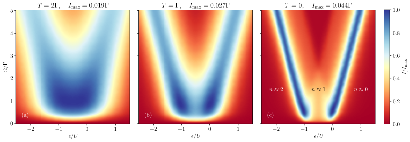
Figure 1: Leading order renormalized perturbation theory at $T=2\Gamma$, $\Gamma$ and $0$: Stationary current as function of interdot hybridization $\Omega$ and dot energies $\epsilon$ for a double quantum dot with interaction $U=5\Gamma$ at bias voltage $V=\Gamma/2$.

We illustrate the dependence of the stationary current on the hybridization $\Omega$ and dot energies $\epsilon$ by sweeping these parameters for three different temperatures $T\in\{0,1,2\}\Gamma$ in Fig. 1 and plot the ratio $I/I_{\text{max}}$, where $I_{\text{max}}$ denotes the maximum current within the scanned parameter range. As expected one can clearly see that the broadening of the transport resonances is decreasing with temperature, but unlike in bare perturbation theory, the width remains finite for $T\rightarrow 0$. Furthermore, as $\Omega\rightarrow 0$ the current vanishes because no tunneling between the dots is possible. This basic feature is completely missed by the popular Pauli master equation, which is even at high temperatures unable to describe the current correctly for $\Omega\lesssim\Gamma$ due to the role of coherences. Other commonly used first order approaches, such as the von Neumann or Redfield approach, which do account for coherences break down when $T\lesssim\Gamma$, see Ref. [Kiršanskas et al., 2017] for a detailed discussion. The two blue lines of maximum current of width $V$ in Fig. 1(c) are due to single electron tunneling (SET) and mark the transition of the stationary total dot occupation $n=n_{1}+n_{2}$ between $2\leftrightarrow 1$ and $1\leftrightarrow 0$ as indicated. We note that cotunneling effects are important away from the resonances and not included consistently through the leading order renormalized perturbation theory. Here the next-to-leading order renormalized perturbation theory or the self-consistent RG methods should be utilized, which are illustrated in the next section.

IV.2 Transient Coulomb diamonds – second order renormalized perturbation theory

We now consider the single impurity Anderson model with energy $\epsilon$, magnetic field $B$ and Coulomb repulsion $U$ described by the Hamiltonian

$$H=\epsilon\left(n_{\uparrow}+n_{\downarrow}\right)+\tfrac{1}{2}B\left(n_{\uparrow}-n_{\downarrow}\right)+Un_{\uparrow}n_{\downarrow}.$$ (38)

The indices $l$ and $\nu$ of Sec. II.1 are spin indices $\sigma$. We take the tunnel rate $\Gamma$ to be spin- and reservoir-independent, i.e., $\Gamma_{r\sigma\sigma^{\prime}}\equiv\Gamma\delta_{\sigma\sigma^{\prime}}$ [Eq. (10)]. The computation of transient occupations using the next-to-leading order renormalized perturbation theory is shown in Listing 3 and the complete code can also be found in the examples folder of the repository. CODE(0x6545b244c318)er the model is set up similarly to before (line 1–8) we use an additional block argument in the computation of the memory kernel and propagator (line 18 and 20). This uses the fact that the memory kernel and propagator are block diagonal, since the particle number and spin component along the magnetic field are conserved. For the considered model the stationary state is encoded in a single block, which can also be used to compute transients as long as the initial state is described by a diagonal density matrix. Thus, only computing a single block accelerates the computation. Omitting the block argument as in Listing 1 defaults to computing the full memory kernel and propagator.

⬇

1// Create Anderson dot with two reservoirs

2Real epsilon = -4; // Dot energy

3Real B = -1; // Magnetic field

4Real U = 10; // Coulomb repulsion

5RealVector T{{0, 0}}; // Temperatures leads

6RealVector mu{{2, -2}}; // Chem. potentials

7RealVector Gamma{{1, 1}}; // Tunnel rate to leads

8auto model = createModel<AndersonDot>(

9 epsilon, B, U, T, mu, Gamma);

10

11// Computation parameters

12Real tMax = 5; // Maximum simulation time

13Real errGoal = 1e-4; // Interpolation error goal

14int block = 0; // Only compute first block

15

16// Compute memory kernel & propagator

17auto method = RenormalizedPT::Order::_2;

18auto K = computeMemoryKernel(

19 model, method, tMax, errGoal, block);

20auto Pi = computePropagator(K, block);

21

22// Set initial state: Basis 0, Up, Down, UpDown

23Matrix rho0 = Matrix::Zero(4, 4);

24rho0.diagonal() << 0, 1, 0, 0;

25

26// Operator nUp

27Matrix nUp = Matrix::Zero(4, 4);

28nUp.diagonal() << 0, 1, 0, 1;

29

30// Compute occupations Tr{nUp*rho(t)}

31auto t = RealVector::LinSpaced(100, 0, tMax);

32RealVector n(t.size());

33for (int i = 0; i < t.size(); ++i)

34 n[i] = (Pi(t[i], rho0) * nUp).trace().real();

35

36// Print

37std::cout << "t = " << t.transpose() << "\n"

38 << "n = " << n.transpose() << "\n";

Listing 3: Computation of transient occupations $\langle n_{\uparrow}\rangle(t)$.

The computation of transient currents is shown in Listing 4. The current kernel is computed (line 10) and used together with the previously obtained propagator in the function computeCurrent (line 14), which returns an object containing a Chebyshev interpolation of the transient current. This allows to efficiently evaluate the current at arbitrary (vectors of) time arguments (line 15).

⬇

8// Compute current kernel

9int r = 0; // Left reservoir

10auto K_I = computeCurrentKernel(

11 model, r, method, tMax, errGoal, block);

12

13// Compute transient current and print

14auto I = computeCurrent(K_I, Pi, rho0);

15RealVector I_t = I(t);

16std::cout << "I = " << I_t.transpose() << "\n";

Listing 4: Computation of the transient currents.

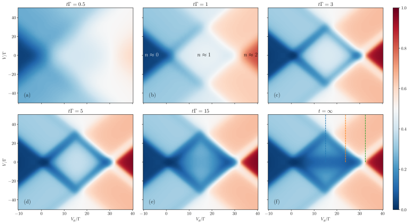
Figure 2: Next-to-leading order renormalized perturbation theory at $T=0$: Transient occupation of the excited state $\langle n_{\uparrow}\rangle(t)$ as function of bias voltage $V=2\mu_{L}=-2\mu_{R}$ and gate voltage $V_{g}=-\epsilon$ for an initially empty Anderson quantum dot $\rho_{0}=|0\rangle\!\langle 0|$ with strong interaction $U=30\Gamma$ and magnetic field $B=5\Gamma$ .

In Fig. 2 we show the transient occupation $\langle n_{\uparrow}\rangle(t)$ for an initially empty dot, $\rho_{0}=|0\rangle\!\langle 0|$, as function of the bias voltage $V$ and gate voltage $V_{g}=-\epsilon$ for several times $t$. These results can be rationalized in detail based on well-established understanding of the stationary limit based on the transition rates. CODE(0x6545b244c318) Fig. 2(a)–(b) fast SET processes fill the dot on a time scale $t\Gamma\sim 1$ to a total number of $n\coloneqq n_{\uparrow}+n_{\downarrow}\approx 1$ and $2$ electrons as indicated in (b) (except in the $n\approx 0$ region where the dot is already stationary). In these regions, the rate of filling is essentially independent of the spin value, allowing the excited level $|\!\!\uparrow\rangle$ to be rapidly occupied with the same probability as the ground level $|\!\!\downarrow\rangle$. In the $n\approx 1$ Coulomb diamond [white center in Fig. 2(b)] this value $n_{\uparrow}\approx 1/2$ exceeds the stationary probability [Fig. 2(f)] and multi-stage decay sets in. At first this decay only occurs along a band of width $\propto B$ inside the Coulomb diamond [dark blue in Fig. 2(c)]. Here the excess energy $B$ of the excited state $|\!\!\uparrow\rangle$ enables SET relaxation indirectly via the empty state $|0\rangle$ to the ground state $|\!\!\downarrow\rangle$ at rate $\propto\Gamma$. We point out that this band is known as the cotunneling-assisted SET (CO-SET) regime in stationary transport, since there the excited level can only be populated by inelastic cotunneling, see Refs. [Leijnse and Wegewijs, 2008; Gaudenzi et al., 2017] and references therein. Here, on the other hand, this band is instead populated by fast SET into the empty dot due to our choice of initial state. Indeed, at this point in time ($t\Gamma\sim 1$) cotunneling has had no time yet to make an impact on the time-dependent transport, as its rate scales as $\propto\Gamma^{2}/U$. This impact is seen only in Fig. 2(d)–(e) where the excitation probability has been reduced uniformly throughout the $n\approx 1$ diamond where SET is energetically forbidden. Here $|\!\!\uparrow\rangle\to|\!\!\downarrow\rangle$ relaxation occurs directly by inelastic cotunneling processes involving both reservoirs and releasing the excess energy $B$. In Fig. 2(f) this reduction has continued at low bias $|V|<B$ whereas it stalls at bias $|V|>B$ in the two visible triangles: only in these regimes excitation $|\!\!\downarrow\rangle\to|\!\!\uparrow\rangle$ by inelastic cotunneling is energetically possible while relaxation by CO-SET is forbidden. This cotunneling re-excitation of the dot effectively counteracts the decay and establishes a sizeable stationary value in competition with cotunneling relaxation. CODE(0x6545b244c318)ortantly, RealTimeTransport allows this rationalization to be further quantified by making use of the time-dependent memory-kernel matrix accessible internally. For example, one interesting avenue would be to construct an effective time-dependent rate picture by converting this memory kernel to a time-local generator. CODE(0x6545b244c318)

IV.3 2-loop RG corrections

We now investigate when it is important to complement the renormalized perturbation theory with the self-consistency imposed by the 2-loop renormalization group transformation. We plot in Fig. 3 the (stationary) nonlinear conductance $dI/dV$ predicted by both methods across the lines indicated in Fig. 2(f). The conductance is computed using a central difference $dI/dV\approx(I(V+\delta V/2)-I(V-\delta V/2))/\delta V$ with $\delta V=0.01\Gamma$. Since we have a substantial magnetic field $B$ the Kondo resonance is not strongly developed here, even at the particle hole symmetric point $\epsilon=-U/2$ (blue curve). Consistent with this, the RG corrections are moderate and occur where they are expected: namely inside the Coulomb diamond they suppress (enhance) the conductance below (above) the onset of ICT at $V\approx B=5\Gamma$ (blue curve). This has the effect of sharpening the ICT onset of the conductance relative to the renormalized perturbation theory. Likewise, the SET signature of the same spin-flip resonance is sharpened. This is in line with the general spirit of our approach as outlined in the introduction: We first introduce too much dissipation to subsequently compute corrections which reduce it in a non-trivial way.

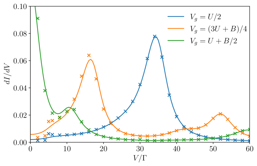
Figure 3: Nonlinear conductance $dI/dV$ at $T=0$ for three gate voltages $V_{g}=-\epsilon$ along the indicated cuts in Fig. 2(f) as predicted by the next-to-leading order renormalized perturbation theory (full lines) and 2-loop renormalization group (crosses) for the same parameters as in Fig. 2.

From a user perspective, performing a calculation with the renormalization group methods is very similar to the perturbation theory methods and is shown in Listing 5. Because the computations are more time consuming it can be useful to parallelize them. We implemented multi-threading capabilities using the Taskflow library. CODE(0x6545b244c318)s allows to define an Executor with a given number of threads (line 3) that can be passed as an additional argument to compute the memory and current kernels (lines 5 and 10).

⬇

1// Set up model and define parameter as before

2// Compute memory kernel with 8 threads

3tf::Executor executor(8);

4auto method = IteratedRG::Order::_2;

5auto K = computeMemoryKernel(model,

6 method, tMax, errGoal, executor);

7auto Pi = computePropagator(K);

8

9// Compute one block of the current kernel

10auto K_I = computeCurrentKernel(K, Pi, r,

11 method, tMax, errGoal, executor, block);

Listing 5: Multi-threaded computation of the memory and current kernel using the RG methods.

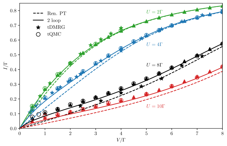
Figure 4: Comparison of the stationary current at $T=0$ as function of the bias $V$ at the symmetry point $\epsilon=-U/2$ and magnetic field $B=0$: next-to-leading order renormalized perturbation theory, 2- and 3-loop RG, tDMRG and the tQMC method.

IV.4 3-loop RG corrections

Finally, we turn to the 3-loop renormalization group corrections at $T=0$. We focus on the particle-hole symmetric point $\epsilon=-U/2$ and the most challenging case of zero magnetic field, $B=0$. In this case the Kondo effect becomes important for small bias $V$, which is challenging to describe for many theoretical methods. CODE(0x6545b244c318)fig:method-comparison-2 we compare the stationary currents obtained from our next-to-leading order renormalized perturbation theory and our 2- and 3-loop renormalization group with the time-dependent density matrix renormalization group (tDMRG) and the real-time quantum Monte Carlo method (tQMC). The data for the latter two were taken from Refs. [Werner, Oka, and Millis, 2009; Heidrich-Meisner, Feiguin, and Dagotto, 2009; Werner et al., 2010], but note also Ref. [Eckel et al., 2010] for further comparisons with the functional renormalization group and the iterative real-time path integral approach. For small interaction $U=2\Gamma$ we find that all methods are largely consistent with each other. The renormalized perturbation theory consistently predicts a current that is too small at low bias $V$, especially for larger interactions shown up to $U=10\Gamma$. This can still be seen in our 2-loop RG, however to a much smaller extent. The 3-loop corrections only become important if $V$ is very small and $U$ is large. Even there we find good overall agreement between the currents predicted by our 3-loop RG and the tQMC method. We note that our discrete RG iteration reproduces the data from the continuous $T$-flow, CODE(0x6545b244c318)firming the expectation that they converge to the same fixed point.

V Summary

We have presented the open source C++ RealTimeTransport library which is available at https://github.com/kn-code/RealTimeTransport to model stationary and transient quantum transport phenomena. The library currently implements four methods: the leading and next-to-leading order renormalized perturbation theory around the infinite temperature limit as well as more advanced 2- and 3-loop renormalization group transformations. We exemplified the practical usage of each of these methods and compared their ranges of applicability. In contrast to the ordinary bare perturbation theory in the tunnel coupling, our renormalized perturbation theory can also be applied all the way down to zero temperature. We have shown that it captures sequential and cotunneling effects in leading and next-to-leading order, respectively. However, especially at low temperatures even higher order effects become important. These can be systematically incorporated using our self-consistent perturbative renormalization group transformation of the memory kernel [Eq. (33)] of increasing loop orders. For an Anderson dot we found that the most advanced 3-loop corrections contribute noticeably only if the system is close to the Kondo resonance. In this case we found overall good agreement between our 3-loop iteration and the tQMC method at finite bias. The version of the library described in this paper is RealTimeTransport 1.0.

Data Availability

The data that support the findings of this study are available from the corresponding author upon reasonable request.

References

References

- Cronenwett, Oosterkamp, and Kouwenhoven (1998) S. M. Cronenwett, T. H. Oosterkamp, and L. P. Kouwenhoven, \csq@thequote@oinit\csq@thequote@oopenA Tunable Kondo Effect in Quantum Dots,\csq@thequote@oclose Science 281, 540–544 (1998).
- Sasaki et al. (2000) S. Sasaki, S. De Franceschi, J. M. Elzerman, W. G. van der Wiel, M. Eto, S. Tarucha, and L. P. Kouwenhoven, \csq@thequote@oinit\csq@thequote@oopenKondo effect in an integer-spin quantum dot,\csq@thequote@oclose Nature 405, 764–767 (2000).
- van der Wiel et al. (2002) W. G. van der Wiel, S. De Franceschi, J. M. Elzerman, T. Fujisawa, S. Tarucha, and L. P. Kouwenhoven, \csq@thequote@oinit\csq@thequote@oopenElectron transport through double quantum dots,\csq@thequote@oclose Rev. Mod. Phys. 75, 1–22 (2002).
- Su et al. (2016) T. A. Su, M. Neupane, M. L. Steigerwald, L. Venkataraman, and C. Nuckolls, \csq@thequote@oinit\csq@thequote@oopenChemical principles of single-molecule electronics,\csq@thequote@oclose Nat. Rev. Mater. 1, 1–15 (2016).
- Gaudenzi et al. (2017) R. Gaudenzi, M. Misiorny, E. Burzurí, M. R. Wegewijs, and H. S. J. van der Zant, \csq@thequote@oinit\csq@thequote@oopenTransport mirages in single-molecule devices,\csq@thequote@oclose J. Chem. Phys. 146 (2017), 10.1063/1.4975767.
- Josefsson et al. (2018) M. Josefsson, A. Svilans, A. M. Burke, E. A. Hoffmann, S. Fahlvik, C. Thelander, M. Leijnse, and H. Linke, \csq@thequote@oinit\csq@thequote@oopenA quantum-dot heat engine operating close to the thermodynamic efficiency limits,\csq@thequote@oclose Nat. Nanotechnol. 13, 920–924 (2018).
- Rammer (2007) J. Rammer, Quantum Field Theory of Non-equilibrium States (Cambridge University Press, Cambridge, England, UK, 2007).
- Metzner et al. (2012) W. Metzner, M. Salmhofer, C. Honerkamp, V. Meden, and K. Schönhammer, \csq@thequote@oinit\csq@thequote@oopenFunctional renormalization group approach to correlated fermion systems,\csq@thequote@oclose Rev. Mod. Phys. 84, 299–352 (2012).
- Schoeller and Schön (1994) H. Schoeller and G. Schön, \csq@thequote@oinit\csq@thequote@oopenMesoscopic quantum transport: Resonant tunneling in the presence of a strong coulomb interaction,\csq@thequote@oclose Phys. Rev. B 50, 18436–18452 (1994).
- Gurvitz and Prager (1996) S. A. Gurvitz and Y. S. Prager, \csq@thequote@oinit\csq@thequote@oopenMicroscopic derivation of rate equations for quantum transport,\csq@thequote@oclose Phys. Rev. B 53, 15932–15943 (1996).
- König, Schoeller, and Schön (1997) J. König, H. Schoeller, and G. Schön, \csq@thequote@oinit\csq@thequote@oopenCotunneling at resonance for the single-electron transistor,\csq@thequote@oclose Phys. Rev. Lett. 78, 4482–4485 (1997).
- Timm (2008) C. Timm, \csq@thequote@oinit\csq@thequote@oopenTunneling through molecules and quantum dots: Master-equation approaches,\csq@thequote@oclose Phys. Rev. B 77, 195416 (2008).
- Koller et al. (2010) S. Koller, M. Grifoni, M. Leijnse, and M. R. Wegewijs, \csq@thequote@oinit\csq@thequote@oopenDensity-operator approaches to transport through interacting quantum dots: Simplifications in fourth-order perturbation theory,\csq@thequote@oclose Phys. Rev. B 82, 235307 (2010).
- Schoeller (2009) H. Schoeller, \csq@thequote@oinit\csq@thequote@oopenA perturbative nonequilibrium renormalization group method for dissipative quantum mechanics,\csq@thequote@oclose Eur. Phys. Journ. Special Topics 168, 179–266 (2009).
- Schoeller (2018) H. Schoeller, \csq@thequote@oinit\csq@thequote@oopenDynamics of open quantum systems,\csq@thequote@oclose (2018), arXiv:1802.10014 [cond-mat.stat-mech] .
- Anders (2008) F. B. Anders, \csq@thequote@oinit\csq@thequote@oopenSteady-state currents through nanodevices: A scattering-states numerical renormalization-group approach to open quantum systems,\csq@thequote@oclose Phys. Rev. Lett. 101, 066804 (2008).
- Nghiem and Costi (2014) H. T. M. Nghiem and T. A. Costi, \csq@thequote@oinit\csq@thequote@oopenGeneralization of the time-dependent numerical renormalization group method to finite temperatures and general pulses,\csq@thequote@oclose Phys. Rev. B 89, 075118 (2014).
- Daley et al. (2004) A. J. Daley, C. Kollath, U. Schollwöck, and G. Vidal, \csq@thequote@oinit\csq@thequote@oopenTime-dependent density-matrix renormalization-group using adaptive effective Hilbertspaces,\csq@thequote@oclose J. Stat. Mech.: Theory Exp. 2004, P04005 (2004).
- White and Feiguin (2004) S. R. White and A. E. Feiguin, \csq@thequote@oinit\csq@thequote@oopenReal-time evolution using the density matrix renormalization group,\csq@thequote@oclose Phys. Rev. Lett. 93, 076401 (2004).
- Schollwöck (2005) U. Schollwöck, \csq@thequote@oinit\csq@thequote@oopenThe density-matrix renormalization group,\csq@thequote@oclose Rev. Mod. Phys. 77, 259–315 (2005).
- Rubtsov, Savkin, and Lichtenstein (2005) A. N. Rubtsov, V. V. Savkin, and A. I. Lichtenstein, \csq@thequote@oinit\csq@thequote@oopenContinuous-time quantum monte carlo method for fermions,\csq@thequote@oclose Phys. Rev. B 72, 035122 (2005).
- Mühlbacher and Rabani (2008) L. Mühlbacher and E. Rabani, \csq@thequote@oinit\csq@thequote@oopenReal-time path integral approach to nonequilibrium many-body quantum systems,\csq@thequote@oclose Phys. Rev. Lett. 100, 176403 (2008).
- Werner, Oka, and Millis (2009) P. Werner, T. Oka, and A. J. Millis, \csq@thequote@oinit\csq@thequote@oopenDiagrammatic monte carlo simulation of nonequilibrium systems,\csq@thequote@oclose Phys. Rev. B 79, 035320 (2009).
- Cohen et al. (2015) G. Cohen, E. Gull, D. R. Reichman, and A. J. Millis, \csq@thequote@oinit\csq@thequote@oopenTaming the dynamical sign problem in real-time evolution of quantum many-body problems,\csq@thequote@oclose Phys. Rev. Lett. 115, 266802 (2015).
- Note (1) The library is available at https://github.com/kn-code/RealTimeTransport.
- Pletyukhov and Schoeller (2012) M. Pletyukhov and H. Schoeller, \csq@thequote@oinit\csq@thequote@oopenNonequilibrium kondo model: Crossover from weak to strong coupling,\csq@thequote@oclose Phys. Rev. Lett. 108, 260601 (2012).
- Bruch et al. (2022) V. Bruch, M. Pletyukhov, H. Schoeller, and D. M. Kennes, \csq@thequote@oinit\csq@thequote@oopenFloquet renormalization group approach to the periodically driven kondo model,\csq@thequote@oclose Phys. Rev. B 106, 115440 (2022).
- Trefethen (2019) L. N. Trefethen, Approximation theory and approximation practice (SIAM, 2019).
- Nestmann and Wegewijs (2022) K. Nestmann and M. R. Wegewijs, \csq@thequote@oinit\csq@thequote@oopenRenormalization group for open quantum systems using environment temperature as flow parameter,\csq@thequote@oclose SciPost Phys. 12, 121 (2022).
- Johansson, Nation, and Nori (2012) J. R. Johansson, P. D. Nation, and F. Nori, \csq@thequote@oinit\csq@thequote@oopenQuTiP: An open-source Python framework for the dynamics of open quantum systems,\csq@thequote@oclose Comput. Phys. Commun. 183, 1760–1772 (2012).
- Johansson, Nation, and Nori (2013) J. R. Johansson, P. D. Nation, and F. Nori, \csq@thequote@oinit\csq@thequote@oopenQuTiP 2: A Python framework for the dynamics of open quantum systems,\csq@thequote@oclose Comput. Phys. Commun. 184, 1234–1240 (2013).
- Kiršanskas et al. (2017) G. Kiršanskas, J. N. Pedersen, O. Karlström, M. Leijnse, and A. Wacker, \csq@thequote@oinit\csq@thequote@oopenQmeq 1.0: An open-source python package for calculations of transport through quantum dot devices,\csq@thequote@oclose Computer Physics Communications 221, 317–342 (2017).
- Bockrath et al. (1997) M. Bockrath, D. H. Cobden, P. L. McEuen, N. G. Chopra, A. Zettl, A. Thess, and R. E. Smalley, \csq@thequote@oinit\csq@thequote@oopenSingle-Electron Transport in Ropes of Carbon Nanotubes,\csq@thequote@oclose Science 275, 1922–1925 (1997).
- Nygård, Cobden, and Lindelof (2000) J. Nygård, D. H. Cobden, and P. E. Lindelof, \csq@thequote@oinit\csq@thequote@oopenKondo physics in carbon nanotubes,\csq@thequote@oclose Nature 408, 342–346 (2000).
- De Franceschi et al. (2001) S. De Franceschi, S. Sasaki, J. M. Elzerman, W. G. van der Wiel, S. Tarucha, and L. P. Kouwenhoven, \csq@thequote@oinit\csq@thequote@oopenElectron cotunneling in a semiconductor quantum dot,\csq@thequote@oclose Phys. Rev. Lett. 86, 878–881 (2001).
- Schleser et al. (2005) R. Schleser, T. Ihn, E. Ruh, K. Ensslin, M. Tews, D. Pfannkuche, D. C. Driscoll, and A. C. Gossard, \csq@thequote@oinit\csq@thequote@oopenCotunneling-mediated transport through excited states in the coulomb-blockade regime,\csq@thequote@oclose Phys. Rev. Lett. 94, 206805 (2005).
- Saptsov and Wegewijs (2014) R. B. Saptsov and M. R. Wegewijs, \csq@thequote@oinit\csq@thequote@oopenTime-dependent quantum transport: Causal superfermions, exact fermion-parity protected decay modes, and pauli exclusion principle for mixed quantum states,\csq@thequote@oclose Phys. Rev. B 90, 045407 (2014).
- Wick, Wightman, and Wigner (1952) G. C. Wick, A. S. Wightman, and E. P. Wigner, \csq@thequote@oinit\csq@thequote@oopenThe intrinsic parity of elementary particles,\csq@thequote@oclose Phys. Rev. 88, 101–105 (1952).
- Aharonov and Susskind (1967) Y. Aharonov and L. Susskind, \csq@thequote@oinit\csq@thequote@oopenCharge superselection rule,\csq@thequote@oclose Phys. Rev. 155, 1428–1431 (1967).
- Nakajima (1958) S. Nakajima, \csq@thequote@oinit\csq@thequote@oopenOn quantum theory of transport phenomena,\csq@thequote@oclose Prog. Theor. Phys. 20, 948 (1958).
- Zwanzig (1960) R. Zwanzig, \csq@thequote@oinit\csq@thequote@oopenEnsemble method in the theory of irreversibility,\csq@thequote@oclose J. Chem. Phys. 33, 1338 (1960).
- Leijnse and Wegewijs (2008) M. Leijnse and M. R. Wegewijs, \csq@thequote@oinit\csq@thequote@oopenKinetic equations for transport through single-molecule transistors,\csq@thequote@oclose Phys. Rev. B 78, 235424 (2008).
- Saptsov and Wegewijs (2012) R. B. Saptsov and M. R. Wegewijs, \csq@thequote@oinit\csq@thequote@oopenFermionic superoperators for zero-temperature nonlinear transport: Real-time perturbation theory and renormalization group for anderson quantum dots,\csq@thequote@oclose Phys. Rev. B 86, 235432 (2012).
- Nestmann and Wegewijs (2021) K. Nestmann and M. R. Wegewijs, \csq@thequote@oinit\csq@thequote@oopenGeneral connection between time-local and time-nonlocal perturbation expansions,\csq@thequote@oclose Phys. Rev. B 104, 155407 (2021).
- Guennebaud, Jacob et al. (2010) G. Guennebaud, B. Jacob, et al., \csq@thequote@oinit\csq@thequote@oopenEigen v3,\csq@thequote@oclose (2010).
- Wegewijs and Nazarov (2001) M. R. Wegewijs and Yu. V. Nazarov, \csq@thequote@oinit\csq@thequote@oopenInelastic co-tunneling through an excited state of a quantum dot,\csq@thequote@oclose arXiv (2001), 10.48550/arXiv.cond-mat/0103579, cond-mat/0103579 .
- Megier, Smirne, and Vacchini (2020) N. Megier, A. Smirne, and B. Vacchini, \csq@thequote@oinit\csq@thequote@oopenThe interplay between local and non-local master equations: exact and approximated dynamics,\csq@thequote@oclose New J. Phys. 22, 083011 (2020).
- Nestmann, Bruch, and Wegewijs (2021) K. Nestmann, V. Bruch, and M. R. Wegewijs, \csq@thequote@oinit\csq@thequote@oopenHow quantum evolution with memory is generated in a time-local way,\csq@thequote@oclose Phys. Rev. X 11, 021041 (2021).
- Huang et al. (2022) T.-W. Huang, D.-L. Lin, C.-X. Lin, and Y. Lin, \csq@thequote@oinit\csq@thequote@oopenTaskflow: A lightweight parallel and heterogeneous task graph computing system,\csq@thequote@oclose IEEE Trans. Parallel Distrib. Syst. 33, 1303–1320 (2022).
- Eckel et al. (2010) J. Eckel, F. Heidrich-Meisner, S. G. Jakobs, M. Thorwart, M. Pletyukhov, and R. Egger, \csq@thequote@oinit\csq@thequote@oopenComparative study of theoretical methods for non-equilibrium quantum transport,\csq@thequote@oclose New Journal of Physics 12, 043042 (2010).
- Heidrich-Meisner, Feiguin, and Dagotto (2009) F. Heidrich-Meisner, A. E. Feiguin, and E. Dagotto, \csq@thequote@oinit\csq@thequote@oopenReal-time simulations of nonequilibrium transport in the single-impurity anderson model,\csq@thequote@oclose Phys. Rev. B 79, 235336 (2009).
- Werner et al. (2010) P. Werner, T. Oka, M. Eckstein, and A. J. Millis, \csq@thequote@oinit\csq@thequote@oopenWeak-coupling quantum monte carlo calculations on the keldysh contour: Theory and application to the current-voltage characteristics of the anderson model,\csq@thequote@oclose Phys. Rev. B 81, 035108 (2010).