Approximating Densest Subgraph in Geometric Intersection Graphs

Abstract

For an undirected graph $\mathsf{G}=(\mathsf{V},\mathsf{E})$, with $n$ vertices and $m$ edges, the densest subgraph problem, is to compute a subset $S\subseteq\mathsf{V}$ which maximizes the ratio ${\left|{\mathsf{E}_{S}}\right|}/{\left|{S}\right|}$, where $\mathsf{E}_{S}\subseteq\mathsf{E}$ is the set of all edges of $\mathsf{G}$ with endpoints in $S$. The densest subgraph problem is a well studied problem in computer science. Existing exact and approximation algorithms for computing the densest subgraph require $\Omega(m)$ time. We present near-linear time (in $n$) approximation algorithms for the densest subgraph problem on implicit geometric intersection graphs, where the vertices are explicitly given but not the edges. As a concrete example, we consider $n$ disks in the plane with arbitrary radii and present two different approximation algorithms.

1 Introduction

Given an undirected graph $\mathsf{G}=(\mathsf{V},\mathsf{E})$, the density of a set $S\subseteq V(\mathsf{G})$ is ${\left|{\mathsf{E}_{S}}\right|}/{\left|{S}\right|}$, where each edge in $\mathsf{E}_{S}\subseteq\mathsf{E}\left({\mathsf{G}}\right)$ has both its vertices in $S$. In the densest subgraph problem, the goal is to find a subset of $V(\mathsf{G})$ with the maximum density. Computing the densest subgraph is a primitive operation in large-scale graph processing, and has found applications in mining closely-knit communities [CS12], link-spam detection [GKT05], and reachability and distance queries [CHKZ03]. See [BKV12] for a detailed discussion on the applications of densest subgraph, and [LMFB23] for a survey on the recent developments on densest subgraph.

Exact algorithms for densest subgraph.

Unlike the (related) problem of computing the largest clique (which is NP-Hard), the densest subgraph can be computed (exactly) in polynomial time. Goldberg [Gol84] show how to reduce the problem to $O(\log n)$ instances of $s{-}t$ min-cut problem. Gallo et al. [GGT89] improved the running time slightly by using parametric max flow computation. Charikar [Cha00] presented an LP based solution to solve the problem, for which Khuller and Saha [KS09] gave a simpler rounding scheme.

Approximation algorithms for densest subgraph.

The exact algorithms described above require solving either an LP or an $s{-}t$ min-cut instance, both of which are relatively expensive to compute. To obtain a faster algorithm, Charikar [Cha00] analyzed a $2$-approximation algorithm which repeatedly removes the vertex with the smallest degree and calculates the density of the remaining graph. This algorithm runs in linear time. After that, Bahmani et al. [BGM14] used the primal-dual framework to give a $(1+\varepsilon)$-approximation algorithm which runs in $O\left({(m/\varepsilon^{2})\log n}\right)$ time. The problem was also studied in the streaming model the focus is on approximation using bounded space. McGregor et al. [MTVV15] and Esfandiari et al. [EHW16] presented a $(1+\varepsilon)$-approximation streaming algorithm using roughly $\widetilde{O}(\left|{\mathsf{V}}\right|)$ space. There has been recent interest in designing dynamic algorithms for approximate densest subgraph, where an edge gets inserted or deleted in each time step [BHNT15, SW20, ELS15].

Geometric intersection graphs.

The geometric intersection graph of a set $\mathcal{D}$ of $n$ objects is a graph $G=(V,E)$, where each object in $\mathcal{D}$ corresponds to a unique vertex in $V$, and an edge exists between two vertices if and only if the corresponding objects intersect. Further, in an implicit geometric intersection graph, the input is only the set of objects $\mathcal{D}$ and not the edge set $\mathsf{E}$, whose size could potentially be quadratic in terms of $\left|{\mathsf{V}}\right|$.

Unlike general graphs, the geometric intersection graphs typically have more structure, and as such computing faster approximation algorithms [AP14, CHQ20], or obtaining better approximation algorithms on implicit geometric intersection graphs has been an active field of research.

One problem closely related to the densest subgraph problem is that of finding the maximum clique. Unlike the densest subgraph problem, the maximum clique problem is NP-hard for various geometric intersection graphs as well (for e.g., segment intersection graphs [CCL13]). However, for the case of unit-disk graphs, an elegant polynomial time solution by Clark et al. [CCJ90] is known.

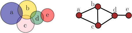
Figure 1.1: Five disks and their corresponding graph. The densest subgraph is $\{a,b,c,d\}$ with density $5/4$.

Motivation.

Densest subgraph computation on geometric intersection graphs can help detect regions which have strong cellular network coverage, or have many polluting factories. The region covered (resp., polluted) by cellular towers (resp., or factories) can be represented by disks of varying radii.

1.1 Problem statement and our results

In this paper we study the densest subgraph problem on implicit geometric intersection graphs, and present near-linear time (in terms of $\left|{\mathsf{V}}\right|$) approximation algorithms.

From reporting to approximate counting/sampling.

We show a reduction from (shallow) range-reporting to approximate counting/sampling. Previous work on closely related problem includes the work by Afshani and Chan [AC09] (that uses shallow counting queries), and the work by Afshani et al. [AHZ10]. The reduction seems to be new, and should be useful for other problems. See Section 3 and Theorem 3.5 for details.

Importantly, this data-structure enables us to sample $(1\pm\varepsilon)$-uniformly a disk from the set of disks intersecting a given disk.

The application.

For the sake of concreteness, we consider the case of $n$ disks (with arbitrary radii) lying in the plane and present two different approximation algorithms. See Figure 1.1.

A $(2+\varepsilon)$-approximation.

Our first approximation algorithm uses the greedy strategy of removing disks of low-degree from the intersection graph. By batching the queries, and using the above data-structure, we get a $(2+\varepsilon)$-approximation for the densest subset of disks in time $O_{\varepsilon}(n\log^{3}n)$, where $O_{\varepsilon}$ hides constants polynomial in $1/\varepsilon$.

A $(1+\varepsilon)$-approximation.

A more promising approach is to randomly sample edges from the intersection graph, and then apply known approximation algorithms. This requires some additional work since unlike previous work, we can only sample approximately in uniform, see Section 5 for details. The running time of the new algorithm is $O_{\varepsilon}(n\log^{2}n\log\log n)$ which is faster than the first inferior $(2+\varepsilon)$-approximation. The results are summarized in Figure 1.2.

Approximation	Running time	Ref
$2+\varepsilon$	$O\bigl{(}\frac{n\log^{2}n}{\varepsilon^{2}}(\tfrac{1}{\varepsilon^{2}}+\log n)\bigr{)}\Bigr{.}$	Theorem 4.3
$1+\varepsilon$	$O\bigl{(}\frac{n\log^{2}n}{\varepsilon^{2}}(\tfrac{1}{\varepsilon^{2}}+\log\log n)\bigr{)}\Bigr{.}$	Theorem 5.9

Figure 1.2: Our results.

2 Preliminaries

2.1 Definitions

In the following, $\mathcal{D}$ denotes a (given) set of $n$ objects (i.e., disks). For $S\subseteq\mathcal{D}$ and $u\in\mathcal{D}$, we use the shorthands $S+u=S\cup\{u\}$ and $S-u=S\setminus\{u\}$. For $\varepsilon\in(0,1)$ and a real number $\alpha>0$, let $(1\pm\varepsilon)\alpha$ denote the interval $\bigl{(}(1-\varepsilon)\alpha,(1+\varepsilon)\alpha\bigr{)}$. Throughout, a statement holds with high probability, if it holds with probability at least $1-n^{-c}$, where $c$ is a sufficiently large constant.

Observation 2.1.

1. For any $\varepsilon$, we have $\frac{1}{1+\varepsilon}\geq 1-\varepsilon$.

2. For $\varepsilon\in(0,1/2)$, we have $\frac{1}{1\pm\varepsilon}=\bigl{(}1/(1+\varepsilon),1/(1-\varepsilon)\bigr{)}\subseteq 1\pm 2\varepsilon$ since $1-\varepsilon\leq\frac{1}{1+\varepsilon}\leq\frac{1}{1-\varepsilon}\leq 1+2\varepsilon.$

3. For $\varepsilon\in(0,1/3)$, we have $(1\pm\varepsilon)^{2}\subseteq(1\pm 3\varepsilon)$.

4. For $\varepsilon\in(0,1)$ and constants $c,c_{1}$ and $c_{2}$, such that $c\geq c_{1}c_{2}$, we have $(1\pm c_{1}\varepsilon/c)(1\pm c_{2}\varepsilon/c)\subseteq 1\pm\frac{c_{1}+c_{2}+1}{c}\varepsilon$.

Definition 2.2.

Given a set of objects $\mathcal{D}$ (say in $\mathbb{R}^{d}$), their intersection graph has an edge between two objects if and only if they intersect. Formally,

$$\mathsf{G}_{\cap\mathcal{D}}=\left({\mathcal{D},\left\{uv\;\middle|\;u,v\in\mathcal{D},\text{ and }u\cap v\neq\emptyset\right\}}\right).$$

Definition 2.3.

For a graph $\mathsf{G}$, and a subset $S\subseteq\mathsf{V}\left({\mathsf{G}}\right)$, let

$$\mathsf{E}_{S}=\mathsf{E}_{S}\left({\mathsf{G}}\right)=\left\{uv\in\mathsf{E}\left({\mathsf{G}}\right)\;\middle|\;u,v\in S\right\}.$$

The induced subgraph of $\mathsf{G}$ over $S$ is $\mathsf{G}_{S}=(S,\mathsf{E}_{S})$, and let $\mathsf{m}\left({S}\right)=\left|{\mathsf{E}_{S}}\right|$ denote the number of edges in this subgraph.

Definition 2.4.

For a set $S\subseteq\mathsf{V}\left({\mathsf{G}}\right)$, its density in $\mathsf{G}$ is ${\nabla}\left({S}\right)=\nabla_{\!\!\mathsf{G}}\left({S}\right)=\mathsf{m}\left({\mathsf{G}_{S}}\right)/\left|{S}\right|,$ where $\mathsf{m}\left({\mathsf{G}_{S}}\right)$ is the number of edges in $\mathsf{G}_{S}$. Similarly, for a set of objects $\mathcal{D}$, and a subset $S\subseteq\mathcal{D}$, the density of $S$ is ${\nabla}\left({S}\right)=\mathsf{m}\left({\mathsf{G}_{\cap S}}\right)/\left|{S}\right|$.

Definition 2.5.

For a graph $\mathsf{G}$, its max density is the quantity $\mathcalb{d}\left({\mathsf{G}}\right)=\max_{S\subseteq\mathsf{V}\left({\mathsf{G}}\right)}{\nabla}\left({S}\right),$ and analogously, for a set of objects $\mathcal{D}$, its max density is $\mathcalb{d}\left({\mathcal{D}}\right)=\max_{S\subseteq\mathcal{D}}{\nabla}\left({S}\right),$

The problem at hand is to compute (or approximate) the maximum density of a set of objects $\mathcal{D}$. If a subset $S$ realizes this quantity, then it is the densest subset of $\mathcal{D}$ (i.e., $\left({\mathsf{G}_{\cap\mathcal{D}}}\right)_{S}$ is the densest subgraph of $\mathsf{G}_{\cap\mathcal{D}}$). One can make the densest subset unique, if there are several candidates, by asking for the lexicographic minimal set realizing the maximum density. For simplicity of exposition we threat the densest subset as being unique.

Lemma 2.6.

Let $\mathcal{O}\subseteq\mathcal{D}$ be the densest subset, and let $\nabla={\nabla}\left({\mathcal{O}}\right)$. Then, for any object $u\in\mathcal{O}$, we have $d_{\mathcal{O}}\left({u}\right)=\left|{u\sqcap(\mathcal{O}-u)}\right|\geq\nabla$, where $u\sqcap(\mathcal{O}-u)=\left\{x\in\mathcal{O}-u\;\middle|\;x\cap u\neq\emptyset\right\}$.

Proof:

Observe that

$$\nabla=\frac{\left|{\mathsf{E}_{\mathcal{O}}}\right|}{\left|{\mathcal{O}}\right|}=\frac{\left|{\mathsf{E}_{\mathcal{O}-u}}\right|+d_{\mathcal{O}}\left({u}\right)}{\left|{\mathcal{O}}\right|-1+1}.$$

As such, if $d_{\mathcal{O}}\left({u}\right)<\nabla$, then

$$\frac{d_{\mathcal{O}}\left({u}\right)}{1}<\nabla=\frac{d_{\mathcal{O}}\left({u}\right)+\left|{\mathsf{E}_{\mathcal{O}-u}}\right|}{1+\left|{\mathcal{O}}\right|-1}<\frac{\left|{\mathsf{E}_{\mathcal{O}-u}}\right|}{\left|{\mathcal{O}}\right|-1}.$$

But this implies that $\mathcal{O}-u$ is denser than $\mathcal{O}$, which is a contradiction.  

2.2 Reporting all intersecting pairs of disks

The algorithm of Section 5 requires an efficient algorithm to report all the intersecting pairs of disks.

Lemma 2.7.

Given a set $\mathcal{D}$ of $n$ disks, all the intersecting pairs of disks of $\mathcal{D}$ can be computed in $O(n\log n+k)$ expected time, where $k$ is the number of intersecting pairs.

Proof:

We break the boundary of each disk at its two $x$-extreme points, resulting in a set of $2n$ $x$-monotone curves. Computing the vertical decomposition of the arrangement of these disks (curves) $\mathcal{A}\left({\mathcal{D}}\right)$ can be done in $O(n\log n+k)$ expected time [Har11]. See Figure 2.1 for an example. This gives us readily all the pairs that their boundaries intersect.

As for the intersections that rise out of containment, perform a traversal of the dual graph of the vertical decomposition (i.e., each vertical trapezoid is a vertex, and two trapezoids are adjacent if they share a boundary edge). The dual graph is planar with $O(n+k)$ vertices and edges, and as such the graph can be traversed in $O(n+k)$ time. During the traversal, by appropriate bookkeeping, it is straightforward to maintain the list of disks containing the current trapezoid, in $O(1)$ per edge traversed, as any edge traversed changes this set by at most one.

For a disk $\mathsf{d}$, let $p_{\mathsf{d}}$ be the rightmost point of $\mathsf{d}$. For each disk $\mathsf{d}$, pick any trapezoid $\Delta$ such that $p_{\mathsf{d}}\in\Delta$ and either the top boundary of $\mathsf{d}$ is the ceiling of $\Delta$ or the bottom boundary of $\mathsf{d}$ is the floor of $\Delta$. Assign $\Delta_{\mathsf{d}}\leftarrow\Delta$ as the representative trapezoid of $\mathsf{d}$.

During the traversal of the dual graph, consider the case where we arrive at a representative trapezoid of a disk $\mathsf{d}$. Let $L(\mathsf{d})$ be the list of disks containing $\Delta_{\mathsf{d}}$. Then scan $L(\mathsf{d})$ to report all the containing pairs of $\mathsf{d}$. Each disk in $L(\mathsf{d})$ either intersects the boundary of $\mathsf{d}$, or contain it. Therefore, the total time spent at the representative trapezoids is $\sum_{\mathsf{d}\in\mathcal{D}}\left|{L(d)}\right|=O(k)$.  

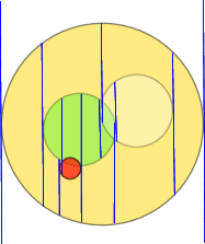
Figure 2.1: Vertical decomposition of four disks.

3 From reporting to approximate sampling/counting

In this section, given a set of objects $\mathcal{D}$, and a reporting data-structure for $\mathcal{D}$, we show a reduction to building a data-structure, such that given a query object $\mathsf{q}$, it returns approximately-at-uniform an object from $\mathsf{q}\sqcap\mathcal{D}=\left\{x\in\mathcal{D}\;\middle|\;x\cap\mathsf{q}\neq\emptyset\right\},$ and also returns an $(1\pm\varepsilon)$-approximation for the size of this set.

3.1 The data-structure

The given reporting data-structure.

Let $\mathcal{D}$ be a set of $n$ objects, and assume for any subset $X\subseteq\mathcal{D}$ of size $m$, one can construct, in $C(m)$ time, a data-structure that given a query object $\mathsf{d}$, returns, in $O(Q(m)+k)$ time, all the objects in $X$ that intersects $\mathsf{d}$, where $k=\left|{\mathsf{d}\sqcap X}\right|$. Furthermore, we assume that if a parameter $k^{\prime}$ is specified by the query, then the data-structure stops after $O(Q(m)+k^{\prime})$ time, if $k>k^{\prime}$, and indicate that this is the case.

Example 3.1.

If $\mathcal{D}$ is a set of disks, and the query $\mathsf{d}$ is a disk, then this becomes a query reporting of the $k$-nearest neighbors in an additive weighted Voronoi diagram. Liu [Liu22] showed how to build such a reporting data-structure, in $O(n\log n)$ expected preprocessing time, and query time $O(\log n+k)$.

Data-structure construction.

We build a random binary tree over the objects of $\mathcal{D}$, by assigning each object of $\mathcal{D}$ with equal probability either a $0$ or a $1$ label. This partitions $\mathcal{D}$ into two sets $\mathcal{D}_{0}$ (label $0$) and $\mathcal{D}_{1}$ (label $1$). Recursively build random trees $T_{0}$ and $T_{1}$ for $\mathcal{D}_{0}$ and $\mathcal{D}_{1}$, respectively, with the output tree having $T_{0}$ and $T_{1}$ as the two children of the root. The constructions bottoms out when the set of objects is of size one. Let $\mathcal{T}$ be the resulting tree that has exactly $n$ leaves. For every node $u$ of $\mathcal{T}$, we construct the reporting data-structure for the set of objects $\mathcal{D}(u)$ – that is, the set of objects stored in the subtree of $u$.

Finally, create an array $L_{i}$ for each level $i$ of the tree $\mathcal{T}$, containing pointers to all the nodes in this level of the tree.

Answering a query.

Given a query object $\mathsf{q}$, and a parameter $\varepsilon\in(0,1/2)$, the algorithm starts from an arbitrary leaf $v$ of $\mathcal{T}$. The leaf $v$ has a unique root to $v$ path, denoted by $\pi=u_{0}u_{1}\ldots u_{t}$, where $u_{0}=\mathrm{root}(\mathcal{T})$ and $u_{t}=v$. The algorithm performs a binary search on $\pi$, using the reporting data-structure associated with each node, to find the maximal $i$, such that $\left|{\mathsf{q}\sqcap\mathcal{D}(u_{i})}\right|>\psi=c\log n$, where $c$ is a sufficiently large constant. Here, we use the property that one can abort the reporting query if the number of reported objects exceeds $\psi$. This implies that each query takes $Q(n)+O(\log n)$ time (with no dependency on $\varepsilon$). Next, the algorithm computes the maximal $j$ such that $\left|{\mathsf{q}\sqcap\mathcal{D}(u_{j})}\right|>\psi_{\varepsilon}=c\varepsilon^{-2}\log n$ (or set $j=0$ if such a $j$ does not exist). This is done by going up the path $\pi$ from $u_{i}$, trying $u_{i-1},u_{i-2},\ldots,u_{j}$ using the reporting data-structure till the condition is fulfilled. Next, the algorithm chooses a vertex $u\in L_{j}$ uniformly at random. It computes the set $S=\mathsf{q}\sqcap\mathcal{D}(u)$ using the reporting data-structure. The algorithm then returns a random object from $S$ uniformly at random, and the number $2^{j}\left|{S}\right|$. The first is a random element chosen from $\mathsf{q}\sqcap\mathcal{D}$, and the second quantity returned is an estimate for $\left|{\mathsf{q}\sqcap\mathcal{D}}\right|$.

3.2 Analysis

3.2.1 Correctness

Lemma 3.2.

Let $\varepsilon\in(0,1/2)$, $\psi_{\varepsilon}=c\varepsilon^{-2}\log n$, and $\mathsf{q}$ be a query object. Let $M\geq 1$ be the integer such that $\psi_{\varepsilon}/16\leq\left|{\mathcal{D}\sqcap\mathsf{q}}\right|/2^{M}<\psi_{\varepsilon}/8.$ Then, for all nodes $v$ at distance $i\leq M$ from the root of $\mathcal{T}$, we have ${\mathbb{P}}\left[\Bigl{.}\smash{\left|{\mathcal{D}(v)\sqcap\mathsf{q}}\right|\notin(1\pm\varepsilon/2)\frac{\left|{\mathcal{D}\sqcap\mathsf{q}}\right|}{2^{i}}}\right]\leq\frac{1}{n^{\Omega(c)}}.$

Proof:

Consider a node $v$ at a distance $i$ from the root, and let $Y_{v}=\left|{\mathcal{D}(v)\sqcap\mathsf{q}}\right|$. Clearly, $\mu_{v}={\mathbb{E}}\left[Y_{v}\right]=\left|{\mathcal{D}\sqcap\mathsf{q}}\right|/2^{i}$. Since $i\leq M$, we have $\mu_{v}\geq\psi_{\varepsilon}/16$. By Chernoff’s inequality, we have

$${\mathbb{P}}\left[\bigl{.}Y_{v}\notin(1\pm\varepsilon/2)\mu_{v}\right]\leq 2\exp\left({-\varepsilon^{2}\mu_{v}/3}\right)\leq 2\exp\left({-\varepsilon^{2}\psi_{\varepsilon}/48}\right)\leq 2\exp\left({-(c/48)\log n}\right)\leq\frac{2}{n^{c/48}}.$$

The number of nodes in $\mathcal{T}$ is $O(n)$, and hence, by the union bound, for all nodes $v$ at distance $i\leq M$ from the root, we have ${\mathbb{P}}\left[Y_{v}\notin(1\pm\varepsilon/2)\mu_{v}\right]\leq{1}/{n^{\Omega(c)}}$.  

Observation 3.3.

Lemma 3.2 implies that for all nodes $v$ at distance $i>M$ from the root of $\mathcal{T}$, we have ${\mathbb{P}}\left[\bigl{.}\left|{\mathcal{D}(v)\sqcap\mathsf{q}}\right|>\psi_{\varepsilon}\right]\leq{1}/{n^{\Omega(c)}}.$ Indeed, Lemma 3.2 implies this for all nodes at distance $M$ from the root, and the sizes of these sets are monotonically decreasing along any path down the tree.

Lemma 3.4.

Assume that the number of distinct sets $\mathsf{q}^{\prime}\sqcap\mathcal{D}$, over all possible query objects $\mathsf{q}^{\prime}$, is bounded by a polynomial $O(n^{d})$, where $d$ is some constant. Then, for a query $\mathsf{q}$, the probability that the algorithm returns a specific object $\mathsf{o}\in\mathcal{D}\sqcap\mathsf{q}$, is in $(1\pm\varepsilon)/\beta$, where $\beta=\left|{\mathcal{D}\sqcap\mathsf{q}}\right|$. Similarly, the estimate the algorithm outputs for $\beta$ is in $(1\pm\varepsilon)\beta$. The answer is correct for all queries, with probability $\geq 1-1/n^{\Omega(c)}$, for a sufficiently large constant $c$.

Proof:

It is easy to verify the algorithm works correctly if $\left|{\mathsf{q}\sqcap\mathcal{D}(u_{j})}\right|<\psi_{\varepsilon}$. Otherwise, for the node $u_{j}$ computed by the algorithm, we have $\left|{\mathsf{q}\sqcap\mathcal{D}(u_{j})}\right|>\psi_{\varepsilon}=c\varepsilon^{-2}\log n$. By Observation 3.3, with high probability, we have that $j\leq M$. By Lemma 3.2, it implies that for any node $u\in L_{j}$, we have $2^{j}\left|{\mathcal{D}(u)\sqcap\mathsf{q}}\right|\in(1\pm\varepsilon/2)\left|{\mathcal{D}\sqcap\mathsf{q}}\right|=(1\pm\varepsilon/2)\beta$, which implies that the estimate for the size of $\beta$ is correct, as $u\in L_{j}$. This readily implies that the probability of returning a specific object $\mathsf{o}\in\mathcal{D}\sqcap\mathsf{q}$ is in $(1\pm\varepsilon)/\beta$, since

$$\frac{1-\varepsilon}{\beta}\leq\frac{1}{(1+\varepsilon/2)\left|{\mathcal{D}\sqcap\mathsf{q}}\right|}\leq\frac{1}{\left|{L_{j}}\right|\cdot\left|{\mathcal{D}(u)\sqcap\mathsf{q}}\right|}\leq\frac{1}{(1-\varepsilon/2)\left|{\mathcal{D}\sqcap\mathsf{q}}\right|}\leq\frac{1+\varepsilon}{\beta}.$$

As for the probabilities, there are $n$ nodes in $\mathcal{T}$, and $O(n^{d})$ different queries, and thus the probability of failure is at most $n^{d+1}/n^{\Omega(c)}<1/n^{\Omega(c)}$, by Lemma 3.2.  

3.2.2 Running times

Query time.

The depth of $\mathcal{T}$ is $h=O(\log n)$ with high probability (follows readily from Chernoff’s inequality). Thus, the first stage (of computing the maximal $i$) requires $O(\log\log n)$ queries on the reporting data-structure, where each query takes $O(Q(n)+\log n)$ time. The second stage (of finding maximal $j$) takes

$$\tau={\mathbb{E}}\left[\Bigl{.}\smash{\sum\nolimits_{t=j}^{i}}O(Q(n)+\left|{\mathcal{D}(u_{t})\sqcap\mathsf{q}}\right|)\right].$$

Thus, we have

1. If $Q(n)=O(\log n)$, then $\tau=O(\psi_{\varepsilon})$, as the cardinality of $\mathcal{D}(u_{t})\sqcap\mathsf{q}$ decreases by a factor of two (in expectation) as one move downward along a path in the tree. Thus $\tau$ is a geometric summation in this case dominated by the largest term.

2. If $Q(n)=\Omega(\log n)$, we have (in expectation) that $\left|{i-j}\right|\leq O(\log(1/\varepsilon))$, and thus $\tau=O(Q(n)\log(1/\varepsilon)+\psi_{\varepsilon})$ time.

3. If $Q(n)=O(n^{\lambda})$, for $0<\lambda\leq 1$, then the query time is dominated by the query time for the top node (i.e., $u_{j}$) in this path, and $\tau=O(Q(n))$, as can easily be verified.

Construction time.

The running time bounds of the form $O(C(n))$ are well-behaved, if for any non-negative integers $n_{1},n_{2},\ldots$, such that $\sum_{i=1}n_{i}=n$, implies that $\sum_{i=1}C(n_{i})=O(C(n))$. Under this assumption on the construction time, we have that the total construction time is $O(C(n)\log n)$.

3.2.3 Summary

Theorem 3.5.

Let $\mathcal{D}$ be a set of $n$ objects, and assume we are given a well-behaved range-reporting data-structure that can be constructed in $C(m)$ time, for $m$ objects, and answers a reporting query $\mathsf{q}$ in $O(Q(m)+\left|{\mathsf{q}\sqcap\mathcal{D}}\right|)$ time. Then, one can construct a data-structure, in $O(C(n)\log n)$ time, such that given a query object $\mathsf{q}$, it reports an $(1\pm\varepsilon)$-estimate for $\beta=\left|{\mathsf{q}\sqcap\mathcal{D}}\right|$, and also returns an object from $\mathsf{q}\sqcap\mathcal{D}$, where each object is reported with probability $(1\pm\varepsilon)/\beta$. The data-structure answers all such queries correctly with probability $\geq 1-1/n^{\Omega(1)}$. The expected query time is:

1. $O((\varepsilon^{-2}+\log\log n)\log n)$ if $Q(m)=O(\log m)$.

2. $O(Q(n))$ if $Q(m)=O(m^{\lambda})$, for some constant $\lambda>0$.

3. $O\bigl{(}\varepsilon^{-2}\log n+Q(n)\log\tfrac{\log n}{\varepsilon})$ otherwise.

Plugging in the data-structure of Liu [Liu22] for disks, with $C(m)=O(m\log m)$, and $Q(m)=O(\log m)$, in the above theorem, implies the following.

Corollary 3.6.

Let $\mathcal{D}$ be a set of $n$ disks in the plane. One can construct in $O(n\log^{2}n)$ time a data-structure, such that given a query disk $\mathsf{q}$ and a parameter $\varepsilon\in(0,1/2)$, it outputs an $(1\pm\varepsilon)$-estimate for $\beta=\left|{\mathsf{q}\sqcap\mathcal{D}}\right|$, and also returns a disk in $\mathsf{q}\sqcap\mathcal{D}$ with a probability that is $(1\pm\varepsilon)$-uniform. The expected query time is $O((\varepsilon^{-2}+\log\log n)\log n)$, and the result returned is correct with high probability for all possible queries.

4 A $(2+\varepsilon)$-approximation for densest subset disks

In this section we design a $(2+\varepsilon)$-approximation algorithm to compute the densest subset of disks in $O(n\varepsilon^{-2}\log^{3}n+n\varepsilon^{-4}\log^{2}n)$ time.

4.1 The algorithm

The input is a set $\mathcal{D}$ of $n$ disks in the plane. Let $\vartheta=\varepsilon/15$. The basic idea is to try a sequence of exponentially decaying values to the optimal density $\mathcalb{d}$. To this end, in the $i$th round, the algorithm would try the degree threshold $\beta=n(1-\vartheta)^{i}$.

In the beginning of such a round, let $\mathcal{L}\leftarrow\mathcal{D}$. During a round, the algorithm repeatedly removes “low-degree” objects, by repeatedly doing the following:

1. The algorithm constructs the data-structure of Corollary 3.6 on the objects of $\mathcal{L}$.

2. Let $\mathcal{L}_{<}\subseteq\mathcal{L}$ be the objects whose degree in $\mathcal{L}$ is smaller than $(1+\vartheta)\beta$ according to this data-structure. Let $\mathcal{L}_{\geq}=\mathcal{L}\setminus\mathcal{L}_{<}$.

3. If $\mathcal{L}_{\geq}$ is empty, then this round failed, and the algorithm continues to the next round.

4. If $\left|{L_{<}}\right|<\vartheta\left|{\mathcal{L}}\right|$, then the algorithm returns $\mathcal{L}$ as the desired approximate densest subset.

5. Otherwise, let $\mathcal{L}\leftarrow\mathcal{L}\setminus L_{<}$. The algorithm continues to the next iteration (still inside the same round).

4.2 Analysis

Lemma 4.1.

When the algorithm terminates, we have $\beta\geq(1-\vartheta)^{3}\mathcalb{d}$, with high probability, where $\mathcalb{d}$ is the optimal density.

Proof:

Consider the iteration when $\beta\in[(1-\vartheta)^{3}\mathcalb{d},(1-\vartheta)^{2}\mathcalb{d}]$. By definition of $\mathcal{L}_{<}$, all the objects in it have a degree at most $(1+\vartheta)\beta\leq(1+\vartheta)(1-\vartheta)^{2}\mathcalb{d}\leq(1-\vartheta)\mathcalb{d}$. By Lemma 2.6, all the objects in the optimal solution have degree $\geq\mathcalb{d}$ (when restricted to the optimal solution). Therefore, none of the objects in the optimal solution are in $\mathcal{L}_{<}$ and hence, the set $\mathcal{L}_{\geq}$ is not empty (and contains the optimal solution). Inside this round, the loop is performed at most $O(\vartheta^{-1}\log n)$ times, as every iteration of the loop shrinks $\mathcal{L}$ by a factor of $1-\vartheta$. This implies that the algorithm must stop in this round.  

Lemma 4.2.

The above algorithm returns a $(2+\varepsilon)$-approximation of the densest subset.

Proof:

Consider the set $\mathcal{L}$, the value of $\beta$ when the algorithm terminated, and let $\nu=\left|{\mathcal{L}}\right|$. By Lemma 4.1, $\beta\geq(1-\vartheta)^{3}\mathcalb{d}$, and by the algorithm stopping condition, we have $\left|{\mathcal{L}_{<}}\right|<\vartheta\left|{\mathcal{L}}\right|.$ In addition, all the objects in $\mathcal{L}_{\geq}$ have degree at least $(1-\vartheta)\beta$. Thus, the number of induced edges on $\mathcal{L}$ is

$$\mathsf{m}\left({\mathcal{L}}\right)\geq\frac{(1-\vartheta)\beta\left|{\mathcal{L}_{\geq}}\right|}{2}>\frac{(1-\vartheta)^{2}\beta\left|{\mathcal{L}}\right|}{2}\geq(1-\vartheta)^{5}\frac{\mathcalb{d}}{2}\left|{\mathcal{L}}\right|\geq(1-5\vartheta)\frac{\mathcalb{d}}{2}\left|{\mathcal{L}}\right|.$$

Thus ${\nabla}\left({\mathcal{L}}\right)=\frac{\mathsf{m}\left({\mathcal{L}}\right)}{\left|{\mathcal{L}}\right|}\geq(1-5\vartheta)\mathcalb{d}/2=(1-\varepsilon/3)\mathcalb{d}/2$, as $\vartheta=\varepsilon/15$. Observe that $2/(1-\varepsilon/3)\leq 2(1+\varepsilon/2)\leq 2+\varepsilon$.  

Theorem 4.3.

Let $\mathcal{D}$ be a set of $n$ disks in the plane, and let $\varepsilon\in(0,1)$ be a parameter. The above algorithm computes, in $O(n\varepsilon^{-2}\log^{3}n+n\varepsilon^{-4}\log^{2}n)$ expected time, a $(2+\varepsilon)$-approximation to the densest subgraph of $\mathsf{G}_{\cap\mathcal{D}}$. The result returned is correct, as is the running time bound, with high probability.

Proof:

The expected time taken in Step-I is $O(n\log^{2}n)$ and the expected time taken in Step-II is $O(n(\vartheta^{-2}+\log\log n)\log n)$. As such, the time taken perform the partition step on $n$ disks is $O(n\log^{2}n+n\vartheta^{-2}\log n)$ expected time.

For a fixed value of $\beta$, let $t$ be the number of times the partition step (i.e., step (V)) is performed, and let $n_{1},n_{2},\ldots,n_{t}$ be the number of objects participating in the partition step. Clearly, $n_{1}=n$, and in general $n_{i}\leq(1-\vartheta)n_{i-1},\forall i\in[2,t]$. Therefore, $\sum_{i=1}^{t}n_{i}=O(n/\vartheta)$ and hence, the expected time taken to perform the $t$ partition steps is $\sum_{i=1}^{t}O(n_{i}\log^{2}n_{i}+n_{i}\vartheta^{-2}\log n_{i})=O(n\vartheta^{-1}\log^{2}n+n\vartheta^{-3}\log n)$. The value of $\beta$ can change $O(\vartheta^{-1}\log n)$ times during the algorithm and hence, the overall expected running time of the algorithm is $O(n\vartheta^{-2}\log^{3}n+n\vartheta^{-4}\log^{2}n)$.  

5 An $(1+\varepsilon)$-approximation for densest subset disks

Here, we present a $(1+\varepsilon)$-approximation algorithm for the densest subset of disks, which is based on the following intuitive idea – if the intersection graph is sparse, then the problem is readily solvable. If not, then one can sample a sparse subgraph, and use an approximation algorithm on the sampled graph.

5.1 Densest subgraph estimation via sampling

Let $\mathsf{G}=(\mathsf{V},\mathsf{E})$ be a graph with $n$ vertices and $m$ edges, with maximum subgraph density $\mathcalb{d}$. Let $\vartheta\in(0,1/6)$ be a parameter, and assume that $m>c^{\prime}n\vartheta^{-2}\log n$, where $c^{\prime}$ is some sufficiently large constant, which in particular implies that

$$\mathcalb{d}=\mathcalb{d}\left({\mathsf{G}}\right)\geq\frac{m}{n}\geq\frac{c^{\prime}}{\vartheta^{2}}\log n.$$

Assume we have an estimate $\overline{m}\in(1\pm\vartheta)m$ of $m$. For a constant $c$ to be specified shortly, with $c<c^{\prime}$, let

$$\psi=c\frac{n}{\overline{m}}\vartheta^{-2}\log n\leq\frac{c}{c^{\prime}(1-\vartheta)}\leq\frac{6c}{5c^{\prime}}<1.$$

Let $F=\{e_{1},\ldots,e_{r}\}$ be a random sample of $r=\left\lceil{\psi\overline{m}}\right\rceil$ edges from $\mathsf{G}$. Specifically, in the $i$th iteration, an edge $e_{i}$ is picked from the graph, where the probability of picking any edge is in $(1\pm\vartheta)/m$. Let $H=(V,F)$, and observe that $H$ is a sparse graph with $n$ vertices and $r=O(\vartheta^{-2}n\log n)$ edges. The claim is that the densest subset $D\subseteq V$ in $H$, or even approximate densest subset, is close to being the densest subset in $\mathsf{G}$. The proof of this follows from previous work [MTVV15], but requires some modifications, since we only have an estimate to the number of edges $m$, and we are also interested in approximating the densest subgraph on the resulting graph. We include the details here so that the presentation is self contained. The result we get is summarized in Lemma 5.4, if the reader is uninterested in the (somewhat tedious) analysis of this algorithm.

5.1.1 Analysis

Lemma 5.1.

Let $\mathcalb{d}=\mathcalb{d}\left({\mathsf{G}}\right)$, and let $U\subseteq V$, be an arbitrary set of $k$ vertices. If $\nabla_{\!\!\mathsf{G}}\left({U}\right)\leq\mathcalb{d}/60$, then ${\mathbb{P}}\left[\nabla_{\!\!H}\left({U}\right)\geq\psi\mathcalb{d}/5\right]\leq n^{-100k}$.

Proof:

We have $\mathcalb{d}\geq m/n$, where $n=\left|{\mathsf{V}\left({\mathsf{G}}\right)}\right|$ and $m=\left|{\mathsf{E}\left({\mathsf{G}}\right)}\right|$, and thus

$$\psi=c\frac{n}{\overline{m}\vartheta^{2}}\log n\geq c\frac{n}{(1+\vartheta)m\vartheta^{2}}\log n\geq\frac{1}{\mathcalb{d}}\cdot\frac{c}{(1+\vartheta)\vartheta^{2}}\log n$$

Let $X_{i}=1$ if the edge sampled in the $i$th round belongs to $H_{U}$ and zero, otherwise. Let $X=\sum_{i}X_{i}$ be the number of edges in $H_{U}$. Then

$${\mathbb{P}}\left[X_{i}=1\right]\in(1\pm\vartheta)\frac{\left|{\mathsf{E}\left({\mathsf{G}_{U}}\right)}\right|}{m}=(1\pm\vartheta)\frac{k\nabla_{\!\!\mathsf{G}}\left({U}\right)}{m}.$$

By linearity of expectations, and as $\overline{m}\in(1\pm\vartheta)m$, we have

$${\mathbb{E}}\left[X\right]\in(1\pm\vartheta)\psi\overline{m}\frac{k\nabla_{\!\!\mathsf{G}}\left({U}\right)}{m}\subseteq(1\pm\vartheta)^{2}\psi k\nabla_{\!\!\mathsf{G}}\left({U}\right).$$ (5.1)

By assumption $\nabla_{\!\!\mathsf{G}}\left({U}\right)\leq\mathcalb{d}/60$, implying that ${\mathbb{E}}\left[X\right]\leq(1+3\vartheta)\psi k\mathcalb{d}/60\leq\psi k\mathcalb{d}/30$, if $\vartheta\in(0,1/3)$, by Observation 2.1. Observe that $(1+(2e-1)){\mathbb{E}}\left[X\right]\leq\frac{\psi k\mathcalb{d}}{5}.$ By Chernoff’s inequality, Lemma A.1, we have

$${\mathbb{P}}\left[\nabla_{\!\!H}\left({U}\right)\geq\frac{\psi\mathcalb{d}}{5}\right] ={\mathbb{P}}\left[X\geq\frac{\psi k\mathcalb{d}}{5}\right]\leq 2^{-\psi k\mathcalb{d}/5}\leq\frac{1}{n^{100k}},$$

by picking $c$ to be sufficiently large.  

Lemma 5.2.

Let $\mathcalb{d}=\mathcalb{d}\left({\mathsf{G}}\right)$, and let $U\subseteq V$, be an arbitrary set of $k$ vertices. If $\nabla_{\!\!\mathsf{G}}\left({U}\right)\geq\mathcalb{d}/60$, then ${\mathbb{P}}\left[\nabla_{\!\!H}\left({U}\right)\in(1\pm\vartheta)^{3}\psi\nabla_{\!\!\mathsf{G}}\left({U}\right)\right]\geq 1-n^{-100k}$ .

Proof:

Following the argument of Lemma 5.1 and as $\nabla_{\!\!\mathsf{G}}\left({U}\right)\geq\mathcalb{d}/60$, we have that ${\mathbb{E}}\left[X\right]=\Omega(k\cdot\psi\nabla_{\!\!\mathsf{G}}\left({U}\right))=\Omega(k\cdot\psi\mathcalb{d})=\Omega(k\cdot c\vartheta^{-2}\log n)$. Chernoff’s inequality, Theorem A.2, then implies that $X\in(1\pm\vartheta){\mathbb{E}}\left[X\right]$ with probability at least $1-2\exp(-\vartheta^{2}{\mathbb{E}}\left[X\right]/4)\geq 1-1/n^{100k}$, for $n$ sufficiently large. The claim now readily follows from Eq. (5.1).  

Lemma 5.3.

Let $\alpha\in(0,1/6)$ be a parameter. For all sets $U\subseteq V$, such that $\nabla_{\!\!H}\left({U}\right)\geq(1-\alpha)\mathcalb{d}\left({H}\right)$, we have that $\nabla_{\!\!\mathsf{G}}\left({U}\right)\geq(1-6\vartheta)(1-\alpha)\mathcalb{d}$, and this holds with high probability.

Proof:

Let $X$ be the densest subset in $\mathsf{G}$. By Lemma 5.2, we have that

$$\nabla_{\!\!H}\left({X}\right)\in(1\pm\vartheta)^{3}\psi\mathcalb{d}\left({\mathsf{G}}\right)\implies\mathcalb{d}\left({H}\right)\geq(1-\vartheta)^{3}\psi\mathcalb{d}\geq\frac{\psi\mathcalb{d}}{2}.$$

By Lemma 5.1, we have that for all the sets $T\subseteq\mathsf{V}$, with $\nabla_{\!\!\mathsf{G}}\left({T}\right)\leq\mathcalb{d}/60$, we have $\nabla_{\!\!H}\left({T}\right)<\psi\mathcalb{d}/5<\mathcalb{d}\left({H}\right)/2$, and this happens with probability $\sum_{k=2}^{n}\sum_{T\subseteq\mathsf{V}:\left|{T}\right|=k}1/n^{100k}\leq\sum_{k=2}^{n}\binom{n}{k}/n^{100k}\leq 1/n^{99}$.

Thus, all the sets $U\subseteq\mathsf{V}$ under consideration have $\nabla_{\!\!\mathsf{G}}\left({U}\right)>\mathcalb{d}/60$. By Lemma 5.2, for all such sets, with probability $1-n^{-100k}\geq 1-1/n^{99}$, we have $\nabla_{\!\!H}\left({U}\right)\in(1\pm\vartheta)^{3}\psi\nabla_{\!\!\mathsf{G}}\left({U}\right)$, which implies $\nabla_{\!\!\mathsf{G}}\left({U}\right)\in\frac{1}{(1\pm\vartheta)^{3}\psi}\nabla_{\!\!H}\left({U}\right).$ Thus, we have

$$\nabla_{\!\!\mathsf{G}}\left({U}\right)\geq\frac{1}{(1+\vartheta)^{3}\psi}\nabla_{\!\!H}\left({U}\right)\geq\frac{(1-\alpha)\mathcalb{d}\left({H}\right)}{(1+\vartheta)^{3}\psi}\geq\frac{(1-\alpha)(1-\vartheta)^{3}\psi\mathcalb{d}}{(1+\vartheta)^{3}\psi}\geq(1-\alpha)(1-6\vartheta)\mathcalb{d},$$

since $1/(1+\vartheta)\geq 1-\vartheta$, and $(1-\vartheta)^{6}\geq 1-6\vartheta$.  

5.1.2 Summary

Lemma 5.4.

Let $\varepsilon\in(0,1)$ be a parameter, and let $\mathsf{G}=(\mathsf{V},\mathsf{E})$ be a graph with $n$ vertices and $m$ edges, with $m=\Omega(\varepsilon^{-2}n\log n)$. Furthermore, let $\overline{m}$ be an estimate to $m$, such that $\overline{m}\in(1\pm\vartheta)m$, where $\vartheta=\varepsilon/10$. Let $\psi=c(n/\overline{m})\vartheta^{-2}\log n$, and let $F$ be a random sample of $\psi\overline{m}=O(\varepsilon^{-2}n\log n)$ edges, with repetition, where the probability of any specific edge to be picked is $(1\pm\vartheta)/m$, and $c$ is a sufficiently large constant. Let $H=(\mathsf{V},F)$ be the resulting graph, and let $X\subseteq\mathsf{V}$ be subset of $H$ with $\nabla_{\!\!H}\left({X}\right)\geq(1-\varepsilon/6)\mathcalb{d}\left({H}\right)$. Then, ${\nabla}\left({X}\right)\geq(1-\varepsilon)\mathcalb{d}\left({\mathsf{G}}\right)$.

Proof:

This follows readily from the above, by setting $\alpha=\varepsilon/6$, and using Lemma 5.3.  

5.2 Random sampler

To implement the above algorithm, we need an efficient algorithm for sampling edges from the intersection graph of disks, which we describe next.

5.2.1 The algorithm

The algorithm consists of the following steps:

1. Build the data-structure of Corollary 3.6 on the disks of $\mathcal{D}$ with error parameter $\varepsilon/c$, where $c$ is a sufficiently large constant. Also, build the range-reporting data-structure of Liu [Liu22] on the disks of $\mathcal{D}$.

2. For each object $\mathsf{o}\in\mathcal{D}$, query the data-structure of Corollary 3.6 with $\mathsf{o}$. Let the estimate returned be $d^{\prime}$. If $d^{\prime}<c^{\prime}/\varepsilon$ (for a constant $c^{\prime}\gg c$), then report $\mathsf{o}\sqcap\mathcal{D}$ by querying the range-reporting data-structure with $\mathsf{o}$, and set $d_{\mathsf{o}}\leftarrow|\mathsf{o}\sqcap\mathcal{D}|-1$. Otherwise, set $d_{\mathsf{o}}\leftarrow d^{\prime}$.

3. We perform $|F|$ iterations and in each iteration, sample a random edge from $\mathsf{G}_{\cap\mathcal{D}}$. In a given iteration, sample a disk $\mathsf{o}\in\mathcal{D}$, where $\mathsf{o}$ has a probability of $\frac{d_{\mathsf{o}}}{\sum_{\mathsf{o}\in\mathcal{D}}d_{\mathsf{o}}}$ being sampled. If $d_{\mathsf{o}}<c^{\prime}/\varepsilon$, then uniformly-at-random report a disk from $\mathsf{o}\sqcap(\mathcal{D}-\mathsf{o})$. Otherwise, query the data-structure of Corollary 3.6 with $\mathsf{o}$ which returns a disk in $\mathsf{o}\sqcap\mathcal{D}$ (keep querying till a disk other than $\mathsf{o}$ is returned).

5.2.2 Analysis

Lemma 5.5.

For each object $\mathsf{o}\in\mathcal{D}$, we have $d_{\mathsf{o}}\in(1\pm\varepsilon/c^{\prime\prime})|\mathsf{o}\sqcap(\mathcal{D}-\mathsf{o})|$, where $c\gg c^{\prime\prime}$ with high probability.

Proof:

Fix an object $\mathsf{o}$. When $d^{\prime}<c^{\prime}/\varepsilon$, then the statement holds trivially. Let ${d}=|\mathsf{o}\sqcap(\mathcal{D}-\mathsf{o})|$. Now we consider the case $d^{\prime}\geq c^{\prime}/\varepsilon$. We know that $d^{\prime}\in(1\pm\varepsilon/c)({d}+1)$. Firstly, $d^{\prime}\leq(1+\varepsilon/c)({d}+1)\leq(1+\varepsilon/c^{\prime\prime}){d}$ hold if

$${d}\geq\frac{1}{\varepsilon}\cdot\frac{1+\varepsilon/c}{1/c^{\prime\prime}-1/c}\geq 1/2\varepsilon.$$

Observe that ${d}\geq 1/2\varepsilon$, since $c^{\prime}/\varepsilon\leq d^{\prime}\leq(1+\varepsilon/c)({d}+1)$ implies that ${d}\geq\frac{c^{\prime}}{\varepsilon(1+\varepsilon/c)}-1\geq 1/2\varepsilon$. Finally, $d^{\prime}\geq(1-\varepsilon/c)({d}+1)\geq(1-\varepsilon/c^{\prime\prime}){d}$ holds trivially. Therefore,

$$d_{\mathsf{o}}=d^{\prime}\in(1\pm\varepsilon/c^{\prime\prime}){d}.$$

 

Lemma 5.6.

In each iteration, the probability of sampling any edge in $\mathsf{G}_{\cap\mathcal{D}}$ is $(1\pm\varepsilon)/m$.

Proof:

An edge $(u,v)$ in $\mathsf{G}_{\cap\mathcal{D}}$ can get sampled in step (III) in two ways. In the first way, the disk corresponding to $u$ gets sampled and then $v$ gets reported as the random neighbor of $u$, and vice-versa for the second way.

Let $d=|\mathsf{o}\sqcap(\mathcal{D}-\mathsf{o})|$, where $\mathsf{o}$ is the disk corresponding to $u$. Consider the case, where $d_{\mathsf{o}}\geq c^{\prime}/\varepsilon$. As such, the first way of sampling the edge $(u,v)$ has probability lower-bounded by:

$$\frac{d_{\mathsf{o}}}{\sum d_{\mathsf{o}}}\cdot\underbrace{\frac{1\pm\varepsilon/c}{d}}_{\text{almost-uniformity}}\subseteq\frac{d_{\mathsf{o}}}{\underbrace{(1\pm\varepsilon/c^{\prime\prime})2m}_{\hyperref@@ii[lemma:approx-degree]{Lemma~{}\ref*{lemma:approx-degree}}}}\cdot\frac{1\pm\varepsilon/c}{d}\subseteq\frac{(1\pm\varepsilon/c^{\prime\prime})d}{(1\pm\varepsilon/c^{\prime\prime})2m}\cdot\frac{1\pm\varepsilon/c}{d}\subseteq\frac{1\pm\varepsilon}{2m}.$$

Therefore, for the case $d_{\mathsf{o}}\geq c^{\prime}/\varepsilon$, the probability of sampling the edge $(u,v)$ is $(1\pm\varepsilon)/m$. Similarly, the statement holds for the case $d_{\mathsf{o}}<c^{\prime}/\varepsilon$.  

Lemma 5.7.

The expected running time of the algorithm is $O(\varepsilon^{-4}n\log^{2}n+\varepsilon^{-2}n\log^{2}n\cdot\log\log n)$.

Proof:

The first step of the algorithm takes $O(n\log^{2}n)$ expected time. The second step of the algorithm takes $O(n(\varepsilon^{-2}+\log\log n)\log n)$ expected time. In the third step of the algorithm, each iteration requires querying the data-structure of Corollary 3.6 $O(1)$ times in expectation. Therefore, the third step takes $O(|F|)\cdot O((\varepsilon^{-2}+\log\log n)\log n)=O(\varepsilon^{-4}n\log^{2}n+\varepsilon^{-2}n\log^{2}n\cdot\log\log n)$ expected time.   

The above implies the following result.

Lemma 5.8.

Let $\mathcal{D}$ be a collection of $n$ disks in the plane, and let $\mathsf{G}_{\cap\mathcal{D}}$ be the corresponding geometric intersection graph with $m$ edges. Let $F$ be a random sample of $O(\varepsilon^{-2}n\log n)$ edges from $\mathsf{G}_{\cap\mathcal{D}}$, with repetition, where the probability of any specific edge to be picked is $(1\pm\varepsilon)/m$. The edges are all chosen independently into $F$. Then, the algorithm described above, for computing $F$, runs in $O(\varepsilon^{-4}n\log^{2}n+\varepsilon^{-2}n\log^{2}n\cdot\log\log n)$ expected time.

5.3 The result

Theorem 5.9.

Let $\mathcal{D}$ be a collection of $n$ disks in the plane. A $(1+\varepsilon)$-approximation to the densest subgraph of $\mathcal{D}$ can be computed in $O(\varepsilon^{-4}n\log^{2}n+\varepsilon^{-2}n\log^{2}n\cdot\log\log n)$ expected time. The correctness of the algorithm holds with high probability.

Proof:

The case of intersection graph having $O(\varepsilon^{-2}n\log n)$ edges can be handled directly by computing the whole intersection graph in $O(\varepsilon^{-2}n\log n)$ expected time (using Lemma 2.7).

To handle the other case, we use Lemma 5.8 to generate a graph $H=(\mathsf{V},F)$ in $O(\varepsilon^{-4}n\log^{2}n+\varepsilon^{-2}n\log^{2}n\cdot\log\log n)$ expected time. Since the intersection graph has $\Omega(\varepsilon^{-2}n\log n)$ edges, using Lemma 5.4, it suffices to compute a $(1-\varepsilon/6)$ approximate densest subgraph of $H$, which can be computed by the algorithm of [BGM14] in $O(\varepsilon^{-4}n\log^{2}n)$ expected time.  

6 Conclusions

We presented two near-linear time approximation algorithms to compute the densest subgraph on (implicit) geometric intersection graph of disks. We conclude with a few open problems. It seems that the running time of the $(2+\varepsilon)$-approximation algorithm can be improved to $O_{\varepsilon}(n\log n)$: the deepest point in the arrangement of the disks and the densest subgraph are mutually bounded by a constant factor, and a $(1+\vartheta)$-approximation of the deepest point in the arrangement of the disks can be computed in $O(\vartheta^{-2}n\log n)$ time [AH08].

Are there implicit geometric intersection graphs, such as unit-disk graphs or say, interval graphs, for which the exact densest subgraph can be computed in sub-quadratic time (in terms of $n$)? Finally, maintaining the approximate densest subgraph in sub-linear time (again in terms of $n$) under insertions and deletions of objects, looks to be a challenging problem (in prior work on general graphs an edge gets deleted or inserted, but in an intersection graph a vertex gets deleted or inserted).

Appendix A Chernoff’s inequality

The following are standard forms of Chernoff’s inequality, see [MR95].

Lemma A.1.

Let $X_{1},\ldots,X_{n}$ be $n$ independent Bernoulli trials, where ${\mathbb{P}}\left[X_{i}=1\right]=p_{i},$ and ${\mathbb{P}}\left[X_{i}=0\right]=1-p_{i},$ for $i=1,\ldots,n$. Let $X=\sum_{i=1}^{b}X_{i}$, and $\mu={\mathbb{E}}\left[\bigl{.}X\right]=\sum_{i}p_{i}$. For $\delta>2e-1$, we have ${\mathbb{P}}\left[\bigl{.}X>(1+\delta)\mu\right]<2^{-\mu(1+\delta)}$.

Theorem A.2.

Let $\varepsilon\in(0,1)$ be a parameter. Let $X_{1},\ldots,X_{n}\in[0,1]$ be $n$ independent random variables, let $X=\sum_{i=1}^{n}X_{i}$, and let $\mu={\mathbb{E}}\left[X\right]$. We have that

$${\mathbb{P}}\left[\bigl{.}{X}\notin(1\pm\varepsilon)\mu\right]\leq 2\exp\left({-\varepsilon^{2}\mu/3}\right)$$

References

- [AC09] Peyman Afshani and Timothy M. Chan “Optimal halfspace range reporting in three dimensions” In Proc. 20th ACM-SIAM Sympos. Discrete Algs. (SODA) SIAM, 2009, pp. 180–186 DOI: 10.1137/1.9781611973068.21
- [AH08] Boris Aronov and Sariel Har-Peled “On Approximating the Depth and Related Problems” In SIAM Journal of Computing 38.3, 2008, pp. 899–921
- [AHZ10] Peyman Afshani, Chris H. Hamilton and Norbert Zeh “A general approach for cache-oblivious range reporting and approximate range counting” In Comput. Geom. 43.8, 2010, pp. 700–712 DOI: 10.1016/J.COMGEO.2010.04.003
- [AP14] Pankaj K. Agarwal and Jiangwei Pan “Near-Linear Algorithms for Geometric Hitting Sets and Set Covers” In Proceedings of Symposium on Computational Geometry (SoCG), 2014, pp. 271
- [BGM14] Bahman Bahmani, Ashish Goel and Kamesh Munagala “Efficient Primal-Dual Graph Algorithms for MapReduce” In Algorithms and Models for the Web Graph: 11th International Workshop, 2014, pp. 59–78
- [BHNT15] Sayan Bhattacharya, Monika Henzinger, Danupon Nanongkai and Charalampos E. Tsourakakis “Space- and Time-Efficient Algorithm for Maintaining Dense Subgraphs on One-Pass Dynamic Streams” In Proceedings of ACM Symposium on Theory of Computing (STOC), 2015, pp. 173–182
- [BKV12] Bahman Bahmani, Ravi Kumar and Sergei Vassilvitskii “Densest Subgraph in Streaming and MapReduce” In Proceedings of the VLDB Endowment 5.5, 2012, pp. 454–465
- [CCJ90] Brent N. Clark, Charles J. Colbourn and David S. Johnson “Unit disk graphs” In Discrete Mathematics 86.1-3, 1990, pp. 165–177
- [CCL13] Sergio Cabello, Jean Cardinal and Stefan Langerman “The Clique Problem in Ray Intersection Graphs” In Discrete & Computational Geometry 50.3, 2013, pp. 771–783
- [Cha00] Moses Charikar “Greedy approximation algorithms for finding dense components in a graph” In Proceedings of Approximation Algorithms for Combinatorial Optimization Problems (APPROX), 2000, pp. 84–95
- [CHKZ03] Edith Cohen, Eran Halperin, Haim Kaplan and Uri Zwick “Reachability and Distance Queries via 2-Hop Labels” In SIAM Journal of Computing 32.5, 2003, pp. 1338–1355
- [CHQ20] Chandra Chekuri, Sariel Har-Peled and Kent Quanrud “Fast LP-based Approximations for Geometric Packing and Covering Problems” In Proc. 31st ACM-SIAM Sympos. Discrete Algs. (SODA), 2020, pp. 1019–1038
- [CS12] Jie Chen and Yousef Saad “Dense Subgraph Extraction with Application to Community Detection” In IEEE Transactions on Knowledge and Data Engineering (TKDE) 24.7, 2012, pp. 1216–1230
- [EHW16] Hossein Esfandiari, MohammadTaghi Hajiaghayi and David P. Woodruff “Brief Announcement: Applications of Uniform Sampling: Densest Subgraph and Beyond” In Proceedings of Symposium on Parallelism in Algorithms and Architectures (SPAA), 2016, pp. 397–399
- [ELS15] Alessandro Epasto, Silvio Lattanzi and Mauro Sozio “Efficient Densest Subgraph Computation in Evolving Graphs” In Proceedings of International World Wide Web Conferences (WWW), 2015, pp. 300–310
- [GGT89] Giorgio Gallo, Michael D. Grigoriadis and Robert Endre Tarjan “A Fast Parametric Maximum Flow Algorithm and Applications” In SIAM Journal of Computing 18.1, 1989, pp. 30–55
- [GKT05] David Gibson, Ravi Kumar and Andrew Tomkins “Discovering Large Dense Subgraphs in Massive Graphs” In Proceedings of Very Large Data Bases (VLDB), 2005, pp. 721–732
- [Gol84] A.. Goldberg “Finding a Maximum Density Subgraph” Berkeley, CA, USA: University of California at Berkeley, 1984
- [Har11] Sariel Har-Peled “Geometric Approximation Algorithms” 173, Math. Surveys & Monographs Boston, MA, USA: Amer. Math. Soc., 2011 DOI: 10.1090/surv/173
- [KS09] Samir Khuller and Barna Saha “On Finding Dense Subgraphs” In Proceedings of International Colloquium on Automata, Languages and Programming (ICALP), 2009, pp. 597–608
- [Liu22] Chih-Hung Liu “Nearly Optimal Planar $k$ Nearest Neighbors Queries under General Distance Functions” In SIAM J. Comput. 51.3, 2022, pp. 723–765 DOI: 10.1137/20M1388371
- [LMFB23] Tommaso Lanciano, Atsushi Miyauchi, Adriano Fazzone and Francesco Bonchi “A Survey on the Densest Subgraph Problem and its Variants” In CoRR abs/2303.14467, 2023
- [MR95] Rajeev Motwani and Prabhakar Raghavan “Randomized Algorithms” Cambridge, UK: Cambridge University Press, 1995 URL: http://us.cambridge.org/titles/catalogue.asp?isbn=0521474655
- [MTVV15] Andrew McGregor, David Tench, Sofya Vorotnikova and Hoa T. Vu “Densest Subgraph in Dynamic Graph Streams” In Proceedings of Mathematical Foundations of Computer Science (MFCS), 2015, pp. 472–482
- [SW20] Saurabh Sawlani and Junxing Wang “Near-optimal fully dynamic densest subgraph” In Proceedings of ACM Symposium on Theory of Computing (STOC), 2020, pp. 181–193