Abstract

E. coli use a regular lattice of receptors and attached kinases to detect and amplify faint chemical signals. Kinase output is characterized by precise adaptation to a wide range of background ligand levels and large gain in response to small relative changes in ligand concentration. These characteristics are well described by models which achieve their gain through equilibrium cooperativity. But these models are challenged by two experimental results. First, neither adaptation nor large gain are present in receptor binding assays. Second, in cells lacking adaptation machinery, fluctuations can sometimes be enormous, with essentially all kinases transitioning together. Here we introduce a far-from equilibrium model in which receptors gate the spread of activity between neighboring kinases. This model achieves large gain through a mechanism we term lattice ultrasensitivity (LU). In our LU model, kinase and receptor states are separate degrees of freedom, and kinase kinetics are dominated by chemical rates far-from-equilibrium rather than by equilibrium allostery. The model recapitulates the successes of past models, but also matches the challenging experimental findings. Importantly, unlike past lattice critical models, our LU model does not require parameters to be fine tuned for function.

Introduction

The chemotaxis signaling pathway used by E. coli for run and tumble navigation is perhaps the best understood biological circuit. Predictive models can accurately describe the response of CheA kinase activity – the signaling output – to arbitrary time-varying inputs of ligand concentration [1, 2, 3, 4] either in bulk experiments [5, 6] or in individual cells [7, 8, 9, 10, 11]. The most striking features of these measurements are large gain and precise adaptation (Fig. 1A); following a small step change in attractant concentration, CheA activity responds in a fast, highly amplified manner (large gain). Methyltransferase CheR and methylesterase CheB then methylate and demethylate receptors, slowly adapting the system output back to its original, steady-state level (precise adaptation). The proteins that implement these dynamics are well characterized and known structurally at atomic resolution [12, 13, 14]. Strikingly, the ligand receptors, CheA kinases, and an adaptor protein, CheW, are arrayed in a stable Kagome lattice [15, 16, 17], with each core unit containing one CheA homodimer, two CheW, and two trimers of receptor dimers [18, 19]. While these components are mostly fixed in a rigid lattice, the phospho-acceptor domain of CheA, P1, is attached only by a roughly 20nm flexible linker [20, 21, 22, 23].

Despite this wealth of data and phenomenological modeling across scales, the broad principles by which the signaling array achieves its large gain remain unclear. Most past work has understood amplification as arising from either Monod-Wyman-Changeux (MWC) cooperativity, or from two dimensional Ising interactions between receptors in the lattice [24, 25, 26, 27, 28, 1, 2, 3, 29, 9, 11]. In each case, receptors are modeled as equilibrium two-state systems with the active state having lower affinity for ligand than the inactive one, and with methylation shifting the free energy difference between these states. In models with MWC cooperativity, groups of receptors organize into tight clusters which must change states together [1, 9, 3]. In Ising-like models, neighboring receptors have an energetic coupling that causes them to prefer the same state [25, 28, 2, 3]; when this coupling is near a critical value, long-range correlations in the lattice create very large effective clusters of receptors which are likely to change states together. In both classes of models, receptor state locally modulates the activity of associated kinases, which do not have their own independent degrees of freedom. Thus, while the kinase consumes chemical energy in the form of ATP, their regulation is understood as being essentially equilibrium.

While these broad pictures are consistent with most existing data, they are difficult to reconcile with two sets of observations. The first observation was made using radioligand approaches to examine receptor binding in addition to the normally measured kinase activity [30, 31]. These studies found that adaptation and large gain are both almost entirely absent at the receptor level, appearing only at the level of kinase activity (Fig. 1B). This decoupling suggests that a mechanistic model for large gain must include separate degrees of freedom for receptors and kinases. Equilibrium Ising and MWC models have a bidirectional coupling between receptors and kinases, making such separate degrees of freedom problematic. Indeed, recent theoretical work argues that the coupling between receptors and kinases must be out of equilibrium to account for these results [32].

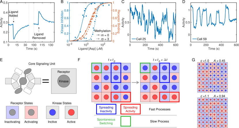
Figure 1: Key experimental results in chemosensing (A-D) and an overview of the lattice ultrasensitivity model (E-G). A) Activity of CheA responds quickly to changes in ligand concentration, then slowly and precisely adapts back to pre-stimulus level via methylation of receptors. Data is from Ref. [33]. B) CheA activity curves shift with mean receptor methylation and show relatively large gain, while receptor binding has lower gain and minimal dependency on methylation. Lines were obtained by fitting data to Hill functions. Data is from Ref. [31]. C) Individual cells can exhibit very large fluctuations, spreading over almost the entire range of possible activities. Data is from Ref. [7]. D) Some cells exhibit almost binary, two-state switching in the absence of adaptation enzymes. Data is from Ref. [7]. E) CheA kinases are represented by circles, whose color indicates their activity state (active or inactive). Receptors are represented by the surrounding squares, and their color indicates a preference for spreading of activity vs inactivity. F) Examples of spreading and spontaneous switching. The two configurations show one realization of each process occurring on a lattice in a time $\Delta t$. Colored rectangular outlines highlight the core units impacted by the processes indicated below. The probability of spreading activity or inactivity depends on the control parameter $c$, defined as the ratio of total rates of kinase activation and deactivation, which themselves depend on receptor occupancy and methylation. In this case $c=1$. G) Representative lattice configurations illustrate how a small change in the control parameter $c$ has a large impact on kinase activity. The changes to receptors and paths of activity spreading (the distribution of square colors) when increasing $c$ from $1$ to $1.1$ is barely noticeable. However, because this change crosses the percolation critical point, the number of active (red) kinases, and thus the average activity $A$, changes dramatically.

The second observation came from measurements of spontaneous fluctuations generated in the chemoreceptor array. First characterized by monitoring the flagellar motor output downstream of kinases [34, 35, 36], advances in FRET microscopy made it possible to more directly measure fluctuations in the kinase activity of individual cells [7, 8]. Assuming fluctuations originate in stochastic switching of MWC clusters, the variance of these fluctuations should be inversely proportional to the number of signaling units. Fluctuations in most non-adapting cells ($\Delta cheRB$) are compatible with this. However, much larger fluctuations are observed in adapting cells and in non-adapting cells exposed to a constant, finely tuned ligand concentration which brings their activities to the middle of their dynamic ranges (Fig. 1C). About 15% of these cells even exhibit “two-state switching” where all kinases in a cell undergo coordinated changes in activity (Fig. 1D). An Ising model can produce these fluctuations if it is tuned very close to its critical point [37, 38], but doing so creates another difficulty: the need for fine tuning. This is true of most models with lattice critical points. Reaching the Ising critical point requires fine-tuning two parameters: the strength of coupling between neighboring units and the bias towards activity or inactivity in single units. While methylation kinetics explain tuning of activity bias, coupling would need to be fine-tuned either through evolution or through another as yet unidentified mechanism.

Here we present a new mechanism for achieving large gain in a lattice critical model that does not require any explicit fine-tuning. In our lattice model, individual receptors bind ligand independently of kinase activity and methylation level, so receptor occupancy and the corresponding dose-response curves exhibit neither gain nor adaptation. This occupancy determines the state of the receptor, which can be kinase-activating or kinase-inactivating. This is a separate degree of freedom from the state of kinase activity (Fig. 1E). Using the chemical energy released by ATP hydrolysis, kinase dynamics are inherently out of equilibrium. Kinase activity and inactivity spread through the lattice in a way that depends non-reciprocally on both receptor state and methylation (Fig. 1F). Specifically, kinase activity spreads with a methylation-dependent rate from an active kinase to an inactive neighbor, but only if the receptor associated with the inactive kinase is in the activating state. Inactivity spreads similarly through the lattice from an inactive to an active kinase through inactivating receptors and with a different methylation-dependent rate. With these rules, large gain is only present at the kinase level and arises due to the singular mapping between the size of connected clusters of kinase activity and the fraction of activating receptors in a percolation-like transition (Fig. 1G).

More quantitatively, the opposing spread of inactivity and activity in our model achieves gain in a way which is mathematically equivalent to the zero-order ultrasensitivity described by Goldbeter and Koshland [39], wherein the concentration of the product of an enzymatic futile cycle depends sharply on the ratio of the rates of the forward and backwards enzyme activities. For this reason, we call our model for signal amplification the lattice ultrasensitivity (LU) model.

Using both an analytic mean field model and stochastic simulations, we will show that the LU model agrees with measurements of both enormous fluctuations [7, 8] and non-adapting, non-cooperative ligand binding [30, 31], while retaining the excellent agreement to other experimental results. Functionally, our model suggests a mechanism by which bacteria could achieve large gain using an energy consuming lattice critical point without the need for explicitly fine-tuned parameters.

Model and Results

We begin with an overview of the LU model without adaptation, and analyze how it achieves large gain, introducing a mean field approximation. We then discuss incorporating adaptation, and show how the LU model reproduces key features of observed noise spectra.

Lattice ultrasensitivity model distinguishes between receptor and kinase states

Motivated by the observation that kinase activity exhibits adaptation and large gain while receptor binding does not, we model kinases and receptors as distinct units. Inspired by their arrangement in a large regular lattice [15], kinases and receptors occupy the vertices of a simplified square lattice in our simulations (Fig. 1E,F). Receptors have two states, kinase-activating and -inactivating, that bind ligand with different affinities. Separately, receptors also have a methylation level, $m$, which takes values between 0 and 4, corresponding to the fully demethylated and methylated states, respectively. We assume that receptor state and ligand binding dynamics (but not methylation) are in equilibrium and fast relative to other timescales in the model. The probability $p$ that a receptor is activating is then given by the instantaneous ligand concentration $[L]$ via

$$p([L])=(1+e^{\Delta f([L])})^{-1},$$ (1)

where $\Delta f([L])$ denotes the ligand-dependent free energy difference between activating and inactivating receptors:

$$\Delta f([L])=\Delta f_{0}+\mathrm{log}\left(\frac{1+[L]/K_{i}}{1+[L]/K_{a}}\right).$$ (2)

In this standard model for a two-state receptor, $K_{a}$ and $K_{i}$ are the ligand dissociation constants for the activating and inactivating states and $\Delta f_{0}$ is the free energy difference in the absence of ligand. This model for the receptors does not exhibit large gain. It also lacks adaptation because $\Delta f_{0}$ is independent of methylation. This is generally consistent with experiments [30, 31] (Fig. 1B), but does not capture a much weaker observed dependence of ligand affinity on methylation. We could add this dependence through $\Delta f_{0}$, but did not for the sake of simplicity.

In the LU model, large gain first appears at the level of kinases. They undergo highly irreversible (phosphotransfer) reactions mediated by other kinases and gated by receptor state. This contrasts with the near-equilibrium allosteric transitions in most models. An active kinase can activate a neighboring inactive kinase, but only if the neighboring site contains an activating receptor (Fig. 1F). This activation occurs at a methylation-dependent rate $\frac{\nu}{4}(1+e^{g(m)})$ per active kinase, where $\nu$ sets the base spreading rate, independent of receptor state and methylation level $m$. Similarly, an inactive kinase can inactivate its neighboring active kinases, but only if the neighboring site contains an inactivating receptor. This happens at a rate $\frac{\nu}{4}(1+e^{-g(m)})$. We take $g(m)=\alpha(m-m_{0})$, where $\alpha>0$ quantifies how strongly methylation affects activity and $m_{0}$ is the crossover methylation level, where activation and inactivation are equally favored. This form was chosen so that the ratio of the rates of activation to deactivation is proportional to $e^{g(m)}$, consistent with other models [6, 3, 2] where the free-energy difference between active and inactive states is linear in $m$. This linear form is also supported by fitting $g(m)$ values for various methylation mutants (S1).

At a much smaller rate kinases can also spontaneously switch from active to inactive, or vice versa. This spontaneous switching is regulated by methylation and receptor state in the same way as spreading. The ratio of spontaneous switching to spreading is given by $k$. We will show that the LU model achieves large gain when $k\ll 1$.

The previous description of kinase and receptor dynamics are summarized below.

: inactivating receptor : inactive kinase

: activating receptor : active kinase

: arbitrary receptor

$$\xrightleftharpoons[\gamma e^{-\Delta f([L])/2}]{\gamma e^{\Delta f([L])/2}}\leavevmode\hbox to12.4pt{\vbox to12.4pt{\text{[drawing]}}} \genfrac{}{}{0.0pt}{}{\textrm{equilibrium receptor response}}{\textrm{(instantaneous)}(\gamma\gg\nu)}$$

$$\mathrlap{\leavevmode\hbox to12.4pt{\vbox to12.4pt{\text{[drawing]}}}}\leavevmode\hbox to9.4pt{\vbox to6.4pt{\text{[drawing]}}}~{}\mathrlap{\leavevmode\hbox to12.4pt{\vbox to12.4pt{\text{[drawing]}}}}\leavevmode\hbox to9.4pt{\vbox to6.4pt{\text{[drawing]}}} \xrightarrow{\nu(1+e^{g(m)})/4}\mathrlap{\leavevmode\hbox to12.4pt{\vbox to12.4pt{\text{[drawing]}}}}\leavevmode\hbox to9.4pt{\vbox to6.4pt{\text{[drawing]}}}~{}\mathrlap{\leavevmode\hbox to12.4pt{\vbox to12.4pt{\text{[drawing]}}}}\leavevmode\hbox to9.4pt{\vbox to6.4pt{\text{[drawing]}}}$$ activity spreading (fast)

$$\mathrlap{\leavevmode\hbox to12.4pt{\vbox to12.4pt{\text{[drawing]}}}}\leavevmode\hbox to9.4pt{\vbox to6.4pt{\text{[drawing]}}}~{}\mathrlap{\leavevmode\hbox to12.4pt{\vbox to12.4pt{\text{[drawing]}}}}\leavevmode\hbox to9.4pt{\vbox to6.4pt{\text{[drawing]}}} \xrightarrow{\nu(1+e^{-g(m)})/4}\mathrlap{\leavevmode\hbox to12.4pt{\vbox to12.4pt{\text{[drawing]}}}}\leavevmode\hbox to9.4pt{\vbox to6.4pt{\text{[drawing]}}}~{}\mathrlap{\leavevmode\hbox to12.4pt{\vbox to12.4pt{\text{[drawing]}}}}\leavevmode\hbox to9.4pt{\vbox to6.4pt{\text{[drawing]}}}$$ inactivity spreading (fast)

$$\mathrlap{\leavevmode\hbox to12.4pt{\vbox to12.4pt{\text{[drawing]}}}}\leavevmode\hbox to9.4pt{\vbox to6.4pt{\text{[drawing]}}}~{} \xrightarrow{k\nu(1+e^{g(m)})/4}\mathrlap{\leavevmode\hbox to12.4pt{\vbox to12.4pt{\text{[drawing]}}}}\leavevmode\hbox to9.4pt{\vbox to6.4pt{\text{[drawing]}}}$$ spontaneous activation (slow)

$$\mathrlap{\leavevmode\hbox to12.4pt{\vbox to12.4pt{\text{[drawing]}}}}\leavevmode\hbox to9.4pt{\vbox to6.4pt{\text{[drawing]}}}~{} \xrightarrow{k\nu(1+e^{-g(m)})/4}\mathrlap{\leavevmode\hbox to12.4pt{\vbox to12.4pt{\text{[drawing]}}}}\leavevmode\hbox to9.4pt{\vbox to6.4pt{\text{[drawing]}}}$$ spontaneous inactivation (slow)

In this model, kinase dynamics are driven primarily by the spread of activity and inactivity between neighboring kinases, while receptors act as gates controlling that spread. This distinction between receptors and kinases is sufficient to reproduce the observed differences in the dose-response curves between receptor binding and kinase activity (Fig. 2A). We simulated these dynamics using a Gillespie algorithm [40] on an extended lattice, described in the supplement (S2).

Large gain originates from diverging susceptibility

When the spontaneous switching rate is much slower than the spreading rate ($k\ll 1$), spreading dominates the dynamics and kinase activity becomes an extremely steep function of the ratio of total rates of kinase activation to inactivation (Fig. 2B). We call this ratio the control parameter

$$c(m,[L])=\frac{p([L]}{1-p([L])}e^{\alpha(m-m_{0})}=e^{\alpha(m-m_{0})-\Delta f([L])}.$$ (3)

It depends on ligand concentration and methylation. We can qualitatively understand the almost switch-like behavior of kinase activity as a function of $c$ through analogy to the diverging susceptibility found near a percolation transition on an infinite lattice. In percolation, every site is open with a fixed probability. Intuitively, for small probabilities, the largest connected cluster of open sites is very small. But when the probability exceeds a critical value, the largest connected cluster suddenly spans the whole system. Similarly, in our model, once the fraction of activating sites crosses a critical value, activity percolates through the whole system and a spontaneous kinase activation at one site quickly spreads activity through the whole lattice. Thus activity becomes a very steep function of the fraction of activating sites and therefore the control parameter $c$.

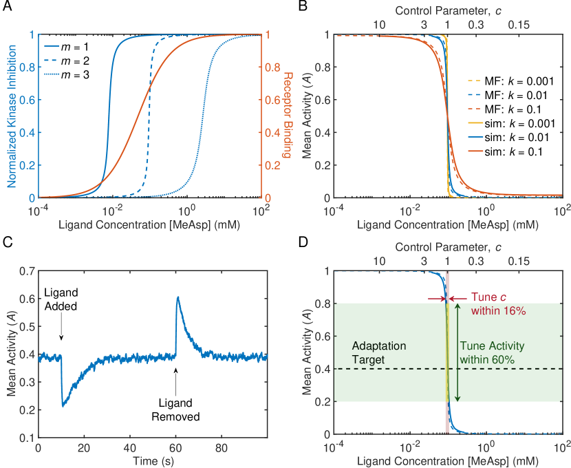
Figure 2: Adaptation and amplification in lattice ultrasensitivity. A) Non-equilibrium coupling between receptors and kinases allows for large gain and adaptation to be absent from receptor binding, but present in kinase activity. Kinase inhibition was calculated using a mean field approximation. B) As $k$ becomes small, the activity dose response curve approaches a step function at $c=1$. Mean field predictions agree with simulations. C) Methylation dynamics allow activity to precisely adapt after an initial fast response to stimulus. The time series is an average of 300 simulations. D) Because methylation is activity dependent and activity is a steep function of the control parameter, adaptation robustly maintains the system near $c=1$, ensuring large gain. If adaptation instead targeted the control parameter, it would be much less robust to variation. For parameter values see Table 1. All mappings from [MeAsp] to $c$ assume $m=2$.

To more quantitatively understand how the LU model achieves large gain, we develop a mean field theory by making the simplifying assumption that the activity of neighboring kinases is well represented by the average activity of all kinases in the lattice. This assumption explicitly ignores any spatial correlation that develops on the lattice. The average kinase activity $A$ then evolves according to:

$$\frac{1}{\nu}\frac{\mathrm{d}A}{\mathrm{d}t}=p([L])(1+e^{g(m)})(1-A)(A+k)\\ -(1-p([L]))(1+e^{-g(m)})A(1-A+k).$$ (4)

We can understand the amplification implied by these kinetics by analyzing the mean-field fixed points. In the limit where $k=0$, both activation and inactivation occur with rates proportional to $A(1-A)$, so that the only fixed points are at $A=0$ and $A=1$. In between these fixed points $A$ increases if $c>1$ and decreases otherwise, so activity becomes switchlike. More generally, at fixed methylation and ligand concentration, the steady state fraction of active kinases only depends on the ratio of switching to spreading, $k$, and the control parameter, $c=c(m,[L])$. It is given by

$$A^{*}=\frac{k(c+1)+1-c-\sqrt{(k(c+1)+1-c)^{2}-4ck(1-c)}}{2(1-c)}.$$ (5)

Plotting $A^{*}$ as a function of the control parameter $c$ shows a sigmoid-like curve with inflection point at $c=1$ where there is precise symmetry between activity and inactivity (Fig. 2B). As we reduce $k$, the curve becomes increasingly steep and switch-like. In the limit where $k\rightarrow 0$, we find that $\mathrm{d}A^{*}/\mathrm{d}c|_{c=1}=(8k)^{-1}$. That is, for small $k$, the slope at the inflection point diverges like $1/k$. This divergence is the source of large gain in our model.

Mean field predictions and lattice simulations agree well (Fig. 2B), but gain is consistently slightly smaller in lattice simulations than in mean field predictions. This is because clustering of kinase activity reduces the effect of spreading relative to switching. Mean field assumes that all kinases have access to every other kinase, but when clustering of like activities occurs, spreading can only occur between kinases at the boundary of a cluster. This effectively reduces the average spreading rate, but spontaneous switching is unaffected. Thus, clustering in the lattice makes spontaneous switching more dominant, effectively increasing $k$ and reducing gain.

The functional form of the steady-state kinase activity $A^{*}$ (Eq. 5) is identical to the fraction of modified substrate in Goldbeter and Koshland’s model of zero-order ultrasensitivity, with the limit $k\rightarrow 0$ in our model corresponding to the case of precise enzyme saturation [39]. Our model displays a form of ultrasensitivity which is mathematically equivalent to zero-order ultrasensitivity but for different structural reasons. In each case, a forward reaction and a separate backward reaction work in opposition on the same substrate, and the system becomes ultrasensitive when the ratio of the forward to backward rate becomes relatively independent of the state of the substrate. For zero-order ultrasensitivity, this relative independence occurs when the competing reactions work at saturation. In our lattice, ultrasensitivity occurs because possible transitions between active and inactive states in either direction always require an active kinase to neighbor an inactive kinase, and thus have the same dependence on average activity. Only spontaneous transitions, occurring at a (much slower) rate $k$, break this relative independence, in exact mathematical analogy to a slight deviation from precisely balanced saturated enzymatic reactions in zero-order ultrasensitivity.

Parameter	Description	Value
$\nu$	Base Spreading Rate	100 s-1
$k_{R}$	Methylation Rate	0.024 s-1
$k_{B}$	Demethylation Rate	0.01 s-1
$k$	Ratio of Switching to Spreading	0.032
$m_{0}$	Crossover Methylation Level	1.8
$\alpha$	Free Energy per Methylation	1.78 kT
$\Delta f_{0}$	Receptor Free Energy Difference	-1.78 kT
$K_{a}$	Dissociation Const. of Activating Receptor	660 $\mu$M
$K_{i}$	Dissociation Const. of Inactivating Receptor	7.4 $\mu$M

Table 1: Simulation Parameters. These values were used in all simulations unless otherwise specified. They were found by fitting data from [6]. See (S1) for details.

Methylation dynamics ensure large gain without fine-tuning

When $k\ll 1$, kinase activity becomes a very steep function of $c$ but only when $c$ is near $1$. To maintain large gain for a wide range of ligand concentrations, the system needs some way to keep $c$ close to 1. The precise adaptation of kinase activity via methylation and demethylation of receptors [41, 42] has exactly the right properties to robustly maintain the system near its switch-like transition:

The standard model for adaptation, well supported by experiments, precisely adapts by methylating only receptors associated with inactive kinases and demethylating only receptors associated with active kinases [26, 19]. We assume a simple quadratic model for the methylation rate of receptors

$$\frac{\mathrm{d}m}{\mathrm{d}t}=k_{R}(1-A)-k_{B}A^{2},$$ (6)

where $k_{R}$ and $k_{B}$ are the rates of methylation and demethylation by CheR and CheB, respectively. The demethylation rate has quadratic dependence on $A$ to account for the activation of CheB via phosphorylation by CheA. However, the qualitative features of our model require only that $\mathrm{d}m/\mathrm{d}t$ is a decreasing function of $A$. Because $\mathrm{d}A/\mathrm{d}t$ is an increasing function of $m$, the fixed point in $m-A$ space will then be stable.

These adaptation dynamics (Eq. 6) only depend on kinase activity $A$, and so the condition that methylation is in steady state ($\mathrm{d}m/\mathrm{d}t=0$) constrains $A^{*}=2/(1+\sqrt{1+4k_{B}/k_{R}})$. As shown above, the constraint that kinase activity is in steady state ($\mathrm{d}A/\mathrm{d}t=0$) yields a relationship between $A^{*}$ and the control parameter c (Eq. 5), so that adaptation dynamics will always bring the system to a fixed value of the control parameter, independent of ligand concentration and methylation level. Thus both $c$ and $A$ perfectly adapt to steady states which are ligand and methylation independent (Fig. 2C), with steady-state methylation levels adapting to changing ligand concentration. Importantly, if $k\ll 1$, the relationship between $A$ and the control parameter $c$ (Eq. 5) is a very steep function. By having feedback from $A$, this system will thus robustly tune to the region where $c$ is near the threshold value of 1: Noise in the levels of adaptation enzymes which effectively change $k_{R}$ and $k_{B}$ will lead to noise in $A^{*}$, but because of the switch-like behavior of $A^{*}$ as a function of $c$, large fluctuations in $A^{*}$ only change $c$ marginally. Thus, when $k\ll 1$ the methylation dynamics achieve not only precise adaptation, but also guarantee large gain without the need for fine-tuning of the control parameter $c$ (Fig. 2D).

These results are reminiscent of feedback proposed in the context of self-organized criticality where the value of the order parameter, the collective output, feeds back onto the control parameter, thereby keeping the system close to its critical point [43, 44]. In our model, this feedback is implemented by adaptation and keeps the control parameter near its critical value ($c=1$), as long as $k$ is small. This robustness is in important contrast to the Ising model where two parameters need to be tuned to find the critical point: the nearest neighbor coupling strength and the activity bias. Similarly to our $c$, the activity bias can be tuned through adaptation. But coupling strength must be separately fine-tuned to its non-zero critical value. In our model, the critical point occurs at $k=0$, which is achievable by a separation of time-scales rather than by precise fine-tuning. This is reminiscent of self-organized critical models that can be understood as remapping a system so that the critical point occurs when a rate is 0 [44].

Self-tuned proximity to the critical point amplifies fluctuations and can cause two-state switching

Large fluctuations in the LU model arise because the critical point which amplifies weak signals also amplifies noise. We can see this by observing the power spectrum of activity fluctuations as we vary $k$ (Fig. 3A). Ligand concentration and methylation level were held constant, so fluctuations are only due to the stochastic dynamics of kinase activity. For large $k$, fluctuations are relatively small, but as $k$ becomes small the size of the fluctuations increases accordingly. In addition, the characteristic frequency of the fluctuations decreases with $k$. To quantify these changes, we extracted the variance and characteristic frequency of the activity fluctuations by fitting the power spectrum to a Lorentz distribution (Fig. 3B). As $k$ decreases, the amplitude and duration of fluctuations increase. This is because the dynamics close to the critical point amplify not only the signal but also the noise and are subject to critical slowing down. Note that the variance saturates at low $k$ because fluctuations become large enough to reach the boundaries of the system and thus cannot continue to grow larger.

In agreement with experimentally observed fluctuations [7, 8], the LU model produces large fluctuations only when activity is brought to an intermediate level through adaptation or fine-tuning of ligand concentration. Indeed, the variance of the fluctuations is sharply peaked in the vicinity of $c=1$ (Fig. 3C). By bringing $c$ close to 1, adaptation thus leads to large fluctuations. To do this without adaption requires fine tuning the ligand concentration. This behavior is reflected in the power spectra. Adapting cells and non-adapting cells with finely tuned ligand concentrations have much larger fluctuations than non-adapting cells without fine tuning (Fig. 3D).

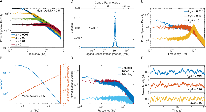
Figure 3: The LU model exhibits large fluctuations. A) Power spectral density of kinase activity fluctuations at constant ligand concentration and methylation, for increasing values of $k$. Black lines show fits to a Lorentzian distribution. B) The characteristic frequency of fluctuations in nonadapting cells is linearly proportional to $k$. The variance shows power law scaling with $k$ when $k$ is large. When $k$ becomes sufficiently small, the variance saturates due to the onset of 2-state switching. C) For non-adapting cells, fluctuations are small (small variance), unless ligand concentration is such that $c$ is near 1. D) Power spectra show very small fluctuations in non-adapting cells without tuned ligand concentrations (mean activity $=0.1$). When cells have a control parameter close to 1 (mean activity $=0.5$), either through adaptation or tuning of ligand concentration, fluctuations are much larger. E) Three different regimes of adapting cells. $k_{R}/k_{B}$ is held constant throughout. When adaptation is much slower than $k$, two distinct timescales are visible in the power spectral density. When adaptation is faster than $k$, the PSD is peaked, indicating the presence of oscillatory behavior. During the transition between these two limits, the PSD appears Lorentzian with a single timescale proportional to $k$. F) Example time series of cells corresponding to the three regimes depicted in E. For parameter values see Table 1. All mappings from [MeAsp] to $c$ assume $m=2$.

Adaptation dynamics also introduce additional features to the fluctuations which depend on the ratio of the (de)methylation rate ($k_{B}$ and $k_{R}$) to the rate of spontaneous switching ($k$). When $k_{R}+k_{B}$ is much less than $k$, the changes in $c$ due to fluctuations in methylation are amplified, adding a second, slower timescale to the power spectrum. When the total adaptation rate is fast relative to $k$, methylation levels respond faster than the kinase activity, leading to oscillations and a peaked power spectrum while lower frequency fluctuations are suppressed. As we shift between these two limits keeping the ratio of methylation and demethylation constant, there is a third region in the middle where the power spectrum again appears Lorentzian (Fig. 3E). These differences, especially the oscillations, are clearly visible in time series of the activity (Fig. 3F). These oscillations might be observable in cells where adaptation enzymes are significantly overexpressed.

When fluctuations are large enough, they can produce the “switch-like” behavior measured in some non-adapting cells. Due to the finite size of the lattice, as fluctuations become large near the critical point, they will eventually drive the system into a state where all the kinases are either active or inactive. When this happens, spreading can no longer occur. The system becomes stuck in this state until a kinase spontaneously switches states and spreading can resume. This ”stickiness” at the edges of the system creates a bimodal distribution recognizable as two-state switching. This can happen in two different ways. At a constant lattice size, reducing $k$ increases the size of fluctuations, eventually leading to two-state switching (Fig. 4A). Alternatively, if we decrease the lattice size while holding $k$ constant, the size of fluctuations (in terms of the total number of kinases changing states) does not change, but because there are fewer kinases, small fluctuations drive the system to saturation more easily (Fig. 4B).

Fluctuations and switching could also be driven by sources of noise extrinsic to receptor-kinase or methylation dynamics. When sufficient external noise is added to the forward or backward rates of enzyme activity in a system with zero-order ultrasensitivity, the system oscillates between a pair of bistable states [45], similar to the two-state switching in E. coli. These extrinsically driven oscillations can also take place in our LU model, where activation and deactivation rates replace forward and backward enzymatic rates in zero-order ultrasensitivity. We can implement external noise in our model by multiplying the kinase activation rate by $e^{x_{OU}}$, where $x_{OU}$ is a variable obeying Ornstein-Uhlenbeck dynamics with zero mean, a defined variance, and a characteristic timescale. Increasing the variance of $x_{OU}$ led to larger fluctuations and eventually bistable oscillations characteristic of two-state switching (Fig. 4C). These extrinsic fluctuations could arise from slow processes not included in our model such as the exchange of receptors and kinases between the lattice and its surroundings, rearrangements of receptors within the lattice [46], or weak interactions with other cellular components. Only about 15% of measured cells exhibited two-state switching, while others were predominantly active or inactive, or exhibited fluctuations between a continuum of states [7]. This implies sources of heterogeneity extrinsic to controlled variables, and it is possible that some of these sources of heterogeneity are themselves dynamic on the timescale of large fluctuations.

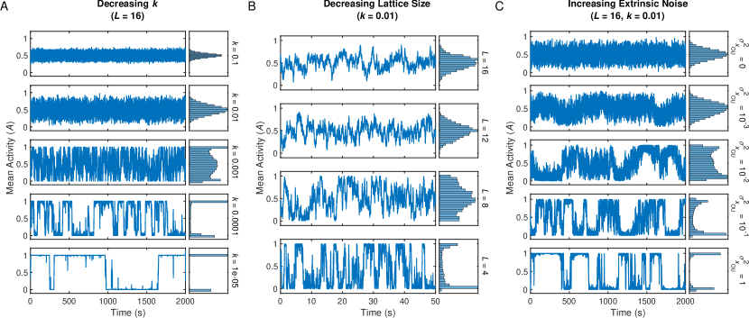
Figure 4: Emergence of two-state switching. A) Simulated time series with mean activity set to 0.5 and decreasing $k$ from top to bottom. As $k$ decreases, fluctuation size and timescales grow. Once fluctuations are large enough to reach the boundaries of the system ($A$ = 0 or $A$ = 1), switching begins to occur. B) As in (A), but now decreasing the linear dimension of the lattice, $L$, from top to bottom. As $L$ decreases, the size of fluctuations relative to the total number of kinases increases. Switching occurs when the system is small enough that the fluctuations reach the boundaries. The x-axis is zoomed in to make high frequency switching clear. C) As in (A), but we have introduced noise into the control parameter. Variance of the noise increases from top to bottom. When the control parameter fluctuations are sufficiently large, the system exhibits two-state switching in what would otherwise be a non-switching system. Here $k$ = 0.01, equivalent to the second plot in (A). For parameter values see Table 1.

Discussion

We have presented a novel lattice model for the large gain observed in E. coli  chemotaxis signaling. Our model naturally explains how both large gain and adaptation can be present at the level of kinase activity, but absent from receptor binding. Our model also recapitulates the large fluctuations and two-state-switching seen in single cell experiments. Finally, unlike other lattice critical models, our model does not require any fine tuned parameters.

The LU model for the origin of large gain is qualitatively different from past models for amplification in chemosensing, but is related to models of ultrasensitivity arising from zeroth order chemical kinetics. Past models of gain mostly contain equilibrium cooperativity, arising from either tight MWC clusters or from nearest neighbor Ising interactions [24, 25, 26, 27, 28, 1, 2, 3, 29, 9]. A recent model put forward in Ref. [38] also uses energy to maintain the kinase layer out of equilibrium from the receptor layer, but with a very different out-of-equilibrium mechanism and with gain arising from neighboring equilibrium interactions. While some functional aspects of that model are similar to LU, the LU model does not require a finely tuned parameter ($J$ in Ref. [38]) to achieve large gain while maintaining fast responses.

Several other biological sensory systems, while mechanistically different from LU, also seem to exploit the divergent susceptibility found near a critical or bifurcation point to amplify weak signals. Hair cells amplify faint sounds in the inner ear by tuning it close to a Hopf bifurcation [47, 48, 49, 50]. We have argued that pit vipers use a saddle-node bifurcation to amplify milli-Kelvin changes in the temperature of their sensory organ into a robust neural response  [51], and that olfactory receptor neurons in fruit flies exploit a bifurcation to reliably extract odor timing information for navigation [52]. In all three cases, it has been argued that order-parameter based feedback, originally introduced in the context of self-organized criticality [43, 44] and bistability [53, 54], allows the system to maintain proximity to the critical or bifurcation point without the need for fine-tuning. In our model, this feedback from the order parameter back onto the control parameter is implemented by the activity dependence of methylation dynamics [41, 55, 56].

The critical point in our model reproduces the most salient features of fluctuations measured in single cells: large fluctuations in adapting cells, and two-state switching in non-adapting cells with finely-tuned ligand concentrations [7, 8]. The magnitude of these fluctuations is larger than expected in MWC-like models where kinases act independently or in small groups. Indeed, such large fluctuations, and especially two-state switching, are difficult to reconcile with any model that does not include a lattice critical point. Both our model and Ising models contain such a critical point, and, in the absence of adaptation, require fine-tuning ligand concentration or methylation to generate large fluctuations. In either case, however, it’s not clear how the same dynamics could generate both a very fast response to changing ligand and the very slow fluctuations seen in measurements. Thus, it may be that the long timescale fluctuations are best understood as arising from fluctuating variables extrinsic to our model. Indeed, almost any slow process, such as the rearrangement of receptors within the lattice [46], could create noise in the control parameter responsible for driving the fluctuations.

Additional features of the LU model that distinguish it from other models can be traced directly to its non-equilibrium dynamics. Because the coupling from receptors to kinase activity is non-reciprocal, receptors can have meaningfully different states than their associated kinases. These differences, apparent in both adaptation and gain, have been observed experimentally [30, 31, 57] and are inconsistent with Ising and MWC models [32]. Other non-equilibrium models have been proposed to accommodate these differences between receptor binding and kinase activity, but they do not address observed fluctuations [32]. A more recent model addresses distinct receptors and fluctuations simultaneously by combining a non-equilibrium reaction cycle within core signaling units with an Ising-like coupling between neighboring units [38]. However, like equilibrium Ising models, this model still requires fine-tuning of the coupling parameter to maximize susceptibility.

One observation we do not explain in this paper, but is described in Ref. [38], is the asymmetry observed in cells exhibiting two-state switching. The observed mean time to switch from inactive to active is faster (4.3s) than the reverse (6.1s) [37]. Two-state switching in the LU model via intrinsic fluctuations (Fig. 4A,B) cannot capture this behavior. When $c=1$ the dynamics are entirely symmetric, and away from $c=1$, any asymmetry would necessarily be correlated with the activity bias through $c$. However, if switching is due to extrinsic noise in $c$, specifically through fluctuations in the spreading rate of activity but not inactivity, this asymmetry would arise. Introducing other sources of asymmetry to the LU model, perhaps through different rates for spontaneous activation and inactivation, could produce similar results.

Experiments place subtle constraints on the dependence of the dynamics on ligand concentration and methylation. Simultaneous measurements of receptor binding and kinase activity show that kinase activity can respond as strongly to changes from 1 to 2 percent of receptors bound as to changes from 98 to 99 percent bound [31]. In the former case the bound fraction doubles, while the unbound decreases by just 1 percent, while in the latter case the reverse is true. This seems to require one mechanism to measure the number of bound receptors, and another to measure the number of unbound ones. We represent these mechanisms by making activation of kinases proportional to the probability $p$ that a receptor is activating, while inactivation is proportional to $(1-p)$. We chose the methylation dependence of the activation and deactivation rates so that the response speed is mostly independent of ligand concentration and methylation after adaptation (see SI).

Our model’s non-equilibrium nature makes a range of predictions that may be tested in future experiments. Because an activating receptor completely restricts its associated kinase from becoming inactive, the activation of that kinase is irreversible and requires infinite dissipation. By relaxing this restriction, it might be possible to develop relationships between various signaling characteristics (response time, gain, variance, etc.) and the dissipation in the system, similar to what has been done for other non-equilibrium models [32, 38]. These relationships might be testable through experiments which restrict the free energy available via ATP hydrolysis. While not necessarily specific to the LU model, we also expect that balanced over-expression of adaptation enzymes CheR and CheB should lead to oscillations in kinase activity in steady state (Fig. 3E,F).

States and transitions between them have a different meaning in the LU model than in traditional equilibrium models. In Ising and MWC models, states can be understood as distinct coarse-grainings of allosteric protein configurations. Transitions between states are driven by thermal fluctuations and modulated by energetic interactions. In the LU model, kinase states are instead related to chemical modification, likely phosphorylation of the P1 domain, and changes are driven by far from equilibrium enzymatic reactions.

There are several plausible mechanisms for implementing non-equilibrium spreading, all of which must eventually use energy from ATP hydrolysis. It is possible that the energy from phosphorylation pushes CheW or CheA-P5 into a transient high energy configuration which catalyzes a like reaction on a neighboring kinase. Alternatively, spreading could represent a direct interaction between neighboring kinases, dependent on their phosphorylation state. While CheA P3-P5 domains are rigidly attached to the signaling lattice, the P1 domain is attached only by a long flexible linker region, and the number of amino acids in the linker suggests it may be long enough to reach between neighboring core units to facilitate these interactions [20, 21, 22, 23, 4]. Productive interactions might spread activity, for example through phosphorylation, while unproductive interactions spread inactivity. There is evidence of both productive and unproductive binding sites on the CheA [58, 59, 60, 12].

Future experiments could test for these linker-mediated interactions. Shortening the linkers should make interactions between neighboring kinasese less likely. This could reduce gain, but might entirely stop signal transduction first. As for lengthening linkers, experiments have already shown that mutants whose P1 and P2 domain are entirely separate from the lattice and soluble in the cytoplasm are still able to chemotax [61], but quantitative probes of signaling activity in these cells have not been performed. Some mutations in the adaptor CheW (CheW-X2) prevent lattice formation and reduce gain at the kinase level [62, 63]. This has been interpreted to imply that there is allosteric coupling mediated directly through the lattice [63], but it could be that core units are too spatially separated from each other for their linkers to reach in disrupted lattices. Perhaps mutants with soluble P1-P2 domains can partially rescue large gain in CheW-X2 mutants without restoring the lattice. Intriguingly Vibrio has far fewer and therefore sparser CheA [64], but their linker is significantly longer [21, 22, 23], potentially allowing CheAs to interact over longer distances. Although the specific molecular mechanisms underlying the LU model are underconstrained, the likely mechanisms are quite different from those found in equilibrium models and suggest new areas for future experiments.

S1 Determining Parameter Values

S1.1 Fitting Dose Response Curves

We fit our model to dose response curves measured in Ref. [6] for various methylation mutants (EEEE, QEEE, QEQE, QQQE, QQQQ, QEmQQ, QEmQEm, EmEmEmEm). EEEE and EmEmEmEm were ignored in the initial fitting process because their activities were constant at 0 and 1, respectively, and thus could not be fit directly. After normalizing the remaining dose response curves by their mean activity, we used MATLAB’s nonlinear least-squares curve-fitting function to simultaneously fit each dose response curves to the mean-field steady state activity for our model (Eq. S2).

$$c(m,[L])=\frac{p([L])}{1-p([L])}e^{g(m)}$$ (S1)

$$A^{*}=\frac{k(c+1)+1-c-\sqrt{(k(c+1)+1-c)^{2}-4ck(1-c)}}{2(1-c)}.$$ (S2)

$g(m)$ was allowed to vary between mutants since they each had different methylation levels. All other parameters were held constant between mutants. Fits to dose response curves are shown in Fig. S1A.

From these fits, we found $k$, $K_{i}$, $K_{a}$, $\Delta f0$, and a value of $g(m)$ for each mutant. To find $\alpha$ and $m_{0}$, we first want to find $g(m)$ for EEEE and EmEmEmEm mutants. $g(m)$ for mutants containing only glutamate (E) and glutamine (Q) fell on a reasonable straight line, as did mutants containing only glutamine (Q) and methylated glutamate (Em) (Fig. S1B), so $g(m)_{\mathrm{EEEE}}$ and $g(m)_{\mathrm{EmEmEmEm}}$ were determined by extrapolation of these two lines. $m_{0}=g(m)_{\mathrm{EEEE}}$, and $\alpha$ is just the slope of the line between $g(m)_{\mathrm{EEEE}}$ and $g(m)_{\mathrm{EmEmEmEm}}$. All these parameter values are in Table S1.

Parameter	Description	Values w/ Linear Methylation	Values w/ free $g(m)$
$k$	Ratio of Switching to Spreading	0.032	0.048
$m_{0}$	Crossover Methylation	1.80	1.44
$\alpha$	Free Energy per Methylation	1.78 kT	1.95 kT
$\Delta f_{0}$	Receptor Free Energy Difference	-1.78 kT	-1.78 kT
$K_{a}$	Dissociation Const. of Activating Receptor	660 $\mu$M	683 $\mu$M
$K_{i}$	Dissociation Const. of Inactivating Receptor	7.4 $\mu$M	5 $\mu$M

Table S1: Parameters found from fitting data from Ref. [6]

Although the linear form of $g(m)$, if assign each methylation mutant a specific value of $m$ (EEEE: $m=0$, QEEE: $m=0.5$, QEQE: $m=1$, QQQE: $m=1.5$, QQQQ: $m=2$, QEmQQ: $m=2.5$, QEmQEm: $m=3$, EmEmEmEm: $m=4$) and plot the predicted dose response curves against the data, the dose response curve for QEEE and QEmQEm mutants show poor agreement with the data for small and large ligand concentrations, respectively (Fig. S1C). This is because large parts of these curve lie at intermediate activities ($c\approx 1$) where they are very sensitive to the small differences between the fit $g(m)$ and the $g(m)$ based on linear methylation.

To address this, we again fit the data. This time, rather than fitting $g(m)$ freely, we enforced the linear form $g(m)=\alpha(m-m_{0})$ assigning each mutant the same $m$ as above, and fit for $\alpha$ and $m_{0}$ directly (Table S1). When assuming the linear form of $g(m)$ used in the paper and simulations, these parameters fit the data better than those derived from fitting with unconstrained $g(m)$ (Fig. S1D). We used these new throughout the paper.

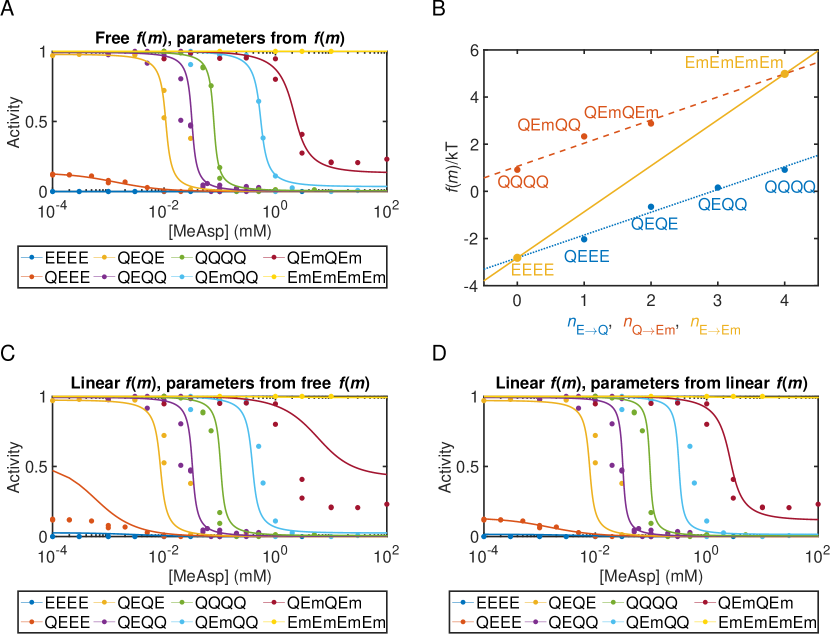
Figure S1: Fitting experimental dose response curves. A) Fits allowing free choice for $g(m)$ agree well experimental data. B) Values of $g(m)$ plotted against modification states, show an approximately linear dependence on the modification state C) If we assume that $g(m)$ is linear in $m$ and plot the predicted curves based on $\alpha$ and $m_{0}$ derived from the fit in (A), the fit is less good. D) After refitting with the explicit assumption that $g(m)$ is linear, predictions agree much better with the data. All data in this figure is taken from Ref. [6]

S1.2 Finding the remaining parameters

After fitting the dose response curves, we still need to determine the base spreading rate $\nu$ and the methylation and demethylation rates $k_{R}$ and $k_{B}$. The steady state activity level after adaptation, $\bar{A}=2/(1+\sqrt{1+4k_{B}/k_{R}})$, determines the ratio $k_{R}/k_{B}$. We chose $\bar{A}=0.3$ in rough agreement with the average of cells from Ref. [33], corresponding to $k_{R}/k_{B}=2.4$. The total of the (de)methylation rates, $k_{R}+k_{B}$, determines the adaptation timescale, which is roughly 10 seconds [33]. After simulating the response of adapting cells to a 10% change in ligand concentration for a variety of values, we found that $k_{R}+k_{B}=0.034\mathrm{s}^{-}1$ roughly corresponds to an adaptation timescale of 10 s. Because of significant variability between individual cells, a more precise fitting procedure for the (de)methylation rates would provide meaningfully better information.

Because the response timescale of kinase activity is smaller than the time resolution available from FRET microscopy [33], it cannot be effective constrained by FRET measurements. This, in turn, means that the base spreading rate $\nu$ is also poorly constrained, with the only requirement being that our system responds faster than the resolution of FRET microscopy, roughly 500 ms. We chose $\nu=100~{}\mathrm{Hz}$, comfortably above this minimum rate.

These additional parameters are summarized in Table S2.

Parameter	Description	Value
$\nu$	Base Spreading Rate	100 s-1
$k_{R}$	Methylation Rate	0.024 s-1
$k_{B}$	Demethylation Rate	0.01 s-1

Table S2: Additional parameter values chosen for use in our model.

S2 Description of Simulations

S2.1 Setup and Initialization

In our simulation, core signaling complexes (CSCs) are located on the sites of a square lattice. There are two values associated with each CSC on the lattice: a kinases activity ($A$), and a methylation level ($m$). The kinase activity takes a value of 0 or 1, corresponding the inactive or active state, respectively. The methylation level takes a value between 0 and 4. Since there are 12 receptors (2 trimers of dimers) in each CSC, we discretize methylation levels into steps of $dm=1/12$, corresponding to the methylation of a single site of one receptor. A methylation level of 0 or 4 means that every receptor in the CSC is either fully demethylated or methylated. There is also a value $p$ associated with the state of the receptor in each CSC. We assume that the dynamics of the receptor state are in fast equilibrium relatively to the other dynamics of the system, so rather than take a value of 0 or 1 corresponding to the inactivating or activating states, it takes the average state, $p$, somewhere between 0 and 1.

$$p([L])=(1+e^{\Delta f([L])})^{-1}.$$ (S3)

$$\Delta f([L])=\Delta f_{0}+\mathrm{log}\left(\frac{1+[L]/K_{i}}{1+[L]/K_{a}}\right)$$ (S4)

Because this model only accounts for a single type of receptor, and all the receptors are in fast equilibrium, we treat the value of the receptor state as a deterministic global variable rather than a stochastic variable with a different value at each CSC.

To initialize the simulation with adaptation, the kinase activity and methylation level of each CSC is determined randomly. The receptor state is determined based on the initial ligand concentration. If we are simulating an non-adapting mutant (e.g. QEQE), initialization of the kinase activity and the receptor state occurs as above, but the methylation level of each CSC is set to a constant value that is determined by the mutant in question.

S2.2 Dynamics

Dynamics are then simulated using a Gillespie algorithm [40] with unique reactions for each CSC. The propensity for reactions at the $i$th CSC are given by the following: An inactive kinase becoming active

$$r_{0\rightarrow 1}^{A_{i}}=p(1+e^{m_{0}+\alpha m_{i}})(k+\frac{1}{4}\sum_{j\in n.n.}A_{j}),$$ (S5)

where $m$ is the methylation level of the CSC, other variables are defined as in the main paper, and the sum is over the activity values of nearest neighbor kinases. The propensity for active kinases to become inactive is given by

$$r_{1\rightarrow 0}^{A_{i}}=(1-p)(1+e^{-m_{0}+\alpha m_{i})})((k+1-\frac{1}{4}\sum_{j\in n.n.}A_{j}).$$ (S6)

The propensity to increase the methylation by $dm$ is given by

$$r^{m_{i}}_{+dm}=k_{R}(1-A_{i}).$$ (S7)

The propensity to decrease the methylation by $dm$ is given by

$$r^{m_{i}}_{-dm}=k_{B}A_{i}\frac{1}{N}\sum_{j=1}^{N}A_{j}.$$ (S8)

Here, the sum is over every lattice site, making the demethylation rate proportional to both the single site activity and the average over the entire lattice. This accounts for the activation of CheB via phosphorylation by CheA.

Sometimes, rather than simulate the lattice at a specific methylation level and/or ligand concentration, it is convenient to just set the control parameter $c=e^{m_{0}+\alpha m_{i}}p/(1-p)$, which combines the influence of methylation and ligand into a single parameter. In this case, the propensity for methylation and demethylation are unchanged, while those of activation and inactivation of kinases becomes

$$r_{0\rightarrow 1}^{A_{i}}=\frac{c+1}{2}(k+\frac{1}{4}\sum_{j\in n.n.}A_{j}),$$ (S9)

and

$$r_{1\rightarrow 0}^{A_{i}}=\frac{\frac{1}{c}+1}{2}(k+1-\frac{1}{4}\sum_{j\in n.n.}A_{j}).$$ (S10)

The prefactors were chosen to correspond with the case where $p=0.5$. Because the total rates depend slightly on $p$ when $c\neq 1$, we need to choose a specific value of $p$ when running these simulations.

In a traditional Gillespie algorithm, all of these individual propensities are calculated at the beginning of each step of the simulation. Then a single reaction is chosen to take place, with the probability for a given reaction to be chosen is proportional to its propensity. The amount of time that passes between each reaction would chosen from an exponential distribution whose timescale is equal to the inverse of the sum of all of the reaction propensities.

In order to speed up simulation times, a form of tau leaping was implemented. Rather than recalculate all the propensities after each reaction, we perform multiple reactions drawing from the same propensity function. The number of reactions performed was chosen to be

$$n=0.1\textrm{ min}(\sum_{j}A_{j},N-\sum_{j}A_{j}),$$ (S11)

rounded up. This guarantees that the total number of active or inactive kinases will not change by more than 10 percent, ensuring that our approximation of a constant propensity function is good for all the reactions. The timestep is then corresponding increased by a factor of $n$.

The units in our simulation are defined so that the spreading rate of activity at $c=1$ is equal to 1. Thus one unit of time in the simulation is equal to 1/$s$ seconds, where $s$ is the spreading rate in units inverse seconds.

Before taking data, if adaptation is occurring the model is run for $3/(k_{R}+k_{B})$ seconds in order to equilibrate. If adaptation is not occurring (i.e $k_{R}=k_{B}=0$) the simulation is run for 100 seconds to equilibrate.

Once the system has equilibrated, we run through whatever experimental protocol we need to. A protocol is defined as a series of ligand concentrations and a length of time the system experiences each ligand concentration in that series. The ligand concentration chosen for equilibration should be the same as the first ligand concentration in the series. The system is run for the specified amount of time at that concentration, then changed to the next one, until the protocol is complete.

S2.3 Resampling

At this point, the model has output a time series of methylation levels and kinase activities, but the spacing between timepoints is non-uniform. For ease of analysis, we then resample the data at 100 Hz using MATLAB’s resample function to create a uniformly sampled time series (Fig. S2). From there, it is easy to calculate the power spectrum, or average over many different realizations of the same protocol.

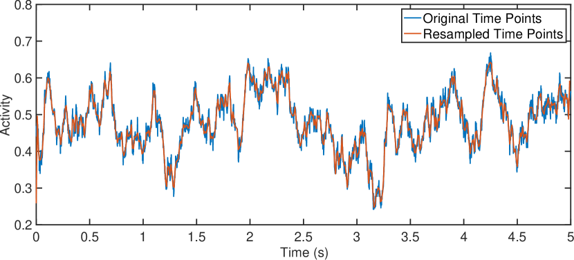
Figure S2: A comparison of original and resampled data. Results are identical, except on timescale less than 0.1 seconds, which are not probe-able using current FRET techniques.

S2.4 Implementing External Noise

To implement sources of noise in the control parameter that are external to our model, we multiplied $r_{0\rightarrow 1}^{A_{i}}$ by an additional term, $e^{x_{\mathrm{OU}}}$. ${x_{\mathrm{OU}}}$ is described by an Ornstein-Uhlenbeck process with a relaxation time $\tau$ and a noise scale $D$. It’s value is updated at every time-step of the simulation obeying the following rule:

$$x_{\mathrm{OU}}(t+dt)=x_{\mathrm{OU}}(t)\left(1-\frac{dt}{\tau}\right)+D\mathrm{N(0,1)}\sqrt{dt}.$$ (S12)

Here, N(0,1) denotes a random variable drawn from a normal distribution with mean 0 and variance 1.

S3 Dependence of Response Times on Receptor State

We wanted the response speed of the LU model to be roughly independent of ligand concentration once the system reached its adapted steady state activity $\bar{A}=A^{*}(\bar{c})$. Since the response rate is proportional to sum of the activation and deactivation rates, and ligand concentration only enters into the dynamics through the average receptor state $p$, this is equivalent to wanting the sum of activation and deactivation rates to have minimal dependence on $p$ when $c$ is held constant.

The sum of activation and deactivation rates is

$$k_{\mathrm{response}}\propto(1+e^{g(m)})p+(1+e^{-g(m)})(1-p).$$ (S13)

We also know that

$$c=\frac{(1+e^{g(m)})p}{(1+e^{-g(m)})(1-p)}=e^{g(m)}\frac{p}{1-p}.$$ (S14)

Solving for $e^{g(m)}$ in Eq. S14 and substituting it into Eq. S13, we find

$$k_{\mathrm{response}}\propto\left(1+\frac{c(1-p)}{p}\right)p+\left(1+\frac{p}{c(1-p)}\right)(1-p),$$ (S15)

which simplifies to

$$k_{\mathrm{response}}\propto c(1-p)+(1+\frac{p}{c}).$$ (S16)

If we take the ratio of $k_{\mathrm{response}}$ when $p=0$ to $k_{\mathrm{response}}$ when $p=1$, we find that

$$\frac{k_{\mathrm{response}}(p=0)}{k_{\mathrm{response}}(p=1)}=c.$$ (S17)

That means that, for different values of $p$, and thus ligand concentration, the response rate can change by at most a factor of $c$. Since, as discussed in the main text, $\bar{c}$ is should always be close to 1, the response rate after adaptation should be very close to independent of the ligand concentration adapted to.

References

- [1] Victor Sourjik and Howard C. Berg “Functional Interactions between Receptors in Bacterial Chemotaxis” In Nature 428.6981, 2004, pp. 437–441 DOI: 10.1038/nature02406
- [2] Ganhui Lan, Sonja Schulmeister, Victor Sourjik and Yuhai Tu “Adapt Locally and Act Globally: Strategy to Maintain High Chemoreceptor Sensitivity in Complex Environments” In Molecular Systems Biology 7.1, 2011, pp. 475 DOI: 10.1038/msb.2011.8
- [3] Yuhai Tu “Quantitative Modeling of Bacterial Chemotaxis: Signal Amplification and Accurate Adaptation” In Annual Review of Biophysics 42.1, 2013, pp. 337–359 DOI: 10.1146/annurev-biophys-083012-130358
- [4] Jacki P. Goldman, Matthew D. Levin and Dennis Bray “Signal Amplification in a Lattice of Coupled Protein Kinases” In Molecular BioSystems 5.12, 2009, pp. 1853 DOI: 10.1039/b903397a
- [5] V. Sourjik and H.. Berg “Receptor Sensitivity in Bacterial Chemotaxis” In Proceedings of the National Academy of Sciences 99.1, 2002, pp. 123–127 DOI: 10.1073/pnas.011589998
- [6] Thomas S Shimizu, Yuhai Tu and Howard C Berg “A Modular Gradient-sensing Network for Chemotaxis in Escherichia Coli Revealed by Responses to Time-varying Stimuli” In Molecular Systems Biology 6.1, 2010, pp. 382 DOI: 10.1038/msb.2010.37
- [7] Johannes M Keegstra et al. “Phenotypic Diversity and Temporal Variability in a Bacterial Signaling Network Revealed by Single-Cell FRET” In eLife 6, 2017, pp. e27455 DOI: 10.7554/eLife.27455
- [8] Remy Colin, Christelle Rosazza, Ady Vaknin and Victor Sourjik “Multiple Sources of Slow Activity Fluctuations in a Bacterial Chemosensory Network” In eLife 6, 2017, pp. e26796 DOI: 10.7554/eLife.26796
- [9] K. Kamino et al. “Adaptive Tuning of Cell Sensory Diversity without Changes in Gene Expression” In Science Advances 6.46, 2020, pp. eabc1087 DOI: 10.1126/sciadv.abc1087
- [10] Jeremy Philippe Moore, Keita Kamino and Thierry Emonet “Non-Genetic Diversity in Chemosensing and Chemotactic Behavior” In International Journal of Molecular Sciences 22.13, 2021, pp. 6960 DOI: 10.3390/ijms22136960
- [11] J.. Moore et al. “Signal Integration and Adaptive Sensory Diversity Tuning in Escherichia coli Chemotaxis” In Cell Systems, 2024
- [12] C. Cassidy et al. “Structure of the Native Chemotaxis Core Signaling Unit from Phage E-protein Lysed E. Coli Cells” In mBio 14.5, 2023, pp. e00793–23 DOI: 10.1128/mbio.00793-23
- [13] Snezana Djordjevic and Ann M Stock “Crystal Structure of the Chemotaxis Receptor Methyltransferase CheR Suggests a Conserved Structural Motif for Binding S-adenosylmethionine” In Structure 5.4, 1997, pp. 545–558 DOI: 10.1016/S0969-2126(97)00210-4
- [14] Snezana Djordjevic et al. “Structural Basis for Methylesterase CheB Regulation by a Phosphorylation-Activated Domain” In Proceedings of the National Academy of Sciences 95.4 National Acad Sciences, 1998, pp. 1381–1386
- [15] Ariane Briegel et al. “Universal Architecture of Bacterial Chemoreceptor Arrays” In Proceedings of the National Academy of Sciences 106.40, 2009, pp. 17181–17186 DOI: 10.1073/pnas.0905181106
- [16] Jun Liu et al. “Molecular Architecture of Chemoreceptor Arrays Revealed by Cryoelectron Tomography of Escherichia Coli Minicells” In Proceedings of the National Academy of Sciences 109.23, 2012 DOI: 10.1073/pnas.1200781109
- [17] Ariane Briegel et al. “New Insights into Bacterial Chemoreceptor Array Structure and Assembly from Electron Cryotomography” In Biochemistry 53.10, 2014, pp. 1575–1585 DOI: 10.1021/bi5000614
- [18] Mingshan Li and Gerald L. Hazelbauer “Core Unit of Chemotaxis Signaling Complexes” In Proceedings of the National Academy of Sciences 108.23, 2011, pp. 9390–9395 DOI: 10.1073/pnas.1104824108
- [19] John S. Parkinson, Gerald L. Hazelbauer and Joseph J. Falke “Signaling and Sensory Adaptation in Escherichia Coli Chemoreceptors: 2015 Update” In Trends in Microbiology 23.5, 2015, pp. 257–266 DOI: 10.1016/j.tim.2015.03.003
- [20] T B Morrison and J S Parkinson “Liberation of an Interaction Domain from the Phosphotransfer Region of CheA, a Signaling Kinase of Escherichia Coli.” In Proceedings of the National Academy of Sciences 91.12, 1994, pp. 5485–5489 DOI: 10.1073/pnas.91.12.5485
- [21] John Jumper et al. “Highly Accurate Protein Structure Prediction with AlphaFold” In Nature 596.7873, 2021, pp. 583–589 DOI: 10.1038/s41586-021-03819-2
- [22] Mihaly Varadi et al. “AlphaFold Protein Structure Database: Massively Expanding the Structural Coverage of Protein-Sequence Space with High-Accuracy Models” In Nucleic Acids Research 50.D1, 2022, pp. D439–D444 DOI: 10.1093/nar/gkab1061
- [23] Mihaly Varadi et al. “AlphaFold Protein Structure Database in 2024: Providing Structure Coverage for over 214 Million Protein Sequences” In Nucleic Acids Research 52.D1, 2024, pp. D368–D375 DOI: 10.1093/nar/gkad1011
- [24] Dennis Bray, Matthew D Levin and Carl J Morton-Firth “Receptor Clustering as a Cellular Mechanism to Control Sensitivity” In Nature 393.6680 Nature Publishing Group UK London, 1998, pp. 85–88
- [25] T… Duke and D. Bray “Heightened Sensitivity of a Lattice of Membrane Receptors” In Proceedings of the National Academy of Sciences 96.18, 1999, pp. 10104–10108 DOI: 10.1073/pnas.96.18.10104
- [26] Carl Jason Morton-Firth, Thomas Simon Shimizu and Dennis Bray “A Free-Energy-Based Stochastic Simulation of the Tar Receptor Complex” In Journal of molecular biology 286.4 Elsevier, 1999, pp. 1059–1074
- [27] Thomas S. Shimizu, Sergej V. Aksenov and Dennis Bray “A Spatially Extended Stochastic Model of the Bacterial Chemotaxis Signalling Pathway” In Journal of Molecular Biology 329.2, 2003, pp. 291–309 DOI: 10.1016/S0022-2836(03)00437-6
- [28] Bernardo A. Mello and Yuhai Tu “Quantitative Modeling of Sensitivity in Bacterial Chemotaxis: The Role of Coupling among Different Chemoreceptor Species” In Proceedings of the National Academy of Sciences 100.14, 2003, pp. 8223–8228 DOI: 10.1073/pnas.1330839100
- [29] Monica L. Skoge, Robert G. Endres and Ned S. Wingreen “Receptor-Receptor Coupling in Bacterial Chemotaxis: Evidence for Strongly Coupled Clusters” In Biophysical Journal 90.12, 2006, pp. 4317–4326 DOI: 10.1529/biophysj.105.079905
- [30] Mikhail N. Levit and Jeffry B. Stock “Receptor Methylation Controls the Magnitude of Stimulus-Response Coupling in Bacterial Chemotaxis” In Journal of Biological Chemistry 277.39, 2002, pp. 36760–36765 DOI: 10.1074/jbc.M204325200
- [31] Divya N. Amin and Gerald L. Hazelbauer “Chemoreceptors in Signalling Complexes: Shifted Conformation and Asymmetric Coupling: Chemoreceptors in Signalling Complexes” In Molecular Microbiology 78.5, 2010, pp. 1313–1323 DOI: 10.1111/j.1365-2958.2010.07408.x
- [32] David Hathcock et al. “A Nonequilibrium Allosteric Model for Receptor-Kinase Complexes: The Role of Energy Dissipation in Chemotaxis Signaling” In Proceedings of the National Academy of Sciences 120.42, 2023, pp. e2303115120 DOI: 10.1073/pnas.2303115120
- [33] H.. Mattingly, K. Kamino, B.. Machta and T. Emonet “Escherichia Coli Chemotaxis Is Information Limited” In Nature Physics 17.12, 2021, pp. 1426–1431 DOI: 10.1038/s41567-021-01380-3
- [34] Ekaterina Korobkova et al. “From Molecular Noise to Behavioural Variability in a Single Bacterium” In Nature 428.6982, 2004, pp. 574–578 DOI: 10.1038/nature02404
- [35] Heungwon Park et al. “Interdependence of Behavioural Variability and Response to Small Stimuli in Bacteria” In Nature 468.7325, 2010, pp. 819–823 DOI: 10.1038/nature09551
- [36] Heungwon Park, Panos Oikonomou, Calin C. Guet and Philippe Cluzel “Noise Underlies Switching Behavior of the Bacterial Flagellum” In Biophysical Journal 101.10, 2011, pp. 2336–2340 DOI: 10.1016/j.bpj.2011.09.040
- [37] Johannes M Keegstra et al. “Near-Critical Tuning of Cooperativity Revealed by Spontaneous Switching in a Protein Signalling Array”, 2022 DOI: 10.1101/2022.12.04.518992
- [38] David Hathcock, Qiwei Yu and Yuhai Tu “Time-Reversal Symmetry Breaking in the Chemosensory Array: Asymmetric Switching and Dissipation-Enhanced Sensing” arXiv, 2023 arXiv:2312.17424 [cond-mat, physics:physics, q-bio]
- [39] A Goldbeter and D E Koshland “An Amplified Sensitivity Arising from Covalent Modification in Biological Systems.” In Proceedings of the National Academy of Sciences 78.11, 1981, pp. 6840–6844 DOI: 10.1073/pnas.78.11.6840
- [40] Daniel T Gillespie “Exact Stochastic Simulation of Coupled Chemical Reactions” In The journal of physical chemistry 81.25 ACS Publications, 1977, pp. 2340–2361
- [41] N. Barkai and S. Leibler “Robustness in Simple Biochemical Networks” In Nature 387.6636, 1997, pp. 913–917 DOI: 10.1038/43199
- [42] Uri Alon, Michael G Surette, Naama Barkai and Stanislas Leibler “Robustness in Bacterial Chemotaxis” In Nature 397.6715 Nature Publishing Group UK London, 1999, pp. 168–171
- [43] Didier Sornette “Critical Phase Transitions Made Self-Organized : A Dynamical System Feedback Mechanism for Self-Organized Criticality” In Journal de Physique I 2.11, 1992, pp. 2065–2073 DOI: 10.1051/jp1:1992267
- [44] Didier Sornette, Anders Johansen and Ivan Dornic “Mapping Self-Organized Criticality onto Criticality” In Journal de Physique I 5.3, 1995, pp. 325–335 DOI: 10.1051/jp1:1995129
- [45] Michael Samoilov, Sergey Plyasunov and Adam P. Arkin “Stochastic Amplification and Signaling in Enzymatic Futile Cycles through Noise-Induced Bistability with Oscillations” In Proceedings of the National Academy of Sciences 102.7, 2005, pp. 2310–2315 DOI: 10.1073/pnas.0406841102
- [46] Vered Frank and Ady Vaknin “Prolonged Stimuli Alter the Bacterial Chemosensory Clusters: Stimuli Alter Chemosensory Clusters” In Molecular Microbiology 88.3, 2013, pp. 634–644 DOI: 10.1111/mmi.12215
- [47] Sébastien Camalet, Thomas Duke, Frank Jülicher and Jacques Prost “Auditory Sensitivity Provided by Self-Tuned Critical Oscillations of Hair Cells” In Proceedings of the National Academy of Sciences 97.7, 2000, pp. 3183–3188 DOI: 10.1073/pnas.97.7.3183
- [48] Yong Choe, Marcelo O. Magnasco and A.. Hudspeth “A Model for Amplification of Hair-Bundle Motion by Cyclical Binding of Ca 2+ to Mechanoelectrical-Transduction Channels” In Proceedings of the National Academy of Sciences 95.26, 1998, pp. 15321–15326 DOI: 10.1073/pnas.95.26.15321
- [49] V.. Eguíluz et al. “Essential Nonlinearities in Hearing” In Physical Review Letters 84.22, 2000, pp. 5232–5235 DOI: 10.1103/PhysRevLett.84.5232
- [50] A.. Hudspeth, Frank Jülicher and Pascal Martin “A Critique of the Critical Cochlea: Hopf—a Bifurcation—Is Better Than None” In Journal of Neurophysiology 104.3, 2010, pp. 1219–1229 DOI: 10.1152/jn.00437.2010
- [51] Isabella R. Graf and Benjamin B. Machta “A Bifurcation Integrates Information from Many Noisy Ion Channels and Allows for Milli-Kelvin Thermal Sensitivity in the Snake Pit Organ” In Proceedings of the National Academy of Sciences 121.6, 2024, pp. e2308215121 DOI: 10.1073/pnas.2308215121
- [52] K. Choi et al. “Bifurcation enhances temporal information encoding in the olfactory periphery” In bioRxiv, 2024
- [53] Serena di Santo, Raffaella Burioni, Alessandro Vezzani and Miguel A. Muñoz “Self-Organized Bistability Associated with First-Order Phase Transitions” In Physical Review Letters 116.24, 2016, pp. 240601 DOI: 10.1103/PhysRevLett.116.240601
- [54] Victor Buendía, Serena di Santo, Juan A. Bonachela and Miguel A. Muñoz “Feedback Mechanisms for Self-Organization to the Edge of a Phase Transition” In Frontiers in Physics 8, 2020, pp. 333 DOI: 10.3389/fphy.2020.00333
- [55] Tau-Mu Yi, Yun Huang, Melvin I. Simon and John Doyle “Robust Perfect Adaptation in Bacterial Chemotaxis through Integral Feedback Control” In Proceedings of the National Academy of Sciences 97.9, 2000, pp. 4649–4653 DOI: 10.1073/pnas.97.9.4649
- [56] Stephanie K. Aoki et al. “A Universal Biomolecular Integral Feedback Controller for Robust Perfect Adaptation” In Nature 570.7762, 2019, pp. 533–537 DOI: 10.1038/s41586-019-1321-1
- [57] Ady Vaknin and Howard C. Berg “Physical Responses of Bacterial Chemoreceptors” In Journal of Molecular Biology 366.5, 2007, pp. 1416–1423 DOI: 10.1016/j.jmb.2006.12.024
- [58] Damon J. Hamel et al. “Chemical-Shift-Perturbation Mapping of the Phosphotransfer and Catalytic Domain Interaction in the Histidine Autokinase CheA from Thermotoga Maritima ” In Biochemistry 45.31, 2006, pp. 9509–9517 DOI: 10.1021/bi060798k
- [59] Alise R. Muok, Ariane Briegel and Brian R. Crane “Regulation of the Chemotaxis Histidine Kinase CheA: A Structural Perspective” In Biochimica et Biophysica Acta (BBA) - Biomembranes 1862.1, 2020, pp. 183030 DOI: 10.1016/j.bbamem.2019.183030
- [60] Alise R. Muok et al. “Engineered Chemotaxis Core Signaling Units Indicate a Constrained Kinase-off State” In Science Signaling 13.657, 2020, pp. eabc1328 DOI: 10.1126/scisignal.abc1328
- [61] A Garzón and J S Parkinson “Chemotactic Signaling by the P1 Phosphorylation Domain Liberated from the CheA Histidine Kinase of Escherichia Coli” In Journal of Bacteriology 178.23, 1996, pp. 6752–6758 DOI: 10.1128/jb.178.23.6752-6758.1996
- [62] Vered Frank et al. “Networked Chemoreceptors Benefit Bacterial Chemotaxis Performance” In mBio 7.6, 2016, pp. e01824–16 DOI: 10.1128/mBio.01824-16
- [63] Germán E. Piñas, Vered Frank, Ady Vaknin and John S. Parkinson “The Source of High Signal Cooperativity in Bacterial Chemosensory Arrays” In Proceedings of the National Academy of Sciences 113.12, 2016, pp. 3335–3340 DOI: 10.1073/pnas.1600216113
- [64] Wen Yang et al. “Baseplate Variability of Vibrio Cholerae Chemoreceptor Arrays” In Proceedings of the National Academy of Sciences 115.52, 2018, pp. 13365–13370 DOI: 10.1073/pnas.1811931115
Supplemental Material to