Frustratingly Easy Test-Time Adaptation of Vision-Language Models

Abstract

Vision-Language Models seamlessly discriminate among arbitrary semantic categories, yet they still suffer from poor generalization when presented with challenging examples. For this reason, Episodic Test-Time Adaptation (TTA) strategies have recently emerged as powerful techniques to adapt VLMs in the presence of a single unlabeled image. The recent literature on TTA is dominated by the paradigm of prompt tuning by Marginal Entropy Minimization, which, relying on online backpropagation, inevitably slows down inference while increasing memory. In this work, we theoretically investigate the properties of this approach and unveil that a surprisingly strong TTA method lies dormant and hidden within it. We term this approach Zero (TTA with “zero” temperature), whose design is both incredibly effective and frustratingly simple: augment $N$ times, predict, retain the most confident predictions, and marginalize after setting the Softmax temperature to zero. Remarkably, Zero requires a single batched forward pass through the vision encoder only and no backward passes. We thoroughly evaluate our approach following the experimental protocol established in the literature and show that Zero largely surpasses or compares favorably w.r.t. the state-of-the-art while being almost $10\times$ faster and $13\times$ more memory friendly than standard Test-Time Prompt Tuning. Thanks to its simplicity and comparatively negligible computation, Zero can serve as a strong baseline for future work in this field.

1 Introduction

Groundbreaking achievements in Vision-Language pretraining [30, 13, 32, 38, 51] have increased the interest in crafting Vision-Language Models (VLMs) that can understand visual content alongside natural language, enabling a new definition of zero-shot classification. Despite huge pretraining databases [33, 36], VLMs still face limitations, suffering from performance degradation in case of large train-test dissimilarity [23] and requiring the design of highly generalizing textual templates [55].

Test-Time Adaptation (TTA) can effectively improve the robustness of VLMs by adapting a given model to online inputs. Among the various TTA setups (such as “fully” [44], “continual” [46] or “practical” TTA [48]), Episodic TTA [52] is particularly appealing, as it focuses on one-sample learning problems and requires no assumptions on the distribution of the test data. When presented with a test image $\mathbf{x}$, the parameters $\theta$ of a model $f$ are optimized through a TTA objective $\mathcal{L}$ before inferring the final prediction, and reset afterward.

The choice of $\mathcal{L}$ is, ultimately, what characterizes TTA methods the most, with the recent literature being dominated by the objective of Marginal Entropy Minimization (MEM) [52]. Given a collection $\mathcal{A}$ of $N\in\mathbb{N}$ data augmentation functions, a test image $\mathbf{x}$ is first augmented $N$ times to obtain a set of different views $X=\{\mathcal{A}_{i}(\mathbf{x})\}_{i=1}^{N}=\{\mathbf{x}_{i}\}_{i=1}^{N}$. The marginal probability distribution $\overline{p}$ w.r.t. sample $\mathbf{x}$ is then defined as the empirical expectation of Softmax-normalized model outputs over $X$, i.e.:

$$\overline{p}(\cdot|\mathbf{x})=\frac{1}{N}\sum_{i=1}^{N}p(\cdot|\mathbf{x}_{i}).$$ (1)

Under this framework, the Shannon Entropy of $\overline{p}$ is a bona fide measure of how inconsistently and uncertainly the model predicts over $X$, making it a tantalizing candidate to minimize, i.e.:

$$\mathcal{L}_{ent}=H(\overline{p}(\cdot|\mathbf{x}))=-\sum_{c=1}^{C}\overline{p}(y=c|\mathbf{x})\log(\overline{p}(y=c|\mathbf{x})),$$ (2)

where $C$ is the number of semantic categories. Once $\mathcal{L}_{ent}$ is computed, (some of) the parameters of $f$ are typically updated for a few steps of Gradient Descent before inferring the final prediction over the source input $\mathbf{x}$ with updated parameters. Owing to its simplicity and effectiveness, MEM has become a de facto standard in modern TTA [52, 37, 32, 18, 41, 26].

In this work, we take the opposite direction and challenge this paradigm. By conducting an in-depth theoretical and empirical investigation, we find that: ① while effective in improving model robustness, MEM has little effect on the prediction of $\overline{p}$; ② no matter the dataset, the label space, or the parameter initialization, VLMs become much better classifiers when $\overline{p}$ replaces the standard inference protocol. Building on these insights, we show that a surprisingly strong and optimization-free TTA baseline is subtly hidden within the MEM framework. We term this baseline Zero, which is short for TTA with “zero” temperature. Instead of tuning any parameters, setting to zero the Softmax temperature before marginalizing over views makes $\overline{p}$ already stronger than the model after MEM. Notably, Zero only requires a single forward pass through the vision encoder and no backward passes.

Wrapping up, the contributions of this paper are the following:

1. We theoretically show when the prediction obtained through $\bar{p}$ (i.e., $\operatorname*{arg\,max}\overline{p}$) is invariant to MEM, and empirically verify that MEM has largely no effect on $\operatorname*{arg\,max}\overline{p}$;

2. We theoretically and empirically demonstrate that the error rate of $\overline{p}$ is a lower bound to the base error of a VLM in the setup of TTA. Additionally, we identify augmentations-induced overconfidence as the primal factor undermining the reliability of $\overline{p}$;

3. Motivated by these theoretical insights, we introduce Zero, a frustratingly simple TTA approach that recovers the reliability of $\overline{p}$ by tweaking a single parameter of the model: the temperature;

4. We thoroughly evaluate Zero following the established experimental setup with a variety of model initializations. Our results show that Zero surpasses or compares favorably to state-of-the-art TTA methods while being much faster and more memory efficient (e.g., $10\times$ faster and $13\times$ more memory efficient than the established Test-Time Prompt Tuning [37]).

2 Understanding Marginal Entropy Minimization

In this Section, we take a step towards both theoretically and empirically understanding the paradigm of MEM. In particular, this section is devoted to answering the following research questions:

1. How does MEM affect the marginal probability distribution? And, in turn

2. How does the marginal probability distribution relate to the standard inference protocol?

First, we introduce MEM for VLMs by reviewing the established Test-Time Prompt Tuning (TPT) method [37] and its notation. Then, in Sections 2.2 and 2.3 we answer the research questions above.

2.1 Preliminaries

Zero-Shot Classification with VLMs employs a predefined template (e.g., “a photo of a”) from which a set of context vectors $\bm{\mathbf{t}_{\text{ctx}}}$ is obtained by looking up a token embedding table. Expanding the template with the class names (e.g., “a photo of a laptop.” for the class “laptop”) makes up the entire set of input vectors $[\bm{\mathbf{t}_{\text{ctx}}},\mathbf{t}_{1}],\ldots,[\bm{\mathbf{t}_{\text{ctx}}},\mathbf{t}_{C}]$, with $\mathbf{t}_{i}$ being the embeddings derived from the $i$-th class name. A text encoder $\mathbf{E}_{\text{txt}}$ transforms these class descriptions into independent and normalized text embeddings $\mathbf{z}_{1}^{\text{txt}},\ldots,\mathbf{z}_{C}^{\text{txt}}$ and an image encoder $\mathbf{E}_{\text{img}}$ encodes an input image $\mathbf{x}$ into a normalized latent vector $\mathbf{z}^{\text{img}}$. Lastly, classification is carried out by picking the class $c$ corresponding to the text embedding $\mathbf{z}_{c}^{\text{txt}}$ holding the maximum cosine similarity with $\mathbf{z}^{\text{img}}$.

MEM for VLMs. Pioneered by MEMO [52] in the scope of unimodal neural networks, MEM was re-purposed for TTA with VLMs by Test-Time Prompt Tuning [37]. In [37], a VLM such as CLIP [30] is adapted at test time by minimizing the same objective of Eq. (2). In contrast to optimizing all model parameters, TPT relies on the effectiveness of prompt tuning [55, 54, 14], optimizing only the context vectors derived from the token embeddings of the standard CLIP template “a photo of a”. By explicitly enunciating the dependency on the context vectors $\bm{\mathbf{t}_{\text{ctx}}}$ and re-using the notation of Sec. 1, one can re-write the MEM objective of [37] as:

$$\begin{split}&\mathcal{L}_{ent}=H(\overline{p}(\cdot|\mathbf{x},\bm{\mathbf{t}_{\text{ctx}}}))=-\sum_{c}^{C}\overline{p}(y=c|\mathbf{x},\bm{\mathbf{t}_{\text{ctx}}},\tau)\log\,\left(\overline{p}(y=c|\mathbf{x},\bm{\mathbf{t}_{\text{ctx}}},\tau)\right)\\ &\text{where }\overline{p}(y=c|\mathbf{x},\bm{\mathbf{t}_{\text{ctx}}},\tau)=\frac{1}{N}\sum_{i}^{N}\frac{\exp\left(\mathbf{z}_{i}^{\text{img}}\cdot\mathbf{z}_{c}^{\text{txt}}(\bm{\mathbf{t}_{\text{ctx}}})/\tau\right)}{\sum_{k}^{C}\exp\left(\mathbf{z}_{i}^{\text{img}}\cdot\mathbf{z}_{k}^{\text{txt}}(\bm{\mathbf{t}_{\text{ctx}}})/\tau\right)}.\end{split}$$ (3)

Here, $\tau$ is the temperature of the Softmax operator. In the rest of this section, we omit the dependency on $\tau$ for simplicity, writing $p(\cdot|\mathbf{x},\bm{\mathbf{t}_{\text{ctx}}})$. Similarly to [52], the objective of Eq. (3) is minimized for a single step of Gradient Descent to update the set of context vectors. The updated context vectors, denoted as $\bm{\mathbf{t}_{\text{ctx}}}^{*}$, are then used to prompt the VLM and obtain the final prediction for $\mathbf{x}$. For any class $c$ this is simply $\mathbf{z}_{\mathbf{x}}^{\text{img}}\cdot\mathbf{z}_{c}^{\text{txt}}(\bm{\mathbf{t}_{\text{ctx}}}^{*})$, which is easily transformed into $p(y=c|\mathbf{x},\bm{\mathbf{t}_{\text{ctx}}}^{*})$ via Softmax.

2.2 How does MEM affect the marginal probability distribution?

The recent literature on TTA shows that minimizing $\mathcal{L}_{ent}$ significantly enhances the robustness of model outputs. However, the impact of this process on the marginal probability distribution $\overline{p}$ remains unclear. We start with a straightforward hypothesis: due to its nature, minimizing $\mathcal{L}_{ent}$ tends to increase the probability of the already prevailing class of $\overline{p}(\cdot|\mathbf{x},\bm{\mathbf{t}_{\text{ctx}}})$. More formally, denoting with $\hat{c}$ the prediction of $\overline{p}$ (i.e., $\hat{c}=\operatorname*{arg\,max}\overline{p}(\cdot|\mathbf{x},\bm{\mathbf{t}_{\text{ctx}}})$), we hypothesize that $\overline{p}(y=\hat{c}|\mathbf{x},\bm{\mathbf{t}_{\text{ctx}}}^{*})>\overline{p}(y=\hat{c}|\mathbf{x},\bm{\mathbf{t}_{\text{ctx}}})$. If this hypothesis is realized, it comes as a natural consequence that minimizing $\mathcal{L}_{ent}$ is unlikely to alter the prevailing class of $\overline{p}$, thus resulting in a consistent prediction pre- and post-TTA where $\operatorname*{arg\,max}\overline{p}(\cdot|\mathbf{x},\bm{\mathbf{t}_{\text{ctx}}})=\operatorname*{arg\,max}\overline{p}(\cdot|\mathbf{x},\bm{\mathbf{t}_{\text{ctx}}}^{*})$.

Hence, the first contribution of this work is to show that the prediction of the marginal probability distribution $\overline{p}$ is invariant to Entropy Minimization under loose constraints on confidence and gradients. To lighten the notation of the proposition, let us first define the following function $g$:

$$g(c,\mathbf{z}^{\text{img}},\mathbf{z}_{1}^{\text{txt}},\ldots,\mathbf{z}_{C}^{\text{txt}})=\frac{\exp\left(\mathbf{z}^{\text{img}}\cdot\mathbf{z}_{c}^{\text{txt}}/\tau\right)}{\sum_{k}^{C}\exp\left(\mathbf{z}^{\text{img}}\cdot\mathbf{z}_{k}^{\text{txt}}/\tau\right)}$$ (4)

i.e., the probability assigned to class $c$ given a latent image representation $\mathbf{z}^{\text{img}}$ and class-wise text embeddings $\mathbf{z}_{1}^{\text{txt}},\ldots,\mathbf{z}_{C}^{\text{txt}}$. Additionally, let $\delta g(c,\mathbf{z}^{\text{img}})$ be the negative variation incurred to the function $g$ when the context vectors $\bm{\mathbf{t}_{\text{ctx}}}$ are updated through Entropy Minimization:

$$\delta g(c,\mathbf{z}^{\text{img}})=g(c,\mathbf{z}^{\text{img}},\mathbf{z}_{1}^{\text{txt}}(\bm{\mathbf{t}_{\text{ctx}}}),\ldots,\mathbf{z}_{C}^{\text{txt}}(\bm{\mathbf{t}_{\text{ctx}}}))-g(c,\mathbf{z}^{\text{img}},\mathbf{z}_{1}^{\text{txt}}(\bm{\mathbf{t}_{\text{ctx}}}^{*}),\ldots,\mathbf{z}_{C}^{\text{txt}}(\bm{\mathbf{t}_{\text{ctx}}}^{*}))$$ (5)

where, for clarity, the dependency of the text embeddings $\mathbf{z}_{1}^{\text{txt}},\ldots,\mathbf{z}_{C}^{\text{txt}}$ on the context vectors (either $\bm{\mathbf{t}_{\text{ctx}}}$ or $\bm{\mathbf{t}_{\text{ctx}}}^{*}$) is explicit. Using this notation, we can formalize the following proposition:

Proposition 2.1.

Let $\mathbf{z}_{1}^{\text{img}},\ldots,\mathbf{z}_{N}^{\text{img}}$ be the latent image representations resulting from the $N$ views and $\hat{c}=\operatorname*{arg\,max}\overline{p}(\cdot|\mathbf{x},\bm{\mathbf{t}_{\text{ctx}}})$ be the initial prediction of the marginal probability distribution. If the entropy of $\overline{p}$ is minimized and $\overline{p}(y=\hat{c}|\mathbf{x},\bm{\mathbf{t}_{\text{ctx}}})>\frac{1}{N}\sum_{i=1}^{N}\delta g(\hat{c},\mathbf{z}_{i}^{\text{img}})$ then the prevalent class of $\overline{p}$ is invariant to MEM, i.e., $\operatorname*{arg\,max}\overline{p}(\cdot|\mathbf{x},\bm{\mathbf{t}_{\text{ctx}}})=\operatorname*{arg\,max}\overline{p}(\cdot|\mathbf{x},\bm{\mathbf{t}_{\text{ctx}}}^{*})$.

In Appendix A, we provide a detailed proof of this proposition, highlighting that $\delta(\hat{c},\mathbf{z}^{\text{img}})$ is directly linked to the gradient w.r.t. the context vectors $\bm{\mathbf{t}_{\text{ctx}}}$. This relationship emerges when writing any post-update text embedding $\mathbf{z}_{c}^{\text{txt}}(\bm{\mathbf{t}_{\text{ctx}}}^{*})$ as a function of its pre-update counterpart $\mathbf{z}_{c}^{\text{txt}}(\bm{\mathbf{t}_{\text{ctx}}})$. Specifically, we can write $\mathbf{z}_{c}^{\text{txt}}(\bm{\mathbf{t}_{\text{ctx}}}^{*})=\mathbf{E}_{\text{txt}}([\bm{\mathbf{t}_{\text{ctx}}}-\lambda\nabla_{\bm{\mathbf{t}_{\text{ctx}}}}(\mathcal{L}_{ent}),\mathbf{t}_{c}])$, which is equivalent to $\mathbf{E}_{\text{txt}}([\bm{\mathbf{t}_{\text{ctx}}},\mathbf{t}_{c}])-\lambda\nabla_{\bm{\mathbf{t}_{\text{ctx}}}}\mathbf{E}_{\text{txt}}([\bm{\mathbf{t}_{\text{ctx}}}^{*},\mathbf{t}_{c}])^{t}\nabla_{\bm{\mathbf{t}_{\text{ctx}}}}(\mathcal{L}_{ent})$ after a first-order Taylor Expansion around $\bm{\mathbf{t}_{\text{ctx}}}^{*}$. Consequently, the proposition holds by a condition relating confidence (through $\overline{p}(y=c|\mathbf{x},\bm{\mathbf{t}_{\text{ctx}}})$) and gradients (through $\delta(\hat{c},\mathbf{z}^{\text{img}})$). Alongside the proof, Appendix A presents evidence supporting this proposition for CLIP [30] on the ImageNet-1k validation set [3], as well as across various datasets for natural distribution shifts: ImageNet-A [12], ImageNet-R [11], ImageNet-v2 [31], and ImageNet-Sketch [45].

2.3 How does $\overline{p}$ relate to the standard inference protocol?

From prior work on Test-Time Augmentations (TTAug) with unimodal neural networks [39, 34], empirical evidence suggests that $\overline{p}(\cdot|\mathbf{x})$ is more robust than $p(\cdot|\mathbf{x})$. This observation leads to the hypothesis that the expected risk of predicting with $\overline{p}$ is lower than that of doing so with $p$. However, the literature lacks guarantees for this hypothesis, except for the peculiar case in which the risk function is the squared error, i.e., $\ell(a,b)=(a-b)^{2}$ [15].

As the second contribution of this study, we show that the error rate of $\overline{p}(\cdot|\mathbf{x})$ does indeed lower-bound the error rate of $p(\cdot|\mathbf{x})$. We do so by revisiting the theory of model ensembling, and showing that analogous ideas can emerge for TTA.

Preliminaries on model ensembling. From the theory of classifier ensembling [17], we know that if $f_{1},\ldots,f_{N}$ are $N\in\mathbb{N}$ independent classifiers with error rate $\epsilon$ and $\mathbf{x}$ is an example whose label is $y\in\{0,1\}$, then the probability that any group of $k$ classifiers picks the same wrong label $f_{i}(\mathbf{x})=\hat{y}\neq y$ can be expressed with a Binomial distribution wrapping $N$ Bernoulli processes:

$$P_{\hat{y}\neq y}(k)=\binom{N}{k}\epsilon^{k}(1-\epsilon)^{(N-k)}$$ (6)

Revisiting model ensembling for TTA. Eq. (6) holds as long as all events modeled as Bernoulli processes are independent. Thus, we have an equivalent error estimate for the setup in which only a single classifier $f$ is present and $X_{y}=\{\mathbf{x}_{i}\}_{i=1}^{N}$ is a set of independent examples with the same underlying label $y$. Within this framework, any group of $k$ examples in $X_{y}$ to which the classifier has assigned the same label $\hat{y}$ is also a set of independent Bernoulli processes, whose error probability is still quantified via Eq. (6). Note that this resembles the TTA setup in the presence of $N$ views of the source sample $\mathbf{x}$, as they all share the same label and are only dependent through $\mathbf{x}$.

$\overline{p}$ is better than $p$ (if $f$ is calibrated). The final step can be taken through the lens of model calibration [7], a property requiring that the confidence of a classifier matches its accuracy. For example, a classifier $f$ whose confidence is $0.7$ is expected to be correct $70\%$ of the times, and viceversa, if $f$ is calibrated. In the previous discussion, if we denote with $k(y)$ the number of examples correctly labeled as $y$, then the accuracy of the classifier is exactly $k(y)/N$. It follows that $\overline{p}(y)\approx k(y)/N$ if $f$ exhibits good calibration and that the probability of picking the wrong class with this marginal probability is still quantified by Eq. (6). Given this relationship, we have that $\overline{p}(y)=\max\overline{p}(\cdot)$ if $k(y)$ matches or exceeds the majority within $N$. Thus, the probability of picking the wrong class with $\overline{p}$ is approximated by marginalizing out all values of $k$ that satisfy this criterion, which entails that the error or $\overline{p}$ can be expressed with the cumulative distribution of (6):

$$P_{\hat{y}\neq y}(\overline{p})=\sum_{k=\lfloor N/2+1\rfloor}^{N}\binom{N}{k}\epsilon^{k}(1-\epsilon)^{(N-k)}$$ (7)

From the Condorcet Jury Theorem [35], we know that Eq. (7) is a monotonically decreasing function if the error $\epsilon$ is better than random guessing, which is likely to be the case for VLMs pretrained on a massive amount of web data such as CLIP. Hence, we conclude that the error of $\overline{p}$ is a realistic lower bound for the base model error $\epsilon$ over a set of independent data points sharing the same label.

Does this lower bound empirically realize? We evaluate if the error of $\overline{p}$ consistently lower bounds the error of $p$ also in practical use cases, where model calibration is unknown and the label space is large. For this, we use CLIP-ViT-B-16 [4], the ImageNet validation set, and four datasets reflecting Natural Distribution Shifts [11, 12, 31, 45]. For all classes in each dataset, we first draw all images sharing the same label ($X_{y}$). Then, we compute the expected error $\epsilon(y)$ of the model on this subset, together with the error of $\overline{p}$ (ideally, Eq. (6)). Lastly, we average these errors over the entire label space $\mathcal{Y}$. We do not restrict to the cases where $y$ is supported by the majority and we do not re-organize predictions in a one-versus-all scheme. Fig. 1(a) clearly shows that the error of $\overline{p}$ is a lower bound to the base error of the model also in practical use cases where the label space is large and guarantees on model calibration are possibly missing. Importantly, this phenomenon persists no matter the dataset.

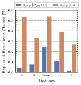
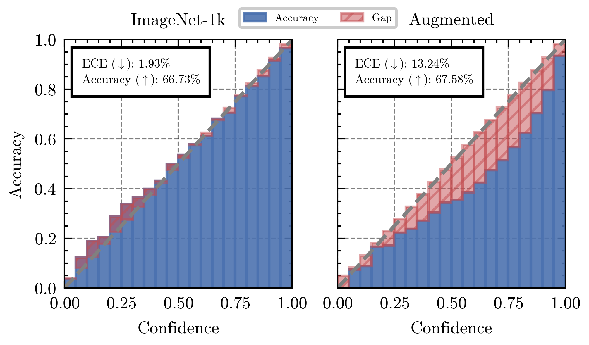
(a) Error of $\overline{p}$ vs $\epsilon(y)$.	(b) Reliability diagrams for IN-1k and its augmented version.

Figure 1: Motivating findings. (a) Comparison between the expected error of CLIP-ViT-B-16, denoted as $\epsilon(y)$, and the error of the marginal probability distribution obtained by marginalizing over examples with the same label, $P_{\hat{y}\neq y}(\overline{p})$; (b) Reliability diagrams of CLIP-ViT-B-16 on the ImageNet validation set (left), and its augmented version (right), showing that augmentations largely un-calibrate CLIP exclusively due to overconfidence while leading to slightly better overall accuracy.

3 Simple and surprisingly strong TTA (for free)

The main point of Section 2.2 is that MEM generally does not affect the predominant class of the marginal probability distribution $\overline{p}$. On the other hand, from Section 2.3 one can conclude that through $\overline{p}$ the model becomes a much stronger classifier. Summarizing:

$$\begin{split}&\text{From Section~{}\ref{sec:entInvariance}: }\operatorname*{arg\,max}\left(\overline{p}(\cdot|\mathbf{x},\bm{\mathbf{t}_{\text{ctx}}})\right)=\operatorname*{arg\,max}\left(\overline{p}(\cdot|\mathbf{x},\bm{\mathbf{t}_{\text{ctx}}}^{*})\right)\\ &\text{From Section~{}\ref{sec:margBound}: }\begin{cases}P_{\hat{y}\neq y}(\overline{p}(\cdot|\mathbf{x},\bm{\mathbf{t}_{\text{ctx}}}))\leq P_{\hat{y}\neq y}(p(\cdot|\mathbf{x},\bm{\mathbf{t}_{\text{ctx}}}))\\ \text{ and, equivalently}\\ P_{\hat{y}\neq y}(\overline{p}(\cdot|\mathbf{x},\bm{\mathbf{t}_{\text{ctx}}}^{*}))\leq P_{\hat{y}\neq y}(p(\cdot|\mathbf{x},\bm{\mathbf{t}_{\text{ctx}}}^{*}))\\ \end{cases}\end{split}$$ (8)

Chaining observations together, it emerges that:

$$\begin{split}P_{\hat{y}\neq y}(p(\cdot|\mathbf{x},\bm{\mathbf{t}_{\text{ctx}}}^{*}))\geq P_{\hat{y}\neq y}(\overline{p}(\cdot|\mathbf{x},\bm{\mathbf{t}_{\text{ctx}}}^{*}))=P_{\hat{y}\neq y}(\overline{p}(\cdot|\mathbf{x},\bm{\mathbf{t}_{\text{ctx}}}))\\ \end{split}$$ (9)

i.e., if all assumptions are met, the error of MEM $\geq$ error of $\overline{p}$ after MEM $=$ error of $\overline{p}$ without MEM. All in all, this TTA framework is hiding a surprisingly strong and optimization-free baseline: $\overline{p}$! Next, we highlight the detrimental impact of data augmentations on this marginal probability distribution and introduce a simple trick to recover its reliability: zeroing-out the Softmax temperature.

3.1 Augmentations undermine the reliability of $\overline{p}$

While augmentations are essential in TTA to obtain multiple views of the test instance, noisy views may constitute Out-of-Distribution (OOD) data, thus having the undesired effect of un-calibrating the model. To sidestep this issue, one can attempt to discriminate between in-distribution (w.r.t. to the pretraining data) and OOD views. Given that low confidence is a common trait in OOD data, a viable way to discriminate is confidence-based filtering, such as in TPT [37]. Formally, a smaller set of confident views are obtained following $X_{filt}=\{\mathbf{x}_{i}\in X|H(p(\cdot|\mathbf{x}_{i},\bm{\mathbf{t}_{\text{ctx}}}))<\rho\}$, where $\rho$ is a threshold retaining the views whose entropy is in the bottom-10% percentile (lowest entropy). Despite its effectiveness, this filter cannot help when the reliability of $\overline{p}$ is undermined by overconfidence.

Augmentations lead to poor calibration. We demonstrate the impact of augmentation-induced overconfidence using the same model and datasets of Section 2.3. For each dataset, we generate an augmented counterpart following the augmentation and filtering setup of TPT [37], i.e.: we augment an input $N=64$ times using simple random resized crops and horizontal flips. Then, we only retain 10% of the $N$ views according to confidence-based filtering, resulting in 6 views per sample. Consequently, each augmented dataset contains $6\times$ more data points than its plain counterpart. The Expected Calibration Error (ECE) [7] reported in Appendix B conveys that ① zero-shot CLIP is well-calibrated (ECE$~{}<0.1$ for all datasets), strongly supporting the theory of Section 2.3 and ② the augmented visual space greatly increases the calibration error.

Poor calibration is always caused by overconfidence. We investigate the reason for the increase in ECE by presenting reliability diagrams for the ImageNet validation set in Fig. 1(b). In a reliability diagram, every bar below the identity line $y=x$ signals overconfidence (i.e., the confidence on the x-axis prevails over the accuracy on the y-axis), while the opposite signals under-confidence. Notably, the ECE increases exclusively due to overconfidence. The error rate, in contrast, decreases slightly. As displayed in Appendix B, this phenomenon persists across all datasets.

3.2 Zero: Test-Time Adaptation with “zero” temperature

Since its reliability is severely undermined by augmentations-induced overconfidence, directly predicting through $\overline{p}$ is not an enticing baseline for TTA. Concurrently, we also know that the error rate does not decrease when predicting over the augmented visual space. Hence, we are interested in finding an efficient way to capitalize on these observations: relying on the predictions over the views, while ignoring potentially misleading confidence information. The key is to note that both desiderata are obtained by explicitly tweaking a single parameter of the model: the temperature. Specifically, setting the temperature to (the limit of) zero corresponds to converting probability distributions into one-hot encodings, hence exclusively relying on their $\operatorname*{arg\,max}$ when marginalizing. Inspired by this idea we propose Zero, Test-Time Adaptation with “zero” temperature.

Procedure. Zero follows these simple steps: ① augment, ② predict, ③ retain the most confident predictions, ④ set the Softmax temperature to zero and ⑤ marginalize. The final prediction is the $\operatorname*{arg\,max}$ of the marginal probability distribution computed after “zeroing-out” the temperature, i.e.:

$$\textsc{Zero}(\mathbf{x},\bm{\mathbf{t}_{\text{ctx}}},C)=\operatorname*{arg\,max}_{c\in[1,\ldots,C]}\left(\sum_{i=1}^{N}\mathbbm{1}(\mathbf{x}_{i}\in X_{filt})\lim_{\tau\to 0^{+}}{p}(y=c|\mathbf{x}_{i},\bm{\mathbf{t}_{\text{ctx}}},\tau)\right),$$ (10)

where $\mathbbm{1}$ is an indicator function, whose output is $1$ if $\mathbf{x}_{i}\in X_{filt}$ and $0$ otherwise, and $X_{filt}$ is the set of confident views before tweaking the temperature, i.e., $\mathbf{x}_{i}\in X_{filt}$ if $H(p(\cdot|\mathbf{x}_{i},\bm{\mathbf{t}_{\text{ctx}}},\tau)<\rho$.

Algorithm 1 PyTorch-style code for Zero

⬇

# z_txt = pre-computed text embeddings (C,hdim)

# temp = model’s original temp

# augment = takes (C,H,W) and returns (N,C,H,W)

# gamma = filtering percentile (e.g., 0.1)

def zero(image, z_txt, N, gamma, temp):

# step1: augment

views = augment(image, num_views=N)

# step2: predict (unscaled logits)

l = model.image_encoder(views) @ z_txt.t()

# step3: retain most confident preds

l_filt = confidence_filter(l, temp, top=gamma)

# step4: zero temperature

zero_temp = torch.finfo(l_filt.dtype).eps

# step5: marginalize

p_bar = (l_filt / zero_temp).softmax(1).sum(0)

return p_bar.argmax()

Efficient Implementation. In all its simplicity, Zero is computationally lightweight. In closed set assumptions where the class descriptions (and thus their embeddings) are fixed, Zero only requires a single batched forward pass through the vision encoder, just as much as needed to forward the $N$ views. Additionally, since the temperature is explicitly tweaked, Zero needs no backpropagation at all and can be implemented in a few lines of code. For reference, a PyTorch-like implementation [29] is reported in Algorithm 1.

Equivalent perspective and final remark. We bring to attention a simple scheme which corresponds to Zero: voting over (confident) augmentations. Drawing from the theory of ensembling, note that the error rate of the voting paradigm is exactly described by Eq. (6). Essentially, this means that Zero capitalizes on the theoretical insights while circumventing practical issues stemming from augmentations. We also highlight that Zero is subtly hidden within any TTA framework relying exclusively on MEM, since computing $\overline{p}$ is inevitable therein. For this reason, we refer to Zero as a baseline for TTA. Our goal diverges from introducing a “novel” state-of-the-art method for TTA. In contrast, we advocate the importance of evaluating simple baselines.

4 Experiments

Table 1: Natural Distribution Shifts. TTA methods are grouped according to the baseline model and top-1 accuracy is reported. Bold text is the best method within each group.

Method	ImageNet	A	V2	R	Sketch	Average
CLIP-ViT-B-16
Zero-Shot	66.73	47.87	60.86	73.98	46.09	59.11
Ensemble	68.34	49.89	61.88	77.65	48.24	61.20
TPT	68.98	54.77	63.45	77.06	47.94	62.44
Zero	69.06$\pm$0.04	61.35$\pm$0.26	64.13$\pm$0.17	77.28$\pm$0.08	48.29$\pm$0.04	64.02
Zero+Ensemble	70.93$\pm$0.02	64.06$\pm$0.09	65.16$\pm$0.21	80.75$\pm$0.08	50.32$\pm$0.09	66.24
MaPLe
Zero-Shot	-	50.90	64.07	76.98	49.15	60.28
TPT	-	58.08	64.87	78.12	48.16	62.31
PromptAlign	-	59.37	65.29	79.33	50.23	63.55
Zero	-	64.65$\pm$0.24	66.63$\pm$0.32	79.75$\pm$0.41	50.73$\pm$0.62	65.44
CLIP-ViT-B-16 + CLIP-ViT-L-14
ZeroShot	73.44	68.82	67.80	85.40	57.84	70.66
RLCF ${}_{t=3}^{\bm{\mathbf{t}_{\text{ctx}}}}$	73.23	65.45	69.77	83.35	54.74	69.31
RLCF ${}_{t=3}^{\Theta_{v}}$	74.85	73.71	69.77	86.19	57.10	72.32
Zero	74.48$\pm$0.12	77.07$\pm$0.35	69.53$\pm$0.12	86.87$\pm$0.05	58.59$\pm$0.08	73.31

In this section, we present a comprehensive experimental evaluation of Zero. Our results show that Zero, alongside its simplicity, is an effective and efficient approach for TTA.

4.1 Experimental Protocol

Baselines. We compare Zero to three strategies for TTA with VLMs: ① TPT [37], ② PromptAlign [32], and ③ Reinforcement Learning from CLIP Feedback (RLCF) [53]. As introduced in Section 2, TPT works by minimizing the entropy of $\overline{p}$. In contrast, PromptAlign relies on a pretrained MaPLe initialization [14] and pairs the MEM objective with a distribution alignment loss between layer-wise statistics encountered online and pretraining statistics computed offline. Finally, RLCF does not include MEM in its framework; Zhao et al. [53] shows that, if rewarded with feedback from a stronger teacher such as CLIP-ViT-L-14, the smaller CLIP-ViT-B-16 can surpass the teacher itself.

Models. As different approaches consider different backbones in the original papers, we construct different comparison groups to ensure fair comparisons with all TTA baselines [37, 32, 53].

Group 1: When comparing to TPT, we always use CLIP-ViT-B-16. Shu et al. [37] also reports CLIP-Ensemble, i.e., CLIP enriched with an ensemble of hand-crafted prompts. While the design of TPT does not allow leveraging text ensembles (as also pointed out by concurrent work [41]), Zero seamlessly integrates with CLIP-Ensemble. We denote this variant with Zero_+Ensemble.

Group 2: When comparing to PromptAlign, we follow Samadh et al. [32] and start from a MaPLe initialization for a fair comparison. Within this group, we also report TPT on top of MaPLe, as in [32].

Group 3: When comparing to RLCF, we use both CLIP-ViT-B-16 and CLIP-ViT-L-14 as in [53]. Specifically, confidence-based filtering acts on top of the output of the first model, and the selected inputs are passed to the second model for the final output. Both forward passes are inevitable in RLCF, so this scheme corresponds to “early-exiting” the pipeline, exactly as per MEM. RLCF can vary according to (i) the parameter group being optimized and (ii) the number of adaptation steps. We denote with $\Theta_{v}$ the full image encoder tuning, with $\bm{\mathbf{t}_{\text{ctx}}}$ prompt tuning, and with $t$ the number of adaptation steps. For example, RLCF ${}_{t=3}^{\bm{\mathbf{t}_{\text{ctx}}}}$ indicates RLCF with prompt tuning for 3 TTA steps.

Benchmarks. We follow the established experimental setup of [37, 32], evaluating Zero on Natural Distribution Shifts and Fine-grained Classification. For the former, we consider the ImageNet validation set and the four datasets for Natural Distribution Shifts already presented in Section 2, commonly considered Out-of-Distribution (OOD) datasets for CLIP. For fine-grained classification, we evaluate all TTA methods on 9 datasets. Specifically, we experiment with Oxford-Flowers (FWLR) [24], Describable Textures (DTD) [2], Oxford-Pets (PETS) [28], Stanford Cars (CARS) [16], UCF101 (UCF) [40], Caltech101 (CAL)[5], Food101 (FOOD) [1], SUN397 (SUN)[47], and FGVC-Aircraft (AIR) [22]. For these, we refer to the test split in Zhou et al. [55] as per the common evaluation protocol. Unless otherwise specified, all tables in this section report top-1 accuracy.

Implementation Details. $\mathcal{A}$ only contains random resized crops and random horizontal flips. We do not tune any hyperparameter; instead, we inherit the setup of TPT with $N=64$ and the top percentile for confidence-based filtering set to $0.1$. To ensure hardware differences do not play any role in comparisons, we execute all TTA methods under the same hardware setup by running the source code of each repository with no modifications. We always use 1 NVIDIA A100 GPU and FP16 Automatic Mixed Precision. Results are averaged over 3 different seeds.

Table 2: Finegrained classification. TTA methods are grouped according to the reference baseline, top-1 accuracy is reported and bold text indicates the best performer of each group.

Method	FLWR	DTD	PETS	CARS	UCF	CAL	FOOD	SUN	AIR	Avg
CLIP-ViT-B-16
Zero-Shot	67.44	44.27	88.25	65.48	65.13	93.35	83.65	62.59	23.67	65.98
Ensemble	67.07	45.09	88.28	66.16	67.51	93.91	84.04	66.26	23.22	66.84
TPT	68.75	47.04	87.23	66.68	68.16	93.93	84.67	65.39	23.13	67.22
Zero	67.07	45.80	86.74	67.54	67.64	93.51	84.36	64.49	24.40	66.84
Zero+Ensemble	66.82	45.86	87.20	68.48	68.57	94.14	84.58	66.90	24.42	67.44
MaPLe
Zero-Shot	72.23	46.49	90.49	65.57	68.69	93.53	86.20	67.01	24.74	68.33
TPT	72.37	45.87	90.72	66.50	69.19	93.59	86.64	67.54	24.70	68.57
PromptAlign	72.39	47.24	90.76	68.50	69.47	94.01	86.65	67.54	24.80	69.04
Zero	71.20	47.70	90.17	67.91	69.49	94.12	86.78	67.55	25.57	68.94
CLIP-ViT-B-16 + CLIP-ViT-L-14
ZeroShot	75.76	51.83	92.86	76.16	73.70	94.04	88.03	66.96	30.54	72.21
RLCF ${}_{t=1}^{\bm{\mathbf{t}_{\text{ctx}}}}$	71.58	50.34	89.01	69.76	69.84	94.09	85.90	67.33	23.71	69.06
RLCF ${}_{t=3}^{\bm{\mathbf{t}_{\text{ctx}}}}$	72.49	51.93	89.55	72.91	72.31	95.00	86.84	69.04	25.40	70.61
RLCF ${}_{t=1}^{\Theta_{v}}$	72.56	52.21	89.51	63.12	71.49	94.65	86.90	68.50	24.06	69.22
RLCF ${}_{t=3}^{\Theta_{v}}$	71.74	53.27	91.15	70.93	73.24	94.73	87.28	69.38	28.54	71.14
Zero	75.34	54.22	92.90	77.33	74.26	94.52	87.57	68.05	32.11	72.92

4.2 Results

Natural Distribution Shifts. Results for Natural Distribution Shifts are reported in Table 1.

Group 1 (TPT): Zero surpasses TPT consistently on all datasets. Among OOD datasets, peak difference is reached with ImageNet-A, where Zero outperforms TPT by $+6.58\%$. Enriching Zero with hand-crafted prompts improves results further, with an average margin of $+3.80\%$ w.r.t. TPT.

Group 2 (PromptAlign): Within the second comparison group, Zero outperforms PromptAlign on all datasets, with $+1.89\%$ being the gap in average performance. Note also that Zero consistently outperforms TPT also when the baseline initialization is MaPLe (by an average of $+3.13\%$).

Group 3 (RLCF): We follow [53] and report RLCF variants with $t=3$ steps. In this group, Zero outperforms RLCF in 3 out of 5 datasets, with a gap in the average performance of $+0.99\%$. Importantly, RLCF is only close to Zero with image encoder tuning; only prompt tuning is insufficient.

Fine-grained Classification. Results for fine-grained classification are shown in Table 2. To foster readability, the standard deviations of Zero are separately reported in Table 6 (Appendix).

Group 1 (TPT): Default Zero improves over the zero-shot baseline CLIP-ViT-B-16, but is slightly outperformed by TPT with an average margin of $-0.38\%$. However, extending Zero with hand-crafted prompts (something that TPT cannot do by design) is sufficient to outperform TPT on 5 out of 9 datasets, and obtain an average improvement of $+0.22\%$.

Group 2 (PromptAlign): On average, PromptAlign has a slight improvement of $+0.1\%$ over Zero. However, note that this is mostly influenced by the performance on one dataset only (Oxford-Flowers) and that, in contrast, Zero surpasses PromptAlign in 6 out of 9 datasets. In line with the previous benchmark, Zero better adapts MaPLe than TPT, outperforming it in 7 out of 9 datasets.

Group 3 (RLCF): As Zhao et al. [53] do not report results on fine-grained classification, we use their code to evaluate four RLCF variants: $\Theta_{v}$ and $\bm{\mathbf{t}_{\text{ctx}}}$ tuning, with $t=1$ and $t=3$ adaptation steps. We find that Zero largely outperforms RLCF regardless of the configuration. Even with respect to the strongest RLCF ${}_{t=3}^{\Theta_{v}}$ variant, Zero obtains an average improvement of $+1.78\%$.

Computational Requirements. The complexity of Zero does not scale linearly with the size of the label space, as it does for prompt-tuning strategies. To quantify the computational gain of Zero w.r.t. other TTA methods, we report the runtime per image and peak GPU memory in Table 3 under the same hardware requirements (1 NVIDIA RTX 4090). We compare to TPT and the RLCF pipeline in a worst-case scenario where the label space is large (ImageNet). We omit PromptAlign from our analysis since it has slightly worse computational performance than TPT.

Zero is $9.5\times$ faster than TPT taking $12.61\times$ less memory, corresponding to an order of magnitude of computational savings in both time and space.

Table 3: Computational requirements of different TTA methods.

Metric	CLIP-ViT-B-16		CLIP-ViT-B-16 + CLIP-ViT-L-14
	TPT	Zero	RLCF ${}_{t=3}^{\bm{\mathbf{t}_{\text{ctx}}}}$	RLCF ${}_{t=3}^{\Theta_{v}}$	Zero
Time [$s$]	0.57$\pm 0.01$	0.06$\pm 0.01$	1.20$\pm 0.02$	0.18$\pm 0.01$	0.08$\pm 0.02$
Mem [GB]	17.66	1.40	18.64	9.04	2.58

Concerning the slowest RLCF variant (prompt tuning), Zero is $15\times$ faster and takes $7.22\times$ less memory. In the faster RLCF ${}^{\Theta_{v}}$, text classifiers are also cached; nevertheless, Zero is $2.25\times$ faster and $3.5\times$ more memory friendly.

5 Related Work

Closest to our work is a recent and very active research thread focusing on Episodic TTA with VLMs [37, 32, 53, 41]. As discussed in the manuscript, these methods mostly rely on prompt learning, a parameter-efficient strategy that only trains over a small set of input context vectors [19]. Narrowing down to VLMs, notable examples of prompt learning approaches include CoOp [55], CoCoOp [54], and MaPLe [14]. Episodic TTA has also been explored with traditional unimodal networks, such as ResNets [9], where MEM is still a core component [52]. In this context, MEM has recently been enriched with sharpness- [26] or shape-aware filtering [18]. Due to its nature, Episodic TTA is completely agnostic to the temporal dimension and is powerful when no reliable assumptions on the test data can be taken. Some other works relax these constraints and integrate additional assumptions such as batches of test data being available instead of single test points [44]. When test data are assumed to belong to the same domain, one can rely on various forms of knowledge retention as a powerful mechanism to gradually incorporate domain knowledge [20, 21] or avoid forgetting [25]. The synergy between TTA and retrieval is also emerging as a powerful paradigm when provided with access to huge external databases [8, 49]. We particularly believe this can be a promising direction.

Closely related to our work are also Test-Time Training (TTT) and TTAug. In TTT the same one sample learning problem of Episodic TTA is tackled with auxiliary visual self-supervised tasks, such as rotation prediction [42] or masked image modeling [6], which require specialized architecture heads and are not directly applicable to VLMs. TTAug has recently been theoretically studied [15]. It boils down to producing a large pool of augmentations to exploit at test time [34], or to learn from [43]. In all its simplicity, Zero can be seen as a strong TTAug baseline for VLMs, which, differently from concurrent work [50], does not involve any form of optimization.

6 Limitations

Zero can seamlessly adapt a wide range of VLMs on arbitrary datasets without requiring extensive computational resources and is backed by theoretical justifications. However, we delineate three major limitations to our method which we report here. The first limitation concerns the preliminary observations which led to Zero, such as augmentation-induced overconfidence. For example, these observations may not persist if the VLM changes significantly in the future, potentially leading to poor adaptation. The second limitation stems from theoretical assumptions, the core one being the invariance of the marginal probability distribution to marginal entropy minimization. While our proposition guarantees invariance if entropy is minimized and the negative delta to the probability of the prevailing class is inferior to its default value, these theoretical assumptions may not hold all the times. In this work, we supported our assumptions with empirical verification but, as per the first limitation, these may not extend to the space of all models and datasets (as we have shown, for example, with satellite imagery). A third worthy-of-note limitation relates to the independence assumption among the views from which the marginal probability distribution is obtained. As we discussed in Section 2.3, the views themselves do not have any direct dependency, but they are still partially related through the source image from which they stem. Related to this, we particularly believe that extending Zero in a Retrieval-Augmented TTA setup can largely mitigate this limitation. Finally, despite being much lighter than the current state-of-the-art TTA strategies, Zero’s computational requirements in the visual branch scale linearly with the number of views, since all of them need to be independently forwarded. On this, we believe that exploring how to augment directly in the latent visual space to also circumvent the forward pass of the vision encoder is an intriguing direction.

7 Conclusions

We theoretically investigated Marginal Entropy Minimization, the core paradigm of the current research in Test-Time Adaptation with VLMs. Building on our theoretical insights, we introduced Zero: a frustratingly simple yet strong baseline for TTA, which only relies on a single batched forward pass of the vision encoder. Our experimental results on Natural Distribution Shifts and Fine-grained Classification unveil that Zero favorably compares to state-of-the-art TTA methods while requiring relatively negligible computation. We hope our findings will inspire researchers to push the boundaries of TTA further.

Appendix A Marginal Entropy Minimization does not influence $\operatorname*{arg\,max}\overline{p}$

A.1 Proof of Proposition 2.1.

Proof.

Let us denote the pre-TTA $p^{\text{init}}(c)=\overline{p}(y=c|\mathbf{x},\bm{\mathbf{t}_{\text{ctx}}})$ and the post-TTA $p^{\text{end}}(c)=\overline{p}(y=c|\mathbf{x},\bm{\mathbf{t}_{\text{ctx}}}^{*})$, i.e., the marginal probabilities before and after optimizing $\bm{\mathbf{t}_{\text{ctx}}}$. Let $c^{\text{init}}$ and $c^{\text{end}}$ denote the predictions before and after TTA, i.e., $c^{\text{init}}=\operatorname*{arg\,max}p^{\text{init}}$ and $c^{\text{end}}=\operatorname*{arg\,max}p^{\text{end}}$.

To simplify the notation, let us use $\mathbf{z}^{*\text{txt}}$ to write any post-TTA text embedding $\mathbf{z}^{\text{txt}}(\bm{\mathbf{t}_{\text{ctx}}}^{*})$.

Under the assumption that entropy is minimized (the optimal scenario for MEM), we have $p^{\text{end}}(c^{\text{end}})=1$, and $p^{\text{end}}(c)=0~{}\forall~{}c\neq c^{\text{end}}$.

Let us rewrite the final distribution $p^{\text{end}}$ using the function $g$ introduced in Sec.2.2. Specifically, for any class $c$, we have:

$$p^{\text{end}}(c)=\frac{1}{N}\sum_{i}^{N}\frac{\exp\left(\mathbf{z}^{\text{img}}_{i}\cdot\mathbf{z}_{c}^{\text{txt}}(\bm{\mathbf{t}_{\text{ctx}}}^{*})/\tau\right)}{\sum_{k}^{C}\exp\left(\mathbf{z}^{\text{img}}_{i}\cdot\mathbf{z}_{k}^{\text{txt}}(\bm{\mathbf{t}_{\text{ctx}}}^{*})/\tau\right)}=\frac{1}{N}\sum_{i}g(c,\mathbf{z}^{\text{img}}_{i},\mathbf{z}_{1}^{*\text{txt}},\ldots,\mathbf{z}_{C}^{*\text{txt}}).$$ (11)

Performing a first-order Taylor expansion on $g$, we have:

$$\begin{split}&g(c,\mathbf{z}^{\text{img}}_{i},\mathbf{z}_{1}^{*\text{txt}},\ldots,\mathbf{z}_{C}^{*\text{txt}})=g(c,\mathbf{z}^{\text{img}}_{i},\mathbf{z}_{1}^{\text{txt}},\ldots,\mathbf{z}_{C}^{\text{txt}})+\\ &(\nabla_{[\mathbf{z}_{1}^{\text{txt}},\ldots,\mathbf{z}_{C}^{\text{txt}}]}g)^{t}([\mathbf{z}_{1}^{*\text{txt}},\ldots,\mathbf{z}_{C}^{*\text{txt}}]-[\mathbf{z}_{1}^{\text{txt}},\ldots,\mathbf{z}_{C}^{\text{txt}}]).\end{split}$$ (12)

We can also write any post-TTA text embedding $\mathbf{z}_{c}^{\text{txt}}(\bm{\mathbf{t}_{\text{ctx}}}^{*})$ as a function of the text encoder $\mathbf{E}_{\text{txt}}$ prompted with optimized context vectors:

$$\begin{split}\mathbf{z}_{c}^{\text{txt}}(\bm{\mathbf{t}_{\text{ctx}}}^{*})=\mathbf{E}_{\text{txt}}([\bm{\mathbf{t}_{\text{ctx}}}^{*},\mathbf{t}_{c}])=\mathbf{E}_{\text{txt}}([\bm{\mathbf{t}_{\text{ctx}}}-\lambda\nabla_{\bm{\mathbf{t}_{\text{ctx}}}}H,\mathbf{t}_{c}]).\end{split}$$ (13)

Through another first-order Taylor expansion (this time on $\mathbf{z}_{c}^{\text{txt}}(\bm{\mathbf{t}_{\text{ctx}}}^{*})$), we have:

$$\begin{split}&\mathbf{z}_{c}^{\text{txt}}(\bm{\mathbf{t}_{\text{ctx}}}^{*})=\mathbf{E}_{\text{txt}}([\bm{\mathbf{t}_{\text{ctx}}},\mathbf{t}_{c}])+(\nabla_{\bm{\mathbf{t}_{\text{ctx}}}}\mathbf{E}_{\text{txt}})^{t}(\mathbf{z}_{c}^{\text{txt}}(\bm{\mathbf{t}_{\text{ctx}}}^{*})-\mathbf{z}_{c}^{\text{txt}}(\bm{\mathbf{t}_{\text{ctx}}}))=\\ &\mathbf{E}_{\text{txt}}([\bm{\mathbf{t}_{\text{ctx}}},\mathbf{t}_{c}])-\lambda(\nabla_{\bm{\mathbf{t}_{\text{ctx}}}}\mathbf{E}_{\text{txt}})^{t}\nabla_{\bm{\mathbf{t}_{\text{ctx}}}}(H),\end{split}$$ (14)

leading to an equivalent re-writing:

$$\mathbf{z}_{c}^{\text{txt}}(\bm{\mathbf{t}_{\text{ctx}}}^{*})=\mathbf{z}_{c}^{\text{txt}}(\bm{\mathbf{t}_{\text{ctx}}})-\lambda(\nabla_{\bm{\mathbf{t}_{\text{ctx}}}}\mathbf{E}_{\text{txt}})^{t}\nabla_{\bm{\mathbf{t}_{\text{ctx}}}}(H)$$ (15)

Substituting (15) into (12), we can express $g$ as follows:

$$\begin{split}&g(c,\mathbf{z}^{\text{img}}_{i},\mathbf{z}_{1}^{*\text{txt}},\ldots,\mathbf{z}_{C}^{*\text{txt}})=g(c,\mathbf{z}^{\text{img}}_{i},\mathbf{z}_{1}^{\text{txt}},\ldots,\mathbf{z}_{C}^{\text{txt}})-\lambda(\nabla_{[\mathbf{z}_{1}^{\text{txt}},\ldots,\mathbf{z}_{C}^{\text{txt}}]}g)^{t}\mathbf{d}\\ &\text{where }\mathbf{d}\in\mathbb{R}^{C}\text{s.t.}~{}\mathbf{d}_{k}=(\nabla_{\bm{\mathbf{t}_{\text{ctx}}}}\mathbf{E}_{\text{txt}}([\bm{\mathbf{t}_{\text{ctx}}},\mathbf{t}_{k}]))^{t}\nabla_{\bm{\mathbf{t}_{\text{ctx}}}}(H)([\bm{\mathbf{t}_{\text{ctx}}},\mathbf{t}_{k}]))~{}~{}\forall k\in\{1,\ldots,C\},\end{split}$$ (16)

with $\mathbf{d}_{k}$ denoting the $k$-th entry of the $C$ dimensional vector $\mathbf{d}$. From (12) and (16) the negative variation $\delta g(c,\mathbf{z}^{\text{img}})$ to $g$ before and after MEM can be expressed as:

$$\begin{split}&\delta g(c,\mathbf{z}^{\text{img}})=\lambda(\nabla_{[\mathbf{z}_{1}^{\text{txt}},\ldots,\mathbf{z}_{C}^{\text{txt}}]}g)^{t}\mathbf{d}\end{split}$$ (17)

Finally, for any class, we can rewrite its final probability $p^{\text{end}}$ as a function of its initial probability $p^{\text{init}}$ and the variation of $g$ before and after TTA for the same class:

$$p^{\text{end}}(c)=p^{\text{init}}(c)-\frac{\lambda}{N}\sum_{i}\delta g(c,\mathbf{z}_{i}^{\text{img}})$$ (18)

From Eq.(18) we have that if $p^{\text{init}}(c^{\text{init}})>\frac{\lambda}{N}\sum_{i}\delta g(c^{\text{init}},\mathbf{z}_{i}^{\text{img}})$, then the final probability $p^{\text{end}}(c^{\text{init}})>0$. In the optimal case for MEM the entropy of $p^{\text{end}}$ is minimized, which entails that only one class can have a probability strictly greater than 0. Hence, $c^{\text{init}}=c^{\text{end}}$.

∎

A.2 Experimental verification

Table 4: Empirical evidence supporting Proposition 2.1.

Proposition	IN-1k	IN-A	IN-v2	IN-R	IN-Sketch
$\operatorname*{arg\,max}p^{\text{init}}=\operatorname*{arg\,max}p^{\text{end}}~{}[\%]$	95.73$\pm 0.05$	95.55$\pm 0.12$	94.86$\pm 0.17$	96.78$\pm 0.08$	91.23$\pm 0.09$

We support the previous proposition with empirical evidence, by manually counting how often the prediction of $\overline{p}$ is invariant to Test-Time Prompt Tuning by MEM. This experiment is easy to reproduce and consists of the following: augment $N$ times, filter by confidence, compute $p^{\text{init}}$, optimize by MEM, compute $p^{\text{end}}$ and check if $\operatorname*{arg\,max}p^{\text{init}}=\operatorname*{arg\,max}p^{\text{end}}$. We report the proportion of samples for which the proposition holds for all Natural Distribution Shifts datasets in Table 4, averaged over 3 runs with different seeds (the same used in Sec. 4 of the main body). Although the proposition only accounts for the cases where entropy is globally minimized, the table shows that the marginal probability distribution is largely invariant to MEM. In the best case (ImageNet-Sketch) MEM alters the prediction of $\overline{p}$ only $8.77\%$ of the times. In the worst case (ImageNet-R), the prediction is unaltered for $96.78\%$ samples.

Appendix B Calibration and Overconfidence of CLIP on augmented Natural Distribution Shifts

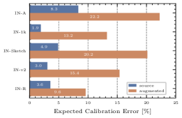
Figure 2: Expected Calibration Error (ECE) [7] of CLIP-ViT-B-16 across 5 datasets for robustness to natural distribution shifts. Blue is the ECE of zero-shot CLIP, orange is the ECE of zero-shot CLIP on an augmented version of the dataset after confidence-based thresholding.

In Section 3.1 of the manuscript, the validation set of ImageNet-1k is shown to convey that overconfidence emerges as a critical issue when predicting over augmented views. In this appendix, we expand the analysis to the 4 datasets for robustness to Natural Distribution Shifts (NDS) [12, 11, 31, 45]. For all datasets, we follow the augmentation setup of Sec.3.1, and generate augmented counterparts with $6\times$ more examples.

First, let us define the calibration of DNNs. Calibrating DNNs is crucial for developing reliable and robust AI systems, especially in safety-critical applications. A DNN is perfectly calibrated if the probability that its prediction is correct ($\hat{y}=y$) given a confidence score random variable $S$ is equal to its confidence score, which in our case is $s=\max\overline{p}(\cdot)$:

$$P(\hat{y}=y|S=s)=s$$ (19)

To evaluate the expected calibration error (ECE), we typically split the dataset into $M$ bins $B_{m}$ based on their confidence scores. We then calculate the accuracy of each bin, denoted as $\text{acc}(B_{m})$, and the average confidence, denoted as $\text{conf}(B_{m})$. The ECE is defined by the following formula:

$$\text{ECE}=\frac{1}{M}\sum_{m}^{M}\|\text{acc}(B_{m})-\text{conf}(B_{m})\|$$ (20)

Then, we show how the ECE of CLIP-ViT-B-16 varies between “source” and augmented versions of all datasets (ImageNet-1k included) in Figure 2. From this experiment, we observe a large increase in the ECE across all datasets. In no cases, the ECE remains comparable to its default value when no augmentations are present. As we discussed in 3.1, the calibration error increases when the model is either more accurate than confident (signaling underconfidence) or the opposite, signaling overconfidence. Reliability diagrams are a standard tool to understand which is the case, hence we show them for all 4 NDS Datasets in Fig.3.

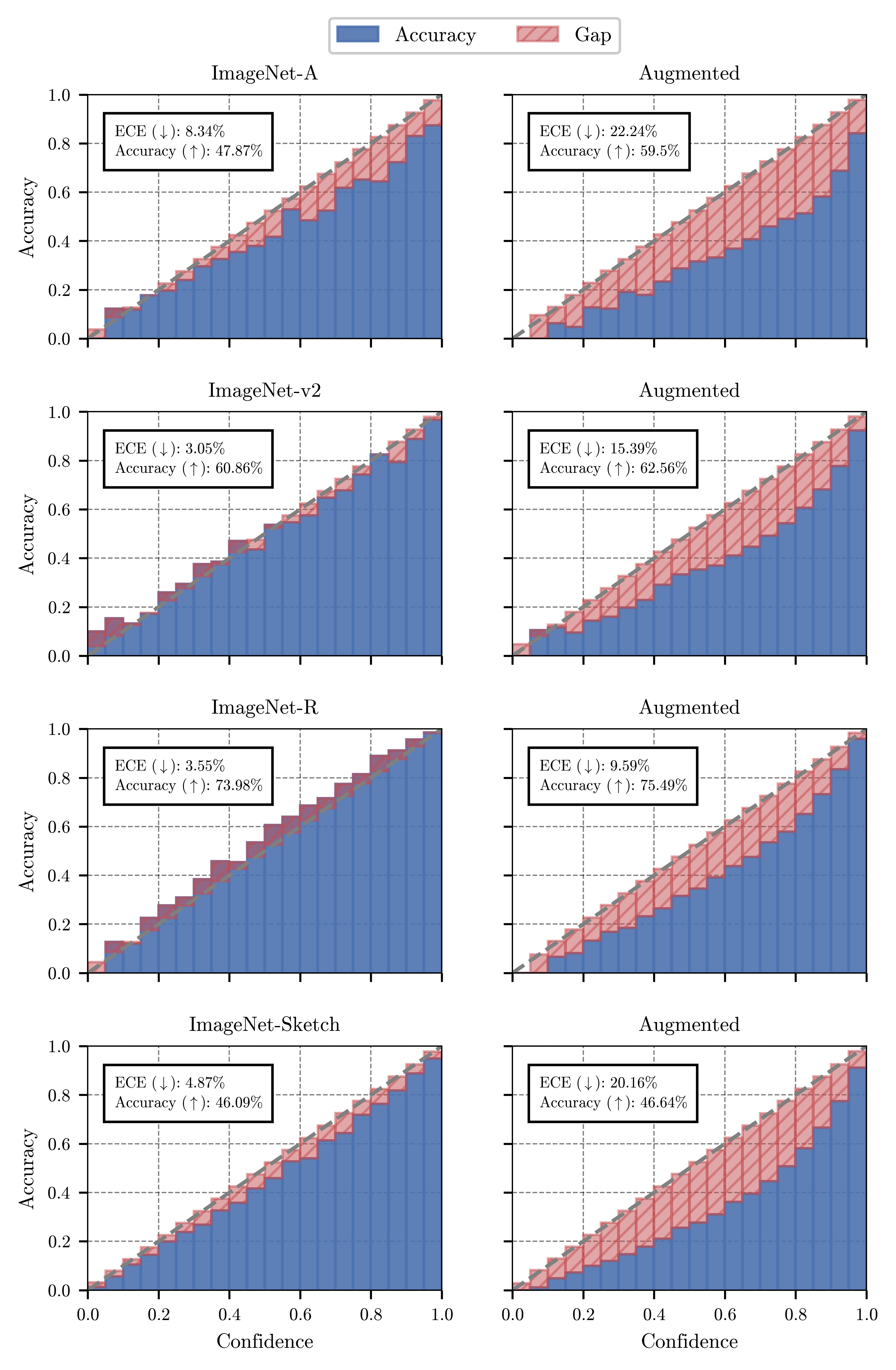
Figure 3: Reliability diagrams (20 bins) for CLIP-ViT-B-16 on the 4 datasets for Natural Distribution Shifts. In each row, left is the ECE on the source dataset, right on the augmented and filtered version. Row 1: ImageNet-A [12]; Row 2: ImageNet-v2 [31]; Row 3: ImageNet-R [11]; Row 4: ImageNet-Sketch [45].

These results are entirely consistent with Sec.3.1: the calibration error increases exclusively due to overconfidence, no matter the dataset. In parallel, the error rate of CLIP-ViT-B-16 can either remain close to its default value (e.g., ImageNet-Sketch), slightly decrease (e.g., ImageNet-R and -v2) or largely decrease (ImageNet-A).

Appendix C On the expected risk of $\overline{p}$ and $p$.

The expected risk of a classifier $f$ is commonly defined as the expectation of the risk function $\ell$ over the joint distribution of data and labels.

$$\mathcal{R}(f)=\mathbb{E}_{(x,y)\sim P_{\mathcal{X}\mathcal{Y}}}\Big{[}\ell(y,f(\mathbf{x}))\Big{]}.$$ (21)

In [15], the expected risk of a classifier $\overline{f}(\mathbf{x})=\overline{p}(\cdot|\mathbf{x})$, which predicts by marginalizing over several augmented views, is theoretically shown to lower-bound the empirical risk of a standard classifier $f=p(\cdot|\mathbf{x})$ when the risk function $\ell$ is a squared error, i.e., $\ell(a,b)=(a-b)^{2}$.

Here, we show that such a bound can be extended to any risk function $\ell$ that checks the triangular inequality. Specifically, note that if $\ell$ satisfies the triangular inequality, then:

$$\ell(y,\overline{p}(\mathbf{x}))\leq\frac{1}{N}\sum_{i=1}^{N}\ell(y,p(\mathbf{x}_{i})).$$ (22)

The above inequality is obtained following these simple steps:

$$\|y-\overline{p}(\mathbf{x})\|=\|y-\frac{1}{N}\sum_{i=1}^{N}p(\mathbf{x}_{i})\|=\|\frac{1}{N}\sum_{i=1}^{N}(y-p(\mathbf{x}_{i}))\|\leq\frac{1}{N}\sum_{i=1}^{N}\|(y-p(\mathbf{x}_{i}))\|$$ (23)

Applying the expectation operator $\mathbb{E}$ over the joint distribution ${P}_{\mathcal{X}\mathcal{Y}}$ to both sides of Eq.(22) leads to:

$$\mathcal{R}(\overline{p})\leq\frac{1}{N}\sum_{i=1}^{N}\mathcal{R}(p)=\mathcal{R}(p).$$ (24)

Hence, the empirical risk of $\overline{p}$ lower-bounds that of $p$ for any risk function $\ell$ satisfying the triangular inequality.

Appendix D Tie breaking with Zero

A caveat of Zero are ties, i.e., cases with multiple classes having identical probability within the marginal probability distribution. This is clear to see when viewing Zero as its equivalent paradigm of voting among confident views, simply because more than one class may have an equal amount of “votes”. Throughout all the experiments of this work, ties are broken greedily. If a tie results from the top-10% views, the procedure for breaking it follows these two steps: ① sort the remaining 90% views by ascending entropy (most to least confident) and ② scan the views until a prediction is encountered that breaks the tie. Other than this, many alternative are possible, such as relying on the most confident prediction. Specifically, we have explored the following alternatives:

1. greedy tie breaking, as discussed above;

2. relying on the most confident prediction;

3. computing several marginal probabilities for $\overline{p}$, each by marginalizing over views with identical predictions, and picking the one with the lowest entropy for the final decision;

4. relying on the maximum logit (pre-Softmax);

5. using the averaged logits (pre-Softmax);

6. doing similar to point 2, using logits instead of probabilities;

7. random tie breaking;

and did not find consistent behaviour across all (fine-grained and NDS) datasets, suggesting this is indeed a minor component. We opted for greedy tie breaking due to its slightly better performance on the ImageNet validation set.

Appendix E A failure mode for TTA: satellite imagery

In our experiments, we find that an extremely OOD domain represent a consistent failure mode for TTA: satellite imagery. In all comparison groups, a zero-shot baseline largely outperforms any TTA strategy: in Group 1 the zero-shot baseline CLIP-Ensemble largely outperforms the best TTA strategy Zero_+Ensemble ($50.42\%$ vs $43.77\%$); in Group 2, zero-shot MaPLe outperforms PromptAlign ($48.06\%$ vs $47.86\%$) and in Group 3 the best RLCF${}_{t=1}^{\Theta_{v}}$ pipeline lies far behind the zero-shot teacher CLIP-ViT-L-14 ($47.74\%$ vs $54.38\%$) when evaluated on EuroSat[10]. For completeness, results for all groups are reported in Tab.5. Here, we qualitatively and quantitatively report two main root causes for failures.

Table 5: TTA failures on EuroSAT.

Model	Method	Top1-Acc [$\%$]
CLIP-ViT-B-16	Zero-Shot	42.01
	Ensemble	50.42
	TPT	42.86
	Zero	39.60
	Zero+Ensemble	43.77
MaPLE	Zero-Shot	48.06
	TPT	47.80
	PromptAlign	47.86
	Zero	41.05
CLIP-ViT-B-16 + CLIP-ViT-L-14	Zero-Shot	54.38
	RLCF${}_{t=1}^{\bm{\mathbf{t}_{\text{ctx}}}}$	46.87
	RLCF${}_{t=3}^{\bm{\mathbf{t}_{\text{ctx}}}}$	45.96
	RLCF${}_{t=1}^{\Theta_{v}}$	47.74
	RLCF${}_{t=3}^{\Theta_{v}}$	47.41
	Zero	42.74

Qualitatively poor augmentations. In principle, TTA methods should rely on generic data augmentations, since not doing so would require going against the principles of the field by assuming some prior knowledge about the test data is available. As discussed in Sec.3, data augmentations are a doubled edged sword in TTA, and failing in crafting properly augmented views can potentially generate misleading or uninformative visual signals. We report some qualitative examples conveying this problem in Figure 5. In the Figure, we report three images from [10], together with the top-3 augmented views leading CLIP-ViT-B-16 to its most confident predictions. Each source image is reported with the groundtruth, and all views are reported with both the prediction and the confidence of CLIP. Visually, one can perceive that the simple data augmentation scheme of cropping and flipping, which has largely been proven successful in [37, 32] and in our work, does not provide informative views, since most are alike one another.

Quantitatively high error. Augmentations are used by all TTA methods discussed in this paper, hence the previous discussion holds for TPT as much as it does for PromptAlign, RLCF or Zero.

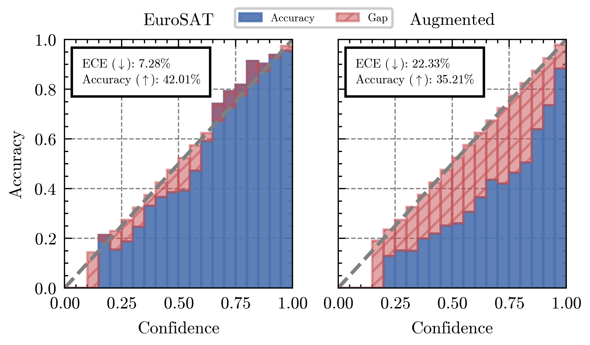
Figure 4: Reliability diagrams of CLIP-ViT-B-16 for EuroSat and its augmented version, generated following Sec.3.1.

Nevertheless, we highlight an additional caveat about satellite imagery which is particularly detrimental for Zero, and relates to the base model error over augmentations. Recall that, in Zero, the usage of $\overline{p}$ is backed by theoretical motivations and the manual adaptation of the temperature is supported by two concurrent observations: augmentations-induced overconfidence and a comparable error rate between source and augmented images. Simply put, the latter condition is not verified for satellite imagery. To show this phenomenon, we follow the experimental setup of Sec.3.1 and examine the reliability diagrams of EuroSAT[10] and of its augmented counterpart in Figure 4. As per Section 3.1, we display the ECE and the Top1-Accuracy on each version of the dataset. From this perspective, one can note that the base model error largely increases, in this domain, when augmented views are present. The accuracy on source images is $42.01\%$, dropping to $35.21\%$ simply due to augmentations.

Both observations, combined, suggest that crafting augmentations for satellite imagery requires an ad-hoc treatment, which makes it a controversial benchmark for TTA.

Appendix F Additional Implementation Details

Table 6: Standard deviations of Zero for Fine-grained classification. Each cell refers to Tab. 2.

Method	FLWR	DTD	PETS	CARS	UCF	CAL	FOOD	SUN	AIR
CLIP-ViT-B-16
Zero	$\pm$0.29	$\pm$0.26	$\pm$0.18	$\pm$0.28	$\pm$0.17	$\pm$0.12	$\pm$0.08	$\pm$0.11	$\pm$0.26
Zero+Ensemble	$\pm$0.06	$\pm$0.21	$\pm$0.06	$\pm$0.24	$\pm$0.20	$\pm$0.15	$\pm$0.11	$\pm$0.06	$\pm$0.11
MaPLe
Zero	$\pm$0.78	$\pm$0.97	$\pm$0.22	$\pm$0.38	$\pm$0.10	$\pm$0.29	$\pm$0.09	$\pm$0.62	$\pm$0.11
CLIP-ViT-B-16 + CLIP-ViT-L-14
Zero	$\pm$0.09	$\pm$0.16	$\pm$0.13	$\pm$0.12	$\pm$0.05	$\pm$0.08	$\pm$0.05	$\pm$0.05	$\pm$0.24

Standard deviations. To complement the results on Fine-grained classification, we report the standard deviation of Zero computed over 3 runs with different seeds in Table 6. These are not reported together with the average top1-accuracy in Tab. 2 to avoid an excessively dense table. On average, standard deviations are very small, suggesting that regardless of the inherent randomness of data augmentations, Zero is relatively stable. Note that standard deviations in Group 2 (i.e., with MaPLe) are slightly greater than those in the other groups. This fact does not stem from Zero’s or MaPLe’s greater instability, but from an experimental detail which we report here for completeness: while only one set of weights is officially released for each CLIP version [27], Khattak et al. [14] released 3 sets of pretrained weights for MaPLe, varying on the seed. To avoid picking one, we associated a set of weights to each of our runs, hence results from slightly different initializations are computed to match the experimental setup of Samadh et al. [32] (PromptAlign).

Reproducibility of TTA methods. For section 4, we reproduced all methods using the source code provided by the authors with the hardware at our disposal. This was done to ensure that hardware differences did not interfere with a correct evaluation. We found that all TTA strategies are highly reproducible, with negligible differences (i.e., $\Delta<0.1$) which we omitted by reporting the numbers from the official papers. In case of larger differences, we reported reproduced results.

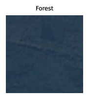
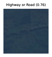
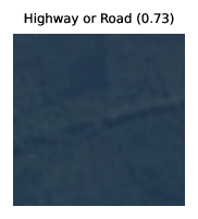
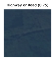
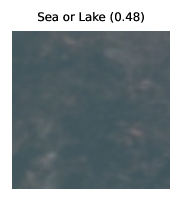
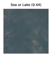
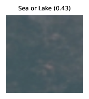
(a) Source Image	(b) Most confident	(c) 2nd most conf.	(d) 3rd most conf.

Figure 5: Examples of satellite imagery taken from EuroSAT[10], along with augmentations leading to high confident predictions. Column (a) reports source images with their label. Columns (b-d) report views sorted by entropy (lowest to highest), paired with the prediction and the confidence of CLIP-ViT-B-16 [30].

References

- Bossard et al. [2014] Lukas Bossard, Matthieu Guillaumin, and Luc Van Gool. Food-101–mining discriminative components with random forests. In European Conference on Computer Vision (ECCV), 2014.
- Cimpoi et al. [2014] Mircea Cimpoi, Subhransu Maji, Iasonas Kokkinos, Sammy Mohamed, and Andrea Vedaldi. Describing textures in the wild. In IEEE/CVF Conference on Computer Vision and Pattern Recognition (CVPR), 2014.
- Deng et al. [2009] Jia Deng, Wei Dong, Richard Socher, Li-Jia Li, Kai Li, and Li Fei-Fei. Imagenet: A large-scale hierarchical image database. In IEEE/CVF Conference on Computer Vision and Pattern Recognition (CVPR), 2009.
- Dosovitskiy et al. [2020] Alexey Dosovitskiy, Lucas Beyer, Alexander Kolesnikov, Dirk Weissenborn, Xiaohua Zhai, Thomas Unterthiner, Mostafa Dehghani, Matthias Minderer, Georg Heigold, Sylvain Gelly, et al. An image is worth 16x16 words: Transformers for image recognition at scale. In International Conference on Learning Representations (ICLR), 2020.
- Fei-Fei et al. [2004] Li Fei-Fei, Rob Fergus, and Pietro Perona. Learning generative visual models from few training examples: An incremental bayesian approach tested on 101 object categories. In IEEE/CVF Conference on Computer Vision and Pattern Recognition Workshops (CVPR-W). IEEE, 2004.
- Gandelsman et al. [2022] Yossi Gandelsman, Yu Sun, Xinlei Chen, and Alexei Efros. Test-time training with masked autoencoders. Advances in Neural Information Processing Systems (NeurIPS), 2022.
- Guo et al. [2017] Chuan Guo, Geoff Pleiss, Yu Sun, and Kilian Q Weinberger. On calibration of modern neural networks. In International Conference on Machine Learning (ICML), 2017.
- Hardt and Sun [2024] Moritz Hardt and Yu Sun. Test-time training on nearest neighbors for large language models. In International Conference on Learning Representations (ICLR), 2024.
- He et al. [2016] Kaiming He, Xiangyu Zhang, Shaoqing Ren, and Jian Sun. Deep residual learning for image recognition. In IEEE/CVF Conference on Computer Vision and Pattern Recognition (CVPR), 2016.
- Helber et al. [2019] Patrick Helber, Benjamin Bischke, Andreas Dengel, and Damian Borth. Eurosat: A novel dataset and deep learning benchmark for land use and land cover classification. IEEE Journal of Selected Topics in Applied Earth Observations and Remote Sensing, 12(7), 2019.
- Hendrycks et al. [2021a] Dan Hendrycks, Steven Basart, Norman Mu, Saurav Kadavath, Frank Wang, Evan Dorundo, Rahul Desai, Tyler Zhu, Samyak Parajuli, Mike Guo, et al. The many faces of robustness: A critical analysis of out-of-distribution generalization. In IEEE/CVF International Conference on Computer Vision (ICCV), 2021a.
- Hendrycks et al. [2021b] Dan Hendrycks, Kevin Zhao, Steven Basart, Jacob Steinhardt, and Dawn Song. Natural adversarial examples. In IEEE/CVF Conference on Computer Vision and Pattern Recognition (CVPR), 2021b.
- Jia et al. [2021] Chao Jia, Yinfei Yang, Ye Xia, Yi-Ting Chen, Zarana Parekh, Hieu Pham, Quoc Le, Yun-Hsuan Sung, Zhen Li, and Tom Duerig. Scaling up visual and vision-language representation learning with noisy text supervision. In International Conference on Machine Learning (ICML), 2021.
- Khattak et al. [2023] Muhammad Uzair Khattak, Hanoona Rasheed, Muhammad Maaz, Salman Khan, and Fahad Shahbaz Khan. Maple: Multi-modal prompt learning. In IEEE/CVF Conference on Computer Vision and Pattern Recognition (CVPR), 2023.
- Kimura [2021] Masanari Kimura. Understanding test-time augmentation. In International Conference on Neural Information Processing (ICONIP). Springer, 2021.
- Krause et al. [2013] Jonathan Krause, Michael Stark, Jia Deng, and Li Fei-Fei. 3d object representations for fine-grained categorization. In IEEE/CVF International Conference on Computer Vision Workshops (ICCV-W), 2013.
- Kuncheva [2014] Ludmila I Kuncheva. Combining pattern classifiers: methods and algorithms. 2014.
- Lee et al. [2024] Jonghyun Lee, Dahuin Jung, Saehyung Lee, Junsung Park, Juhyeon Shin, Uiwon Hwang, and Sungroh Yoon. Entropy is not enough for test-time adaptation: From the perspective of disentangled factors. In International Conference on Learning Representations (ICLR), 2024.
- Li and Liang [2021] Xiang Lisa Li and Percy Liang. Prefix-tuning: Optimizing continuous prompts for generation. In Proceedings of the 59th Annual Meeting of the Association for Computational Linguistics and the 11th International Joint Conference on Natural Language Processing (Volume 1: Long Papers), 2021.
- Liu et al. [2024] Zichen Liu, Hongbo Sun, Yuxin Peng, and Jiahuan Zhou. Dart: Dual-modal adaptive online prompting and knowledge retention for test-time adaptation. In AAAI Conference on Artificial Intelligence (AAAI), 2024.
- Ma et al. [2024] Xiaosong Ma, Jie Zhang, Song Guo, and Wenchao Xu. Swapprompt: Test-time prompt adaptation for vision-language models. Advances in Neural Information Processing Systems (NeurIPS), 2024.
- Maji et al. [2013] Subhransu Maji, Esa Rahtu, Juho Kannala, Matthew Blaschko, and Andrea Vedaldi. Fine-grained visual classification of aircraft. arXiv preprint arXiv:1306.5151, 2013.
- Mayilvahanan et al. [2023] Prasanna Mayilvahanan, Thaddäus Wiedemer, Evgenia Rusak, Matthias Bethge, and Wieland Brendel. Does clip’s generalization performance mainly stem from high train-test similarity? In International Conference on Learning Representations (ICLR), 2023.
- Nilsback and Zisserman [2008] Maria-Elena Nilsback and Andrew Zisserman. Automated flower classification over a large number of classes. In Indian conference on computer vision, graphics & image processing. IEEE, 2008.
- Niu et al. [2022] Shuaicheng Niu, Jiaxiang Wu, Yifan Zhang, Yaofo Chen, Shijian Zheng, Peilin Zhao, and Mingkui Tan. Efficient test-time model adaptation without forgetting. In International Conference on Machine Learning (ICML), 2022.
- Niu et al. [2023] Shuaicheng Niu, Jiaxiang Wu, Yifan Zhang, Zhiquan Wen, Yaofo Chen, Peilin Zhao, and Mingkui Tan. Towards stable test-time adaptation in dynamic wild world. In International Conference on Learning Representations (ICLR), 2023.
- [27] OpenAI. Clip. URL https://github.com/openai/CLIP.
- Parkhi et al. [2012] Omkar M Parkhi, Andrea Vedaldi, Andrew Zisserman, and CV Jawahar. Cats and dogs. In IEEE/CVF Conference on Computer Vision and Pattern Recognition (CVPR), 2012.
- Paszke et al. [2019] Adam Paszke, Sam Gross, Francisco Massa, Adam Lerer, James Bradbury, Gregory Chanan, Trevor Killeen, Zeming Lin, Natalia Gimelshein, Luca Antiga, et al. Pytorch: An imperative style, high-performance deep learning library. Advances in Neural Information Processing Systems (NeurIPS), 32, 2019.
- Radford et al. [2021] Alec Radford, Jong Wook Kim, Chris Hallacy, Aditya Ramesh, Gabriel Goh, Sandhini Agarwal, Girish Sastry, Amanda Askell, Pamela Mishkin, Jack Clark, et al. Learning transferable visual models from natural language supervision. In International Conference on Machine Learning (ICML), 2021.
- Recht et al. [2019] Benjamin Recht, Rebecca Roelofs, Ludwig Schmidt, and Vaishaal Shankar. Do imagenet classifiers generalize to imagenet? In International Conference on Machine Learning (ICML), 2019.
- Samadh et al. [2023] Jameel Hassan Abdul Samadh, Hanan Gani, Noor Hazim Hussein, Muhammad Uzair Khattak, Muzammal Naseer, Fahad Khan, and Salman Khan. Align your prompts: Test-time prompting with distribution alignment for zero-shot generalization. In Advances in Neural Information Processing Systems (NeurIPS), 2023.
- Schuhmann et al. [2022] Christoph Schuhmann, Romain Beaumont, Richard Vencu, Cade Gordon, Ross Wightman, Mehdi Cherti, Theo Coombes, Aarush Katta, Clayton Mullis, Mitchell Wortsman, et al. Laion-5b: An open large-scale dataset for training next generation image-text models. Advances in Neural Information Processing Systems (NeurIPS), 2022.
- Shanmugam et al. [2021] Divya Shanmugam, Davis Blalock, Guha Balakrishnan, and John Guttag. Better aggregation in test-time augmentation. In IEEE/CVF International Conference on Computer Vision (ICCV), 2021.
- Shapley and Grofman [1984] Lloyd Shapley and Bernard Grofman. Optimizing group judgmental accuracy in the presence of interdependencies. Public Choice, 1984.
- Sharma et al. [2018] Piyush Sharma, Nan Ding, Sebastian Goodman, and Radu Soricut. Conceptual captions: A cleaned, hypernymed, image alt-text dataset for automatic image captioning. In Proceedings of the 56th Annual Meeting of the Association for Computational Linguistics (Volume 1: Long Papers), 2018.
- Shu et al. [2022] Manli Shu, Weili Nie, De-An Huang, Zhiding Yu, Tom Goldstein, Anima Anandkumar, and Chaowei Xiao. Test-time prompt tuning for zero-shot generalization in vision-language models. Advances in Neural Information Processing Systems (NeurIPS), 2022.
- Singh et al. [2022] Amanpreet Singh, Ronghang Hu, Vedanuj Goswami, Guillaume Couairon, Wojciech Galuba, Marcus Rohrbach, and Douwe Kiela. Flava: A foundational language and vision alignment model. In IEEE/CVF Conference on Computer Vision and Pattern Recognition (CVPR), 2022.
- Son and Kang [2023] Jongwook Son and Seokho Kang. Efficient improvement of classification accuracy via selective test-time augmentation. Information Sciences, 2023.
- Soomro et al. [2012] Khurram Soomro, Amir Roshan Zamir, and Mubarak Shah. Ucf101: A dataset of 101 human actions classes from videos in the wild. arXiv preprint arXiv:1212.0402, 2012.
- Sui et al. [2024] Elaine Sui, Xiaohan Wang, and Serena Yeung-Levy. Just shift it: Test-time prototype shifting for zero-shot generalization with vision-language models. arXiv preprint arXiv:2403.12952, 2024.
- Sun et al. [2020] Yu Sun, Xiaolong Wang, Zhuang Liu, John Miller, Alexei Efros, and Moritz Hardt. Test-time training with self-supervision for generalization under distribution shifts. In International Conference on Machine Learning (ICML), 2020.
- Tomar et al. [2023] Devavrat Tomar, Guillaume Vray, Behzad Bozorgtabar, and Jean-Philippe Thiran. Tesla: Test-time self-learning with automatic adversarial augmentation. In IEEE/CVF Conference on Computer Vision and Pattern Recognition (CVPR), 2023.
- Wang et al. [2021] Dequan Wang, Evan Shelhamer, Shaoteng Liu, Bruno Olshausen, and Trevor Darrell. Tent: Fully test-time adaptation by entropy minimization. In International Conference on Learning Representations (ICLR), 2021.
- Wang et al. [2019] Haohan Wang, Songwei Ge, Zachary Lipton, and Eric P Xing. Learning robust global representations by penalizing local predictive power. Advances in Neural Information Processing Systems (NeurIPS), 2019.
- Wang et al. [2022] Qin Wang, Olga Fink, Luc Van Gool, and Dengxin Dai. Continual test-time domain adaptation. In IEEE/CVF Conference on Computer Vision and Pattern Recognition (CVPR), 2022.
- Xiao et al. [2010] Jianxiong Xiao, James Hays, Krista A Ehinger, Aude Oliva, and Antonio Torralba. Sun database: Large-scale scene recognition from abbey to zoo. In IEEE/CVF Conference on Computer Vision and Pattern Recognition (CVPR), 2010.
- Yuan et al. [2023] Longhui Yuan, Binhui Xie, and Shuang Li. Robust test-time adaptation in dynamic scenarios. In IEEE/CVF Conference on Computer Vision and Pattern Recognition (CVPR), 2023.
- Zancato et al. [2023] Luca Zancato, Alessandro Achille, Tian Yu Liu, Matthew Trager, Pramuditha Perera, and Stefano Soatto. Train/test-time adaptation with retrieval. In IEEE/CVF Conference on Computer Vision and Pattern Recognition (CVPR), 2023.
- Zanella and Ayed [2024] Maxime Zanella and Ismail Ben Ayed. On the test-time zero-shot generalization of vision-language models: Do we really need prompt learning? arXiv preprint arXiv:2405.02266, 2024.
- Zhai et al. [2023] Xiaohua Zhai, Basil Mustafa, Alexander Kolesnikov, and Lucas Beyer. Sigmoid loss for language image pre-training. In IEEE/CVF International Conference on Computer Vision (ICCV), 2023.
- Zhang et al. [2022] Marvin Zhang, Sergey Levine, and Chelsea Finn. Memo: Test time robustness via adaptation and augmentation. Advances in Neural Information Processing Systems (NeurIPS), 2022.
- Zhao et al. [2024] Shuai Zhao, Xiaohan Wang, Linchao Zhu, and Yi Yang. Test-time adaptation with CLIP reward for zero-shot generalization in vision-language models. In International Conference on Learning Representations (ICLR), 2024.
- Zhou et al. [2022a] Kaiyang Zhou, Jingkang Yang, Chen Change Loy, and Ziwei Liu. Conditional prompt learning for vision-language models. In IEEE/CVF Conference on Computer Vision and Pattern Recognition (CVPR), 2022a.
- Zhou et al. [2022b] Kaiyang Zhou, Jingkang Yang, Chen Change Loy, and Ziwei Liu. Learning to prompt for vision-language models. International Journal of Computer Vision (IJCV), 2022b.