New horizon symmetries, hydrodynamics, and quantum chaos
Abstract
We generalize the formulation of horizon symmetries presented in previous literature to include diffeomorphisms that can shift the location of the horizon. In the context of the AdS/CFT duality, we show that horizon symmetries can be interpreted on the boundary as emergent low-energy gauge symmetries. In particular, we identify a new class of horizon symmetries that extend the so-called shift symmetry, which was previously postulated for effective field theories of maximally chaotic systems. Additionally, we comment on the connections of horizon symmetries with bulk calculations of out-of-time-ordered correlation functions and the phenomenon of pole-skipping.
Keywords: Asymptotic symmetries, horizon symmetries, black holes, hydrodynamics, chaos
I Introduction
Asymptotic symmetries are local symmetries that do not vanish at infinity and preserve the boundary conditions. They are believed to represent physical symmetries of the system. For instance, in the context of the AdS/CFT duality, asymptotic symmetries in an asymptotic AdS spacetime correspond to global symmetries of the boundary system.
For a black hole geometry, the focus is often on the physics outside the horizon. In this case, it is convenient to treat the event horizon as a “boundary” in an effective sense as it has been done, for example, in the so-called membrane paradigm [1]. It is natural to extend the discussion of asymptotic symmetries to an event horizon and consider diffeomorphisms that preserve the horizon of a black hole geometry [2, 3, 4, 5, 6], as well as their physical implications. See e.g., [7, 8, 9, 10, 11, 12, 13, 14] for further discussions on this topic and [15, 16, 17, 18, 19, 20, 21] for applications to the black hole microstate counting. Since a horizon is not a genuine physical boundary, such horizon-preserving diffeomorphisms are not true asymptotic symmetries, and their precise physical interpretations remain unclear. Below we will follow the standard terminology and refer to them as “horizon symmetries”.
To probe physical interpretations and implications of horizon symmetries, it is helpful to consider them in a familiar context. In this paper, we consider horizon symmetries in an eternal black hole in AdS and seek a precise physical interpretation in terms of the boundary CFT. We will first generalize the formulation of horizon symmetries given in [5, 6, 12], then show that they can be interpreted in the boundary theory as emergent low-energy gauge symmetries, and finally discuss their connections with hydrodynamics and maximal chaos.
The main results of this paper can be summarized as follows:
-
1.
We define horizon symmetries as bulk diffeomorphisms that preserve both the null vector field and its non-affine parameter on the horizon. These include those that can move the location of the horizon, i.e. without restricting to diffeomorphisms that lie along the horizon as in [22].
For a stationary black hole in a suitable coordinate system, the horizon symmetries are
(1) (2) where are horizon coordinates, , , , and are generic functions of the spatial coordinates , is a constant that depends on the specific black hole metric, and is the non-affinity parameter. The novel symmetry is parameterized by and is proportional to an exponentially growing term .
-
2.
We show that the horizon symmetries (1) and (2) in fact correspond to gauge symmetries of the dual boundary hydrodynamic and maximally chaotic effective field theory. In particular, the symmetries parametrized by and correspond to certain gauge symmetries of any hydrodynamic effective field theory defined in [23, 24, 25, 26, 27]. The symmetries parameterized by and in (1), dubbed as shift symmetries, correspond to symmetries of maximally chaotic systems as proposed by [28, 29].
This claim relies on the fact that both the hydrodynamic [23, 24, 25, 26, 27] and maximally chaotic effective field theories [28, 29] are based on the definition of appropriate hydrodynamical variables. Their gravitational counterpart has been discussed in [30, 31, 32] which identify the dual field theory fluid variables with the relative embedding between the boundary and the horizon. Horizon symmetry transformations, like (1) and (2), then lead directly to symmetry transformations of the hydrodynamical variables. Given that horizon symmetries are bulk diffeomorphisms, the corresponding symmetry transformations of the hydrodynamical variables are then identified as gauge symmetries of the dual boundary hydrodynamic and chaotic effective field theory.
-
3.
Two special features of maximally chaotic systems as the ones arising in the context of holography [33, 34, 35] and SYK models [36, 37, 38, 39] are the exponential growth of Out-of-Time Ordered Correlators (OTOCs) and the pole-skipping phenomenon [40, 28, 41]. We show that the horizon symmetries parameterized by can be used to create shock wave geometries, analogous to the ones analyzed in [33, 34, 35] that lead to the exponential growth of OTOCs in holographic systems. Moreover, we will comment on the connection between horizon symmetries and the pole-skipping phenomenon in the energy density retarded two-point function.
This paper is organized as follows. In Section II we start by illustrating our setup and defining the generators that preserve the horizon structure. In particular, we will show how symmetries like (1) and (2) arise as symmetries of black hole horizons. Then, we construct the holographic dual degrees of freedom for boundary hydrodynamics in Section III. We show that these objects inherit the horizon symmetries (1) and (2), establishing the correspondence and the interpretation of the horizon symmetries as symmetries of the dual fluid dynamical variables. In Section IV we use the horizon symmetries to generate shock wave geometries and elaborate on their connection to the chaotic features of OTOCs as well as the pole-skipping phenomenon. We conclude with a summary and discussion in Section V. Details of some of the derivations are deferred to Appendices A-C.
II Formulation of horizon symmetries
II.1 Setup
Consider a -dimensional black hole spacetime with a horizon111We focus on black hole horizons despite much of this discussion can be applied to any null surface. denoted as . The spacetime is described by a metric with coordinates . can be specified by a set of embedding functions in , where denote intrinsic coordinates on . We will denote bulk quantities with capital latin indices and horizon quantities with .
The intrinsic metric on can be written as
| (3) |
where is an equality evaluated at the horizon. By definition, is degenerate, and has a single eigenvector with zero eigenvalue,
| (4) |
Through , we can push forward to a spacetime vector field ,
| (5) |
The vector will be assumed to have a smooth extension away from , and our discussion below will not depend on its extension. By definition is null on , that is
| (6) |
and it is normal to as (4) implies that
| (7) |
Moreover, can be shown to satisfy the geodesics equation
| (8) |
with some scalar (non-affine parameter).
There is no intrinsic way to normalize , and under a rescaling,
| (9) |
where is an arbitrary scalar on the horizon, and and denote the Lie derivative along and respectively. Equations (9) define an equivalence relation: the pairs related by such rescalings should be viewed as being equivalent. The equivalence class of the pair under (9) is referred to as the horizon structure, see, e.g., [22]. Later, we will often use the freedom (9) to fix
| (10) |
It is convenient to introduce another spacetime 1-form that is null on , satisfying
| (11) |
We can pull back to to define a 1-form ,
| (12) |
Using (11), we can also define a projector
| (13) |
The quantity is asymmetric; acting with it on a vector from the left projects to the space orthogonal to , while acting from the right projects to the space orthogonal to . We can also define a symmetric, codimension-two, transverse projector
| (14) |
which acts as a projector onto the base space of the horizon . That is, if we assume the horizon to have a topology , where is the null direction, projects onto the space .
Notice that the choice of is not unique. It is always possible to shift its value as long as (11) is satisfied as we discuss in detail in Appendix A. Our discussion will not depend on a specific choice of .
The most general horizon metric can be written in the form
| (15) |
where is a non-degenerate spatial metric. We then have
| (16) | |||
| (17) |
where is an arbitrary normalization. Suppose we choose the horizon coordinates such that
| (18) |
then , and
| (19) |
II.2 Review
In this subsection we review the formulation of horizon symmetries given in [22]. Consider an infinitesimal diffeomorphism on generated by a vector field under which
| (20) |
A general does not preserve the horizon structure specified by the equivalence class of the pair . The horizon symmetries of [22] are defined by those that preserve the horizon structure. That is, the corresponding lies in the equivalence class of . This leads to the requirements
| (21) | |||
| (22) |
for some infinitesimal scalar function on .
To see the implications of the conditions (21) and (22), it is convenient to decompose into a part that is along the null direction and a part that is orthogonal to it,
| (23) |
where and are functions of the horizon coordinates. These functions have been referred to as supertranslations and superrotations respectively, in analogy with the asymptotic symmetry structure and terminology of flat spacetime. It can be shown that, with the decomposition (23), equations (21) and (22) become the following conditions on and ,
| (24) | |||
| (25) |
see, e.g., [22, 14]. With (24) written as
| (26) |
equation (25) can be written alternatively as
| (27) |
While in (25) there is an apparent dependence on (and thus the choice of ), it can be explicitly verified that there is, in fact, none. See Appendix A for details.
To explicitly see the form of the horizon symmetry implied by (26) and (27), we can choose the normalization of and the intrinsic coordinates such that (10) and (18) hold. Then, with the simple choice of , equation (23) has the form
| (28) |
In this case, (26) becomes
| (29) |
and equation (27) reduces to
| (30) |
Equations (29)–(30) are solved by
| (31) | |||
| (32) |
where , and are arbitrary functions of the spatial horizon coordinates .
The explicit form of the horizon symmetries (31) and (32) has also been derived before in [5, 6], where the authors considered black hole horizons expressed in Gaussian null coordinates and defined the horizon symmetries to be those bulk diffeomorphisms that preserve these coordinates. Other proposals for horizon symmetries include [42, 19, 12].
II.3 New horizon symmetries
In this subsection, we present our formulation of horizon symmetries that leads to additional symmetries beyond those given in (31) and (32). Consider an infinitesimal variation of the metric , which induces a variation of the metric on the horizon hypersurface ,
| (33) |
We say that the variation preserves the horizon structure if the following two conditions are satisfied:
-
1.
The vector on has still zero eigenvalue under the new horizon metric, i.e.,
(34) which is equivalent to
(35) for some infinitesimal function defined on .
-
2.
We require to be unchanged under the new metric, i.e., with denoting the covariant derivative associated with ,
(36) which can also be written as
(37)
Now suppose the metric variation is generated by a diffeomorphism, i.e.,
| (38) |
for some infinitesimal vector field . We say that generates a horizon symmetry if (38) preserves the horizon structure as defined above. This requirement translates into the following two conditions
| (39) | |||
| (40) |
To derive equation (39), we use that
| (41) |
Combined with (35), this expression leads to
| (42) |
which readily gives (39) with given by
| (43) |
II.4 along the horizon
To see the implications of (39) and (40), we consider first along the horizon, i.e.,
| (45) |
In this case, the diffeomorphisms at the horizon can be thought of as being intrinsic to the hypersurface and, as we will show below, our formulation of the horizon symmetries is equivalent to that of Sec. II.2. In the next subsection, we will consider the general case with , allowing us to derive new horizon symmetries.
For satisfying (45), we can “pull it back” to as follows
| (46) |
where is the inverse of in the subspace orthogonal to (recall that )222We may say that the subspace spanned by does not contain while that spanned by does not contain ., i.e., it is the matrix satisfying
| (47) |
With (45), (34) can be written as
| (48) | |||
| (49) |
where we have used that for any vector of the form ,
| (50) | |||
| (51) |
From (49) we conclude that (34) (and therefore (39)) is equivalent to
| (52) |
for some infinitesimal function , which recovers (21).
II.5 General case
We now consider a general vector field which we parameterize as follows
| (62) |
where , , and are functions of the horizon coordinates, , and lies along . The horizon symmetry conditions on are (39) and (40). It can be shown that (see Appendix B for detailed derivations) equation (39) reduces to
| (63) | |||
| (64) |
for some function which can be written as
| (65) |
while equation (40) reduces to
| (66) | |||
| (67) |
with
| (68) |
We can also rewrite (66) (by using (65) in (66)) as
| (69) | |||
| (70) |
Equations (63), (64), and (66) constitute a central result of our work. They are constraint equations that select a specific class of diffeomorphisms which we call horizon symmetries. They are parameterized by the supertranslations , the superrotations , and the radial displacement . The part dependent on leads to the new horizon symmetry and will play a central role in characterizing the chaotic regime of a black hole as we will see explicitly later on.
The authors of [22] always worked in a regime where which allowed them to derive the constraint equations (24) and (25) that lead to (31) and (32). Moreover, they always imposed by requiring . This latter condition is equivalent to a constraint on terms in away from the horizon, without affecting the form of and . The authors of [6], while allowing a general radial displacement and deriving similar intermediate equations to ours in Gaussian null coordinates, always effectively imposed by requiring independence of their horizon symmetries from the fields parameterizing the horizon metric (apart from ). After additionally requiring that , they derived equations (31) and (32). Their proposal of horizon symmetries also constrained some components of away from the horizon.
II.6 Simplifications of the horizon symmetry equations
We now further simplify (63)–(64) and (66) by choosing a convenient set of horizon coordinates. Recall that
| (71) |
Therefore, introducing
| (72) |
we have
| (73) |
We should view quantities all as functions defined on , i.e., they are functions of the horizon coordinates . The quantities introduced in (68) should be evaluated on the horizon and thus are also considered as functions of .
We will again choose the normalization of and the intrinsic coordinates such that (10) and (18) hold. We will choose such that , and thus where is a spatial vector on the horizon. Similarly, we have
| (74) |
where is also a spatial vector on the horizon such that .
Equation (63) then becomes,
| (75) |
where is a generic function of the spatial horizon coordinates . This exponentially growing solution is the new horizon symmetry, key to our later discussion in connection to many-body quantum chaos in Sec. IV.
Equation (64) can be written as
| (76) | |||
| (77) |
which implies that
| (78) |
Finally, equation (66) becomes
| (79) | |||
| (80) |
It is not possible to solve equations (78) and (79) in full generality as they still depend on the details of the horizon metric , on and . In the next subsection, we will choose a specific example that will allow us to obtain an explicit form of the horizon symmetries.
II.7 An explicit example
Consider the boosted black brane solution in AdSd+1. Its metric in Eddington-Finkelstein coordinates has the form
| (81) |
where is a constant vector satisfying , and the indices are raised by the Minkowski metric , and
| (82) | |||
| (83) |
Here, a constant is the radial location of the horizon, is the AdS scale, and is a projector in the directions that are orthogonal to , that is .
With the embedding function where the horizon coordinates are taken to be the same as the spacetime coordinates , the induced metric on the horizon is
| (84) |
which gives
| (85) |
with an arbitrary normalization factor . We can also readily calculate
| (86) |
where
| (87) |
is the non-affine parameter for the Killing vector , and is the (constant) inverse temperature of the black brane. For the condition (10) to hold, we choose a constant that satisfies
| (88) |
The horizon coordinates satisfying the conditions (18) are obtained from via the Lorentz boost that takes to ,
| (89) |
The inverse transformation is
| (90) |
which gives the embedding functions . In terms of , the horizon metric has the form
| (91) |
with . We also choose
| (92) |
which leads to the projector
| (93) |
The infinitesimal diffeomorphism vector can then be decomposed using (62) as
| (94) | |||
| (95) |
where we have introduced
| (96) | |||
| (97) |
Moreover, we have
| (98) | |||
| (99) |
which gives
| (100) | |||
| (101) |
Equation (75) can now be written as
| (102) |
where is given by (89). Equation (78) becomes
| (103) | |||
| (104) |
and equation (79) becomes
| (105) | |||
| (106) |
A special case is the black brane with , for which we have
| (107) | |||
| (108) | |||
| (109) |
II.8 Passive perspective
Before concluding this section, we comment on the passive perspective of the horizon symmetries. Instead of varying the metric with the embedding fixed as we have done in Section II.3 with , we can alternatively fix the metric and change the embedding of the horizon. In the new coordinates, the embedding functions become
| (110) |
where is the vector parameterizing linearized diffeomorphisms and should be evaluated at the horizon.
III Hydrodynamical interpretation
We now consider a gravity system in asymptotically AdSd+1 spacetime with a strongly coupled conformal field theory (CFT) dual. In particular, we will consider a black hole in AdSd+1, dual to a boundary system at a finite temperature. For definiteness we take the boundary to be with Minkowski metric .333The discussion can be generalized straightforwardly to a curved boundary metric. In what follows, we will argue that the horizon symmetries can be interpreted as emergent gauge symmetries of an effective field theory (quantum hydrodynamics) of the boundary system.
III.1 Review
We start by reviewing some necessary ingredients for a theory of (quantum) hydrodynamics. In the effective field theory approach to hydrodynamics based on an action principle developed in [24, 27, 44] (see also [23, 25, 26]), the dynamical variables are maps between the fluid spacetime labeled by the coordinates and the physical spacetime with coordinates . The spatial coordinates in the fluid spacetime label fluid elements while can be considered as their “internal time”. For a fixed , gives the spacetime trajectory of a fluid element with label , parameterized by . We denote the inverse map of as , which describes the fluid elements passing through the point at time . The dynamical variables such as the velocity field and temperature of the more conventional approach can be expressed in terms of as
| (115) |
See, e.g., [44] for more details and references.
An important element in the formulation of the effective action of hydrodynamics is that the action should be invariant under the “gauge symmetries”
| (116) |
where and are arbitrary functions of the spatial variables . The symmetries (116) can be interpreted as a reparameterization freedom of the fluid variables and of their internal time. They played a crucial role in constraining the form of the hydrodynamic effective action and the resulting correlation functions.
For a strongly coupled CFT at finite temperature , physics at distances and time scales much greater than is described by hydrodynamics, usually formulated in a derivative expansion with an effective expansion parameter . Nevertheless, the recent reformulation of hydrodynamics indicates that the theory can in fact be extended to scales , well beyond the usual regime of validity of hydrodynamics. Such a theory, called quantum hydrodynamics, is nonlocal and yet may have predictive power.
In fact, in [28, 29], quantum hydrodynamics was used to postulate an effective field theory for maximally chaotic systems.444The effective field theory of [28, 29] was constructed for systems with only energy conservation (no momentum conservation). A full effective field theory for translationally invariant maximally chaotic systems has not yet been constructed. In addition to (116), it was assumed that such a theory also possesses a shift symmetry of the form
| (117) |
that leads to a transformation of the velocity field as follows
| (118) | |||
| (119) |
where and are generic functions of the boundary spatial coordinates .555In writing this equation, we imposed of [28] to be to match our notation. The difference is in the choice of the equilibrium configuration. As we will see shortly, we impose while [28] have .
III.2 Horizon symmetries as gauge symmetries of quantum hydrodynamics
Here we show that the symmetries used to formulate hydrodynamics (116), as well as the shift symmetry (117) postulated for maximally chaotic systems, can be understood on the gravity side as horizon symmetries in the context of the AdS/CFT correspondence.
For a holographic system in a local equilibrium state, hydrodynamical variables (or equivalently the inverse maps ) can be obtained from the relative embedding between the boundary (with coordinates ) and the horizon (with coordinates ) as developed in [30, 31, 32]. More explicitly, given a bulk metric , consider shooting a null geodesic with tangent vector from the boundary to the horizon. The geodesic leaves the boundary at , and reaches the horizon at point , establishing the map and its inverse .
The velocity field and temperature can then be obtained from the definition (115) in the effective field theory approach. Using the map , we can push forward the null vector defined on the horizon to a vector on the boundary,
| (120) |
where we have used our choice of the horizon coordinates (18). Below, we will see explicitly that by choosing in (10) to be
| (121) |
for an equilibrium configuration, obtained from (120) coincides with the boundary inverse temperature. Thus, we can interpret and defined by (120)–(121) respectively as the local fluid inverse temperature and velocity for a general non-equilibrium case.
Notice that the given definition of the map in gravity is not unique. Using the Fefferman-Graham coordinates near the boundary, we can parameterize in terms of a time-like vector as follows
| (122) |
The choice of corresponds to a choice of the local Lorentz frame characterizing the boundary fluid.
We now consider more explicitly how horizon symmetries act on the hydrodynamical variables or . For this purpose, it is convenient to write the bulk metric in terms of the Eddington-Finkelstein coordinates as follows
| (123) |
in which null geodesics represented by lines of are precisely those with the tangent vector at the boundary specified by (122), see [45]. We can also choose the radial coordinate so that lies at . The induced metric at the horizon can then be written as
| (124) |
With the horizon coordinates being specified by (10) and (18), the horizon embedding functions are given by and .
In (123), the radial geodesic starting from with tangent vector (122) is simply given by with a parameter along the geodesic. That is, starting from on the boundary, the horizon is reached at and the map is then given by
| (125) |
Thus the boundary local temperature and velocity field are given by
| (126) |
Notice that each gravity solution determines a solution of and , which can be defined without performing any derivative expansion. Thus the effective field theory of may be considered as “quantum hydrodynamics” which is valid for spacetime variations of order and goes beyond the usual effective theory arising in the context of the fluid/gravity correspondence.
Now consider making a horizon symmetry transformation generated by some infinitesimal vector field parameterized by (62). As discussed in Sec. II.8, we can equivalently describe the transformation in terms of a linearized shift in the embedding functions
| (127) |
with unchanged. More explicitly, we have
| (128) |
Since the metric does not change, the geodesic starting at now hits the horizon at where
| (129) |
and is the inverse of evaluated at . The new boundary to horizon map is given by
| (130) |
The new velocity field is then
| (131) |
Since horizon symmetry transformations are bulk diffeomorphisms, they take a gravity solution to another. Moreover, the two solutions should be physically equivalent. This implies that the corresponding transformations (130)–(131) should again be viewed as “gauge symmetries” of the dual effective field theory of quantum hydrodynamics. In particular, such transformations could in principle change the local boundary inverse temperature and velocity, and lead to nontrivial constraints on the hydrodynamic equations. Below we will look at an explicit example.
III.3 An explicit example
As an illustration of the above abstract discussion, we consider the boundary system on in a thermal equilibrium at inverse temperature , which is described in the bulk by the solution (81)–(83) with , i.e. with ,
| (132) | |||
| (133) |
The horizon is located at the constant value and the induced metric on is given by
| (134) |
The boundary inverse temperature is given by
| (135) |
Using the already derived relations (89), the horizon coordinates satisfying the conditions (10), (18) (88), and (121) are
| (136) |
Given the metric (132), we choose for the radial null geodesics defined in (122). In this way, a point on the boundary is simply mapped to . We then have
| (137) |
and thus the velocity field is given by
| (138) |
with the inverse temperature given by (135) as anticipated around (121).
The set of horizon symmetry transformations parameterized by the vector field was given in (94) and (107)–(109), which we copy here for convenience
| (139) | |||
| (140) | |||
| (141) | |||
| (142) |
From (131), we then find the transformation of the boundary inverse temperature and velocity field are given by
| (143) | |||
| (144) |
We note that and do not lead to any change in . They lead to a diffeomorphism on the horizon of the form
| (145) |
which matches the field theory symmetry of hydrodynamics (116). The velocity field transformation (143) matches the previous postulate (118) with our choice of given in (121) and . Equation (144) is instead a new prediction with respect to (119).
IV Implications for quantum chaos
In Section III, we discussed how horizon symmetries formulated in Section II lead to low-energy gauge symmetries in the effective field theory (quantum hydrodynamics) of the boundary theory in the context of the AdS/CFT correspondence. The symmetry transformations associated with the parameters and are related to symmetries of the dual hydrodynamic theory [27]. The symmetry transformations associated with parameters and are related to the shift symmetries (117) postulated in [28, 29] for maximally chaotic quantum many-body systems as we have seen explicitly towards the end of the previous section. We now comment in more detail on the implications of these symmetries on quantum chaos by considering two probes, the OTOCs and the phenomenon of pole-skipping.
In the effective field theory formulation of [28, 29], the shift symmetry associated with (i.e. the exponentially growing part) implies that the linearized hydrodynamic field , defined as , has an exponentially growing gauge symmetry transformation which in turn implies an exponentially growing propagator . This feature leads to the exponential growth of finite temperature OTOCs, , for two general scalar operators . Furthermore, invariance of the system under the shift symmetry associated with (i.e. the exponentially decreasing part) is crucial for the absence of the exponentially growing behavior in the time-ordered correlators (TOCs), . Given our identification of horizon symmetries with the symmetries of the dual quantum hydrodynamic theory, we thus see that the exponential growth of OTOCs (and the absence of the exponential growth of TOCs) for theories with a holographic dual has its gravitational origin in horizon symmetries.666Horizon symmetries in connection with quantum chaos have also been discussed in [43, 13].
In [28, 29], the stress-energy tensor is seen as a composite operator of the hydrodynamic fields. Therefore, the presence of the exponentially growing behavior in the two-point function of may cause concerns as it may lead to the exponential growth in correlation functions of the stress tensor too. This would imply instabilities that are generically not allowed. Nevertheless, in [28] it was further argued that the shift symmetries ensure that such an exponentially growing behavior does not appear in the correlation functions of the stress tensor through the phenomenon called pole-skipping [40, 28, 41]. We thus conclude that the pole-skipping phenomenon in holographic theories is also intimately related to horizon symmetries.777As we will elaborate more explicitly below, only pole-skipping in a particular channel of the stress tensor, the energy conservation channel, should be due to the horizon symmetries.
That the horizon plays a crucial role in both the exponential growth of OTOCs and the pole-skipping phenomenon has of course been well understood. In the original calculation of OTOCs from holography [33], the energy of small perturbations to a thermofield double state long in the past is exponentially blueshifted from the horizon, which leads to the exponential growth of the OTOCs. The pole-skipping phenomenon was discovered on the gravity side from an analysis of the Einstein equations near the horizon in [40] and elucidated in [41].
In this section, we elaborate a bit further on these gravity calculations from the perspective of horizon symmetries.
IV.1 Connection with the shock wave geometry
For a holographic system, an OTOC can be obtained from the dual bulk gravity system by calculating two-point functions of in a shock wave geometry generated by the operator inserted in the infinite past of a black hole geometry, see, e.g., [33, 46, 35]. We may view the shock wave as an effective description of multiple graviton exchanges between and , which can in turn be interpreted in the boundary system in terms of exchanges of the hydrodynamic modes corresponding to the stress tensor.
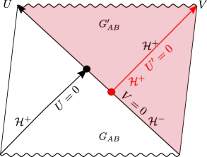
In this subsection, we show that the shock wave geometry of [47, 33, 46, 35] (see, e.g., Fig. 1) can be interpreted as being generated by a horizon symmetry transformation. More explicitly, we will show that near the horizon, the shock wave generated by inserting at early times may be viewed as patching together two spacetimes with metrics and along the trajectory of the quantum created by . Here is the black brane spacetime describing the equilibrium state, while is related to by a horizon symmetry transformation. In other words, we may say that an insertion generates a horizon symmetry transformation. We will now describe this connection in more detail using the example of (132).
For this purpose it is convenient to use the Kruzkal-Skezeres (KS) coordinates in terms of which the black brane metric (132) has the form
| (146) |
where the coordinates and are given as follows
| (147) |
and
| (148) |
In KS coordinates, the black hole’s future horizon is located at , while the past horizon is at .
The shock wave geometry generated by a high energy particle with trajectory similar to that used in [33, 46, 35, 47], is given by
| (149) |
where is the Heaviside stepfunction. It is described by an unperturbed black brane with a metric given in equation (146) for , while for the coordinates are shifted by where is given by
| (150) |
The function is determined by the Einstein’s equations
| (151) |
where is some constant, is the energy of the particle, and the exponential factor comes from a boost near the horizon.
Consider now the effect of the horizon symmetry transformation (140)-(142) parameterized by . Near the future horizon, this linearized888 Notice that we work at the linearized level in . With this approximation, one can probe boundary times for which the backreaction due to is substantial such that we can see the exponential growth similar to [33]. This aligns with expectations from [28, 29] for maximally chaotic quantum many-body systems. transformation can be expressed in terms of the KS coordinates as
| (152) | |||
| (153) | |||
| (154) |
Notice that at , the transformation in (152)-(154) reduce to that in (150) upon the identification near the future horizon.
One can use these transformations to construct a geometry with metric ,
| (155) |
described by the unperturbed black hole with metric (146) for , and by the metric (146) with the coordinate transformation in (152)-(154) for . Crucially, the geometry described by and the one described by are related by a coordinate transformation near the future horizon as follows
| (156) |
with
| (157) |
and upon linearization. In deriving (157) we have used the fact that the delta functions arising from derivatives on do not contribute as they are always multiplied by factors of near the future horizon.
Hence, near the future horizon, the two seemingly different shock wave metrics and are related by a diffeomorphism and are thus physically equivalent. Notice that to extend this argument beyond the near-horizon limit, one needs to know how the horizon symmetry transformation (140)-(142) acts away from the horizon. An interesting set of transformations are those for which . In this case, and are related by the coordinate transformation (157) even away from the future horizon. Consequently, gluing of to using the horizon symmetry serves as a solution-generating technique for the shock wave geometry created by a highly energetic particle released from the right boundary long in the past.
The procedure outlined above can also be used to construct the shock wave geometry created by a particle released from the left boundary that follows a null trajectory close to the future horizon located at . This geometry corresponds to gluing two halves of the unperturbed black hole along the slice with a shift in the direction . To generate this kind of geometry using horizon symmetries, it is necessary to consider the symmetries of the past horizon using outgoing EF coordinates and perform the gluing similar to the construction above.
Finally, we want to comment on the special case of . In this case, the coordinates and will not transform due to the vanishing of as can be seen from equation (106). Nevertheless, the coordinate will transform, and thus a shockwave geometry can be constructed. Therefore, we do expect that also for the OTOCs will grow exponentially due to the symmetry transformation related to .
IV.2 Connections with pole skipping
We now elaborate on the connection between the horizon symmetries and the phenomenon of pole skipping.
First, we review the argument of pole-skipping contained in [28]. There it was shown that the exponentially growing part of the symmetry in (117) parameterized by implies that the momentum space retarded two-point function of the linearized hydrodynamic mode has a pole in the upper half complex -plane at
| (158) |
which gives rise to the coordinate space behavior
| (159) |
where is the maximal Lyapunov exponent and is the butterfly velocity.
The stress tensor in the hydrodynamic effective field theory approach is expressed as a composite operator in terms of the hydrodynamic fields where . Therefore its correlation functions are determined by those of . However, the behavior (159), and thus the pole (158), cannot appear in the two-point functions of , and thus must be canceled through how depends on . Since is a physical observable, its dependence on must be invariant under the shift symmetries parameterized by and contained in (142), which are gauge symmetries. Working in the regime of no momentum conservation, it has been argued in [28] that the gauge invariance of in fact warrants that the pole (158) is always canceled in the retarded correlator of the energy density operator by the appearance of a zero at the same location. This is the phenomenon of pole-skipping.
Notice that while the pole in given in (158) is universal, the values of and the butterfly velocity depend on the specific theory and cannot be determined from symmetries. On the gravity side, their values depend on the specific background via the bulk equations of motion, see, e.g., [40, 41]. This can also be seen from the discussion on the shock wave geometries of the previous subsection. While the horizon symmetries allow any choice of , the explicit profile is determined through the shock wave equation (151) which in turn comes from the specific form of the Einstein equations. In fact, the solution to the shock wave equation determines the spatial dependence in (159), and thus the location of the skipped pole in (158). Indeed it was shown explicitly in [41] from an analysis of the Einstein equations near the horizon that precisely the shock wave equation (151) determines the location of in the pole-skipping phenomenon. Thus horizon symmetries lead to the phenomenon of pole-skipping and specify the frequency in (158), but more information is needed beyond horizon symmetries to determine and thus the full location of the pole.
We emphasize that in [28] the authors worked within the energy density conservation channel were the momentum dependence was explicitly turned off, that is . Thus, the Green’s function for was solely given in terms of its dependence on and there was no symmetry associated to coordinates in (117) and (119). Our prediction arising from horizon symmetries given in (144) could play a role in the construction of a complete effective field theory for maximally chaotic systems. In particular, including momentum dependence would lead to a contribution of the propagator even to and thus needs to be considered. The constraints on arising from (144) might be crucial to understand the pole-skipping phenomenon in a full effective field theory for maximally chaotic systems.
This expectation seems even more true in light of the pole-skipping phenomenon for holographic systems obtained directly from gravity calculations in [40, 41]. There, it was shown from a near horizon analysis of the Einstein’s equations of motion, that the pole-skipping phenomenon arises for every dimensionality of the bulk spacetime. Nevertheless, from our horizon symmetry analysis and from the arguments outlined in [28], it would seem that in dimensions there would be no pole-skipping phenomenon due to the absence of an exponentially growing symmetry transformation of as can be seen in (142) with given by (106). Thus, the prediction given in (144) could be pivotal in proving the pole-skipping phenomenon for holographic systems from an effective field theory approach. We reserve an explicit analysis of this point for future work.
Since the initial discussions of [40, 41] of the pole-skipping phenomenon in the sound channel (or energy diffusion channel in the absence of momentum conservation) associated to chaos, an infinite tower of pole-skipping points has been found in the lower half of the complex plane for all channels, and for many other types of fields, see, e.g., [48]. From the perspective of horizon symmetries considered in this paper, only the pole-skipping phenomenon associated with the energy density operator for (158) is implied by the horizon symmetries. The pole-skipping phenomenon in the other channels/fields, while clearly also having to do with the horizon dynamics, appears to be unrelated to the horizon symmetries identified in this work which should only affect hydrodynamic modes. Thus we would conclude the pole-skipping phenomenon in other fields and other gravitational channels likely arises from different physics.
V Conclusions and discussions
In this work, we generalized the discussion of [22, 5, 6] of horizon symmetries to a larger class and gave a boundary interpretation of the symmetries as the gauge symmetries of the dual quantum hydrodynamic theory in the context of the AdS/CFT correspondence. We worked out the symmetries in some simple examples and showed the existence of a new exponentially growing symmetry that has close connections with the behavior of OTOCs and the pole-skipping phenomenon.
In particular, we provided a new prediction for the gauge symmetries of any maximally chaotic effective field theory that has a gravitational dual. We showed that horizon symmetry transformations can be used as a solution generating technique to build up shock wave geometries as those arising in the holographic computations of OTOCs [33, 35]. Finally, we showed that the pole in in the pole-skipping phenomenon is universal and implied by the horizon symmetries, while the argument for the existence of a pole in is model-dependent and necessitates additional bulk information.
We now point out some interesting future directions. Among the most straightforward generalizations to consider are more general black holes, such as charged black holes and those corresponding to far-from-equilibrium states. It would also be useful to understand what happens to the horizon symmetries when including higher derivative or stringy corrections. The latter correspond to instances of non-maximal chaos which is subject of current ongoing research.
Another avenue is to consider spacetimes that are not asymptotically AdS since much of our discussion can be generalized to the case of other signs of the cosmological constant. In fact, the hydrodynamic degrees of freedom can also be defined as maps between the horizon and some timelike boundary that is embedded in the interior of the bulk spacetime, not necessarely at asymptotic infinity. In this way, it is possible to analyse the hydrodynamic and chaotic regime (quantum hydrodynamic) of a putative dual theory that lives on that timelike boundary without knowing the precise details of that theory and the bulk asymptotics. See, e.g., [49, 50, 51, 52, 53, 54] for the fluid/gravity correspondence of these so called Rindler fluids.
To have additional support to the findings of this work, it would be useful to extend the effective field theory for maximally chaotic systems formulated in [28, 29] to also include momentum conservation and derive the implications of the transformation of the spatial coordinates due to in (140) on the OTOCs and the phenomenon of pole-skipping. In particular, this could possibly help the issue arising in we highlighted at the end of Section IV.2. A more challenging task is to have an explicit derivation of the chaos effective action formulated in [28, 29] from holography using the methods developed in [31, 32], perhaps also generalizing the findings of [8].
In this paper, we have identified the gravitational dual to the gauge shift symmetries and the hydrodynamic symmetries. It would also be desirable to identify the gravitational dual and its relation to horizon symmetries of another symmetry appearing in the context of effective field theories of hydrodynamics: the one responsible for the entropy production [55]. See, e.g., [14, 56] for results in this direction. At the same time, one might wonder whether it is possible to identify gravitational and effective field theory symmetries related to the additional, infinite set of skipped poles found in [48] in various channels and for various fields.
It has been argued that horizon symmetries lead to local charges upon using the Wald-Zupas [57] or the Barnich and Brandt formalism [58] (see, e.g., [5, 6, 22]). It would be interesting to explore whether our horizon symmetries lead to local charges and what are their implications. In particular, local charges have to satisfy an integrability condition, that is they should be independent of the path taken in the so-called phase space, see, e.g., [59], for details. This problem has been circumvented in [18] by introducing edge modes: extra dynamical fields that ensure the resulting charges always respect the integrability condition. It would be interesting to explore possible relations between the gravitational edge modes of [18] and the fluid dynamic degrees of freedom described in these notes.
Acknowledgments
We would like to thank Ben Craps, Juan Hernandez, and Mikhail Khramtsov for useful discussions. NPF is supported by the European Commission through the Marie Sklodowska-Curie Action UniCHydro (grant agreement ID: 886540). NPF would also like to acknowledge support from the Center for Theoretical Physics and the Department of Physics at the Massachusetts Institute of Technology where most of the work was carried out. NPF was also supported in part by the National Science Foundation under the Grant No. PHY-1748958 to the Kavli Institute for Theoretical Physics (KITP) during the workshop refluids23 where part of the work was done. MK is supported by FWO-Vlaanderen project G012222N and by the VUB Research Council through the Strategic Research Program High-Energy Physics. HL is supported by the Office of High Energy Physics of U.S. Department of Energy under grant Contract Number DE-SC0012567 and DE-SC0020360 (MIT contract # 578218).
Appendix A Freedom in choosing
Having defined as the unique vector that satisfies on the horizon up to rescalings (9), there is yet a freedom in choosing the vector . This can be shown as follows. Consider a basis of tangent vectors to consisting of satisfying on
| (160) |
as well as the usual relations
| (161) |
We can always reparameterize and therefore on at will, so long as the above conditions are left invariant.
The most general transformation of this kind and can be parameterized as follows
| (162) |
then
| (163) | |||
| (164) |
We thus need to be an orthogonal matrix, which we can take to be the identity matrix. The other quantities are then set as
| (165) |
Thus, to summarize, we may always redefine on the horizon as follows
| (166) | |||
| (167) |
where is a generic vector while is its value evaluated at the horizon which can be decomposed into a part that is parallel to and a part that is orthogonal to it. The vector has to be taken as a function of the horizon coordinates. The redefinition (166) implies a redefinition of the projector too,
| (168) |
which will be useful later on.
The reparameterization freedom (166) and (168) is akin to the Carrollian boost transformation which arises in the context of ultra relativistic field theories. It has been shown that it also a symmetry of null surfaces when they are embedded in a Lorentzian spacetime of one dimension higher, see, e.g., [60].
A.1 Independence of
The arbitrariness in choosing seems to naively affect the horizon constraint equations derived in (24), (25) as well as in (63), (64), and (66). However, we will now show that this is not the case.
We start with the case where is tangent to the horizon, that is . In this case, and is decomposed as in (23). Given that , the reparameterization freedom of obtained in (166) implies a reparameterization freedom of and as follows
| (169) |
with
| (170) |
Given that is a generic diffeomorphism on the horizon and should be independent of the chosen , this arbitrariness affects the parameterization (23) via the following redefinitions
| (171) |
with
| (172) |
It can be readily checked that equation (27) is equivalent to that with replaced by tilded quantities. In this way, it is clear that equations (24) and (25) (as well as (27)) do not depend on the specific choice of as expected given the equivalence to (21)–(22) that are explicitly independent of it.
Consider now the case with . The most general parameterization of is given in (62), and under the redefinition of and given in (166) and (168), we have
| (173) | |||
| (174) | |||
| (175) |
with
| (176) | |||
| (177) |
The following expressions will be useful
| (178) |
The symmetry constraint equation (63) is clearly invariant under (166) and (175). We now want to show that the expression (64) is also covariant under the above transformations, that is it has the same form once all the quantities have been replaced by tilded ones. To do so, let us perform the intermediate transformations evaluated at the horizon
| (179) | |||
| (180) | |||
| (181) | |||
| (182) |
where we used (63) and (64) to simplify the expressions, the fact that is a derivative along the horizon, as well as , , , and
| (183) |
These latter equations can be easily derived using the fact that , and are derivatives along the horizon, and the fact that is hypersurface orthogonal, that is
| (184) |
Combining the transformations (179)-(182) we find that (64) is equivalent to the same equation with tilded variables.
Let us now consider (66) which we copy here for convenience
| (185) |
and we have performed a slight rewriting of using
| (186) |
Under the redefinition (166), the various terms, when evaluated on the horizon , transform as follows
| (187) | |||
| (188) | |||
| (189) | |||
| (190) | |||
| (191) | |||
| (192) | |||
| (193) | |||
| (194) | |||
| (195) |
where we used
| (196) | |||
| (197) |
and we have defined
| (198) |
using (183). In all the steps above we repeadetely used , , , , , , , and the fact that various derivatives are taken to be along the horizon.
Combining all the results above, it is straightforward to show that equation (66) is equivalent to the one with the tilded variables as we wanted to demonstrate.
Appendix B Details of some derivations
Proof of (40):
To derive equation (40), first we note that
| (199) |
Assuming (35), we have
| (200) | |||
| (201) |
where we used the fact that . Contracting these expressions with or leads to a vanishing result given that (due to (35)), , and derivatives along and are along the horizon surface and therefore vanish if their argument is vanishing along the horizon.
Contracting (200) and (201) along instead leads to a nontrivial result. We get
| (202) | |||
| (203) | |||
| (204) |
where we have used that
| (205) |
as well as and the fact that is a derivative along the horizon hypersurface. Combining these two expressions into (199) we get (40) as desired.
Here we give details of the derivations of (63)–(64), (66), and (69). For this purpose, we copy equations (39)–(43) and (40) with the decomposition (44) here for convenience.
| (206) | |||
| (207) | |||
| (208) |
Using the decomposition of the diffeomorphisms vector given in (62), we can separate the equations (206)–(208) into the parts involving and the parts involving . Consider first (206). It can be written as
| (209) |
and further simplified as
| (210) |
where we have used the definition (68) and as discussed in (54).
Multiplying both sides of (210) by and using
| (211) | |||
| (212) |
where again we used and the fact that is a derivative along the horizon, we find that
| (213) |
which is (63).
Using (213) in (210) then gives
| (214) |
which, using (68) and the fact that , can be further simplified to
| (215) |
which is the desired equation (64), where can be written as
| (216) |
Finally, to prove (66), consider (207), whose LHS can be written as
| (217) |
where denotes the part involving and denotes the part involving . First note that
| (218) | |||
| (219) | |||
| (220) | |||
| (221) |
where we used the fact that , that is a derivative along the horizon, and equation (213). The parts of the terms in (207) that involve have the form
| (222) | |||
| (223) | |||
| (224) | |||
| (225) |
where denote the parts involving and we used repeadetely , , and the fact that is a derivative along the horizon. From the above equations we then find
| (226) | |||
| (227) | |||
| (228) | |||
| (229) |
For the part of (207), we have
| (230) |
where
| (231) | |||
| (232) |
From (64) we get
| (233) | |||
| (234) |
Now note that
| (235) | |||
| (236) |
and from (233) we have
| (237) | |||
| (238) |
In deriving these steps we used several times the fact that and that is a derivative along the horizon. We thus find that equation (230) becomes
| (239) |
Combining with (229) we find
| (240) | |||
| (241) |
which is the desired equation (66).
Alternatively, using (216) we can write (240) as
| (242) | |||
| (243) |
where we used (64), the identity , the fact that , and that is a derivative along the horizon. Note that
| (244) | |||
| (245) |
So, equations (242)–(243) can be further simplified to
| (246) | |||
| (247) |
which is (69), where again we used and the fact that is a derivative along the horizon.
Appendix C Different descriptions of diffeomorphism transformations
Consider a submanifold embedded in described by where denote coordinates of and denote coordinates of . Consider
| (248) |
which gives
| (249) |
Alternatively, we can take to be fixed while changing the embedding under which
| (250) |
which is equivalent to (249).
Now consider a deformation of by taking . The restriction of a scalar function to now changes to
| (251) |
and the induced metric on now has the form
| (252) |
Alternatively, we can keep the embedding fixed and consider a diffeomorphism transformation on and
| (253) | |||
| (254) |
The two descriptions are completely equivalent.
References
- Thorne et al. [1986] K. Thorne, K. Thorne, R. Price, and D. MacDonald, Black Holes: The Membrane Paradigm, The Silliman Memorial Lectures Series (Yale University Press, 1986).
- Koga [2001] J.-i. Koga, Asymptotic symmetries on Killing horizons, Phys. Rev. D 64, 124012 (2001), arXiv:0107096 [gr-qc] .
- Hotta et al. [2001] M. Hotta, K. Sasaki, and T. Sasaki, Diffeomorphism on horizon as an asymptotic isometry of Schwarzschild black hole, Class. Quant. Grav. 18, 1823 (2001), arXiv:gr-qc/0011043 .
- Hotta [2002] M. Hotta, Holographic charge excitations on horizontal boundary, Phys. Rev. D 66, 124021 (2002), arXiv:hep-th/0206222 .
- Donnay et al. [2016a] L. Donnay, G. Giribet, H. A. Gonzalez, and M. Pino, Supertranslations and Superrotations at the Black Hole Horizon, Phys. Rev. Lett. 116, 091101 (2016a), arXiv:1511.08687 [hep-th] .
- Donnay et al. [2016b] L. Donnay, G. Giribet, H. A. González, and M. Pino, Extended Symmetries at the Black Hole Horizon, JHEP 09, 100, arXiv:1607.05703 [hep-th] .
- Eling and Oz [2016] C. Eling and Y. Oz, On the Membrane Paradigm and Spontaneous Breaking of Horizon BMS Symmetries, JHEP 07, 065, arXiv:1605.00183 [hep-th] .
- Eling [2017] C. Eling, Spontaneously Broken Asymptotic Symmetries and an Effective Action for Horizon Dynamics, JHEP 02, 052, arXiv:1611.10214 [hep-th] .
- Penna [2017] R. F. Penna, Near-horizon BMS symmetries as fluid symmetries, JHEP 10, 049, arXiv:1703.07382 [hep-th] .
- Donnay and Marteau [2019] L. Donnay and C. Marteau, Carrollian Physics at the Black Hole Horizon, Class. Quant. Grav. 36, 165002 (2019), arXiv:1903.09654 [hep-th] .
- Donnelly et al. [2021] W. Donnelly, L. Freidel, S. F. Moosavian, and A. J. Speranza, Gravitational edge modes, coadjoint orbits, and hydrodynamics, JHEP 09, 008, arXiv:2012.10367 [hep-th] .
- Chandrasekaran and Speranza [2021] V. Chandrasekaran and A. J. Speranza, Anomalies in gravitational charge algebras of null boundaries and black hole entropy, JHEP 01, 137, arXiv:2009.10739 [hep-th] .
- Pasterski and Verlinde [2021] S. Pasterski and H. Verlinde, HPS meets AMPS: how soft hair dissolves the firewall, JHEP 09, 099, arXiv:2012.03850 [hep-th] .
- Marjieh et al. [2022] R. Marjieh, N. Pinzani-Fokeeva, B. Tavor, and A. Yarom, Black Hole Supertranslations and Hydrodynamic Enstrophy, Phys. Rev. Lett. 128, 241602 (2022), arXiv:2111.00544 [hep-th] .
- Carlip [1999] S. Carlip, Black hole entropy from conformal field theory in any dimension, Phys. Rev. Lett. 82, 2828 (1999), arXiv:hep-th/9812013 .
- Bagchi et al. [2013] A. Bagchi, S. Detournay, R. Fareghbal, and J. Simón, Holography of 3D Flat Cosmological Horizons, Phys. Rev. Lett. 110, 141302 (2013), arXiv:1208.4372 [hep-th] .
- Hawking et al. [2016] S. W. Hawking, M. J. Perry, and A. Strominger, Soft Hair on Black Holes, Phys. Rev. Lett. 116, 231301 (2016), arXiv:1601.00921 [hep-th] .
- Donnelly and Freidel [2016] W. Donnelly and L. Freidel, Local subsystems in gauge theory and gravity, JHEP 09, 102, arXiv:1601.04744 [hep-th] .
- Afshar et al. [2016a] H. Afshar, S. Detournay, D. Grumiller, W. Merbis, A. Perez, D. Tempo, and R. Troncoso, Soft Heisenberg hair on black holes in three dimensions, Phys. Rev. D 93, 101503 (2016a), arXiv:1603.04824 [hep-th] .
- Carlip [2018] S. Carlip, Black Hole Entropy from Bondi-Metzner-Sachs Symmetry at the Horizon, Phys. Rev. Lett. 120, 101301 (2018), arXiv:1702.04439 [gr-qc] .
- Haco et al. [2018] S. Haco, S. W. Hawking, M. J. Perry, and A. Strominger, Black Hole Entropy and Soft Hair, JHEP 12, 098, arXiv:1810.01847 [hep-th] .
- Chandrasekaran et al. [2018] V. Chandrasekaran, E. E. Flanagan, and K. Prabhu, Symmetries and charges of general relativity at null boundaries, JHEP 11, 125, arXiv:1807.11499 [hep-th] .
- Haehl et al. [2016a] F. M. Haehl, R. Loganayagam, and M. Rangamani, The Fluid Manifesto: Emergent symmetries, hydrodynamics, and black holes, JHEP 01, 184, arXiv:1510.02494 [hep-th] .
- Crossley et al. [2017] M. Crossley, P. Glorioso, and H. Liu, Effective field theory of dissipative fluids, JHEP 09, 095, arXiv:1511.03646 [hep-th] .
- Haehl et al. [2016b] F. M. Haehl, R. Loganayagam, and M. Rangamani, Topological sigma models & dissipative hydrodynamics, JHEP 04, 039, arXiv:1511.07809 [hep-th] .
- Jensen et al. [2018] K. Jensen, N. Pinzani-Fokeeva, and A. Yarom, Dissipative hydrodynamics in superspace, JHEP 09, 127, arXiv:1701.07436 [hep-th] .
- Glorioso et al. [2017] P. Glorioso, M. Crossley, and H. Liu, Effective field theory of dissipative fluids (II): classical limit, dynamical KMS symmetry and entropy current, JHEP 09, 096, arXiv:1701.07817 [hep-th] .
- Blake et al. [2018a] M. Blake, H. Lee, and H. Liu, A quantum hydrodynamical description for scrambling and many-body chaos, JHEP 10, 127, arXiv:1801.00010 [hep-th] .
- Blake and Liu [2021] M. Blake and H. Liu, On systems of maximal quantum chaos, JHEP 05, 229, arXiv:2102.11294 [hep-th] .
- Nickel and Son [2011] D. Nickel and D. T. Son, Deconstructing holographic liquids, New J. Phys. 13, 075010 (2011), arXiv:1009.3094 [hep-th] .
- Crossley et al. [2016] M. Crossley, P. Glorioso, H. Liu, and Y. Wang, Off-shell hydrodynamics from holography, JHEP 02, 124, arXiv:1504.07611 [hep-th] .
- de Boer et al. [2015] J. de Boer, M. P. Heller, and N. Pinzani-Fokeeva, Effective actions for relativistic fluids from holography, JHEP 08, 086, arXiv:1504.07616 [hep-th] .
- Shenker and Stanford [2014a] S. H. Shenker and D. Stanford, Black holes and the butterfly effect, JHEP 03, 067, arXiv:1306.0622 [hep-th] .
- Roberts et al. [2015] D. A. Roberts, D. Stanford, and L. Susskind, Localized shocks, JHEP 03, 051, arXiv:1409.8180 [hep-th] .
- Shenker and Stanford [2015] S. H. Shenker and D. Stanford, Stringy effects in scrambling, JHEP 05, 132, arXiv:1412.6087 [hep-th] .
- Kitaev [2015] A. Kitaev, Talk at KITP (2015), http://online.kitp.ucsb.edu/online/entangled15/kitaev/ .
- Polchinski and Rosenhaus [2016] J. Polchinski and V. Rosenhaus, The Spectrum in the Sachdev-Ye-Kitaev Model, JHEP 04, 001, arXiv:1601.06768 [hep-th] .
- Maldacena and Stanford [2016] J. Maldacena and D. Stanford, Remarks on the Sachdev-Ye-Kitaev model, Phys. Rev. D 94, 106002 (2016), arXiv:1604.07818 [hep-th] .
- Kitaev and Suh [2018] A. Kitaev and S. J. Suh, The soft mode in the Sachdev-Ye-Kitaev model and its gravity dual, JHEP 05, 183, arXiv:1711.08467 [hep-th] .
- Grozdanov et al. [2018] S. Grozdanov, K. Schalm, and V. Scopelliti, Black hole scrambling from hydrodynamics, Phys. Rev. Lett. 120, 231601 (2018), arXiv:1710.00921 [hep-th] .
- Blake et al. [2018b] M. Blake, R. A. Davison, S. Grozdanov, and H. Liu, Many-body chaos and energy dynamics in holography, JHEP 10, 035, arXiv:1809.01169 [hep-th] .
- Afshar et al. [2016b] H. Afshar, S. Detournay, D. Grumiller, and B. Oblak, Near-Horizon Geometry and Warped Conformal Symmetry, JHEP 03, 187, arXiv:1512.08233 [hep-th] .
- Lin et al. [2019] H. W. Lin, J. Maldacena, and Y. Zhao, Symmetries Near the Horizon, JHEP 08, 049, arXiv:1904.12820 [hep-th] .
- Liu and Glorioso [2018] H. Liu and P. Glorioso, Lectures on non-equilibrium effective field theories and fluctuating hydrodynamics, PoS TASI2017, 008 (2018), arXiv:1805.09331 [hep-th] .
- Bhattacharyya et al. [2008] S. Bhattacharyya, V. E. Hubeny, R. Loganayagam, G. Mandal, S. Minwalla, T. Morita, M. Rangamani, and H. S. Reall, Local Fluid Dynamical Entropy from Gravity, JHEP 06, 055, arXiv:0803.2526 [hep-th] .
- Shenker and Stanford [2014b] S. H. Shenker and D. Stanford, Multiple shocks, JHEP 2014 (12), arXiv:1312.3296 [hep-th] .
- Sfetsos [1995] K. Sfetsos, On gravitational shock waves in curved space-times, Nucl. Phys. B 436, 721 (1995), arXiv:hep-th/9408169 .
- Blake et al. [2020] M. Blake, R. A. Davison, and D. Vegh, Horizon constraints on holographic Green’s functions, JHEP 01, 077, arXiv:1904.12883 [hep-th] .
- Bredberg et al. [2011] I. Bredberg, C. Keeler, V. Lysov, and A. Strominger, Wilsonian Approach to Fluid/Gravity Duality, JHEP 03, 141, arXiv:1006.1902 [hep-th] .
- Bredberg et al. [2012] I. Bredberg, C. Keeler, V. Lysov, and A. Strominger, From Navier-Stokes To Einstein, JHEP 07, 146, arXiv:1101.2451 [hep-th] .
- Compere et al. [2011] G. Compere, P. McFadden, K. Skenderis, and M. Taylor, The Holographic fluid dual to vacuum Einstein gravity, JHEP 07, 050, arXiv:1103.3022 [hep-th] .
- Eling et al. [2012] C. Eling, G. Chirco, and S. Liberati, Hydrodynamics and viscosity in the Rindler spacetime, AIP Conf. Proc. 1458, 69 (2012).
- Compere et al. [2012] G. Compere, P. McFadden, K. Skenderis, and M. Taylor, The relativistic fluid dual to vacuum Einstein gravity, JHEP 03, 076, arXiv:1201.2678 [hep-th] .
- Pinzani-Fokeeva and Taylor [2015] N. Pinzani-Fokeeva and M. Taylor, Towards a general fluid/gravity correspondence, Phys. Rev. D 91, 044001 (2015), arXiv:1401.5975 [hep-th] .
- Glorioso and Liu [2016] P. Glorioso and H. Liu, The second law of thermodynamics from symmetry and unitarity (2016), arXiv:1612.07705 [hep-th] .
- Bu et al. [2022] Y. Bu, X. Sun, and B. Zhang, Holographic Schwinger-Keldysh field theory of SU(2) diffusion, JHEP 08, 223, arXiv:2205.00195 [hep-th] .
- Wald and Zoupas [2000] R. M. Wald and A. Zoupas, A General definition of ’conserved quantities’ in general relativity and other theories of gravity, Phys. Rev. D 61, 084027 (2000), arXiv:gr-qc/9911095 .
- Barnich and Brandt [2002] G. Barnich and F. Brandt, Covariant theory of asymptotic symmetries, conservation laws and central charges, Nucl. Phys. B 633, 3 (2002), arXiv:hep-th/0111246 .
- Ciambelli [2023] L. Ciambelli, From Asymptotic Symmetries to the Corner Proposal, PoS Modave2022, 002 (2023), arXiv:2212.13644 [hep-th] .
- Hartong [2015] J. Hartong, Gauging the Carroll Algebra and Ultra-Relativistic Gravity, JHEP 08, 069, arXiv:1505.05011 [hep-th] .